Using variable-resolution grids to model precipitation from atmospheric rivers around the Greenland ice sheet

Atmospheric rivers (ARs) are synoptic-scale features that transport moisture poleward and may cause short-duration, high-volume melt events on the Greenland ice sheet (GrIS). In contrast with traditional climate modeling studies that rely on coarse (1 to 2°) grids, this project investigates the effectiveness of variable-resolution (VR) grids in modeling ARs and their subsequent precipitation using refined grid spacing (0.25 and 0.125°) around the GrIS and 1° grid spacing for the rest of the globe in a coupled land–atmosphere model simulation. VR simulations from the Community Earth System Model version 2.2 (CESM2.2) bridge the gap between the limitations of global and regional climate models while maximizing computational efficiency. ARs from CESM2.2 simulations using three grid types (VR, latitude–longitude, and quasi-uniform) with varying resolutions are compared to outputs from two observation-based reanalysis products, ERA5 and the Modern-Era Retrospective Analysis for Research and Applications, version 2 (MERRA-2), using a study period of 1 January 1979 to 31 December 1998.

The VR grids produce ARs with smaller areal extents and lower area-integrated precipitation over the GrIS compared to latitude–longitude and quasi-uniform grids. We hypothesize that the smaller areal AR extents in VR grids are due to the refined topography resolved in these grids. In contrast, topographic smoothing in coarser-resolution latitude–longitude and quasi-uniform grids allows ARs to penetrate further inland on the GrIS. Precipitation rates are similar for the VR, latitude–longitude, and quasi-uniform grids; thus the reduced areal extent in VR grids produces lower area-integrated precipitation. The VR grids most closely match the AR overlap extent and precipitation in ERA5 and MERRA-2, suggesting the most realistic behavior among the three configurations.

1 Introduction

Atmospheric rivers (ARs) are large filamentary structures within the atmosphere that contain concentrated amounts of water vapor. ARs originate in the low to middle latitudes from synoptic-scale systems and subsequently travel poleward. Nearly 90 % of total annual polar moisture transport is attributed to ARs (Payne et al., 2020). While there is extensive observation and modeling of ARs over the Pacific and California coast (Huang et al., 2016, 2020; Rhoades et al., 2020b), studies have only recently focused on ARs that reach Greenland (Mattingly et al., 2018, 2020, 2023; Box et al., 2022, 2023; Kirbus et al., 2023). In addition to bringing large amounts of water vapor to the poles, ARs often bring warm temperatures and contribute to snowmelt and ice melt (Bonne et al., 2015; Mattingly et al., 2018, 2020, 2023; Box et al., 2022). Polar regions are already sensitive to feedbacks and warming-induced melting, and ARs can exacerbate extreme melting events (Payne et al., 2020). For example, in July 2012 the Greenland ice sheet (GrIS) experienced a short-duration, high-volume melt event in association with an AR that caused substantial mass loss. Bonne et al. (2015) found that during this event, surface mass balance fell 3 standard deviations below the average value during this time of year and surface melt covered 97 % of the GrIS. Before the 2012 event, the most recent instance of melt covering nearly the entire GrIS was 1889 (Neff et al., 2014).

Researchers have predicted and observed an increase in both the frequency and the intensity of ARs as climate change progresses (Lavers et al., 2015; Hagos et al., 2016; Gershunov et al., 2017; Espinoza et al., 2018; Curry et al., 2019; Huang et al., 2020; Zhang et al., 2021, 2023). This trend suggests that ARs impacting the GrIS surface mass balance, such as the July 2012 event, will increase in frequency. The GrIS has experienced multiple major melt events in recent years, including one in August 2021 that was associated with rainfall at Summit Station (Box et al., 2022) and one in September 2022 when at least 23 % of the GrIS experienced surface melt (C3S, 2023).

As climate models can help us understand AR dynamics, it is important to determine the model configurations that lead to the most accurate projections. Historically, latitude–longitude grids have been used in climate modeling, but they are highly anisotropic, with grid lines converging at the poles (Fig. 1a–b). This convergence results in the “polar problem”, which requires additional filters to stabilize the numerics but which also degrades model throughput in massively parallel systems (Herrington et al., 2022). In addition to this numerical instability, the “stretched” shape of latitude–longitude grids leads to high resolution in the zonal direction but lower resolution in the meridional direction. For improved computational performance, many models use quasi-uniform unstructured grids, e.g., the spectral-element dynamical core (Lauritzen et al., 2018) (Fig. 1c–d). These grids use a series of functions to produce grids cells that are roughly equal in size throughout the entire modeling extent, in this case the globe. While these grids eliminate the need for a polar filter and allow for increased computing efficiency, they have coarser spatial resolution in polar regions compared to latitude–longitude grids. Another alternative to traditional latitude–longitude grids common in weather projections (Copernicus, 2019; ECMWF, 2023) is the reduced Gaussian grid, which employs quasi-uniformly spaced latitude points and unevenly spaced longitude points to approximate uniform grid size across the globe, thus eliminating the need for a polar filter. Variable-resolution (VR) grids, configurations that have increased resolution (0.25 and 0.125° in Fig. 1e and f, respectively) in an area of interest, may alleviate some of the negative effects of latitude–longitude schemes, such as the polar problem, while enabling high spatial resolution in polar regions, though this comes at a higher computational cost compared to coarse uniform grids.

Previous studies have shown the effects of grid configuration choice on AR modeling (Hagos et al., 2015), though questions remain, especially regarding high-latitude areas. Other studies have found that increasing grid resolution produces more accurate surface mass balance estimates on the GrIS (Noël et al., 2018; Herrington et al., 2022). This work will help the atmospheric community determine when the more computationally expensive (relative to coarse uniform grid spacing) but finer-spatial-resolution VR grids are most useful, especially given the limited in situ observations available for quantifying the effects of ARs over Greenland on precipitation and surface mass balance. Models like the Regional Atmospheric Climate Model (RACMO2) (Noël et al., 2018) and other limited-area models also provide high spatial resolution but may be limited by regional boundary conditions and in their ability to simulate climate feedbacks over multi-decadal timescales. In contrast, variable-resolution grids provide an intermediate solution between coarse-resolution coupled land–atmosphere models, such as the Community Earth System Model version 2.2 (CESM2.2), and fine-scale regional climate models that use observation-based forcing data. This paper also details a replicable method for tracking ARs in the Atlantic Arctic region over a multi-decadal simulation, providing insight into and guidance for the objective detection of ARs from model data.

This study takes advantage of pre-existing model output from multi-decadal simulations and compares AR characteristics and precipitation produced by six grid configurations using CESM2.2 (Herrington et al., 2022): two latitude–longitude grids, two quasi-uniform unstructured grids, and two VR grids (Zarzycki and Jablonowski, 2015; Zarzycki et al., 2015). The VR grids used in CESM2.2 employ grid refinement to yield enhanced resolution around Greenland. We hypothesize that the VR grids will simulate ARs more accurately than the coarser-resolution grids through the better resolution of fine-scale physical processes and topography, as has been seen in other studies investigating moisture intrusions in the Arctic (Ettema et al., 2009; Noël et al., 2018; Bresson et al., 2022). Accurately modeling precipitation from ARs is important because it has been suggested that during early summer nearly 40 % of precipitation in Greenland is due to ARs (Lauer et al., 2023). In our study, the model output is compared to the climatology of ARs detected by ERA5 and the Modern-Era Retrospective Analysis for Research and Applications, version 2 (MERRA-2), two observation-based meteorological reanalysis datasets, as in other studies involving simulated ARs (Bresson et al., 2022; Viceto et al., 2022; Zhou et al., 2022; Mattingly et al., 2023). Section 2 describes the model grids, remapping workflow, AR detection method, precipitation counting method, and validation datasets used in this study. Section 3 contains the main results and analyses performed in this project. Section 4 discusses the implications of these results. Section 5 summarizes the main conclusions from our work and provides direction for future research.

2 Methods

2.1 Model simulations

This study uses model output from the CESM2.2 simulations described in Herrington et al. (2022). CESM2.2 contains multiple components, including the Community Atmosphere Model version 6 (CAM6) (Craig et al., 2021; Gettelman et al., 2019), the Community Land Model version 5 (CLM5) (Lawrence et al., 2019), a sea-ice model, the CESM Community Ice Sheet Model (CISM) (Lipscomb et al., 2019), and an ocean model. The simulations were configured with the Atmospheric Model Intercomparison Project protocols, which prescribe monthly sea-surface temperature and sea ice following Hurrell et al. (2008), instead of using fully coupled ocean and sea-ice models. CISM is not active in the simulations.

CESM2.2 used CAM6 for its physics and atmosphere components. The integrated vapor transport (IVT) fields from the CAM6 simulations were used in AR detection (uIVT, vIVT). CAM6 provided convective precipitation rates and large-scale precipitation rates, which were summed to reach the total atmospheric precipitation, at the lowest atmospheric level. All CAM6 data used in this study were recorded at 6-hourly (instantaneous) output intervals. The ERA5 and MERRA-2 precipitation variables are also total precipitation; however they are recorded as 6-hourly averages, as opposed to instantaneous snapshots.

CESM2.2 used CLM5 for its land component. We used the areal extent of ice based on CLM5 land units to define the GrIS. For Greenland, land unit types include primarily “glacier” and “vegetated/bare ground”. In our analyses, only ARs touching glacier land unit types were considered.

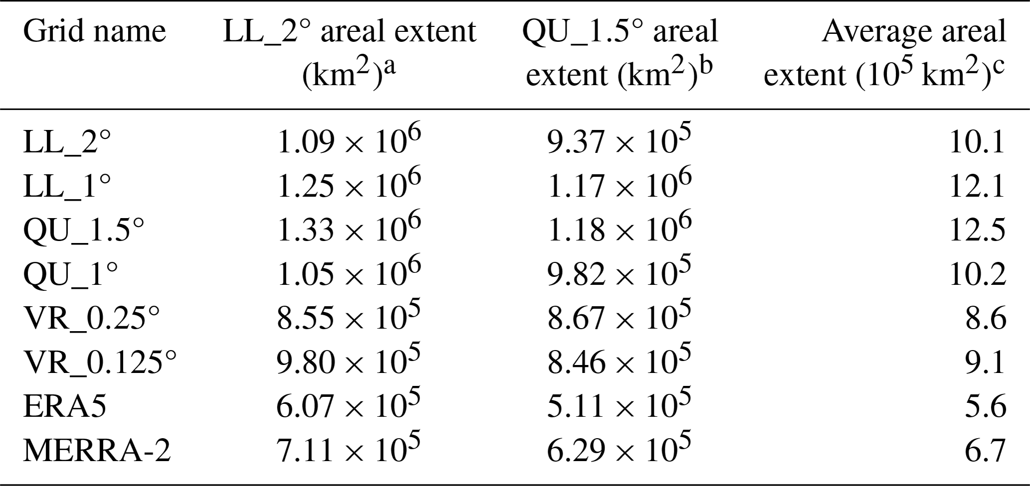
Herrington et al. (2022) ran CESM2.2 simulations using six different grid resolutions (Table 1, Fig. 1) from 1 January 1979 to 31 December 1998. These include a 2° latitude–longitude (LL) grid, LL_2° (Fig. 1a); a 1° LL grid, LL_1° (Fig. 1b); a 1° quasi-uniform unstructured (QU) grid, QU_1.0° (Fig. 1c); and another 1° QU grid but with the physical parameterizations evaluated on a coarser 1.5° grid (Herrington et al., 2019). We refer to this grid as QU_1.5° (Fig. 1d), but note the dynamics are still evaluated on the 1° grid. Finally, we use two variable-resolution (VR) grids, VR_0.25° (Fig. 1e) and VR_0.125° (Fig. 1f), with global spacing of 1° and increased spacing of 0.25 and 0.125°, respectively, around Greenland.

Table 1 Description of grid configurations.

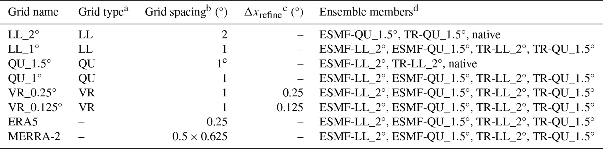
^a LL, latitude–longitude; QU, quasi-uniform; VR, variable resolution. ^b Average equatorial grid spacing. ^c Grid refinement for variable-resolution grids. ^d Remapped configurations performed that were included in the final ensemble. ESMF-LL_2°/TR-LL_2° and ESMF-QU_1.5°/TR-QU_1.5° refer to ESMF/TempestRemap methods which transformed native grids to LL_2° and QU_1.5°, respectively. Note that LL_2° and QU_1.5° grids were not remapped to themselves; their native grid configurations were used. ^e While QU_1.5° has the same 1° spacing as QU_1°, QU_1.5° has reduced-physics resolution, therefore degrading this 1° resolution.

Earth's topography is a boundary condition for CAM6 and is based on a 1 km resolution dataset (Danielson and Gesch, 2011). Software for processing this topography into CAM6 boundary conditions is described in Lauritzen et al. (2015). Figure 2 shows the impact of grid configuration on the resolution of the topography in Greenland. In the coarser grid configurations, LL (Fig. 1a–b) and QU (Fig. 1c–d), the elevation gradient from the coastal regions to the summit is not well represented. Additionally, high elevations in the center of the GrIS are smoothed in the coarser grids, resulting in a flatter ice sheet. In comparison, the high-resolution VR configurations (Fig. 1e–f) resolve gradients that are more similar to the reanalyses.

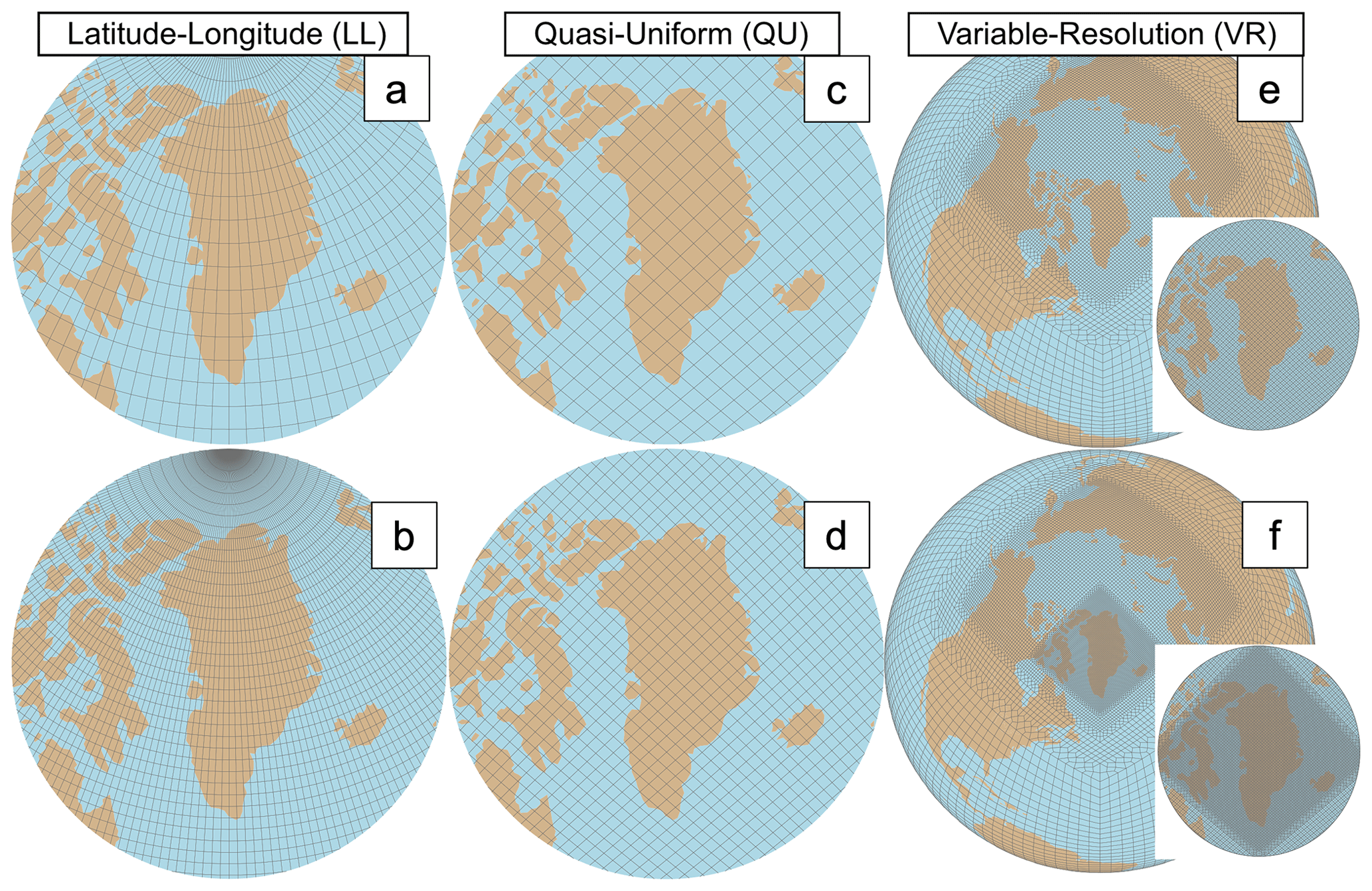
Figure 1 Grids used in this study. (a–b) Latitude–longitude (LL) (a – LL_2°, b – LL_1°) grids with higher resolution in polar regions. (c–d) Quasi-uniform (QU) (c – QU_1.5°, d – QU_1°) grids with more consistent resolution across the globe. (e–f) Variable-resolution (VR) (e – VR_0.25°, f – VR_0.125°) grids with insets emphasizing the higher resolution in the Arctic and Greenland. Lower-resolution grids are shown on the top row and high-resolution ones on the bottom row. Adapted from Herrington et al. (2022).

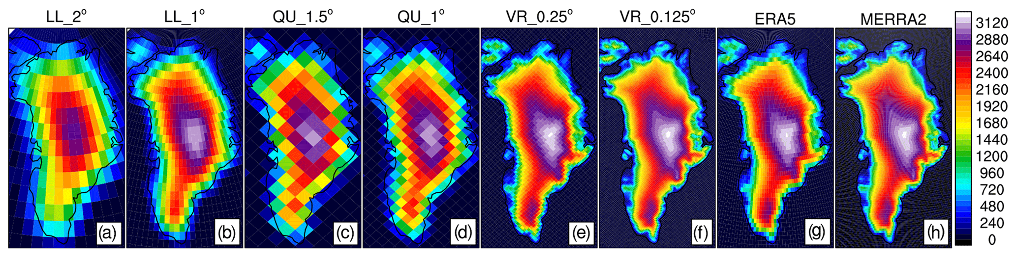
Figure 2 Native topography of each CESM2.2 grid configuration and reanalysis dataset used in this study. (a, b) Latitude–longitude (LL) (a – LL_2°, b – LL_1°) grids, (c, d) quasi-uniform (QU) (c – QU_1.5°, d – QU_1°), (e, f) variable-resolution (VR) (e – VR_0.25°, f – VR_0.125°) grids, (g) ERA5, and (h) MERRA-2.

2.2 Remapping

To control for the sensitivity of the algorithm of atmospheric feature detection to grid structure and resolution, we remapped the output from each simulation to the coarsest LL grid (LL_2°) and the coarsest QU grid (QU_1.5°) using two remapping methods, thus resulting in four ensemble members plus the two original coarsest grids (LL_2° and QU_1.5°) for a total of six grid configurations. This was a cautious choice as mapping to higher-resolution grids is inaccurate for first-order methods. The two remapping methods were ESMF (Balaji et al., 2021) and TempestRemap (Ullrich and Taylor, 2015), both of which use conservative formulations. For each simulation, the algorithm to identify and track ARs described in Sect. 2.3 was run six times, once for each of the four remapped ensemble members and the two coarsest (LL_2° and QU_1.5°) grids.

2.3 Detecting atmospheric rivers

Synoptic storms were tracked using TempestExtremes v2.1 software for atmospheric feature detection (Ullrich et al., 2021). This algorithm was chosen to detect ARs due to its usage of the Laplacian of the IVT rather than the IVT alone. The IVT is defined by

$$\begin{array}{}\text{(1)}& \mathrm{IVT}=\sqrt{{\mathrm{uIVT}}^{\mathrm{2}}+{\mathrm{vIVT}}^{\mathrm{2}}},\end{array}$$

where uIVT and vIVT are pointwise vertically integrated zonal and meridional vapor transport, respectively.

The gradients identified by the Laplacian method can detect ARs more accurately because there will still be a steep gradient between the AR itself and any surrounding moist area, thus better constraining the geometry of the AR (McClenny et al., 2020). Additionally, the use of IVT gradients rather than IVT values themselves generalizes the detection algorithm for use in climates with different amounts of atmospheric water vapor.

While this Laplacian threshold detects AR geometry well, it also allows non-AR features at high latitudes with similar geometries to be classified as ARs (see Sect. 3.1). Previous studies have noted the challenges of detecting polar atmospheric rivers due to the eastward–westward wind patterns that emerge (Rutz et al., 2019). There are many AR tracking algorithms that exhibit different behaviors and are suited to tracking ARs in specific locations (Shields et al., 2018). For example, when detecting Antarctic ARs, trackers that emphasize zonal IVT produce more accurate ARs than other algorithms (Shields et al., 2022). As our study focuses on the impact of resolution on ARs, including a limited number of high-latitude regions of moisture transport in the AR analysis does not affect the results.

Two algorithms from the TempestExtremes v2.1 package were used to detect and track ARs: one for detecting ARs (DetectBlobs) and one for stitching ARs together through multiple time steps (StitchBlobs). The detection algorithm searches the global extent for ARs that meet the following parameters: Laplacian of the IVT < −30 000 kg m⁻² s⁻¹ rad⁻², > 20° latitude, and areal extent ≥ 566 666 km². The Laplacian IVT threshold was chosen based on Rhoades et al. (2020a), Patricola et al. (2020), and Ullrich et al. (2021). Rhoades et al. (2020a) and Patricola et al. (2020) chose an IVT of −50 000 kg m⁻² s⁻¹ rad⁻², and Ullrich et al. (2021) used −20 000 kg m⁻² s⁻¹ rad⁻². The stricter threshold (−50 000 kg m⁻² s⁻¹ rad⁻²) resulted in too few ARs that made landfall in Greenland, but we still wanted to exclude smaller ARs that may not be of consequence in the GrIS. Thus, our threshold is in the middle of those used by others. The areal extent was chosen conservatively as two-thirds of the area of an average AR, which is 850 000 km² (Alan Rhoades, personal communication, 2022).

The output of the detection algorithm is a binary mask outlining candidate ARs, and the stitching algorithm is used to connect the blobs in time, providing each AR with its own unique identification number. The stitching algorithm links the ARs detected at each time step by the detection algorithm, rejecting candidate blobs that are not continuous in time. Using these two algorithms together, we track a single AR across its entire lifespan, from its origin in the mid-latitude regions through poleward transport to eventual dissipation. We chose to run the stitching algorithm using standard default settings based on optimizations from Alan Rhoades (personal communication, 2022). The number of ARs varied based on whether the native grid was remapped to LL_2° or QU_1.5° and the remapping method (Table 2). In addition to this AR tracking, we inventoried the origin points for each detected AR using the maximum IVT for that AR when first detected.

Table 2 The number of ARs overlapping the GrIS.

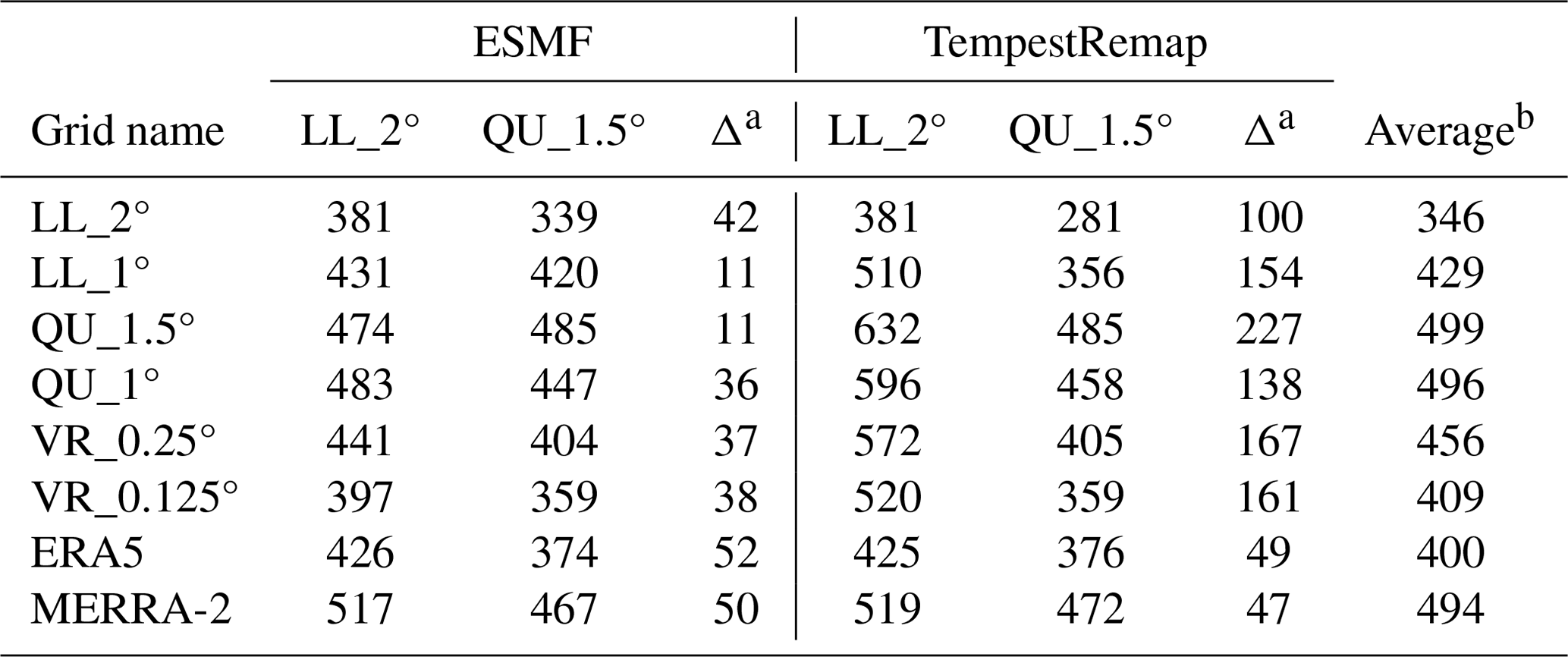
^a Difference (Δ) between LL_2°-detected and QU_1.5°-detected ARs overlapping the GrIS for each remapping method. ^b The average takes into account ESMF-LL_2°, ESMF-QU_1.5°, TempestRemap-LL_2°, and TempestRemap-QU_1.5°.

2.4 Compositing variables

To analyze the effects of ARs on precipitation over the GrIS, we first identified all ARs that overlap the GrIS at some point in their lifetimes. We counted all ARs touching the glacier land units of Greenland in CLM5, determined the overlapping area of these ARs at each time step, and calculated integrated precipitation from CAM6 output within these areas.

For each ensemble member, the tracker produces a binary mask array, $B_n^i\left(t\right)$, which contains 1s for times t and grid columns n where blob number i is active and 0s elsewhere. Note that there is only one horizontal dimension n, which is the convention for unstructured grids; a second horizontal dimension needs to be added when applying these equations to LL grids, e.g., $B_{x,y}^i\left(t\right)$.

We seek to find the time of maximum overlap for each blob, $t_c^i$, which we define as the time index in which the blob is maximally overlapping the GrIS. The area of the GrIS covered by blob i for time t is

$$\begin{array}{}\text{(2)}& a^i\left(t\right)={\sum }_{n=\mathrm{1}}^{\mathrm{ncol}}\mathrm{\Delta }{a}_n^i\left(t\right),\end{array}$$

where $\mathrm{\Delta }{a}_n^i\left(t\right)$ is the overlap area between the GrIS and blob i for each grid cell n,

$$\begin{array}{}\text{(3)}& \mathrm{\Delta }{a}_n^i\left(t\right)=f_n\mathrm{\Delta }{A}_n{B}_n^i\left(t\right).\end{array}$$

Here ΔA_n is area of each grid cell and f_n is the fraction of each grid cell covered by the GrIS. The time of maximum overlap $t_c^i$ is the time index t for each blob i where aⁱ(t) is a maximum. Of course, not all blobs descend upon the GrIS throughout their lifetimes. We therefore redefine i to denote the subset of blobs that overlap the GrIS at some point during their lifetime.

The integration of any arbitrary horizontal variable (e.g., precipitation), x_n(t), over the entire GrIS overlap area, coinciding with blob i in the vicinity of the time of maximum overlap $t_c^i+\mathit{\delta }t$, is performed as

$$\begin{array}{}\text{(4)}& X^i(t_c^i+\mathit{\delta }t)=\sum _{n=\mathrm{1}}^{\mathrm{ncol}}{x}_n(t_c^i+\mathit{\delta }t)\mathrm{\Delta }{a}_n^i(t_c^i+\mathit{\delta }t),\end{array}$$

whereas the area-average value of the variable x_n for blob i is

$$\begin{array}{}\text{(5)}& {\stackrel{\mathrm{‾}}{X}}^i(t_c^i+\mathit{\delta }t)={\displaystyle \frac{{\sum }_{n=\mathrm{1}}^{\mathrm{ncol}}{x}_n(t_c^i+\mathit{\delta }t)\mathrm{\Delta }{a}_n^i(t_c^i+\mathit{\delta }t)}{{\sum }_{n=\mathrm{1}}^{\mathrm{ncol}}\mathrm{\Delta }{a}_n^i(t_c^i+\mathit{\delta }t)}}.\end{array}$$

The time of maximum overlap $t_c^i$ is used to provide a common reference time for averaging the integrated quantities Xⁱ over all blobs.

We ran this AR characterization process over each of the four ensemble members (ESMF-LL_2°, ESMF-QU_1.5°, TempestRemap-LL_2°, TempestRemap-QU_1.5°) and took the average of each variable over the entire ensemble.

2.5 Validation

Reanalysis data from ERA5 and MERRA-2 were used to validate the ensemble-generated AR variables. The same remapping and compositing workflow that was applied to CESM2.2 simulations was applied to reanalyses. Meteorological reanalysis datasets combine observational data with a numerical atmosphere model to interpolate spatially and temporally onto a global grid. ERA5 is the fifth reanalysis dataset produced by the European Centre for Medium-Range Weather Forecasts (Hersbach et al., 2020). ERA5 data have a horizontal spatial resolution of roughly 27 km, and the variables chosen for this study have an hourly resolution, though we reprocessed this to a 6-hourly resolution to match the time steps in the CESM2.2 model outputs.

MERRA-2 uses available satellite data, observational data, and the Goddard Earth Observing System (GEOS) model to provide users with a spatially and temporally complete dataset (Gelaro et al., 2017). MERRA-2 has a horizontal resolution of 56 km (latitude) × 69 km (longitude) and 3-hourly temporal spacing, which we also reprocessed to a 6-hourly resolution.

These two reanalysis datasets were chosen for validation due to their frequent application in prior studies (Bresson et al., 2022; Marquardt Collow et al., 2022; Viceto et al., 2022; Zhou et al., 2022; Mattingly et al., 2023). The CESM2.2 model data and ERA5 share an overlapping study period of 1979–1998. Given that the available MERRA-2 data begin in 1980, we chose to include data available from 1980–1999 in order to maintain the same number of years in our study period (1979–1998).

It is important to emphasize that CESM2.2 simulations are free-running, coupled land–atmosphere climate simulations constrained by monthly sea-surface temperature and sea-ice extent but not by meteorological observations or reanalysis. We therefore present climatological comparisons among model configurations rather than historical observation-based case studies.

3 Results

3.1 Frequency, seasonality, and origin locations of atmospheric rivers

Between 7500 and 10 100 ARs were detected in the Northern Hemisphere across the six model configurations and the two reanalysis products between the years 1979–1998 (1980–1999 for MERRA-2) (Fig. 3). As MERRA-2 includes a different year (1999) than the modeled outputs and ERA5, we ensured that this year experienced a number of ARs that did not vary greatly from 1979–1998 before including it in our analysis. MERRA-2 resolved the highest number of ARs at 10 094, and the LL_2° detected the lowest number at 7514. We used the number of ARs overlapping the GrIS (Table 2) and ARs detected globally to calculate the percentage of ARs overlapping the ice sheet. This metric only varied from 4.0 % to 5.4 %, with ERA5 showing the lowest percentage of ARs reaching the GrIS.

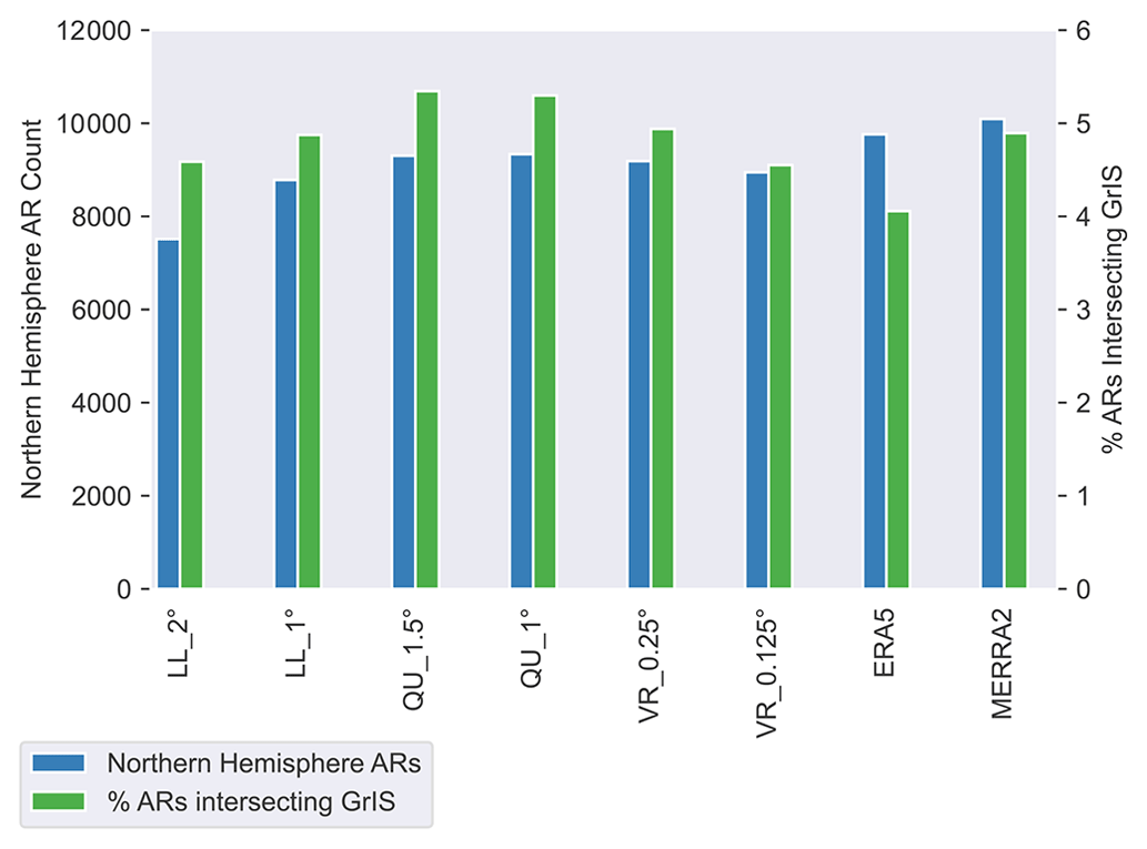
Figure 3 Average number of ARs in the Northern Hemisphere among the ensemble (left axis, blue). The average percentage of ARs overlapping the GrIS among the ensemble (right axis, green) normalized by total ARs, calculated using data available in Table 2.

The seasonal distribution of ARs reaching Greenland indicates that winter and spring generally have fewer ARs than summer and fall (Fig. 4). One or both VR grids produce the same median values as the reanalyses in every season. The QU grids produce the largest number of outliers of the grid configurations. When summed across the seasons, the number of ARs overlapping the Greenland ice sheet on an annual basis ranged from 10–37 per year depending on the grid configuration and specific year. There are large variations from year to year among the grid configurations, as is expected. The reanalyses produce annual variations that are similar to the spread of modeled simulations, therefore suggesting that the models produce ARs within or close to the bounds of reanalysis products.

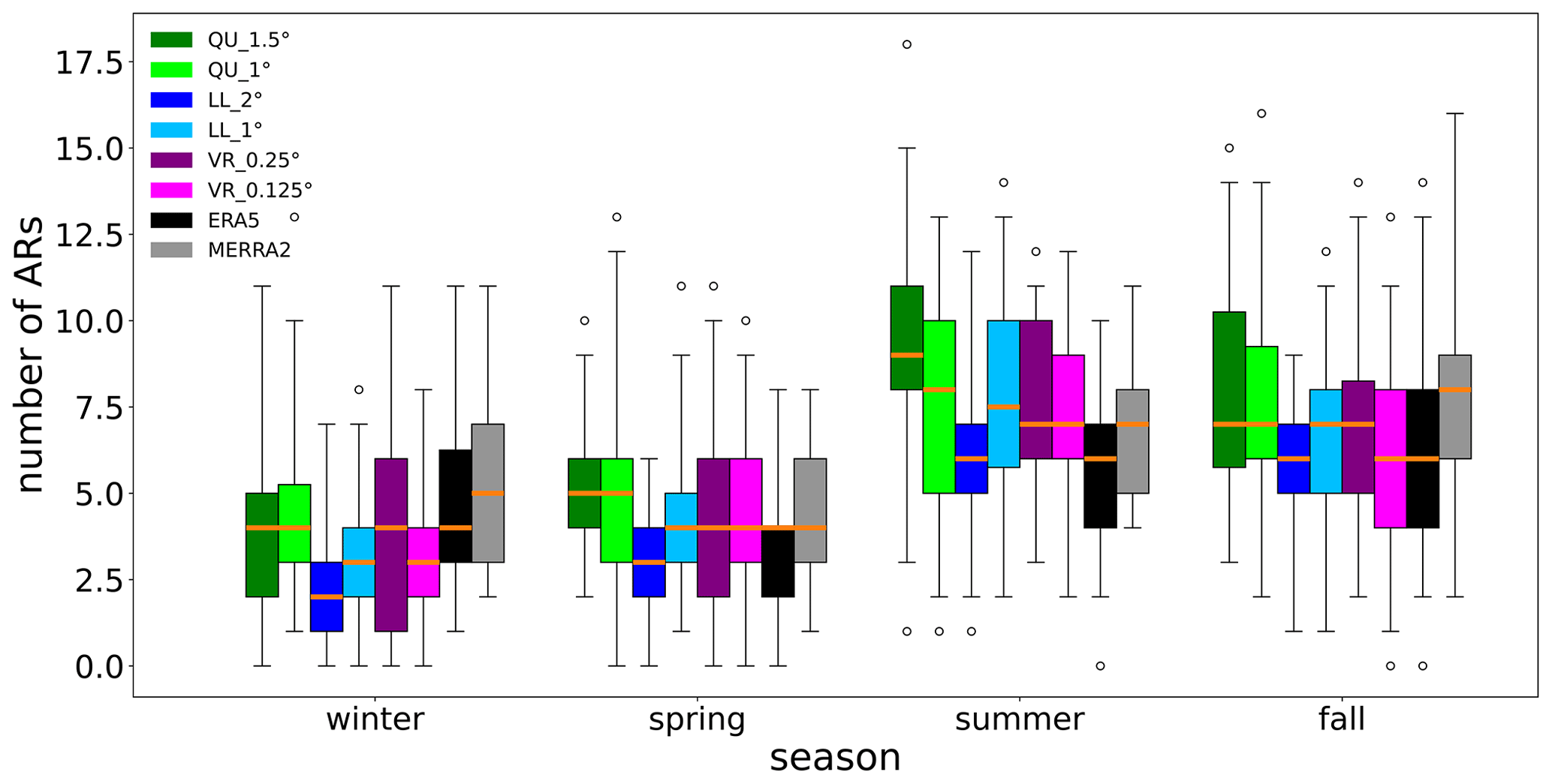
Figure 4 The number of ARs overlapping the Greenland ice sheet by season. Winter was defined as December through February, spring as March through May, summer as June through August, and fall as September through November. Seasonal distributions include 20 years of data (1979–1998) using values from each of the four remapped ensemble members (N=80). The orange line in the center of each box signifies the median value, and box lower and upper boundaries describe the 25 % and 75 % quartiles, respectively. The whiskers extend from the box to the 1st and 99th percentiles. Outliers outside these percentiles are indicated as open circles.

Figure 5 shows the origin locations for each AR that eventually overlaps the GrIS during summer months. The origin locations are determined by searching for the grid cell with the maximum IVT inside the AR at the first time that the AR is detected. Note that the location at which an AR forms is sensitive to the Laplacian of the IVT threshold used to identify ARs; a lower threshold means weaker IVT gradients and therefore designates AR origin points at lower latitudes earlier in the lifespan of an AR. Most ARs overlapping the GrIS during these months formed over the central United States from around 30–45° latitude. The next most frequent location for AR formation is over the western Atlantic at similar latitudes. While ARs are defined as originating in low to middle latitudes and transporting water vapor poleward, the detection algorithm identifies a small number of air masses with IVT characteristics above our detection threshold that originate at high latitudes. If these persist between time steps, the combination of the detection algorithm and the stitching algorithm categorizes them as ARs and they are retained in our analysis. Despite these outliers occurring at high latitudes, the majority of identified source regions are consistent with atmospheric rivers developing along mid-latitude storm tracks in relation to the baroclinic instability of extratropical cyclones. The reanalyses have more ARs that originate in the equatorial Atlantic compared to the model simulations.

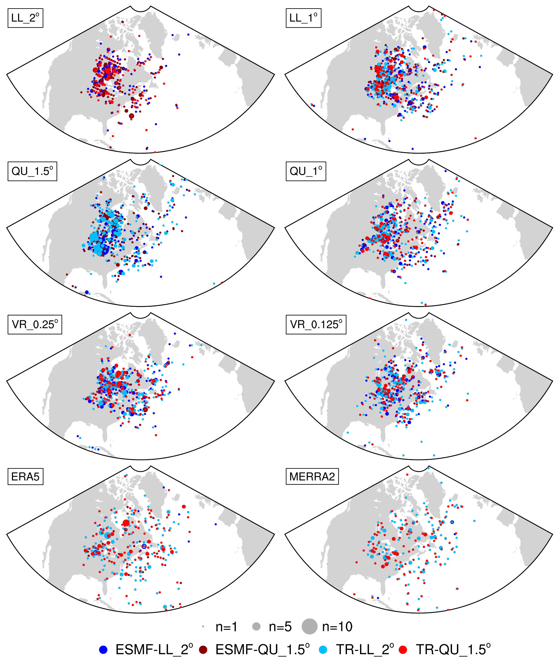
Figure 5 Origin of summer ARs that overlap the GrIS in JJA. The size and color of the dots indicate the number of ARs originating at a given location and the ensemble member represented, respectively.

3.2 Areal extent of atmospheric rivers

The areal extent describes the union of regions on the GrIS that overlap an AR for a particular grid configuration in this study. The VR simulations have the smallest footprints and are most similar to the reanalyses (Table 3). In nearly all cases, remapping to the QU_1.5° grid yields smaller footprints than remapping to LL_2°.

Table 3 Area of ARs overlapping the GrIS.

^a Values are the average of each of the LL_2° ensemble members (ESMF-LL_2°, TempestRemap-LL_2°). ^b Values are the average of each of the QU_1.5° ensemble members (ESMF-QU_1.5°, TempestRemap-QU_1.5°). ^c Values are the average of each of the four ensemble members (ESMF-LL_2°, ESMF-QU_1.5°, TempestRemap-LL_2°, TempestRemap-QU_1.5°).

The variation in footprint size is mainly due to the spatial distribution of ARs across the GrIS (Fig. 6). ARs most frequently make landfall with the southwestern and southeastern margins of the GrIS, and the number of ARs per grid cell rapidly declines moving inland for all configurations. ARs modeled with LL and QU grid configurations travel further inland than in the VR grids and reanalyses. It should also be noted that fewer ARs make landfall in the northern portions of the GrIS in ERA5 than in any of the other configurations. This lack of northern ARs (Fig. 6) explains why ERA5 has the lowest areal extent in Table 3.

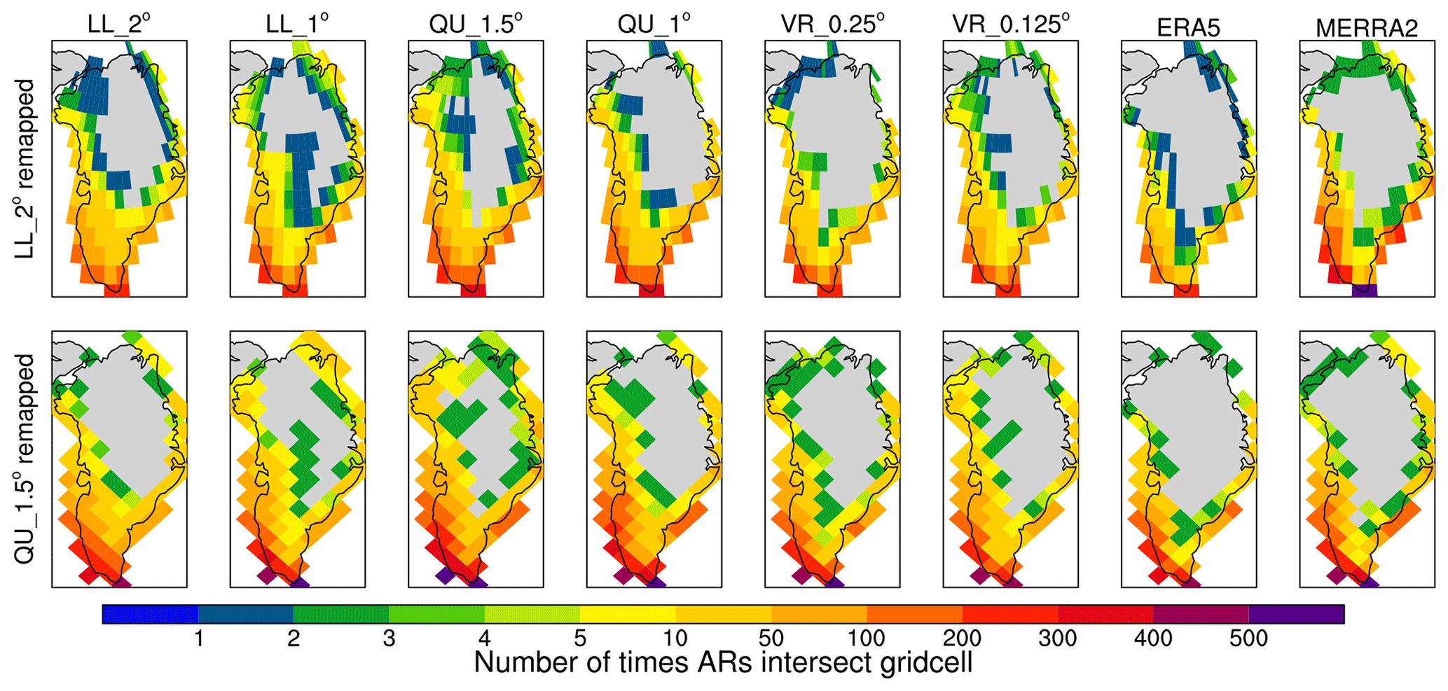
Figure 6 Spatial distribution of ARs over the GrIS using grid configurations remapped to LL_2° and QU_1.5°.

3.3 Number and size of atmospheric rivers

Figure 7a shows the number of ARs that eventually overlap the GrIS relative to the time of maximum overlap. Roughly 20 %–25 % of the ARs that make landfall have already formed 5 d before the time of maximum overlap (Fig. A1). This number of ARs increases until the time of maximum overlap, with the largest increase from 5 d to 2 d before the time of maximum overlap. This increase up to 1 d before the time of maximum overlap is likely due to ARs forming at high latitudes (Fig. 5). After the time of maximum overlap (i.e., Day 0; Fig. 7a), the number of ARs decreases for all grid configurations and reanalyses. The number of ARs 1 d after the time of maximum overlap is 25 %–50 % lower than the number of ARs during the time of maximum overlap. This means that many ARs rapidly dissipate, suggesting a large moisture transfer from the ARs to the GrIS, although some ARs do continue evolving until around 5 d past the time of maximum overlap.

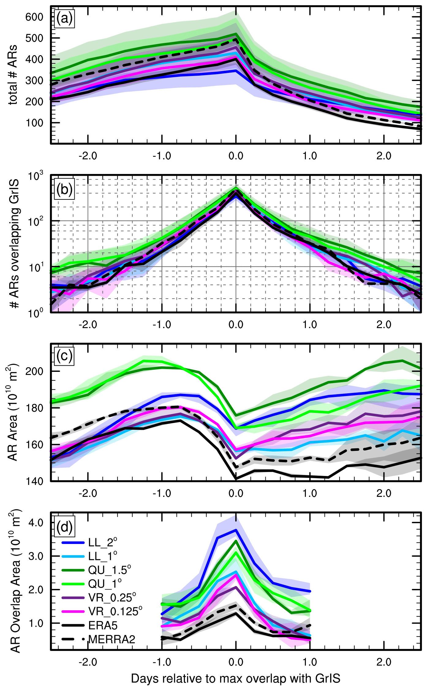
Figure 7 (a) The number of ARs that eventually overlap the GrIS as a function of time, normalized as days relative to the time of maximum overlap with the GrIS, and (b) the number of ARs overlapping the GrIS. (c) The area (m²) of ARs that eventually overlaps the GrIS and (d) the area (m²) of ARs that overlaps the GrIS.

Figure 7b describes the number of ARs overlapping the GrIS relative to the time of maximum overlap. The peak storm count at the time of maximum overlap in Fig. 7b is equal to the ensemble average of storm counts in Table 2. The QU grids produce more ARs than the rest, with LL, VR, and MERRA-2 in the middle and ERA5 producing the least. Figure 7b also shows that the majority of ARs pass over Greenland in 2 d, which is supported by previous research (Mattingly et al., 2020; Box et al., 2023). However, it seems that outside of the ± 1 d window from maximum overlap, the agreement between outputs degrades. Additionally, outside of that 1 d window, few ARs actually overlap the GrIS (< 10 ARs). Thus, needing a larger sample size to calculate meaningful statistics later on, we chose to analyze the ARs over the course of 2 d, centered by the time of maximum overlap.

There is a consistent and smooth increase in AR size for all grid configurations and the reanalyses 2 d before maximum overlap (Fig. 7c). This increase continues until 1 d before maximum overlap, when all configurations produce a sharp decrease in AR size due to a rapid reduction in moisture and/or winds. The QU configurations produce the largest ARs for almost the entire study period. After the time of maximum overlap, all of the simulations and reanalyses indicate changes in IVT that result in the AR area increasing in size again.

The area of an AR overlapping the GrIS also varies during its lifespan (Fig. 7d). In general, only a very small portion of each AR overlaps the GrIS. Average AR areas range from 140–200 × 10¹⁰ m² but less than 5.0 × 10¹⁰ m² of any AR overlaps the GrIS even during its time of maximum overlap. The LL_2° simulations have the largest overlap area during the time of maximum overlap and onward despite not having the largest AR area (Fig. 7c). Though the QU grids produce the largest ARs (Fig. 7c), they do not have the largest area of overlap with the GrIS. Reanalyses and the VR grids consistently produce smaller overlap areas.

3.4 Precipitation

When we plot the annual mean precipitation rate for all model grids and reanalyses on their native grids (Fig. 8), the lower-resolution grids tend to produce higher precipitation in the interior of the ice sheet, most notably over the southern dome of the GrIS. While the climatological mean precipitation rate is not exclusively from ARs, it exhibits a similar resolution sensitivity to our AR composite precipitation (Fig. 7).

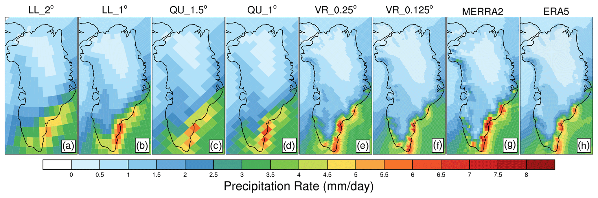
Figure 8 Annual mean precipitation rates (mm d⁻¹) for grids and reanalyses used in this study, plotted on their native grids.

ARs affecting Greenland make landfall on the coasts and travel inland. At this point, much of the moisture is deposited as precipitation and the storm dissipates. Figure 9 shows the composite precipitation map of all ARs as they travel over their storm path for one particular grid configuration and remapping scenario. The precipitation rates are largest at the time of maximum overlap with the GrIS, when the storms are at their most inland extent.

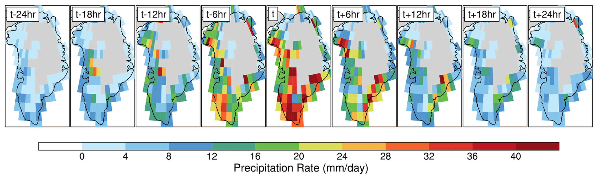
Figure 9 Average precipitation rates (mm d⁻¹) over the GrIS during ARs that make landfall in an example from VR_0.125° remapped to LL_2° using ESMF (n=520 ARs). Time t indicates the time of maximum overlap for the AR over the GrIS.

We used a 2 d window centered on the day of maximum AR overlap (Fig. 10a) to composite the area-average cumulative AR precipitation (hereafter, precipitation rate), using Eq. (5). At the end of the 2 d window, there is a difference of around 30 mm between the highest and lowest precipitation rates from the grid configurations and reanalyses. The configuration LL_1° produces the highest rate of precipitation, while MERRA-2 and LL_2° produce the lowest. ERA5 also produces magnitudes and trends of precipitation that are similar to the six modeled outputs.

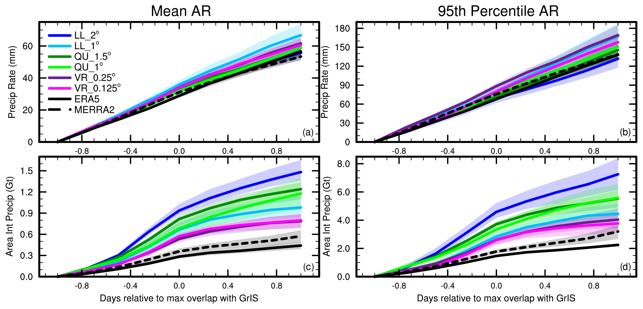
Figure 10 Cumulative precipitation metrics centered around the time of maximum AR overlap with the GrIS, including the (a) mean area-average precipitation rate, (b) 95th-percentile precipitation rate, (c) mean area-integrated cumulative precipitation, and (d) 95th-percentile cumulative precipitation over the GrIS. Time t indicates the time of maximum overlap for ARs over the GrIS. Precipitation is derived from 6-hourly average samples for ERA5 (PRECT), the 6-hourly average for MERRA-2 (PRECTOT), and 6-hourly instantaneous output for all model simulations (PRECC + PRECL).

Figure 10b compares the 95th-percentile AR precipitation rates. At the end of the study period, the 95th-percentile AR precipitation rates differ by about 40 mm, which is similar to the mean precipitation rates. Aside from the scales, the main difference between the mean and extreme rates is the ordering of the model grid configuration. VR_0.125°, VR_0.25°, and LL_1° produce higher precipitation rates than MERRA-2 and ERA5. This could be related to the model outputs being calculated using 6-hourly instantaneous output, whereas the observation-based data use 6-hourly averages.

Figure 10c compares the average area-integrated cumulative precipitation (hereafter, area-integrated precipitation) (Eq. 4), showing variation among model outputs and the two reanalyses. Area-integrated precipitation varies from around 0.7 Gt in ERA5 to 2.5 Gt in LL_2°. The two QU grids produce precipitation at the higher end of the spread, followed by LL_1°. The two VR grids simulate lower area-integrated precipitation than the other model grids. Both reanalyses produce less precipitation compared to the CESM2.2 model grids, though MERRA-2 produces similar precipitation magnitudes to VR_0.125°. There is a difference of about 0.1 Gt between VR_0.125° and MERRA-2 and about 0.4 Gt between VR_0.125° and ERA5. The trends in the rate of increase in the area-integrated precipitation are different than those seen in the precipitation rate (Fig. 10a); the highest rate of increase is during the day preceding the maximum overlap for all grid configurations except for LL_2°, after which it begins to slow.

Figure 10d compares the 95th-percentile area-integrated precipitation. VR_0.125° and VR_0.25° are the most similar model outputs to MERRA-2 and ERA5. In particular, VR_0.125° and MERRA-2 only differ by around 0.5 Gt in the extreme ARs.

A shortcoming of our approach is that we only composite the precipitation inside the tracked feature; however precipitation associated with an AR may include regions outside the tracked feature. Figures 11 and 12 show snapshots from the models and reanalyses, respectively, of the 95th-percentile ARs near the time of their maximum overlap with Greenland, and the outline of the detected feature is in magenta. The detected feature represents the moist core of the AR, which, unlike the larger synoptic system, does not overlap a large portion of land at any point throughout its life cycle (Fig. 7d). The snapshots indicate that the warm front out ahead of the AR core contributes a substantial amount of the storm's precipitation, which has been neglected from our precipitation composites thus far.

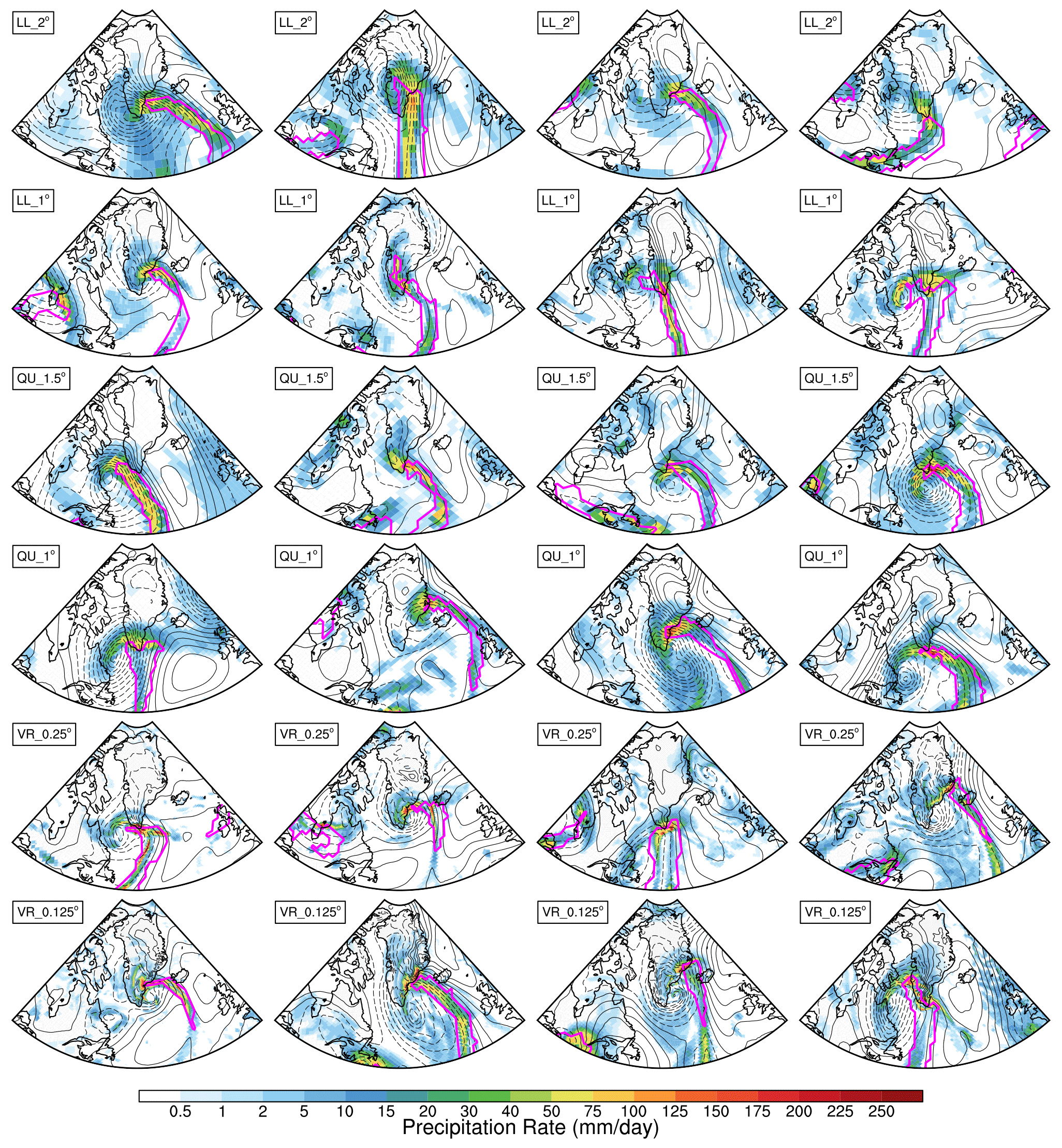
Figure 11 The 95th-percentile ARs and precipitation rates produced by LL, QU, and VR configurations on four different dates. ARs are outlined in magenta. Black contours are sea level pressure anomalies with 5 hPa intervals. Dates are not specified as model runs are freely evolving and do not reflect historical conditions.

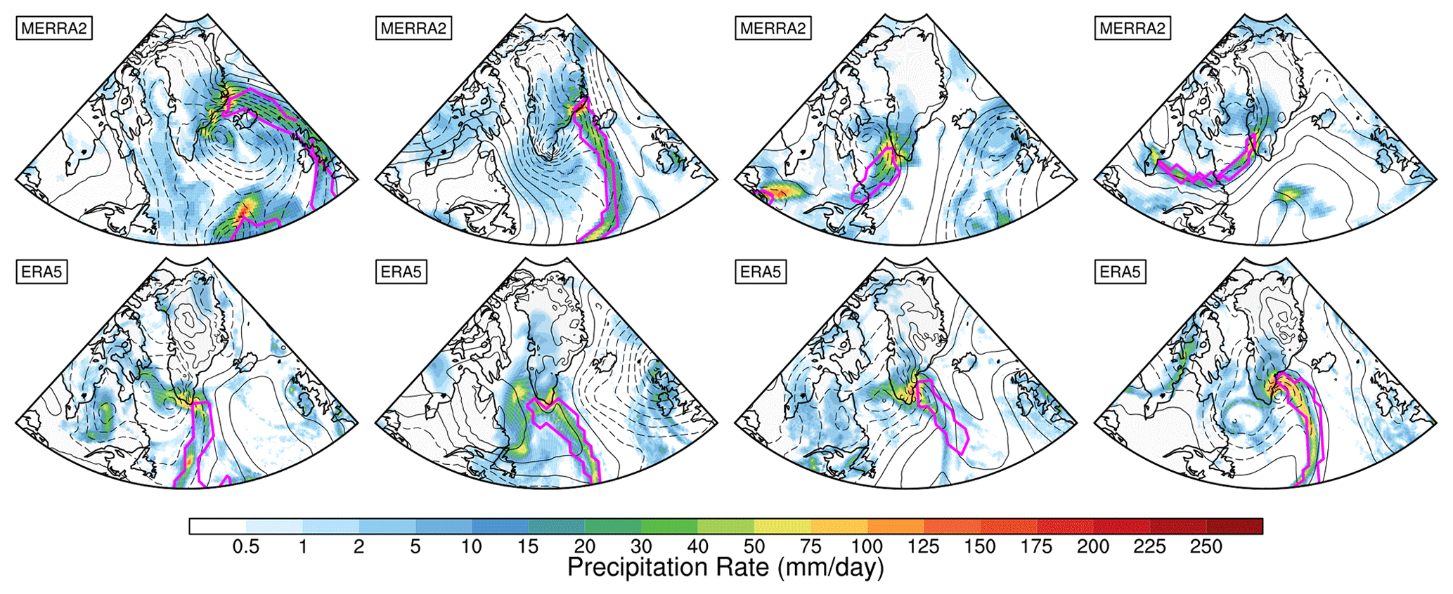
Figure 12 The 95th-percentile ARs and precipitation rates produced by MERRA-2 and ERA5 reanalyses on four different dates. ARs are outlined in magenta. Black contours are sea level pressure anomalies with 5 hPa intervals. Dates are not specified for the model AR example figure (Fig. 11) and therefore are also not given for this comparison reanalysis figure.

Figure 13a quantifies the impact of including regions outside the core of the AR on compositing precipitation due to that AR. It shows the precipitation rates over the 2 d window with respect to the radius of the expanded composite area. If a GrIS grid point lies within a radial great-circle distance to any point in the detected feature, it is included in the composite. From around 200 to 500 km, the precipitation rates steadily decrease, as regions are incorporated with smaller-magnitude precipitation rates in the composite. From 500 km onward, the precipitation rates decrease at a slower rate, suggesting a transition to the marginal outer regions of the synoptic system which may not be exclusively associated with the storm itself. All model outputs and reanalyses exhibit similar behavior, mainly differing in their maximum precipitation rates, with LL_1° having the largest and MERRA-2 the smallest.

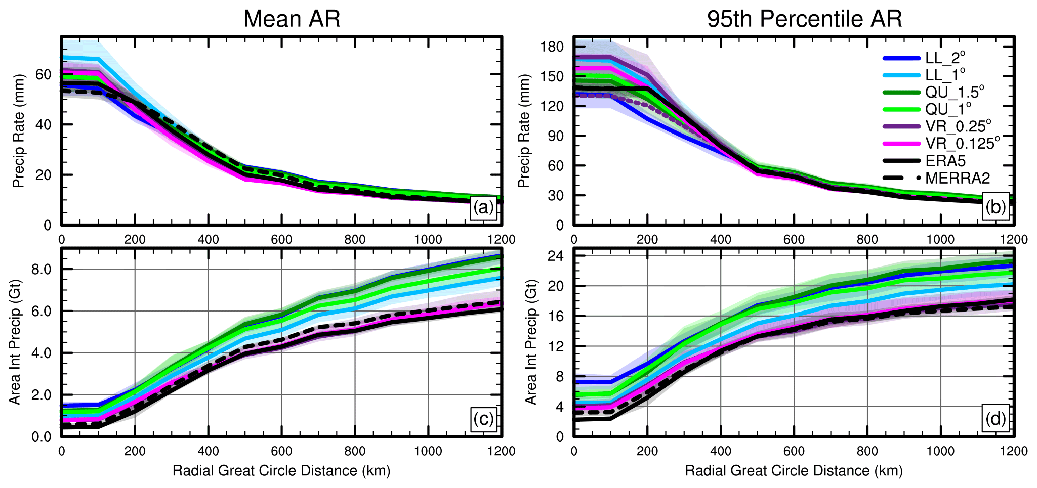
Figure 13 (a) Mean precipitation rates, (b) 95th-percentile precipitation rates, (c) mean area-integrated precipitation, and (d) 95th-percentile area-integrated precipitation over the GrIS compared to the radial great-circle distance of GrIS grid points to ARs. The radial great-circle distance (km) describes the distance of each grid point on the GrIS to an AR. Precipitation is derived from 6-hourly instantaneous output in the model runs, whereas the reanalyses use 6-hourly averaged precipitation. The dashed purple line in (b) is the VR_0.25° run but using two-point averaging to estimate the impact of using averaged variables in the reanalyses.

Figure 13c shows the 2 d area-integrated precipitation with respect to the radial great-circle distance. Similarly to the precipitation rates, the integrated precipitation does not change from 0 to 100 km, as we are analyzing model and reanalysis output mapped to the two coarsest-resolution grids. From 200 to 500 km, the area-integrated precipitation increases due to incorporating a larger area of the GrIS, which has, however, smaller precipitation rates (Fig. 13a). In combining Fig. 13a and c, we can estimate that most GrIS precipitation which is associated with an AR occurs within around 500 km of the tracked feature. At this 500 km mark, the reanalyses produce between 4.0 and 4.5 Gt of precipitation with both VR outputs well within these bounds. The LL and QU produce between 4.5 and 5.5 Gt, and the differences between VR and LL/QU are even larger at the 1200 km distance. While the coarser grids overestimate GrIS precipitation from ARs, LL_1.0° is by far the most skillful (Figs. 10c and d and 13c). This is due to the approximate 0.5° representation of the GrIS on the LL_1.0° grid (Herrington et al., 2022).

The 95th-percentile AR precipitation rate (Fig. 13b) and area-integrated precipitation (Fig. 13d) exhibit a similar dependence on the great-circle distance to the mean ARs, although with larger magnitudes. At a radial distance of 500 km, the reanalyses produce roughly 13 Gt of precipitation, which is extremely well captured with VR outputs. At 500 km, the LL and QU grids produce between 15–17 Gt of precipitation. However, unlike the mean ARs, there is no reduction in the precipitation rate from 0 to 200 km in both reanalysis products. As was suggested for the smaller-magnitude precipitation rates in the reanalysis (Fig. 10b), this might be due to differences in tracking features and compositing precipitation using 6-hourly average reanalysis output instead of 6-hourly instantaneous output.

The time averaging smooths the precipitation and IVT fields over a length scale determined by the storm's motion and overall evolution, as well as length of time. This averaging degrades the representation of individual features, which is consistent with only small variations in precipitation in the vicinity of the AR boundary in the reanalyses (Fig. 13b). We estimate the impact of time averaging on the VR_0.25° run (Fig. 13b). The dashed purple line shows the 95th-percentile precipitation rate after two-point-averaging the 6-hourly instantaneous output for tracking the AR and compositing precipitation in the VR_0.25° run. The averaging reduces the magnitude of the precipitation rate and also reduces the variation across the inner 200 km radial distance (Fig. 13b). The reanalysis precipitation rates at the scale of the detected features are smoothed by the time averaging and cannot serve as a reliable model target for area averages over the detected features (Eq. 5; Fig. 10). That is, we do not conclude that the VR precipitation rates are overestimated in Fig. 10 but rather suggest that the reanalysis precipitation rates and (related) area-integrated precipitation are underestimated.

The 6-hourly time averaging does not impact the precipitation rates when averaged over larger areas. The VR_0.25° precipitation rates are insensitive to two-point averaging when integrated out to the 500 km radial AR boundary (Fig. 13b). We conclude, based on Fig. 13c–d, that the VR grids are able to reproduce the reanalysis and are therefore skillful at simulating precipitation on the GrIS due to ARs.

4 Discussion

We hypothesize that the higher and steeper topography resolved in VR grids and the reanalyses prevents ARs from penetrating as far inland as the ARs do in the LL and QU grids. The finer-resolution VR grids and reanalyses produce smaller ARs (Fig. 7c), consistent with more precise tracking of atmospheric moisture. However, the large GrIS overlap of ARs in LL_2° (Fig. 7d) is not related to the size of ARs prior to landfall (Fig. 7c), supporting the hypothesis that topographic smoothing explains the variations in AR areal overlap with the GrIS.

Coarser grids require more topographic smoothing to prevent the excitation of inaccurate grid-scale modes in the dynamical core (Lauritzen et al., 2015). In the LL and QU grids, topographic smoothing is ubiquitous across the GrIS (Fig. 2) and allows moisture to penetrate further into the interior of the ice sheet, reducing orographic lifting that would otherwise drain ARs of their moisture and cause them to dissipate (Pollard, 2000; Box et al., 2023). For example, the LL_2° grid has the lowest maximum elevation for the GrIS and the largest AR areal extent. In contrast, the VR grids and reanalysis datasets all have similar topography, capturing high elevations and steep elevational gradients across the GrIS.

The differences in area-integrated precipitation among grid configurations (Figs. 10c–d, 13c–d) reflect the areal extents of ARs over the GrIS (Table 3, Fig. 7d). As the precipitation rates are similar across all grids, simulated ARs that cover a larger areal extent of the GrIS deposit more total precipitation. ERA5 produces the lowest area-integrated precipitation, followed by MERRA-2 and both VR grids, with the LL and QU grids producing the most precipitation. These findings are consistent with the sensitivity of the mean annual precipitation and mass balance across grid resolutions in prior VR CESM studies (Herrington et al., 2022; van Kampenhout et al., 2020).

Previous studies support our hypothesis. Huang et al. (2016) and Rhoades et al. (2020b) have shown that the ability of VR grids to better resolve ARs in regions of complex topography leads to improved simulated climate and snowpack in California. Ikeda et al. (2010, 2021) have found similar results describing the high resolution needed to resolve precipitation and flow around steep topography in the western United States. Regional modeling studies from Ettema et al. (2009) and Franco et al. (2012) have also found that reduced topographic smoothing for higher-resolution simulations improves storm precipitation in Greenland.

The origin locations and behavior of modeled ARs aligned with observations. We found that many ARs overlapping the GrIS initially form over the mid-latitude central United States (Fig. 5), consistent with Neff et al. (2014). Our tracking algorithm also identified a subset of ARs at uncharacteristically high latitudes, suggesting that a more polar-optimized tracking algorithm should be used around Greenland (Shields et al., 2023). Alternatively, these high-latitude ARs might challenge the typical definition of ARs – does an AR need to form at low to middle latitudes, or are there actually ARs forming at such high latitudes, as Komatsu et al. (2018) and Mattingly et al. (2023) suggest?

ERA5 and MERRA-2 differ in their geographic distribution of ARs over the GrIS, suggesting the need to consider multiple reanalyses when studying precipitation from ARs in Greenland. While VR grids and MERRA-2 produce many ARs making landfall in the northern regions of the GrIS, ERA5 shows very few. Recent studies investigating ARs impacting the northern GrIS support the finding that ARs do occur at such high latitudes in this region (Mattingly et al., 2023).

5 Conclusions

This study uses CESM2.2 simulations from Herrington et al. (2022) to compare six grids in modeling ARs and related precipitation over the GrIS. The 1–2° LL grid configurations provide enhanced resolution over polar regions with some reduction in resolution caused by a polar filter to prevent numerical instability. Two QU grids maintain roughly 1–1.5° uniform resolution across the globe. To study the impact of resolution on ARs around the GrIS, we compare simulations using these four coarser grids to two VR grids using a spectral-element dynamical core (dycore), VR_0.25° and VR_0.125°.

We developed a method that maps all output to the two coarsest model grids using two different remapping methods to account for uncertainty in comparing AR statistics in model simulations and reanalysis products across vastly different grids. We use the overlap area of an AR and the GrIS to determine how AR characteristics and precipitation vary based on grid configuration. This method identifies precipitation from regions of the GrIS that an AR is directly overlapping at a point in time and sums the precipitation in each of these regions by grid configuration. This allows for a robust comparison of precipitation across grids with realistic uncertainty. We also employ a method that expands on the area directly below an AR to better estimate precipitation derived from these events. Ideally this method can also be applied to other variables relevant to ARs and the GrIS, including snowmelt and radiative fluxes (Mattingly et al., 2020; Kirbus et al., 2023).

We find that the topographic resolution of the grid likely constrains AR penetration into the GrIS. In coarser-resolution grids, there is greater topographic smoothing of the GrIS and ARs can travel further inland. As precipitation rates do not vary greatly across grid configurations, the overlap extent of ARs largely determines the simulated precipitation falling onto the GrIS. Additionally, we see consistent patterns that characterize AR behavior and lifespan around the GrIS. In the CESM2.2 simulations and reanalyses, most ARs only overlap the GrIS for around 1 to 2 d. ARs increase in intensity prior to landfall, and immediately before the time of maximum overlap, ARs experience a “draining period” and decrease in size, likely due to orographic uplift that drains the ARs of their moisture. The role of smoothed topography could be further explored by running the model with the VR grid but using the same lower-resolution topography as the coarser grids.

Finally, we find that the VR grids produce AR areal extents, area-integrated precipitation, and AR sizes that are most similar to the reanalysis datasets ERA5 and MERRA-2. All CESM2.2 simulations produce higher values for all three AR metrics than the reanalyses. Although VR grids deviate somewhat from the reanalyses, VR grids outperform the LL and QU grids used in our study and have resolutions approaching regional climate models but at lower computational costs. We therefore recommend that modeling studies of ARs around Greenland consider using CESM2.2 VR grid configurations as an alternative to uniform grids.

Appendix A: The 10 d atmospheric river size and Greenland ice sheet intersection simulation

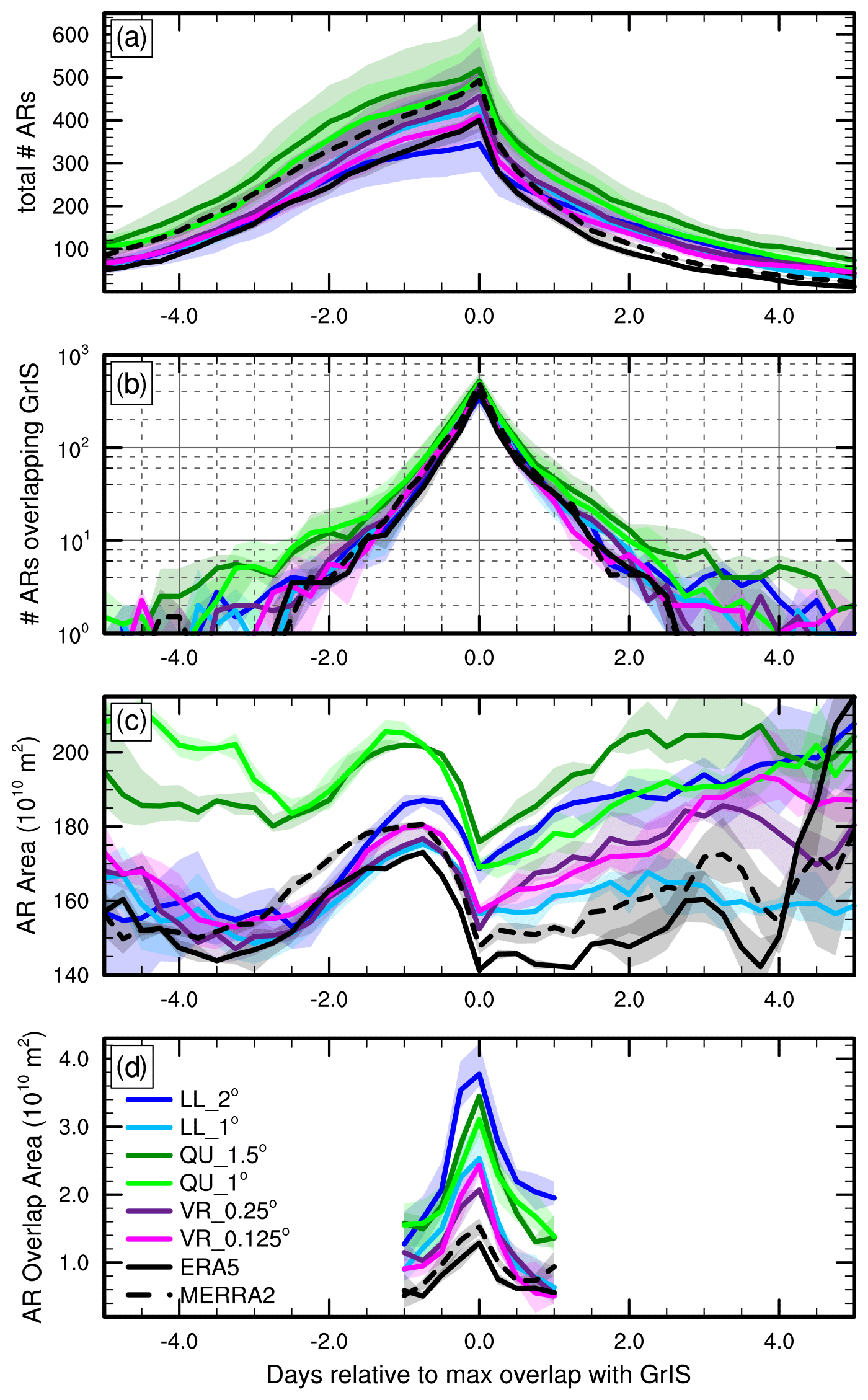
Figure A1 (a) The number of ARs that eventually overlap the GrIS as a function of time, normalized as days relative to the time of maximum overlap with the GrIS, and (b) the number of ARs overlapping the GrIS. (c) The area (m²) of ARs that eventually overlaps the GrIS and (d) the area (m²) of ARs that overlaps the GrIS, showing that only a small portion of each AR overlaps the GrIS. As data are noisy at the beginning and end of the 10 d period, the main text only includes ±2.5 d.