the Creative Commons Attribution 4.0 License.
the Creative Commons Attribution 4.0 License.
 | 14 Jun 2024
Large-scale perspective on extreme near-surface winds in the central North Atlantic
Aleksa Stanković
Gabriele Messori
Joaquim G. Pinto
Rodrigo Caballero
This study investigates the role of large-scale atmospheric processes in the development of cyclones causing extreme surface winds over the central North Atlantic basin (30 to 60° N, 10 to 50° W), focusing on the extended winter period (October–March) from 1950 until 2020 in the ERA5 reanalysis product. Extreme surface wind events are identified as footprints of spatio-temporally contiguous 10 m wind exceedances over the local 98th percentile. Cyclones that cause the top 1 % most intense wind footprints are identified. After excluding 16 (14 %) of cyclones that originated as tropical cyclones, further analysis is done on the remaining 99 extratropical cyclones (“top extremes”). These are compared to a set of cyclones yielding wind footprints with exceedances marginally above the 98th percentile (“moderate extremes”). Cyclones leading to top extremes are, from their time of cyclogenesis, characterised by the presence of pre-existing downstream cyclones, a strong polar jet, and positive upper-level potential vorticity anomalies to the north. All these features are absent or much weaker in the case of moderate extremes, implying that they play a key role in the explosive development of top extremes and in the generation of spatially extended wind footprints. There is also an indication of cyclonic Rossby wave breaking preceding the top extremes. Furthermore, analysis of the pressure tendency equation over the cyclones' evolution reveals that, although the leading contributions to surface pressure decrease vary from cyclone to cyclone, top extremes have on average a larger diabatic contribution than moderate extremes.
- Article
(5232 KB) - Full-text XML
- BibTeX
- EndNote


The weather and climate of Europe are strongly influenced by the passage of extratropical cyclones. Cyclones are the main cause of wind and precipitation extremes during the winter season over the Euro-Atlantic sector (Fink et al., 2009; Pfahl and Wernli, 2012) and routinely generate large wind-related economic losses across the continent (Roberts et al., 2014). This makes extreme cyclones and the associated windstorms one of the leading natural hazards in Europe (Berz, 2005; Ulbrich et al., 2013a; Spinoni et al., 2020).
Various aspects of extreme extratropical cyclones affecting Europe have been examined in previous work, including several detailed case studies of some of the most damaging historical windstorms, like Lothar, Kyrill, and Xynthia (Wernli et al., 2002; Fink et al., 2009; Rivière et al., 2010; Ludwig et al., 2014, 2015), and studies focusing on identification of common features, from large-scale to mesoscale (see for example Earl et al., 2017, who focused on UK wind gusts by analysing observational data), associated with extreme windstorms caused by cyclones. Hanley and Caballero (2012b) and Messori and Caballero (2015) analysed the most salient features of the large-scale atmospheric flow in which some of the most destructive European windstorms were embedded. They showed that surface wind extremes over Europe often coincide with simultaneous cyclonic and anticyclonic Rossby wave breaking events in the eastern part of the North Atlantic basin. Gómara et al. (2014) further demonstrated a positive correlation between Rossby wave breaking and the occurrence of explosive cyclones in the Euro-Atlantic sector. They found that the most intense cyclones in the western North Atlantic were associated with cyclonic Rossby wave breaking over western Greenland, while the most intense cyclones in the eastern North Atlantic were preceded by cyclonic Rossby wave breaking over eastern Greenland or anticyclonic Rossby wave breaking in the subtropical North Atlantic. The physical basis of these results lies in how wave breaking events influence the orientation and strength of the eddy-driven jet. Specifically, they can create favourable conditions for cyclone intensification by strengthening upper-level divergence in the right-entrance and left-exit regions of the jet core (Uccellini, 1990). Dacre and Pinto (2020) showed that interactions between Rossby wave breaking and the eddy-driven jet are also important for cyclone clustering, i.e. the passage of multiple cyclones over a fixed location within a given time period. Although the individual cyclones that pass in succession through the same region might not be extreme, the accumulated impact of wind damage and/or precipitation can be extreme when compared to individual events. Rossby wave breaking can further influence the strength and tilt of the jet, which can then steer multiple cyclones towards the same region (Pinto et al., 2014; Messori and Caballero, 2015; Priestley et al., 2017).
An approach complementary to those above takes the potential vorticity (PV) perspective (Hoskins et al., 1985). This framework evaluates cyclone evolution through the lens of interactions between positive PV anomalies at different levels and positive potential temperature anomalies at the surface, which all induce a cyclonic circulation. This perspective has been used to study individual historical storms (like Lothar in Wernli et al., 2002) and to develop climatologies of cyclones (Čampa and Wernli, 2012). By studying PV towers (i.e. positive PV anomalies vertically aligned from the tropopause to the surface) associated with extratropical cyclones in the Northern Hemisphere, Čampa and Wernli (2012) found that more intense cyclones (in terms of lower sea level pressure) are, on average, associated with more prominent lower- and upper-level PV anomalies. The PV framework was also applied to climate model simulations to study future changes in North Atlantic cyclones and near-surface winds associated with them (for example in Dolores-Tesillos et al., 2022).
The hazard to life and property posed by land-falling cyclones and associated extreme winds motivates the broad literature on the topic, part of which we have outlined above. However, land-falling cyclones constitute only a small fraction of the total number of cyclones that occur over the oceanic basins. In particular, since Europe is located at the end of the Atlantic storm track, cyclone track density there is lower compared to its peak in the central Atlantic (Wernli and Schwierz, 2006; Dacre and Gray, 2009). Notwithstanding extensive research on various aspects of North Atlantic cyclones, there have been few studies specifically focused on studying cyclones that cause extreme surface winds over the ocean (de León and Bettencourt, 2021, analysed wave heights from altimetry data, while Gentile and Gray, 2023, investigated winds in the part of the Atlantic Ocean surrounding the British Isles). However, investigation of windstorms over the ocean is of interest for several reasons. Focusing on extreme windstorms over the ocean provides the opportunity to study cyclones that cause extreme 10 m winds in the region of peak cyclone track frequency. An analysis of this kind is thus useful to compare mechanisms driving extreme windstorms over the bulk of the oceanic storm track and over Europe, which is at the end of the North Atlantic storm track. Moreover, the chosen target region provides a larger sample of intense windstorms than if focusing on land regions, which is an important aspect to consider when studying any extreme event. An additional reason for choosing an ocean region is that it removes the sometimes confounding effects of topography and land surface properties, enabling a more direct link between cyclone characteristics and surface wind footprints. On a more practical note, offshore infrastructure and busy shipping routes over the North Atlantic can be severely affected by extreme winds, resulting in sizeable insured losses (Cardone et al., 2015). Finally, strong winds drive intermittent deepening of the ocean mixed layer, affecting phytoplankton bloom dynamics in the North Atlantic (e.g. Lacour et al., 2017).
Here, we aim to address the above knowledge gap and specifically answer the following question: what are the large-scale atmospheric factors favouring the development of extreme surface winds in the North Atlantic basin? The highest median and 98th percentiles of 10 m wind speed in the Atlantic sector occur in the central basin, approximately in the region covering 10–50° W and 40–60° N during the winter (Laurila et al., 2021b). In this study we thus focus on this region. In contrast to many earlier studies that focused on explosive cyclones or cyclone clustering in this region, we apply a bottom-up approach, whereby we first identify extreme 10 m wind events and then study the cyclones associated with them. We investigate how these cyclones differ from weaker cyclones as regards the synoptic-scale features present during their development, their connection with the upper-level potential vorticity fields and their anomalies, and the strength of the eddy-driven jet with which they interact. Additionally, we perform a surface pressure tendency analysis to quantify the factors behind deepening of top-extreme and moderate-extreme cyclones. The data and methods used are described in Sects. 2 and 3, respectively. In Sect. 4 we present results based on a composite analysis of the extreme 10 m wind events, alongside a quantitative decomposition of the mechanisms driving the deepening of the associated cyclones. The results are discussed in Sect. 5, where we argue that the presence of a pre-existing downstream cyclones is of critical importance for development of the extreme-wind-causing cyclones. We summarise our conclusions in Sect. 6.
We use the ERA5 global atmospheric reanalysis from the European Centre for Medium-Range Weather Forecasts (Hersbach et al., 2020). We consider hourly data from 1950 to 2020 with 0.25° (∼ 31 km) horizontal resolution. We analyse 10 m and 250 hPa horizontal wind components, PV from 900 hPa up to 200 hPa (18 levels), and mean sea level pressure (MSLP). It should be noted that ERA5 has known biases when it comes to 10 m wind speed; in particular, ERA5 tends to have 8 %–10 % lower values of the most extreme (95th and 99th percentiles) 10 m winds over the North Atlantic Ocean compared to satellite observations (Campos et al., 2022). However, since biases are similar across the target region of our study (Campos et al., 2022), we do not expect these biases to affect the ranking of our events. Additionally, studies comparing extreme 10 m winds from ERA5 to observations over the continents suggest that the variability of extreme 10 m wind speeds across cyclone centres is still well reproduced even with underestimation of 10 m wind speeds, despite the much more complex topography (Chen et al., 2024). This gives further assurance that 10 m winds from ERA5 are a reliable tool to rank the most extreme wind events.
We focus only on cyclones originating in the extratropics, excluding tropical cyclones undergoing extratropical transitions (for an explanation of why extratropical transitions are excluded, see discussion in the next section). To this end, we use post-storm analyses (best track intensity and position estimates) of Atlantic tropical cyclones from the HURricane DATabase (HURDAT; Jarvinen et al., 1984). Although HURDAT goes back to 1851, the accuracy and completeness of the dataset increase after the introduction of aircraft reconnaissance (1944 for western part of the basin) and satellites (NOAA, 2023), so its use is appropriate for the 1950–2020 period studied here.
3.1 Extreme 10 m wind speed event selection
We focus on the extended winter season (October–March) from 1950 until 2020. Figure 1 shows the target region, spanning 10 to 50° W and 30 to 60° N. Extreme event detection is based on a meteorological wind severity index – for brevity referred to simply as severity throughout the paper – defined following previous work on European windstorms (Klawa and Ulbrich, 2003; Pinto et al., 2012; Hanley and Caballero, 2012b). A similarly defined index has also been applied to climate model outputs in previous work (Leckebusch et al., 2008).
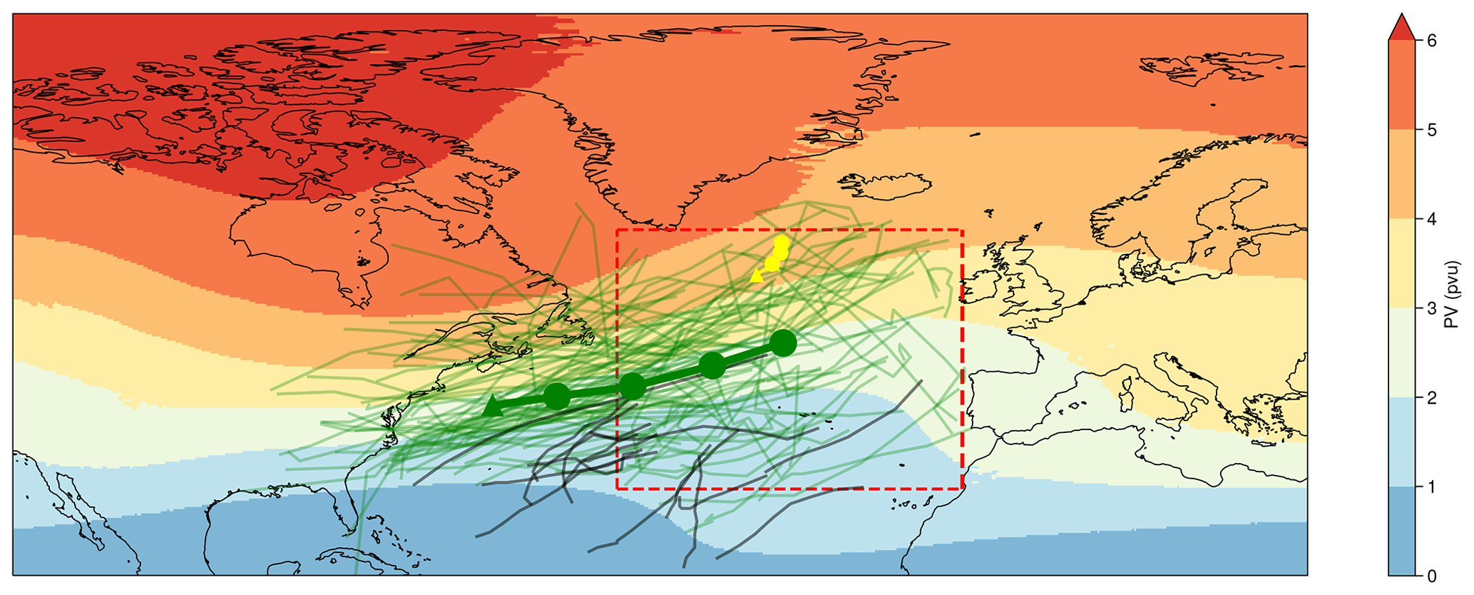
Figure 1Upper-level PV (200–300 hPa mean) climatology for extended winter season (Oct–Mar) from 1950 to 2020 (colours). The red box shows the target region used to study windstorms. Storm tracks of extratropical and top-extreme cyclones (green lines) and tropical cyclones (black lines) associated with the top 1 % 10 m wind severity events from 2 d before until the time of maximum 10 m wind speed. Average 12-hourly track of top extremes is shown as a thick green line, with the green triangle representing the mean location of cyclogenesis of top extremes. The average storm track of the pre-existing downstream cyclones from 2 d to 12 h before the peak 10 m winds is shown as a yellow line, with the yellow triangle showing their mean location at the time of cyclogenesis of top extremes.
Our severity index takes into consideration grid cells where the daily maximum 10 m wind speed exceeds its local 98th percentile. We calculate severity for any given day as follows. First, we find out if there are any connected regions within the target domain where daily maximum 10 m wind speed has exceeded the local 98th percentile. We call such regions wind footprints. If wind footprints exist, the severity index S for each one of them is calculated as
where i indexes all the grid cells within the connected wind footprint, vi is the daily maximum wind speed at grid point i, is the local 98th percentile with respect to the extended winter climatology from 1950 to 2020, and if a>b and 0 otherwise.
We calculate severity for every day in our dataset and select days on which severity is greater than 0. We then retain the top 1 % of these days for further analysis, which corresponds to 115 d. More than one wind footprint can exist for any given day over the study area. If that is the case, we take the largest severity value as the severity for that day. The reason for calculating separate values of severity for different wind footprints within the target region is that there can be multiple cyclones passing through the target region on the same day. Identifying contiguous regions reduces the possibility of attributing a footprint to the wrong cyclone. It should also be noted that if a given windstorm caused exceedances in connected regions outside of the target region, those regions are disregarded in order to focus on the target region. A simplified illustration of our analysis procedure is shown in Fig. 2.
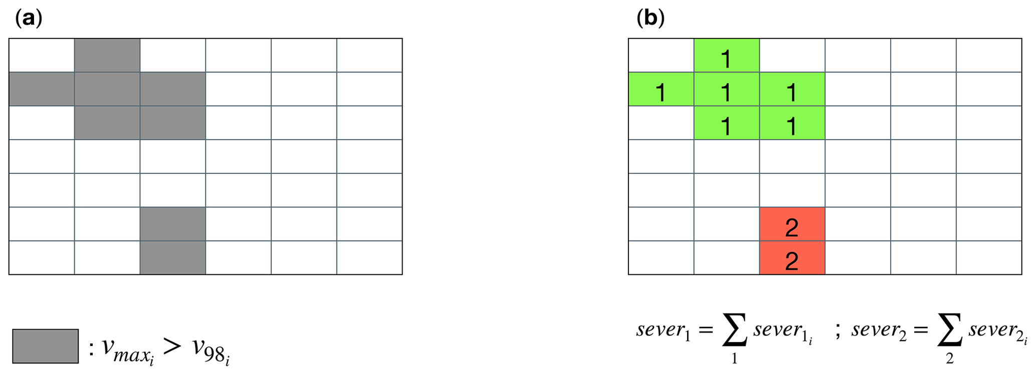
Figure 2Visual depiction of how 10 m wind footprints are identified. (a) To calculate values of severity on a given day, the daily maximum wind speed for each grid cell within the target region is calculated. Then, grid cells where the 10 m daily maximum wind speed has exceeded the local 98th percentile are selected (grey grid cells; there may be no such cells for a given day). (b) Last, connected regions of exceedances are found (green and red regions). Different connected regions are investigated separately. The value of severity for each region is the sum of values of severity of all grids cells within the region. The daily value of severity is equal to the largest single-region value.
The severity index we use was derived empirically to explain insured losses in Germany (Klawa and Ulbrich, 2003) and has chiefly been adopted for studying European windstorms. As such, it could be seen as unsuitable for the central Atlantic region. However, the index has a physical grounding since the cube of the wind speed represents the flux of kinetic energy. The index can be used to obtain a windstorm ranking even in a context where insured losses are irrelevant. Moreover, its use of a percentile threshold makes it appropriate to study extreme winds over a region such as the central North Atlantic where climatological wind values vary markedly.
It should be noted that the severity index we use to rank event intensity is sensitive to cyclone travelling speed. In particular, it favours fast-travelling cyclones, since they have more potential to exceed local 98th percentiles in a broader area inside the target region within a day. Very extreme but slowly moving cyclones would be down-ranked. As is shown later, top extremes are cyclones that travel rapidly because they are advected by a strong jet streak, which makes them more likely to be detected by the algorithm used here.
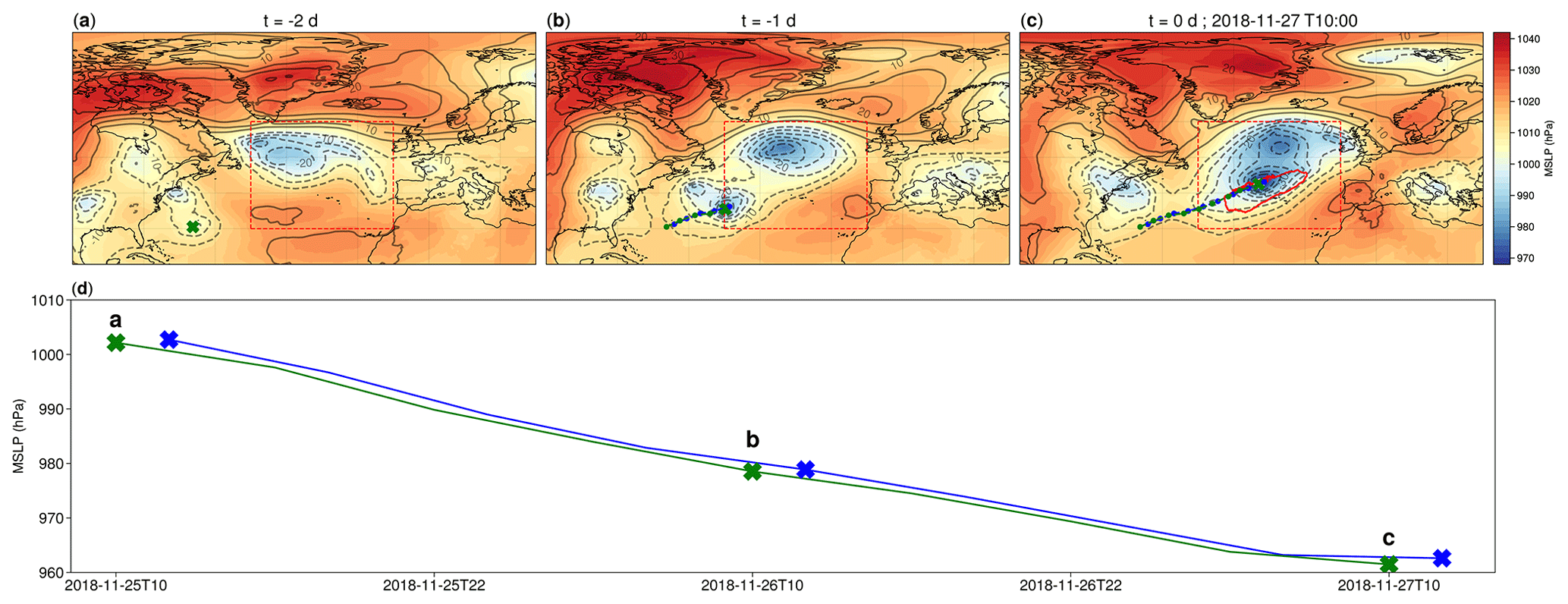
Figure 3MSLP field evolution of the extreme extratropical storm that reached peak 10 m wind speed on 27 November 2018 at 10:00 UTC (a–c). The location of the extreme cyclone centre at each time step is shown as a green cross. The thin dashed red boxes in each panel show the target region. Shading shows absolute MSLP; grey contours show MSLP anomalies relative to the 1950–2020 climatology, starting from ±5 hPa (dashed for negative anomalies). The wind footprint for the whole day of 27 November 2018 is shown as a thick red contour in panel (c). Tracks from Pinto et al. (2005) applied on ERA5 (dashed blue line) and manually obtained tracks (dashed green line) are shown in panels (b) and (c). MSLP evolution at the cyclone centre from using the two tracking methods is shown in panel (d), with the green crosses corresponding to the ones in panels (a)–(c) and blue crosses showing the closest time available from storm tracks by Pinto et al. (2005).
3.2 Detection and tracking of cyclones associated with the extreme 10 m winds
The basis for cyclone identification is a dataset of cyclone tracks computed using the cyclone tracking algorithm of Pinto et al. (2005), based on Murray and Simmonds (1991), and applied to the same ERA5 data used in this study. The algorithm identifies cyclones by first finding a maximum of MSLP Laplacian (a proxy for the maximum of relative vorticity) and then finding the MSLP minima closest to it. Tracks are further filtered to exclude weak, short-lived, and non-developing lows by applying the criteria from Pinto et al. (2009). As was shown in Neu et al. (2013), this tracking method performs well compared to other tracking schemes and has been used in numerous studies before (Gómara et al., 2014; Priestley et al., 2017, 2020; Leeding et al., 2023).
The cyclone track dataset from Pinto et al. (2005) was refined by additionally computing tracks of cyclones associated with the top 1 % of severity events using 1-hourly data, as described below. The main motivation behind this additional tracking is in the increased precision that it allows. As the tracks provided by the Pinto et al. (2005) algorithm are computed using 6-hourly data, the exact hour when the peak 10 m winds occurred could be missed by up to 5 h, yielding potentially large errors in the position of these fast-moving cyclones. We therefore refine the tracks by applying the following procedure. We first find the location of the peak 10 m wind speed within the strongest wind footprint for each day. After that, we identify the location of the cyclone associated with the event as the MSLP minimum closest to the peak wind speed location. The identification is performed at the time of day when 10 m wind speed is the strongest; in the composite analysis described below, this instant is taken as t=0. We then track every extreme cyclone back in time with an hourly time step by following the absolute MSLP minimum. For every hour before t=0, we put a box (± 4° latitude; +1°, −5° longitude) around the location of a cyclone at h step in time. To remove ambiguity in cases when several MSLP minima are close to each other, we perform a Gaussian smoothing of the MSLP field with a sigma of 0.1. We then look for an MSLP minimum within the box. As a check, we compare cyclone tracks obtained in this way with those produced by Pinto et al. (2005) and find no qualitative differences (an example of the refined tracks being more precise than tracks from Pinto et al. (2005) can be seen in Fig. 3b, c). We also performed a manual verification of the cyclone tracks by plotting the cyclone locations on MSLP maps (not shown). Tracks of the cyclones associated with the top 1 % of 10 m wind footprints are shown in Fig. 1.
The same tracking method was also used to track pre-existing downstream cyclones present after the cyclogenesis of the above top 1 % cyclones. These pre-existing cyclones are tracked from the time of cyclogenesis of the extreme cyclone (yellow triangle in the example in Fig. 1) up to 12 h before the peak 10 m wind speeds. Tracking after this time period proved to be less reliable since the proximity of two systems often seemed to produce multicentre cyclone-like structures (see Hanley and Caballero, 2012a).
Of the 115 events that make up the top 1 %, 16 are of tropical origin and match tracks from HURDAT, and we discard them from further analysis. The reason for discarding them is the large differences in development between purely extratropical cyclones and extratropical transitions. For example, we found that for the purely extratropical cyclones, cyclogenesis occurs around 2 d before the peak 10 m wind speed within the wind footprint (at d), while extratropical transitions have their origin much further back in time. Additionally, fields of upper-level PV and wind at 250 hPa show less coherence for extratropical transitions, thus making the composite analysis less useful. We hereafter refer to the remaining 99 purely extratropical events as top extremes. Top extremes are regularly interspersed through the 1950–2020 period, and there is no apparent trend in the frequency of their occurrences (see Appendix). It is interesting to note that the year 1999, which had many severe European windstorms (like Lothar), did not produce any events in the top-extreme class.
To assess features unique to top-extreme cyclones, we contrast them with a group of moderate extremes. This group consists of cyclones in the same target region but associated with the bottom 10 % of events with non-zero severity. These are cyclones that cause local exceedances of 98th percentiles but by a modest amount. To facilitate the comparison between moderate- and top-extreme cyclones, we only select the moderate extremes that had valid tracks for at least 2 d before the occurrence of peak 10 m wind speed in the target region (as is typical for top extremes). We find moderate extremes in tracks based on Pinto et al. (2005), as the greater number of events requires a more efficient search of cyclones identified in ERA5 compared to the tracking done backwards from the moment of maximum 10 m winds, as was done for top extremes. Since the search for moderate extremes also includes pre-defined criteria, the total number of cyclones found that satisfy it is lower than the number of moderate-extreme days. At the end, we obtain 117 moderate extremes matching our criteria, a number of the same order of magnitude as the number of top extremes. Because of the difference in the detection of top-extreme and moderate-extreme events, we use 1-hourly and 6-hourly tracks for them, respectively.
The choice of cyclone tracking method we used could potentially impact the results. However, alternative tracking based on a different variable (like surface vorticity) should not substantially impact the tracks of top extremes. As was shown in tracking intercomparison studies (like those by Neu et al., 2013; Ulbrich et al., 2013b), different tracking algorithms tend to agree well for deeper, more developed cyclones like top extremes. A similar result was also obtained in a more recent study by Messmer and Simmonds (2021), where two different tracking methods were used to study compound extreme wind and precipitation events. Additionally, a bias towards slower-moving cyclones intrinsic to methods based on MSLP (Sinclair, 1994) should be less prominent when using 1-hourly tracks as the box within which we search for MSLP minima between the time steps covers a distance larger than 60–70 km, which the fastest-moving cyclones cover in an hour (Neu et al., 2013). Differences between the tracking methods could, however, be more important for the set of moderate extremes as cyclones in this group have a pre-defined condition of having cyclogenesis at least 2 d before the peak 10 m wind speeds in the target region. Since one of the biggest differences between the tracking methods lies in the identification of the time of cyclogenesis, with vorticity-based methods tending to identify cyclogenesis earlier (Neu et al., 2013), the group of moderate extremes could potentially be larger if a different cyclone tracking method was employed.
3.3 Composite analysis
We perform a composite analysis to study the typical large-scale features associated with our two groups of cyclones. We use both cyclone- and location-centred composites to study meteorological variables of interest (like PV, MSLP, and wind at 250 hPa). Because 1° of longitude spans a distance that varies with latitude, compositing on latitude–longitude regions would introduce a distortion. We thus perform the composites after regridding meteorological fields to radial grids centred on the cyclone centres or locations of interest in the case of location-centred composites. With this aim, we apply the method from Bengtsson et al. (2007) (described in detail in their Appendix A), which has previously been used in other studies for similar purposes (for example Dacre et al., 2012; Laurila et al., 2021a; Dolores-Tesillos et al., 2022).
Most of the composite fields we show are the anomalies of meteorological fields from 1950 to 2020 climatology. To get the climatologies, we first calculate the daily means for calendar days of each variable for every grid point and at every level of interest. Then, we obtain climatologies by computing a 31 d running mean from these datasets.
3.4 Pressure tendency equation analysis
Since cyclones within the two selected groups experience surface MSLP decrease in the days leading to their peak 10 m winds (as is shown in Sect. 4.2), we apply the pressure tendency equation analysis to determine the main contributors to the surface MSLP decrease in top and moderate extremes between and t=0. This approach analyses the expanded pressure tendency equation as described in Fink et al. (2012) and Pirret et al. (2017). Most cyclones are predominantly driven by a combination of diabatic processes (radiation, latent heating) and baroclinic conversion (rising of warm air which moves polewards and sinking of cold air which moves equatorwards). The pressure tendency equation decomposes the contribution of these processes by reformulating the classical pressure tendency equation and introducing virtual temperature as the main variable.
In practice, the pressure tendency equation analysis takes 6-hourly tracks of cyclones and evaluates each term of the pressure tendency equation by following a vertical column of air over a 3°×3° latitude–longitude box centred on the surface cyclone centre. The equation has the following form:
where psfc is surface pressure, ρsfc is surface air density, ϕp2 is geopotential at the upper boundary p2, Rd is the gas constant for dry air, Tv is virtual temperature, g is gravitational acceleration, E is evaporation, P is precipitation, and RESPTE is residuum. As Eq. (2) shows, the tendency of the surface pressure is equal to the sum of the change in geopotential at the upper boundary (100 hPa in this study, which was found to be the most sensible choice for extratropical cyclones by Fink et al., 2012); the vertically integrated virtual temperature tendency; the mass change caused by the difference between evaporation and precipitation; and residual due to the errors from vertical integration, discretisation, or the data model itself. Therefore, if the column of air does not change its height, its warming will cause horizontal expansion, divergence of air, and loss of mass. The end result of this process will be a surface pressure fall. Similarly, if nothing but the upper boundary of the column changes, its lowering will cause pressure decrease.
The vertically integrated virtual temperature tendency in the pressure tendency equation can be expanded in the following way:
where v and ω are the horizontal and vertical wind components, cp is the specific heat capacity at constant pressure, and Q is the diabatic heating rate. Expansion of the vertically integrated virtual temperature tendency term allows the pressure tendency equation to contain terms that represent horizontal temperature advection (interpreted as “baroclinic” contribution; the first term on the RHS of Eq. 3), vertical motion (which typically causes surface pressure increases; the second term on the RHS of Eq. 3), and the diabatic term. Since ERA5 does not contain the diabatic heating rate products, the diabatic term (the third term on the RHS of Eq. 3) is calculated as a residual from subtracting the horizontal temperature advection and vertical motion terms from the vertically integrated virtual temperature tendency, all of which are calculated explicitly. For more details about the pressure tendency equation approach, see Fink et al. (2012).
4.1 Example of an extreme cyclone
An illustrative example from the set of top extremes is shown in Fig. 3, which presents the MSLP evolution from the time of cyclogenesis until the time of peak 10 m wind speed for the selected event. Around 2 d before the cyclone caused the extreme 10 m winds in the target region (27 November 2018 at 10:00 UTC), the system originated along the east coast of North America as a shallow depression (Fig. 3a). At the time of the cyclogenesis there was a pre-existing, well-developed cyclone situated south of Greenland. This pre-existing downstream cyclone remained in the target region during the explosive deepening of the extreme cyclone during the next 2 d. Once the extreme cyclone reaches the target region, it produces a large extreme wind footprint along the track (Fig. 3c). During this day, the extreme and the pre-existing cyclones appear to merge, forming a broad area of low MSLP that can be classified as a multicentre cyclone (Hanley and Caballero, 2012a). The interaction between the pre-existing and the extreme cyclone shown in this example is common to all events belonging to the top-extreme group (see composites in Sect. 4.2 below).
4.2 Composite analysis of extreme events
Composite MSLP anomalies centred on the top extremes and moderate extremes are shown in Fig. 4. Like in the example above, there are pre-existing downstream cyclones to the northeast of the top extremes around the time of their cyclogenesis (Fig. 4a). At this time both lows have anomalies of up to 10 hPa. As time proceeds, the top-extreme cyclones deepen and approach the pre-existing downstream cyclones. At the time of peak 10 m wind speeds (t=0, Fig. 4c), the two systems have merged in the composite. Negative MSLP anomalies also reach their minimum, with anomalies exceeding −35 hPa. The rapid deepening of top-extreme cyclones that occurs as they approach the pre-existing downstream cyclones is in line with the result that the majority of top extremes (87 out of 99 – or 88 %) is explosively deepening cyclones with the normalised values of the 24-hourly pressure decrease greater than 24 hPa (the criteria used in Sanders and Gyakum, 1980).
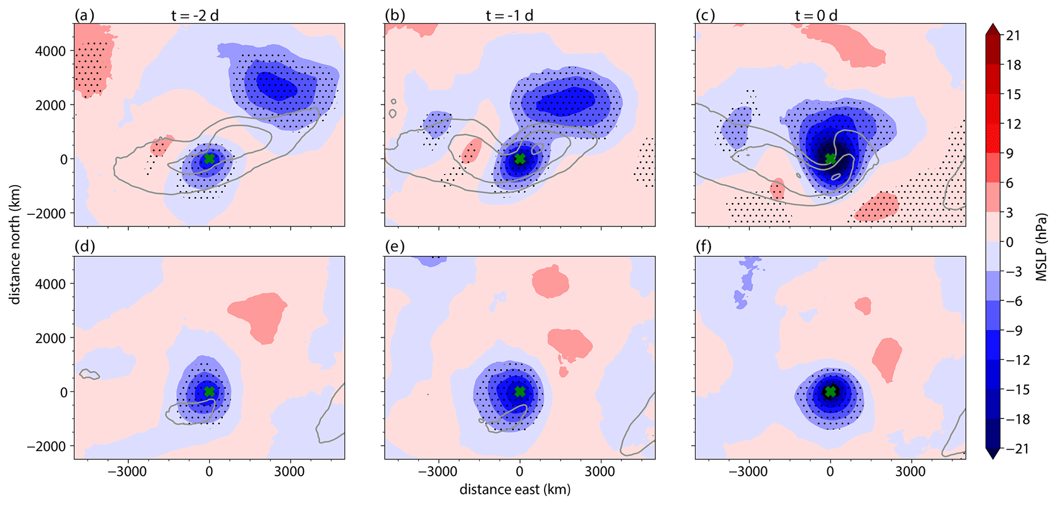
Figure 4Composite MSLP anomalies relative to the 1950–2020 climatology for top extremes (a–c) and moderate extremes (d–f), centred on the cyclone locations from to t=0 d. Lags are relative to the time of maximum 10 m wind speeds on the day with maximum severity. The green crosses denote locations of top- and moderate-extreme cyclone centres. The black dots show areas where MSLP anomalies are statistically significant at the 1 % level computed with Monte Carlo sampling (150 samples, each made from averaging 99 and 117 samples for top and moderate extremes, respectively) and corrected for false discovery (Wilks, 2016). The grey contours show the values of 250 hPa wind speeds, starting from 30 ms−1 and increasing in steps of 10 ms−1.
On the other hand, composites of moderate-extreme cyclones (Fig. 4d–f) reveal an absence of pre-existing downstream cyclones at d. In fact, a weak positive MSLP anomaly with values lower than 5 hPa is found in the region where pre-existing cyclones are present for top extremes. Therefore, the presence of the pre-existing downstream cyclones appears to be an essential feature in generating top extremes.
Top-extreme cyclones are also associated with an anomalously strong jet streak from to t=0 d (Fig. 4a–c). The cyclones cross the jet streak from d when they are located around the right-entrance region of the jet to t=0 d when they are in the left-exit region of the jet. Right-entrance and left-exit regions of the jet streak are associated with strong upper-level divergence, which makes them favourable for the intensification of cyclones (see for example Uccellini, 1990; Rivière et al., 2010). The absolute values of composite wind speed at 250 hPa for top extremes are over the broad regions where the wind speed exceeds 40 ms−1 (Fig. 4a–c).
Figure 5 shows the evolution of upper-level fields corresponding to the surface composites in Fig. 4. Positive upper-level PV anomalies associated with top-extreme and pre-existing downstream cyclones after the cyclogenesis are shown in Fig. 5a–c; 2 d before the peak 10 m wind, there is a well-defined, zonally extended area of positive PV anomalies stretching to the northeast of the developing extreme cyclone (Fig. 5a). At the same time, wind speed anomalies at 250 hPa show cyclonic upper-level winds around the pre-existing downstream cyclone. This cyclonic flow is organised so as to advect high-PV air southward, helping promote positive PV anomalies at the location of the top-extreme cyclone. As the top-extreme cyclone moves closer to the pre-existing downstream cyclone, positive upper-level PV anomalies associated with the two systems merge into a broader area of statistically significant positive PV anomalies. The intensity of the anomalies increases from to t=0. At t=0, when the two composite systems have fully merged and surface winds reach their peak, upper-level PV anomalies reach a maximum of over 3 pvu.
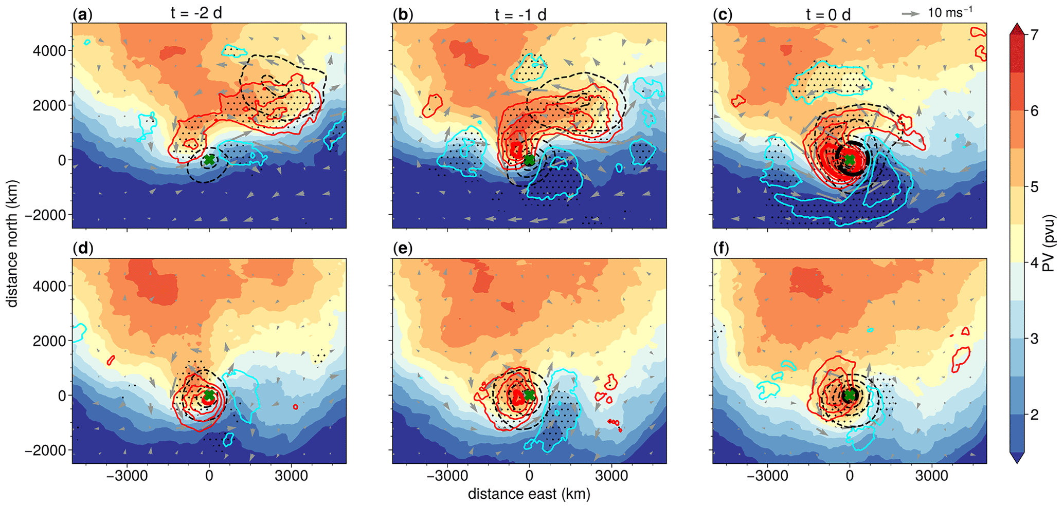
Figure 5Upper-level composites for top extremes (a–c) and moderate extremes (d–f), centred on the cyclone locations from d to t=0 d. The colours show upper-level PV (200–300 hPa mean) values, while the red and blue contours show positive and negative upper-level PV anomalies relative to the 1950–2020 climatology, respectively, starting from ±0.5 pvu, with thick contours at ±2 pvu. The black dots show areas where upper-level PV anomalies are statistically significant at the 1 % level, computed as in Fig. 4. The grey arrows show 250 hPa wind speed anomalies from climatology. The black contours show MSLP anomalies relative to the 1950–2020 climatology, starting from ±5 hPa (dashed for negative anomalies), with thick contours at ±20 hPa. The green crosses have the same meaning as in Fig. 4.
The moderate extremes (Fig. 5d–f) display a small downstream region with positive upper-level PV anomalies, yet these are not statistically significant and are not connected with a surface low. Large positive upper-level PV anomalies are confined to the area around the extreme cyclone itself and never exceed 2 pvu even at t=0. Consistently, wind speed anomalies at 250 hPa (Fig. 5d–f) are weaker than those shown in Fig. 5a–c, and substantial anomalies are only present in the region around the surface low. Absolute values of the jet streak at 250 hPa are much weaker for moderate- than for top-extreme cyclones (Fig. 4), making the jet streak less able to facilitate intensification of the cyclone. It should also be mentioned that PV anomalies at t=0 d averaged in a circle with a radius of 300 km around the cyclone centres reveal that the two groups also differ in the strength of the lower-level PV anomaly. Top-extreme cyclones have a larger median of positive PV anomalies from 900 to 200 hPa (see Appendix), which agrees with the previous findings by Čampa and Wernli (2012).
To investigate the conditions leading to the development of extremes prior to their time of cyclogenesis, we compute lagged composites centred on the location of cyclogenesis (Fig. 6). At d before cyclogenesis, the composite for top extremes (Fig. 6a) shows a broad lobe of high PV directly to the north of the cyclogenesis location. Considering that cyclogenesis in all cases occurs near the east coast of North America, this lobe is consistent with the regional PV climatology, which features a high-PV lobe over Hudson Bay (Fig. 1; mean location of top-extreme cyclogenesis is marked by a green cross). The composite PV field also displays a moderate positive PV anomaly to the east of the cyclogenesis location, which corresponds to a surface MSLP anomaly. Both persist and strengthen in subsequent days (Fig. 6b, c) and can be identified as the pre-existing cyclone discussed above. This upper-level PV anomaly results from a deformation of the climatological PV structure reminiscent of cyclonic Rossby wave breaking, which has been robustly identified as a precursor of extreme North Atlantic cyclones in previous work (Hanley and Caballero, 2012b; Gómara et al., 2014).
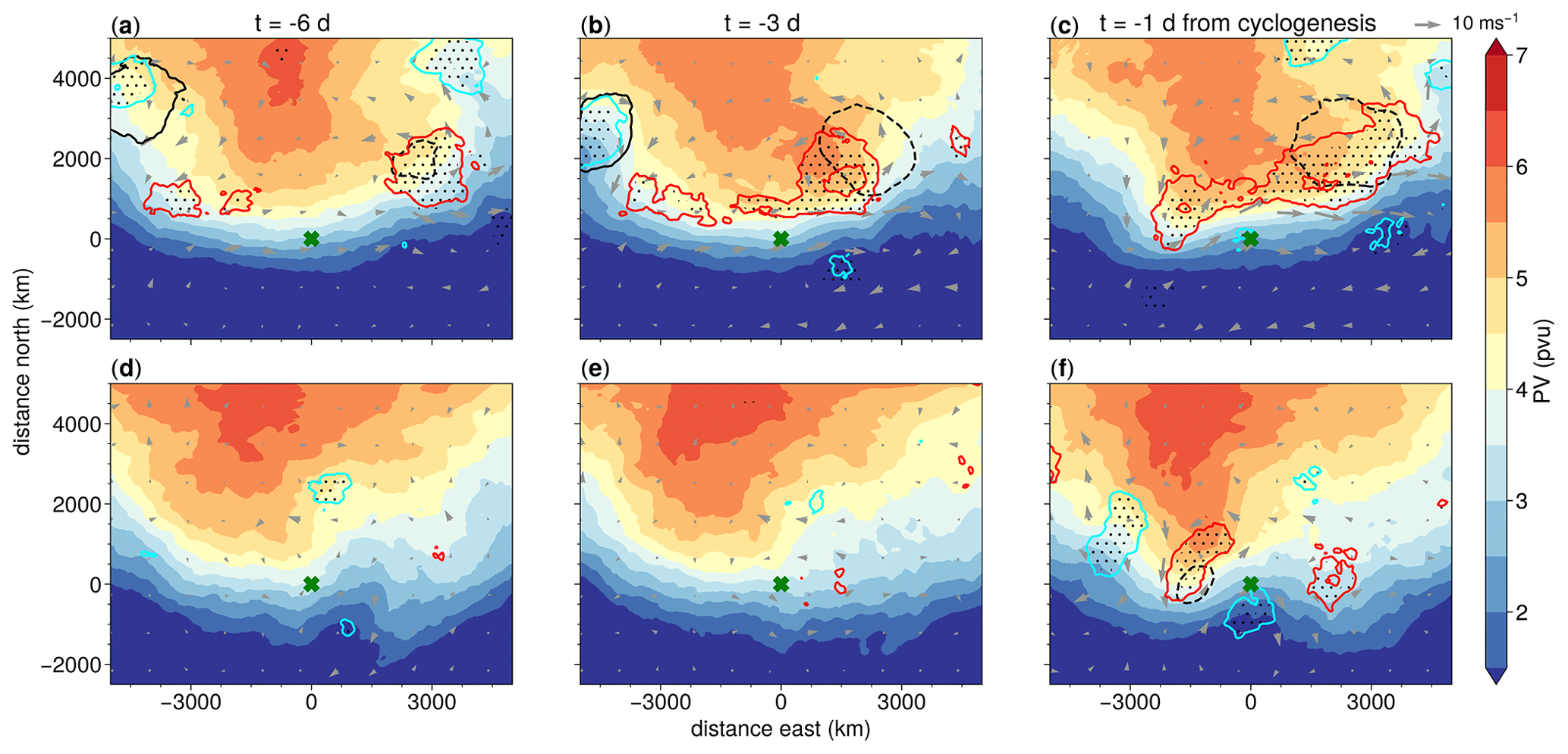
Figure 6Composites centred at the locations of cyclogenesis of top extremes (a–c) and moderate extremes (d–f). Lags are relative to the time of cyclogenesis. The colours, contours, crosses, and dots have the same meaning as in Fig. 5.
In addition, at d a positive PV anomaly appears to the west of the cyclogenesis location. This anomaly has no surface footprint, suggestive of an open-wave upper-level anomaly which in subsequent days propagates eastward until it reaches the location of cyclogenesis off the east coast of North America. Thereafter, it becomes the upper-level component of the extreme cyclone (Fig. 5a–c). In fact, from d before cyclogenesis (Fig. 6b), a band of positive PV anomalies stretches between the incipient top-extreme cyclone and the pre-existing downstream cyclone. This band can be identified after cyclogenesis as corresponding to the jet streak seen in Fig. 4a.
Turning to moderate extremes (Fig. 6d–f), we see that 6 and 3 d before cyclogenesis there are no statistically significant MSLP anomalies, while upper-level PV anomalies are confined to small regions, and anomalies of wind speed at 250 hPa are much weaker and less organised compared to top extremes. MSLP and upper-level PV and wind anomalies only strengthen 1 d before cyclogenesis (Fig. 6f) and are associated with the moderate-extreme cyclone itself: while there is a region of positive PV anomalies to the east of the incipient moderate-extreme cyclone, it has no surface footprint and is absent in subsequent days. Thus, as discussed above, the main difference between top and moderate extremes is that the latter lacks a well-organised, persistent pre-existing downstream cyclone to the east of the incipient cyclone.
4.3 Pressure tendency equation analysis
In this section we take a different perspective and quantitatively compare the mechanisms leading to deepening of top and moderate extremes using the surface pressure tendency decomposition approach. Figure 7 shows contributions of each term in the pressure tendency equation averaged over the 2 d, leading to the peak 10 m wind speed for both cyclone groups. The vertical velocity term leads to surface pressure increase, i.e. to a weakening of the surface cyclone. Horizontal temperature advection – the baroclinic term – is negative (strengthens the cyclone) and slightly smaller in magnitude than the vertical velocity term. The absolute values of both terms are larger for top extremes than for moderate extremes (Fig. 7), which is one difference between the groups.
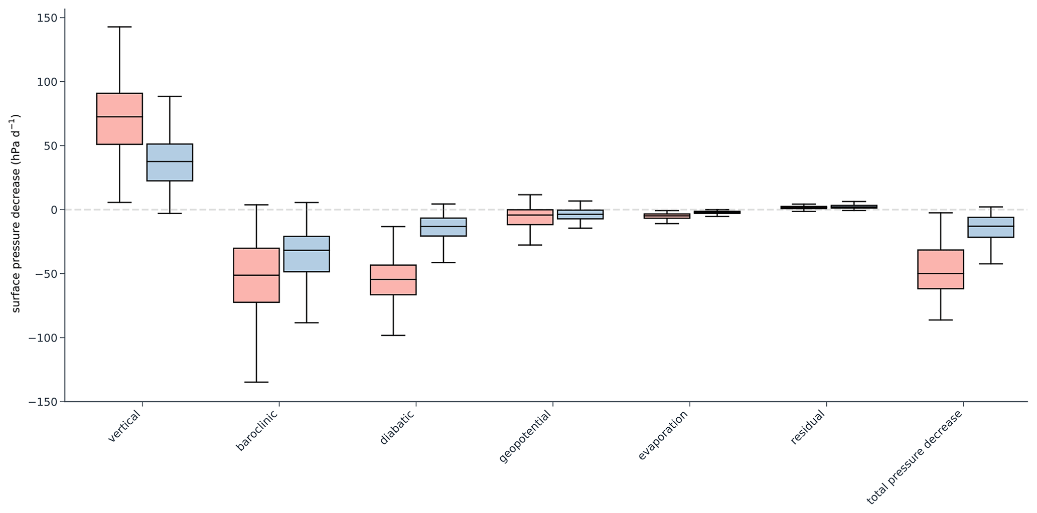
Figure 7Boxplots of contributions of each term of the pressure tendency equation to pressure decrease for top extremes (red boxes) and moderate extremes (blue boxes). The boxes show interquartile ranges, and the horizontal black lines in each box show a median. All terms are averaged over the 2 d up to the time of maximum 10 m wind speed.
The largest difference between the groups lies in the pressure decrease caused by the diabatic term. The diabatic term for moderate extremes is around half of the baroclinic term. For top extremes, the diabatic term is as large as the baroclinic term. With both terms being larger than for the moderate extremes, the total surface pressure drop for top extremes is around twice as large. For all of these terms (vertical, baroclinic, diabatic, and total pressure decrease), the mean values of top extremes are statistically different from moderate extremes at the 95 % confidence level according to the Wilcoxon signed rank test.
Figure 7 also shows that other terms in the pressure tendency equation (the geopotential term and the term that arises from changes in mass due to the difference between evaporation and precipitation) are on average of minor importance for cyclone intensification. The residual for the selected storms is also close to zero, implying that the decomposition accurately captures the drivers of the observed surface pressure drop.
On an individual storm level, the pressure tendency equation analysis shows a large variability in the influence of the different terms, as can be seen from uncertainty ranges in Fig. 7. Even considering uncertainties, common features for both groups are a small influence of the evaporation and precipitation term, a vertical term which increases the surface pressure, and the dominance of either baroclinic or diabatic terms for cyclone development. Which one of the latter two is the leading driver of surface pressure fall, however, changes from storm to storm. This is in line e.g. with the results of Pirret et al. (2017), who found a wide range of the different contributions to cyclone deepening.
For top-extreme cyclones, a slightly larger group of cyclones is primarily driven by diabatic processes compared to baroclinic processes (41 versus 35, respectively). The rest of the cyclones in the group have a difference between diabatic and horizontal temperature advection smaller than 5 % (the criterion we used to identify predominantly diabatic or baroclinic storms). Separate composites for diabatic versus baroclinic cyclones show no evident qualitative differences from the composites for all top extremes, even when imposing a 10 % difference between the two terms to identify the cyclones (not shown).
As the top extremes occur over a period under which the signal of climate change has become more prominent, it is relevant to investigate potential trends in the surface pressure tendency terms. To do this, we divide the events into two sub-periods – one from 1950–1985 and the other from 1986–2020 – with the difference between the two periods providing evidence for a warming-related trend. Comparison of pressure tendency equation analysis for two periods shows that there is a statistically significant increase in the diabatic contribution to surface pressure decrease and in the total surface pressure decrease in the warmer period (at the 95 % confidence level according to the Wilcoxon signed rank test) (see appendices). There is also an increase in the baroclinic contribution, though it is not statistically significant. Moderate extremes, on the other hand, do not show any significant changes between the periods, suggesting that the most extreme cyclones are most sensitive to warming.
The above analysis shows that the presence of a pre-existing downstream cyclone is the key feature distinguishing top-extreme from moderate-extreme cyclones. A composite analysis of top-extreme cases shows a gradual build-up of positive upper-level PV anomalies to the north of the cyclogenesis locations. After cyclogenesis and before the peak 10 m winds, top-extreme cyclones cross the jet streak while approaching the pre-existing downstream cyclone. At the time of peak 10 m winds, there is a merging of top-extreme and pre-existing cyclones, as their MSLP and positive upper-level PV anomalies form a joint large-scale system. On the other hand, the development of moderate-extreme cyclones generally occurs in the absence of pre-existing downstream cyclones, both before and after their cyclogenesis. The jet and the upper-level PV anomalies are weaker for moderate-extreme cyclones, as are the negative MSLP anomalies at the time of their peak 10 m wind speeds.
Pre-existing downstream cyclones may favour the intensification of top-extreme cyclones in at least two ways. One is through the intensification of the jet streak. Upper-level PV composites show a pattern reminiscent of cyclonic Rossby wave breaking in the days before the genesis of top-extreme cyclones (Fig. 6b). Before cyclogenesis, pre-existing downstream cyclones are situated just to the east of the climatological high-PV reservoir centred over Hudson Bay. Wind anomalies at 250 hPa associated with pre-existing downstream cyclones favour southward advection of high-PV air, generating positive PV anomalies, strengthening PV gradients, and generating strong jet anomalies. As shown in previous work, positive jet anomalies are associated with rapidly intensifying cyclones over the North Atlantic (e.g. Gómara et al., 2014) due to strong upper-level divergence in the jet's right-entrance and left-exit regions. Another reason why the presence of pre-existing downstream cyclones could be important is through direct cyclone–cyclone interactions and merging of the extreme and pre-existing cyclones. In particular, Fig. 5a–c suggest that the two cyclones become intertwined and combine their PV to yield a very strong upper-level PV anomaly, which is typically associated with very intense MSLP anomalies (Čampa and Wernli, 2012). The precise dynamics of this merging process and of the cyclone–jet streak interaction mentioned above provide interesting avenues for future research.
The situation where one cyclone develops to the southwest of another pre-existing downstream cyclone, as seen for the top extremes, is reminiscent of cyclone families and secondary cyclogenesis, a concept originating from Bjerknes and Solberg (1922). Composite analysis, however, is not the best tool for judging whether top-extreme cyclones are secondary cyclones because of the smoothing of fields intrinsic to the compositing. Answering this question would require investigating each extreme cyclone individually and assessing its relation to a trailing cold front generated by the pre-existing cyclone (for example using the metrics of Priestley et al., 2020), which is another possible direction for future work.
We also analysed the development of top- and moderate-extreme cyclones using the pressure tendency decomposition framework. Despite large storm-to-storm variability in the relative size of the terms in the pressure tendency equation, in line with Fink et al. (2012) and Pirret et al. (2017), comparison of the factors that drive the deepening of storms between the two cyclone groups identified here reveals a systematically greater influence of the diabatic term for top-extreme cyclones than for moderate cyclones. All the leading terms have greater absolute values for top-extreme cyclones, but the diabatic term has a greater relative importance as well compared to the baroclinic term. One possible explanation could be that stronger storms have greater vertical velocities, which, all else being equal, would imply an increase in condensation rates and diabatic heating. However, it remains unclear whether the increase in the absolute baroclinic contribution (that is also seen for top-extreme cyclones) drives the increase in the diabatic contribution or if the opposite is the case.
There are several ways in which this study could be expanded to further understand cyclones that cause extreme 10 m wind over the ocean. Investigating whether the mechanisms identified here are important in other ocean basins (North Pacific and Southern Ocean) is an obvious next step. This could also include investigation of long-term trends in storminess, along the lines of Feser et al. (2015). To quantify connections between the PV anomalies, 10 m wind speeds, and cyclone–cyclone interactions identified here, a different kind of analysis would need to be performed, such as PV inversion analysis or idealised modelling studies. Additionally, near-surface winds occur in the boundary layer, which makes them a multi-scale phenomenon involving mesoscale and turbulence-scale processes. As this study only investigates large-scale dynamics that favour extreme 10 m winds, one route of further research could delve deeper into the mesoscale processes associated with these systems to provide linkages that connect large-scale physics with boundary layer physics. Such studies could implement tools used to detect sting jets (like, for example, those in Manning et al., 2022; Hart et al., 2017), a mesoscale phenomenon that has repeatedly been linked to extreme near-surface winds (see for example Hewson and Neu, 2015) and is not addressed in this study. Future studies with a focus on boundary layer processes could also investigate how mechanisms known to influence PV in the boundary layer, like creation of PV with latent heating along the warm conveyor belt or destruction of it through heat fluxes in the cold sectors (as shown in Plant and Belcher, 2007), act in the case of top-extreme cyclones.
We provide a large-scale perspective on extreme near-surface winds in the central North Atlantic. We select cyclones associated with the top 1 % of extreme 10 m wind events during boreal winter, top extremes, and compare them with a group of moderate extremes – cyclones that also cause strong winds but with weaker footprints. We analyse both groups of cyclones through time-lagged composites and through the surface pressure tendency decomposition. We aim to determine the large-scale circulation features favouring the development of top extremes. We find that a key feature of top extremes is the presence of a pre-existing cyclone to the northeast of the developing cyclone. These pre-existing downstream cyclones can be identified at least 6 d prior to genesis of top-extreme cyclones but are generally absent for more moderate extremes.
The genesis of top-extreme cyclones occurs around 2 d before they reach peak severity. The pre-existing downstream cyclones help to generate a jet streak to the east of the incipient top-extreme cyclones. As top-extreme cyclones develop, they cross this jet streak and experience explosive deepening and intensification of upper-level PV anomalies. The pressure tendency equation analysis shows that the main difference between these top extremes relative to moderate extremes is the significantly larger median contribution of diabatic processes to cyclone growth in top extremes. Although there is a large variation in the relative role of the terms contributing to surface deepening from storm to storm, all the leading terms in the pressure tendency equation have, on average, larger absolute values for top extremes.
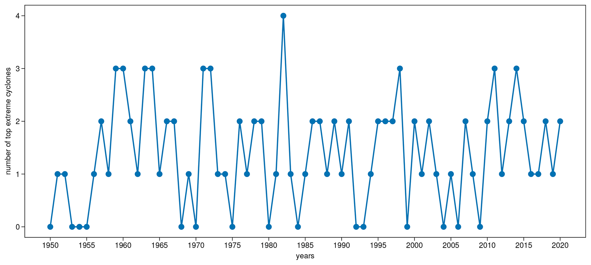
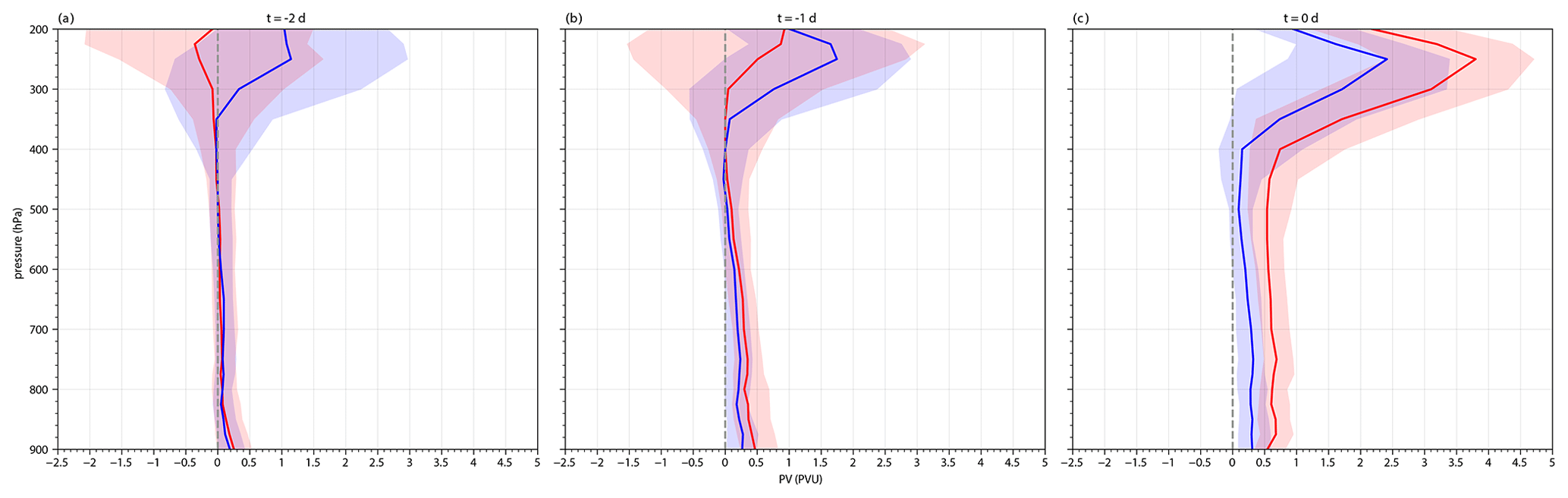
Figure A2Median of PV anomalies from 1950–2020 climatology averaged at all available ERA5 pressure levels from 900 to 200 hPa in a circle with a radius of 300 km around cyclone centres of top extremes (red lines) and moderate extremes (blue lines). The shading shows interquartile ranges.
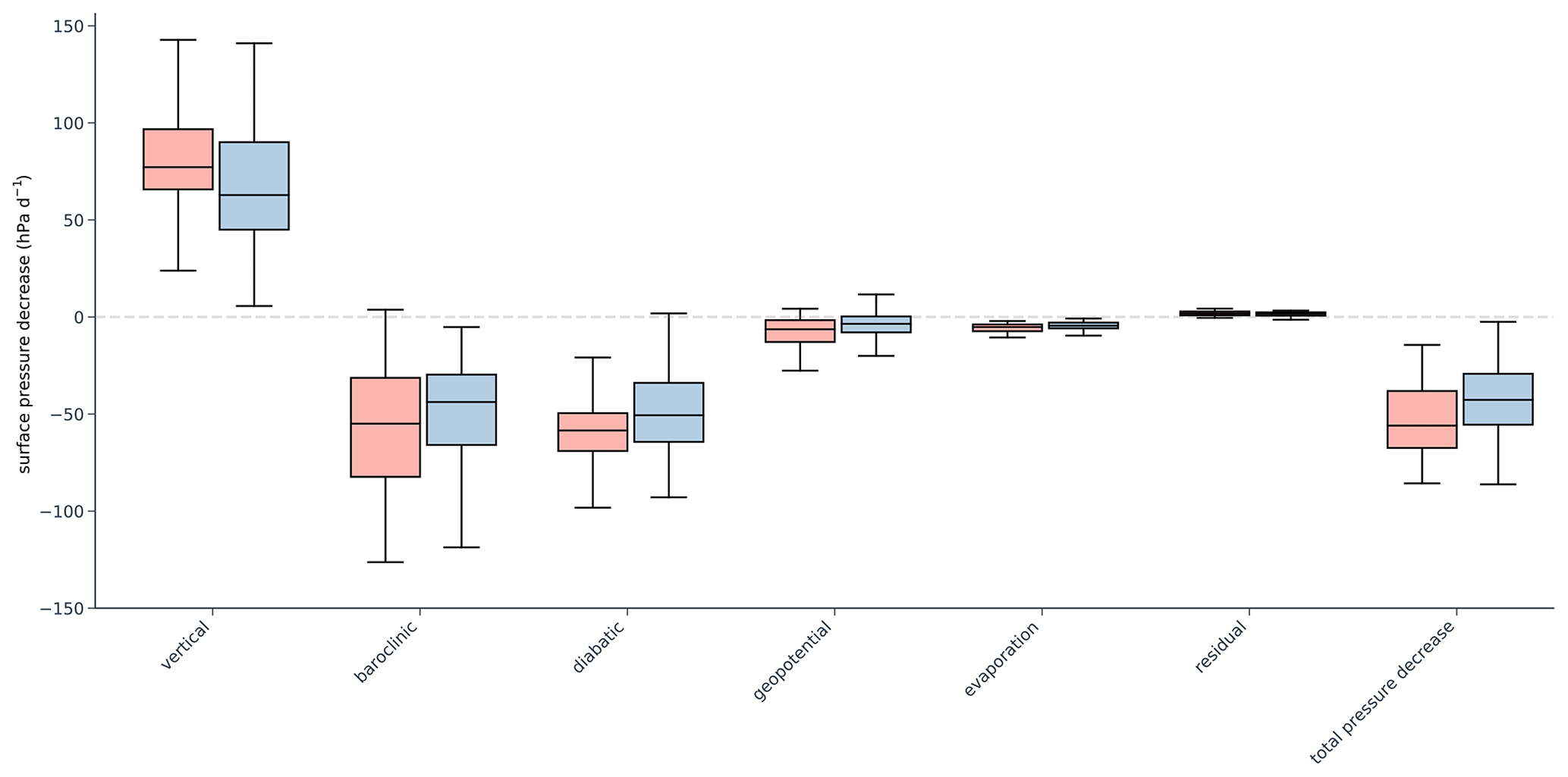
Figure A3Boxplots of contributions of each term of the pressure tendency equation to pressure decrease for top extremes that occurred from 1950–1985 (blue boxes) and top extremes that occurred from 1986–2020 (red boxes). Boxes have the same meaning as in Fig. 7. Diabatic contribution and total pressure decrease are the only terms that show a statistically significant difference between the two groups at the 95 % confidence level according to the Wilcoxon signed rank test.
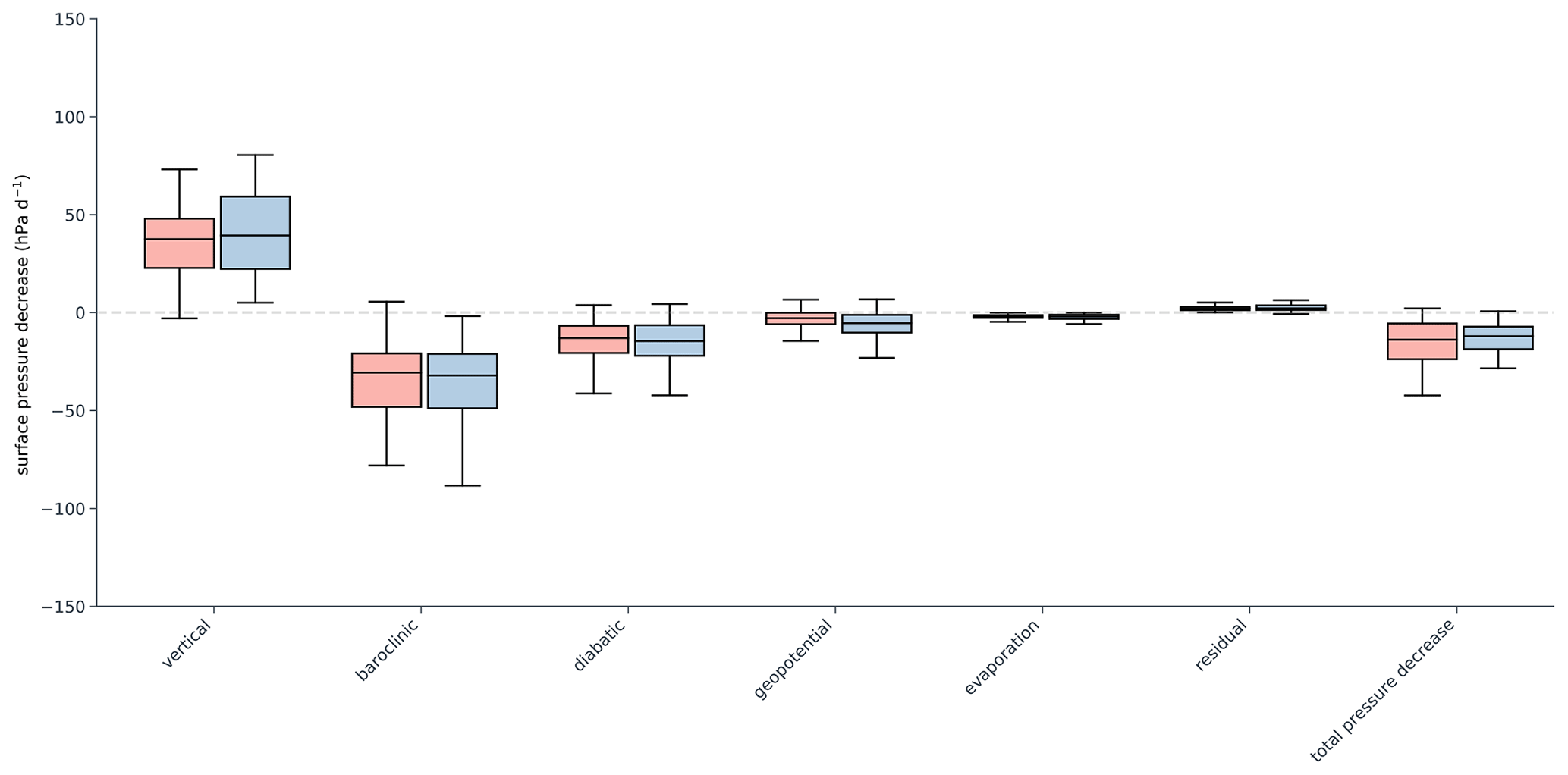
Figure A4Boxplots of contributions of each term of the pressure tendency equation to pressure decrease for moderate extremes that occurred from 1950–1985 (blue boxes) and moderate extremes that occurred from 1986–2020 (red boxes). Boxes have the same meaning as in Fig. 7. There are no terms that show a statistically significant difference between the two groups at the 95 % confidence level according to the Wilcoxon signed rank test.
The ERA5 reanalysis data used in this study can be downloaded from https://cds.climate.copernicus.eu/cdsapp#!/dataset/reanalysis-era5-pressure-levels?tab=form (last access: 26 March 2024) (Hersbach et al., 2023). We have also downloaded parts of ERA5 data from the Research Data Archive at the Computational and Information Systems Laboratory of the National Center for Atmospheric Research (https://doi.org/10.5065/BH6N-5N20) (European Centre for Medium-Range Weather Forecasts, 2019). Storm tracks found in ERA5 using the algorithm from Pinto et al. (2005) and the code used for this analysis are available upon request.
AS, RC, and GM designed the study. AS carried out the analysis and drafted the first version of the manuscript. RC, GM, and JGP provided methods and data. All authors contributed to discussions, structuring the analysis, and reviewing the paper.
The contact author has declared that none of the authors has any competing interests.
Publisher’s note: Copernicus Publications remains neutral with regard to jurisdictional claims made in the text, published maps, institutional affiliations, or any other geographical representation in this paper. While Copernicus Publications makes every effort to include appropriate place names, the final responsibility lies with the authors.
We thank the two anonymous reviewers for their constructive comments on the paper.
This research has been supported by the Horizon 2020 framework programme H2020 Excellent Science (Marie Skłodowska-Curie grant agreement no. 956396, EDIPI project). Joaquim G. Pinto thanks the AXA Research Fund for support.
This paper was edited by Shira Raveh-Rubin and reviewed by two anonymous referees.
Bengtsson, L., Hodges, K. I., Esch, M., Keenlyside, N., Kornblueh, L., Luo, J.-J., and Yamagata, T.: How may tropical cyclones change in a warmer climate?, Tellus A, 59, 539–561, 2007. a
Berz, G.: Windstorm and storm surges in Europe: loss trends and possible counter-actions from the viewpoint of an international reinsurer, Philos. T. R. Soc. A, 363, 1431–1440, 2005. a
Bjerknes, J. and Solberg, H.: Life cycle of cyclones and the polar front theory of atmospheric circulation, Grondahl, Geofys. Publ., 1–18, 1922. a
Čampa, J. and Wernli, H.: A PV perspective on the vertical structure of mature midlatitude cyclones in the Northern Hemisphere, J. Atmos. Sci., 69, 725–740, 2012. a, b, c, d
Campos, R. M., Gramcianinov, C. B., de Camargo, R., and da Silva Dias, P. L.: Assessment and calibration of ERA5 severe winds in the Atlantic Ocean using satellite data, Remote Sens., 14, 4918, https://doi.org/10.3390/rs14194918, 2022. a, b
Cardone, V., Callahan, B., Chen, H., Cox, A., Morrone, M., and Swail, V.: Global distribution and risk to shipping of very extreme sea states (VESS), Int. J. Climatol., 35, 69–84, 2015. a
Chen, T.-C., Collet, F., and Di Luca, A.: Evaluation of ERA5 precipitation and 10-m wind speed associated with extratropical cyclones using station data over North America, Int. J. Climatol., 44, 729–747, https://doi.org/10.1002/joc.8339, 2024. a
Dacre, H., Hawcroft, M., Stringer, M., and Hodges, K.: An extratropical cyclone atlas: A tool for illustrating cyclone structure and evolution characteristics, B. Am. Meteorol. Soc., 93, 1497–1502, 2012. a
Dacre, H. F. and Gray, S. L.: The spatial distribution and evolution characteristics of North Atlantic cyclones, Mon. Weather Rev., 137, 99–115, 2009. a
Dacre, H. F. and Pinto, J. G.: Serial clustering of extratropical cyclones: A review of where, when and why it occurs, NPJ Climate and Atmospheric Science, 3, 48, https://doi.org/10.1038/s41612-020-00152-9, 2020. a
de León, S. P. and Bettencourt, J.: Composite analysis of North Atlantic extra-tropical cyclone waves from satellite altimetry observations, Adv. Space Res., 68, 762–772, 2021. a
Dolores-Tesillos, E., Teubler, F., and Pfahl, S.: Future changes in North Atlantic winter cyclones in CESM-LE – Part 1: Cyclone intensity, potential vorticity anomalies, and horizontal wind speed, Weather Clim. Dynam., 3, 429–448, https://doi.org/10.5194/wcd-3-429-2022, 2022. a, b
Earl, N., Dorling, S., Starks, M., and Finch, R.: Subsynoptic-scale features associated with extreme surface gusts in UK extratropical cyclone events, Geophys. Res. Lett., 44, 3932–3940, 2017. a
European Centre for Medium-Range Weather Forecasts: updated monthly. ERA5 Reanalysis (0.25 Degree Latitude-Longitude Grid), Research Data Archive at the National Center for Atmospheric Research, Computational and Information Systems Laboratory [data set], https://doi.org/10.5065/BH6N-5N20, 2019. a
Feser, F., Barcikowska, M., Krueger, O., Schenk, F., Weisse, R., and Xia, L.: Storminess over the North Atlantic and northwestern Europe – A review, Q. J. Roy. Meteor. Soc., 141, 350–382, 2015. a
Fink, A. H., Brücher, T., Ermert, V., Krüger, A., and Pinto, J. G.: The European storm Kyrill in January 2007: synoptic evolution, meteorological impacts and some considerations with respect to climate change, Nat. Hazards Earth Syst. Sci., 9, 405–423, https://doi.org/10.5194/nhess-9-405-2009, 2009. a, b
Fink, A. H., Pohle, S., Pinto, J. G., and Knippertz, P.: Diagnosing the influence of diabatic processes on the explosive deepening of extratropical cyclones, Geophys. Res. Lett., 39, 7, https://doi.org/10.1029/2012GL051025, 2012. a, b, c, d
Gentile, E. S. and Gray, S. L.: Attribution of observed extreme marine wind speeds and associated hazards to midlatitude cyclone conveyor belt jets near the British Isles, Int. J. Climatol., 43, 2735–2753, 2023. a
Gómara, I., Pinto, J. G., Woollings, T., Masato, G., Zurita-Gotor, P., and Rodríguez-Fonseca, B.: Rossby wave-breaking analysis of explosive cyclones in the Euro-Atlantic sector, Q. J. Roy. Meteor. Soc., 140, 738–753, 2014. a, b, c, d
Hanley, J. and Caballero, R.: Objective identification and tracking of multicentre cyclones in the ERA-Interim reanalysis dataset, Q. J. Roy. Meteor. Soc., 138, 612–625, 2012a. a, b
Hanley, J. and Caballero, R.: The role of large-scale atmospheric flow and Rossby wave breaking in the evolution of extreme windstorms over Europe, Geophys. Res. Lett., 39, 21, https://doi.org/10.1029/2012GL053408, 2012b. a, b, c
Hart, N. C., Gray, S. L., and Clark, P. A.: Sting-jet windstorms over the North Atlantic: climatology and contribution to extreme wind risk, J. Climate, 30, 5455–5471, 2017. a
Hersbach, H., Bell, B., Berrisford, P., Hirahara, S., Horányi, A., Muñoz-Sabater, J., Nicolas, J., Peubey, C., Radu, R., Schepers, D., Simmons, A., Soci, C., Abdalla, S., Abellan, X., Balsamo, G., Bechtold, P., Biavati, G., Bidlot, J., Bonavita, M., De Chiara, G., Dahlgren, P., Dee, D., Diamantakis, M., Dragani, R., Flemming, J., Forbes, R., Fuentes, M., Geer, A., Haimberger, L., Healy, S., Hogan, R. J., Hólm, E., Janisková, M., Keeley, S., Laloyaux, P., Lopez, P., Lupu, C., Radnoti, G., de Rosnay, P., Rozum, I., Vamborg, F., Villaume, S., and Thépau, J.-N.: The ERA5 global reanalysis, Q. J. Roy. Meteor. Soc., 146, 1999–2049, 2020. a
Hersbach, H., Bell, B., Berrisford, P., Biavati, G., Horányi, A., Muñoz Sabater, J., Nicolas, J., Peubey, C., Radu, R., Rozum, I., Schepers, D., Simmons, A., Soci, C., Dee, D., and Thépaut, J-N.: ERA5 hourly data on pressure levels from 1940 to present, Copernicus Climate Change Service (C3S) Climate Data Store (CDS) [data set], https://doi.org/10.24381/cds.bd0915c6, 2023. a
Hewson, T. D. and Neu, U.: Cyclones, windstorms and the IMILAST project, Tellus A, 67, 27128, https://doi.org/10.3402/tellusa.v67.27128, 2015. a
Hoskins, B. J., McIntyre, M. E., and Robertson, A. W.: On the use and significance of isentropic potential vorticity maps, Q. J. Roy. Meteor. Soc., 111, 877–946, 1985. a
Jarvinen, B. R., Neumann, C. J., and Davis, M. A.: A tropical cyclone data tape for the North Atlantic Basin, 1886–1983: Contents, limitations, and uses, NOAA technical memorandum NWS NHC 22, NOAA [data set], https://repository.library.noaa.gov/view/noaa/7069 (last access: 26 March 2024), 1984. a
Klawa, M. and Ulbrich, U.: A model for the estimation of storm losses and the identification of severe winter storms in Germany, Nat. Hazards Earth Syst. Sci., 3, 725–732, https://doi.org/10.5194/nhess-3-725-2003, 2003. a, b
Lacour, L., Ardyna, M., Stec, K., Prieur, L., Poteau, A., D'Alcala, M. R., and Iudicone, D.: Unexpected winter phytoplankton blooms in the North Atlantic subpolar gyre, Nat. Geosci., 10, 836–839, 2017. a
Laurila, T. K., Gregow, H., Cornér, J., and Sinclair, V. A.: Characteristics of extratropical cyclones and precursors to windstorms in northern Europe, Weather Clim. Dynam., 2, 1111–1130, https://doi.org/10.5194/wcd-2-1111-2021, 2021a. a
Laurila, T. K., Sinclair, V. A., and Gregow, H.: Climatology, variability, and trends in near-surface wind speeds over the North Atlantic and Europe during 1979–2018 based on ERA5, Int. J. Climatol., 41, 2253–2278, 2021b. a
Leckebusch, G., Renggli, D., and Ulbrich, U.: Development and application of an objective storm severity measure for the Northeast Atlantic region, Meteorologische Z., 17, 575–587, 2008. a
Leeding, R., Riboldi, J., and Messori, G.: Modulation of North Atlantic extratropical cyclones and extreme weather in Europe during North American cold spells, Weather and Climate Extremes, 42, 100629, https://doi.org/10.1016/j.wace.2023.100629, 2023. a
Ludwig, P., Pinto, J. G., Reyers, M., and Gray, S. L.: The role of anomalous SST and surface fluxes over the southeastern North Atlantic in the explosive development of windstorm Xynthia, Q. J. Roy. Meteor. Soc., 140, 1729–1741, 2014. a
Ludwig, P., Pinto, J. G., Hoepp, S. A., Fink, A. H., and Gray, S. L.: Secondary cyclogenesis along an occluded front leading to damaging wind gusts: Windstorm Kyrill, January 2007, Mon. Weather Rev., 143, 1417–1437, 2015. a
Manning, C., Kendon, E. J., Fowler, H. J., Roberts, N. M., Berthou, S., Suri, D., and Roberts, M. J.: Extreme windstorms and sting jets in convection-permitting climate simulations over Europe, Clim. Dynam., 58, 2387–2404, 2022. a
Messmer, M. and Simmonds, I.: Global analysis of cyclone-induced compound precipitation and wind extreme events, Weather and Climate Extremes, 32, 100324, https://doi.org/10.1016/j.wace.2021.100324, 2021. a
Messori, G. and Caballero, R.: On double Rossby wave breaking in the North Atlantic, J. Geophys. Res.-Atmos., 120, 11–129, 2015. a, b
Murray, R. J. and Simmonds, I.: A numerical scheme for tracking cyclone centres from digital data, Austral. Meteorol. Mag., 39, 155–166, 1991. a
Neu, U., Akperov, M. G., Bellenbaum, N., Benestad, R., Blender, R., Caballero, R., Cocozza, A., Dacre, H. F., Feng, Y., Fraedrich, K., Grieger, J., Gulev, S., Hanley, J., Hewson, T., Inatsu, M., Keay, K., Kew, S. F., Kindem, I., Leckebusch, G. C., Liberato, M. L. R., Lionell, P., Mokhov, I. I., Pinto, J. G., Raible, C. C., Real, M., Rudeva, I., Schuster, M., Simmonds, I., Sinclai, M., Sprenger, M., Tilinina, N. D., Trigo, I. F., Ulbrich, S., Ulbrich, U., Wang, X. L., and Wernli, H.: IMILAST: A community effort to intercompare extratropical cyclone detection and tracking algorithms, B. Am. Meteorol. Soc., 94, 529–547, 2013. a, b, c, d
Pfahl, S. and Wernli, H.: Quantifying the relevance of cyclones for precipitation extremes, J. Climate, 25, 6770–6780, 2012. a
Pinto, J. G., Spangehl, T., Ulbrich, U., and Speth, P.: Sensitivities of a cyclone detection and tracking algorithm: individual tracks and climatology, Meteorologische Z., 14, 823–838, 2005. a, b, c, d, e, f, g, h, i
Pinto, J. G., Zacharias, S., Fink, A. H., Leckebusch, G. C., and Ulbrich, U.: Factors contributing to the development of extreme North Atlantic cyclones and their relationship with the NAO, Clim. Dynam., 32, 711–737, 2009. a
Pinto, J. G., Karremann, M. K., Born, K., Della-Marta, P. M., and Klawa, M.: Loss potentials associated with European windstorms under future climate conditions, Clim. Res., 54, 1–20, 2012. a
Pinto, J. G., Gómara, I., Masato, G., Dacre, H. F., Woollings, T., and Caballero, R.: Large-scale dynamics associated with clustering of extratropical cyclones affecting Western Europe, J. Geophys. Res.-Atmos., 119, 13–704, 2014. a
Pirret, J. S., Knippertz, P., and Trzeciak, T. M.: Drivers for the deepening of severe European windstorms and their impacts on forecast quality, Q. J. Roy. Meteor. Soc., 143, 309–320, 2017. a, b, c
Plant, R. and Belcher, S.: Numerical simulation of baroclinic waves with a parameterized boundary layer, J. Atmos. Sci., 64, 4383–4399, 2007. a
Priestley, M. D., Pinto, J. G., Dacre, H. F., and Shaffrey, L. C.: Rossby wave breaking, the upper level jet, and serial clustering of extratropical cyclones in western Europe, Geophys. Res. Lett., 44, 514–521, 2017. a, b
Priestley, M. D., Dacre, H. F., Shaffrey, L. C., Schemm, S., and Pinto, J. G.: The role of secondary cyclones and cyclone families for the North Atlantic storm track and clustering over western Europe, Q. J. Roy. Meteor. Soc., 146, 1184–1205, 2020. a, b
Rivière, G., Arbogast, P., Maynard, K., and Joly, A.: The essential ingredients leading to the explosive growth stage of the European wind storm Lothar of Christmas 1999, Quarterly Journal of the Royal Meteorological Society: A journal of the atmospheric sciences, Applied meteorology and physical oceanography, 136, 638–652, 2010. a, b
Roberts, J. F., Champion, A. J., Dawkins, L. C., Hodges, K. I., Shaffrey, L. C., Stephenson, D. B., Stringer, M. A., Thornton, H. E., and Youngman, B. D.: The XWS open access catalogue of extreme European windstorms from 1979 to 2012, Nat. Hazards Earth Syst. Sci., 14, 2487–2501, https://doi.org/10.5194/nhess-14-2487-2014, 2014. a
Sanders, F. and Gyakum, J. R.: Synoptic-dynamic climatology of the “bomb”, Mon. Weather Rev., 108, 1589–1606, 1980. a
Sinclair, M. R.: An objective cyclone climatology for the Southern Hemisphere, Mon. Weather Rev., 122, 2239–2256, 1994. a
Spinoni, J., Formetta, G., Mentaschi, L., Forzieri, G., and Feyen, L.: Global warming and windstorm impacts in the EU, Publications Office of the European Union, Luxembourg, 10, 039014, https://doi.org/10.2760/039014, 2020. a
Uccellini, L. W.: Processes contributing to the rapid development of extratropical cyclones, Extratropical Cyclones: The Erik Palmén Memorial Volume, edited by: Newton, C. W. and Holopainen, E. O., American Meteorological Society, 81–105, https://doi.org/10.1007/978-1-944970-33-8_6, 1990. a, b
Ulbrich, U., Leckebusch, G. C., and Donat, M. G.: Windstorms, the Most Costly Natural Hazard in Europe, 109–120, Cambridge University Press, https://doi.org/10.1017/CBO9780511845710.015, 2013a. a
Ulbrich, U., Leckebusch, G. C., Grieger, J., Schuster, M., Akperov, M., Bardin, M. Y., Feng, Y., Gulev, S., Inatsu, M., Keay, K., Kew, S. F., Liberato, M. L. R., Lionello, P., Mokhov, I. I., Neu, U., Pinto, J. G., Raible, C. C., Reale, M., Rudeva, I., Simmonds, I., Tilinina, N. D., Trigo, I. F., Ulbrich, S., Wang, X. L., and Wernli, H.: Are greenhouse gas signals of Northern Hemisphere winter extra-tropical cyclone activity dependent on the identification and tracking algorithm?, Meteorologische Z., 22, 61–68, 2013b. a
Wernli, H. and Schwierz, C.: Surface cyclones in the ERA-40 dataset (1958–2001). Part I: Novel identification method and global climatology, J. Atmos. Sci., 63, 2486–2507, 2006. a
Wernli, H., Dirren, S., Liniger, M. A., and Zillig, M.: Dynamical aspects of the life cycle of the winter storm “Lothar” (24–26 December 1999), Q. J. Roy. Meteor. Soc. A, 128, 405–429, 2002. a, b
Wilks, D.: “The stippling shows statistically significant grid points”: How research results are routinely overstated and overinterpreted, and what to do about it, B. Am. Meteorol. Soc., 97, 2263–2273, 2016. a