Summertime Arctic and North Atlantic–Eurasian circulation regimes under climate change

This study explores the projected response of atmospheric circulation regimes, which are preferred and recurrent large-scale circulation patterns, to future climate change scenarios. We focus on the North Atlantic–Eurasian and Arctic regions in the boreal summer season. Using Simulated Annealing and Diversified Randomization (SAN) and K-means (KME) clustering methods, we analyse 20 global climate models from the CMIP6 ensemble to assess shifts in frequency of occurrence of circulation regimes for the end of the century under a high emission scenario. Additionally, storylines of summer Arctic climate change constrained by Barents–Kara Seas warming and Arctic Amplification are incorporated to contextualize potential future atmospheric behaviours. Despite slight differences between the SAN and KME methods in identifying spatial regime structures, the patterns remain largely unchanged under future climate scenarios. Our analysis highlights the changing frequency of atmospheric circulation regimes under climate change. A significant occurrence change is detected for the North Atlantic Oscillation (NAO) regime by both methods, where positive phases are projected to become more frequent, consistent with previous studies. In the Arctic region, both clustering algorithms predict an increase in circulation regimes linked to negative pressure anomalies above the Arctic. This aligns with the projected increased occurrence of the positive NAO regime over the North Atlantic–Eurasian sector. Our analysis underscores that, while storylines provide a nuanced approach to exploring plausible climate futures, no consistent shifts in the occurrence of atmospheric circulation regimes emerge across the two studied storylines, possibly due to the small number of models representing each storyline. Furthermore, influences from regional climate changes such as Barents–Kara seas warming and Arctic Amplification exhibit minimal impact on overarching circulation regimes. These findings contribute to an improved understanding of the sensitivity of atmospheric circulation regimes to climate change, with implications for predicting future extreme weather occurrences across these key regions.

1 Introduction

A long-standing concept for describing and understanding climate variability and change is the concept of atmospheric circulation regimes (see e.g. review by Hannachi et al., 2017). Regimes here refer to recurrent and/or quasi-stationary large-scale patterns of atmospheric circulation. Moreover, it is suggested that a weak external forcing acting on the dynamical system under consideration (in our case the atmosphere) does not change the spatial structure of the regime patterns, but instead leads to changes in the frequency of occurrence of the regimes (Palmer, 1993; Corti et al., 1999). On the other hand, an increasing strength of the external forcing acting on the dynamical system can lead to significant changes in the spatial structure of the regime patterns or to the appearance of new regimes. Then, the external forcing is regarded as strong forcing (Palmer, 1993; Corti et al., 1999). Based on these concepts, atmospheric circulation regimes have been a topic of research for the last 40 years in numerous studies.

Atmospheric circulation regimes provide the large-scale dynamical background and thereby are strongly related to regional weather conditions, including those which are favourable for development of extreme events like heat waves, cold spells or wind storms with potentially large impacts on the society (Cattiaux et al., 2010; Horton et al., 2015; Brunner et al., 2018; Schaller et al., 2018; Screen and Simmonds, 2010; Sousa et al., 2018).

The observed increase in extreme events (e.g. Coumou and Rahmstorf, 2012; Seneviratne et al., 2021) can be partly explained by global warming through thermodynamic arguments (Trenberth et al., 2015), and partly by changes in atmospheric circulation (Hoskins and Woollings, 2015), which are closely related to changes in atmospheric circulation regimes. For an enhanced understanding of recent and future extreme changes approaches which consider dynamical (e.g. changes in circulation regimes) and non-dynamical drivers have to be applied. For that purpose, storyline approaches have been developed (Trenberth et al., 2015; Shepherd, 2016; Shepherd et al., 2018). They provide plausible realizations of climate change and emerge from the range of climate projections found in a large ensemble of climate simulations.

A reliable detection of circulation changes in climate model simulations is often limited by a large uncertainty and low signal-to-noise ratios (Scaife and Smith, 2018; Smith et al., 2022). However, the concept of atmospheric circulation regimes has been successfully applied to characterise future circulation changes (e.g. Boé et al., 2009; Cattiaux et al., 2013; Fabiano et al., 2021). A first step is to evaluate the ability of the models to reproduce observed circulation regimes. To get robust results for future changes in circulation regimes, one needs to consider multi-model ensembles of climate projections such as the Coupled Model Intercomparison Project (CMIP).

So far, most studies analysing the regime behaviour over the different CMIP generations have focused on the dynamically active boreal winter season (Babanov et al., 2023; Dorrington et al., 2022; Fabiano et al., 2021; Wiel et al., 2019). In a comprehensive study, Fabiano et al. (2021) analysed future changes in wintertime weather regimes over the Euro–Atlantic and Pacific–North American sectors based on CMIP5 and CMIP6 model ensembles. They evaluated the ability of the CMIP models to reproduce the spatial structure of the preferred regimes with an general improvement in the CMIP6 models. Furthermore, they analysed the future changes in the occurrence frequency and persistence of the regimes for different scenarios estimating e.g. significant positive trends in the frequency and persistence of NAO+ (North Atlantic Oscillation) in the future.

The boreal summer season was only considered in a few studies (e.g. Boé et al., 2009, for CMIP3), as it is linked with lower variability of the atmospheric circulation in particular over the midlatitudes due to the decreased meridional temperature gradients and hence decreased baroclinic instability. Nonetheless, the boreal summer season is linked to many societal and ecological impacts at high-latitudes in the Northern Hemisphere. High-latitude fires, trans-Arctic shipping, and marine primary production are most pronounced during the warm season, and beside thermodynamical drivers, also changes in the atmospheric circulation may drive future changes in those impacts.

In order to develop mitigation strategies which rely on an awareness of the spread in climate change projections, the above mentioned storylines are introduced as suitable framework (Shepherd et al., 2018). In the EU project PolarRES (https://polarres.eu/, last access: 2 December 2025), four storylines have been identified (Levine et al., 2024) that represent different physical responses resulting from climate change in the Arctic region for the prolonged boreal summer season (May to October). Levine et al. (2024) analysed climate model simulations from the CMIP6 ensemble and grouped models according to these storylines of summer Arctic climate change constrained by Barents–Kara seas and Arctic tropospheric warming. Here, we analyse the full range of projected future atmospheric circulation changes in terms of circulation regime changes for the extended boreal summer season across an ensemble of CMIP6 models with the aim to answer the following questions:

1. What are the projected future changes with focus on frequency of occurrence and persistence in atmospheric circulation regimes under a strong future climate change scenario?

2. How sensitive are the results to different methodological aspects (classification method, spatial domain)?

3. How do the results in frequency of occurrence as well as persistence differ for global models following different physically based storylines of summer Arctic climate change?

The paper is structured as follows: Section 2 presents the data, followed by the methods used to calculate circulation regimes. Statistical methods and the concept of storylines are introduced. The results and discussion are then presented in Sect. 4, followed by a summary in Sect. 5. An Appendix completes the paper.

2 Data

In this study, the fifth generation ECMWF reanalysis (ERA5, Hersbach et al., 2020), is used as the reference dataset. Twenty state-of-the-art global climate models from the CMIP6 ensemble are included, listed in Sect. B. For the future period we use the highest emission scenario SSP5-8.5 as it is expected to give the most statistically robust response to climate change.

To analyse the characteristics of circulation regimes, the daily averaged sea level pressure (SLP) data are used as a representative circulation variable. The North Atlantic–Eurasian region (30–90° N, 90–90° W) is considered. Given that the circulation regimes in this area have been studied before (Crasemann et al., 2017; Riebold et al., 2023) during winter, here we study this area in the extended summer season. Since the main focus of the PolarRES project is however the Arctic region, we additionally analyse the circulation regimes over the circumpolar region from 50 to 90° N. The extent of this region was varied and sensitivity of the results to the region selection are discussed in Sect. D. The extended boreal summer season from May to October is analysed, with a focus on two time periods, each spanning 30 years: the historical period from 1985–2014 and the future period from 2070–2099. These two periods represent the last 30 years available from all models for the historical and future scenarios, respectively.

3 Methods

3.1 Preprocessing

The following preprocessing procedure is adapted from Fabiano et al. (2021). First, the trend of the area-weighted season-averaged SLP time series of the respective area (North Atlantic–Eurasian: 30–90° N, Arctic: 50–90° N), is removed as background trend from the daily averaged SLP data for the historical and future model simulations and reanalysis data separately on their appropriate time period. Afterwards, SLP anomalies are obtained by substracting the mean seasonal cycle from the detrended data. The mean seasonal cycle is obtained by computing the daily climatology and then applying a 21 d moving average to this. The mean seasonal cycle calculated in the future time period may be affected by global warming as the mid-latitude circulation is influenced by GHG forcing (Woollings and Blackburn, 2012; Barnes and Polvani, 2013). To keep this dynamically induced change in the future seasonal cycle, we subtract the same historical seasonal cycle from both the historical and the future periods, in line with the approach taken in Fabiano et al. (2021). Following the removal of the corresponding background trend and historical seasonal cycle, each dataset is interpolated onto the identical 1.125° × 1.125° grid using bilinear interpolation.

3.2 Computation of Circulation Regimes

3.2.1 K-Means Clustering

In order to compute circulation regimes for the reanalysis ERA5 (blue pathway in Fig. 1), the SLP anomaly data undergo a process of dimensionality reduction through the implementation of an empirical orthogonal function (EOF) analysis (Lorenz, 1956). The first ten EOFs, which correspond to the eigenvectors of the covariance matrix of the original dataset, represent a substantial proportion of the dataset's variance. Moreover, the first ten EOFs computed from the ERA5 reference dataset constitute the basis vectors for our ten-dimensional reference state space. In the literature, the choice of the dimension of the reduced reference space spanned by the leading EOFs varies from 4 to 14. Many studies used the winter season and the North-Atlantic region, where 4 EOFs already explain more than 50 % of the variance (Fabiano et al., 2021; Dawson and Palmer, 2015). Our own sensitivity tests for the extended summer season have shown that 4 EOFs explain about 40 % of the variance for the North-Atlantic–Eurasian region and about 34 % for the Arctic region. Moreover, we found that the spatial structure of the regimes obtained with K-Means clustering (KME) based on ERA5 SLP data remained unchanged only when retaining 6 or more EOFs (explained variance larger than 52 % and 45 %, respectively) for the North Atlantic–Eurasian region and the Arctic region. To ensure sufficient explained variance, we therefore used a 10-dimensional state space for both regions, capturing about 67 % of the variance in the North Atlantic–Eurasian region and 61 % in the Arctic region.

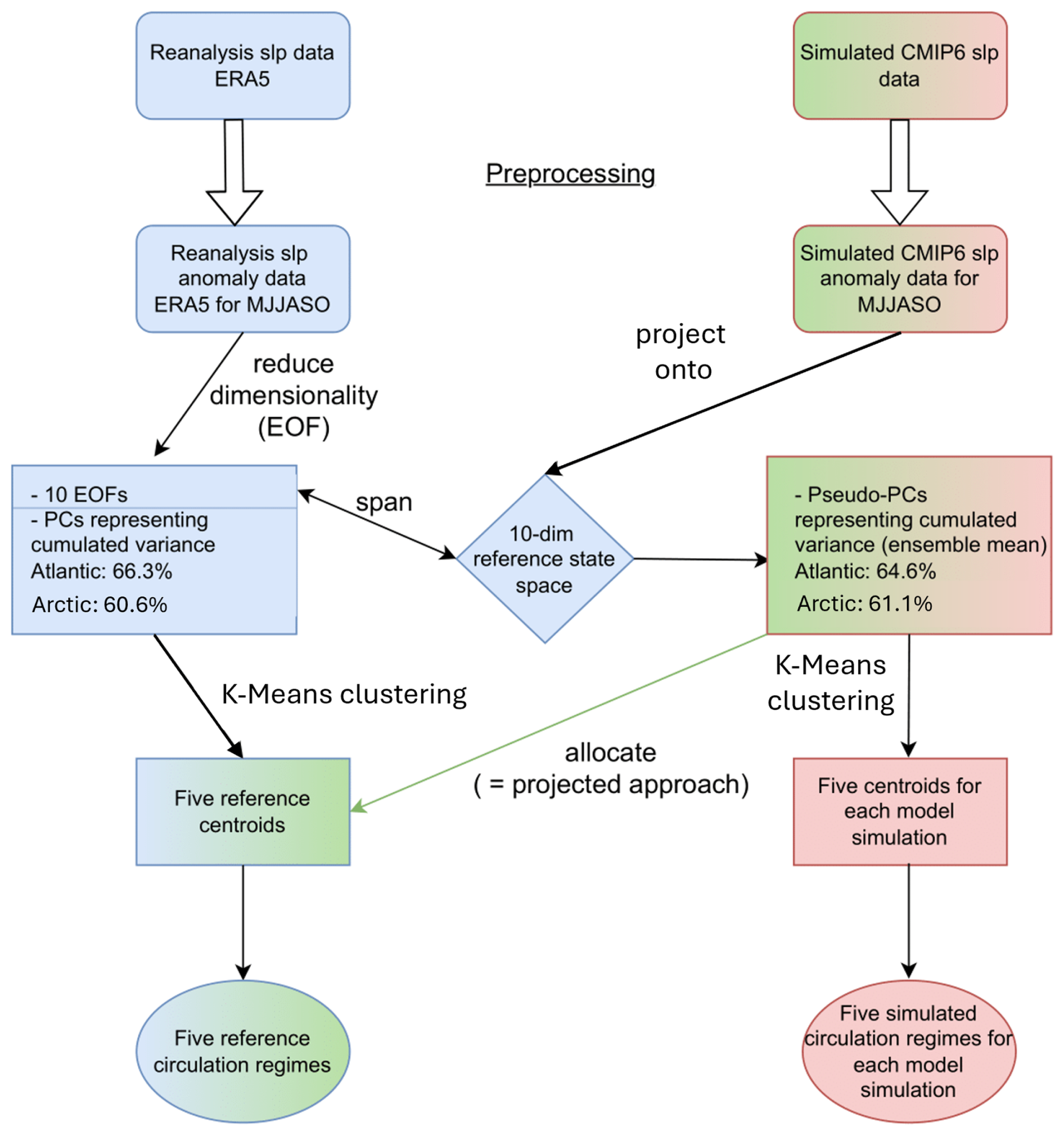
Figure 1 Chart flow of computation of atmospheric circulation regimes. The blue pathway indicates the approach to calculate reference circulation regimes. The red pathway shows the procedure to calculate simulated circulation regimes, the green pathway represents the projected regimes.

To obtain reference atmospheric circulation regimes, a K-Means clustering algorithm is applied in the ten-dimensional reduced state space. The PCs serve as the input data for the clustering algorithm. Each data point is assigned to its cluster centre, or centroid, which is selected to maximize inter-cluster distance while minimizing intra-cluster distance. In the case of the climate model data (red pathway in Fig. 1), the SLP anomalies are not reduced in their dimensionality via an EOF analysis. As in Fabiano et al. (e.g. 2020, 2021) an alternative approach was taken, whereby the anomalies were projected onto the ten-dimensional reference state space. This results in the generation of pseudo-PCs. The pseudo-PCs afterward are clustered via the K-Means clustering algorithm to obtain simulated circulation regimes for each model simulation in both time periods that differ in their spatial structure compared to the reference circulation regimes. Projecting the CMIP6 model data onto the ERA5 reference state space ensures that all calculations are performed in the same reference space, enabling consistent comparison of regime patterns. Nonetheless, the pseudo-PCs describe less variance than the models own PCs and this might introduce biases in our analysis. Following Fabiano et al. (2020), we tested the consistency between clustering in the pseudo PC-space versus clustering in the models' own PC-space by analysing the variance ratio, i.e. the ratio between the mean inter-cluster squared distance and the mean intra-cluster variance for K-Means clustering in the pseudo PC-space versus clustering in the models' own PC-space for the common model clusters over the North-Atlantic–Eurasian region for the present-day period. We also compared these results with the variance ratio for the ERA5 reference clusters (see Appendix A). The model simulations have a lower variance ratio than the ERA5 data and are outside the ERA5 variability range. The variance ratio revealed a slight increase in the Pseudo-PC space, indicating stronger clustered data. Nonetheless, the difference to the variance ratio in the models own PC-space is not significant and the variability range is similar. In addition, we investigated whether the cluster centers obtained with both approaches represent the same patterns (Appendix A) and found very similar patterns with pattern correlations higher than 0.95. Both the analysis of the variance ratio and the evaluation of the cluster center patterns support the applicability of the projected approach for our analysis.

The projected approach (green pathway in Fig. 1) allocates the pseudo-PCs directly to the reference centroids, by finding their closest reference centroids (in terms of Euclidean distance) from the ERA5 reanalysis. In other words, we assign the data from the CMIP models to the regimes from ERA5 by using the pseudo-PCs. This assignment of each day to the ERA5 reference clusters has been calculated for historical and future time periods. In order to provide a joint representation of the climate models' circulation regimes, the common simulated circulation regime framework is applied, which will be used to represent the characteristic joint regimes for the entire model ensemble. The common simulated circulation regime framework enables the possibility to compare the spatial structure between reanalysis and the entire ensemble of CMIP6 models. First the preprocessed data of each climate model are merged into a single data file along the temporal axis, either for the historical period 1985–2014 or the future period 2070–2099. Instead of performing a common EOF analysis to derive shared principal components (as described, for example, in Benestad et al., 2023), the common climate model data are projected onto the ten-dimensional reference state space defined from the ERA5 data. This projection yields ten common pseudo-principal components (Pseudo-PCs). The common Pseudo-PCs serve as input data for the K-Means clustering algorithm that is applied. Five common simulated circulation regimes are obtained for each time period, representing the joint regimes for the entire model ensemble.

3.2.2 SANDRA

In order to investigate the sensitivity of the results to the choice of clustering method, a second method was also applied. Simulated annealing and diversified randomisation clustering (SANDRA, Philipp et al., 2007) differs from K-means clustering by introducing a randomised cluster assignment inspired by the thermally induced movement of atoms in a crystal lattice (hence the term “annealing”, from the process in metallurgy). A cooldown factor is used to gradually decrease the movements, resulting in a positioning which is numerically very efficient at finding solutions close to the global optimum. Details are found in Philipp et al. (2007). The application in the present study is based on the implementation in the cost733class software (Philipp et al., 2016). Comparisons of SANDRA with other methods show very favourable results (Røste and Landgren, 2022; Tveito and Huth, 2016).

In contrast to the K-Means clustering algorithm, we only followed the projected approach for SANDRA, i.e. the SANDRA algorithm was trained on the ERA5 reanalysis data and then the resulting five regimes were assigned to all climate models, for both the historical and future periods. The SANDRA method was applied for both the 1.125° horizontal resolution used in KME method as well as a coarser 2.5° resolution. Unsurprisingly, the resulting regimes were almost identical (with spatial correlation > 0.998 for all 5 patterns, and maximum absolute difference below 0.5 hPa, not shown), and we decided to use the coarser resolution for computational efficiency.

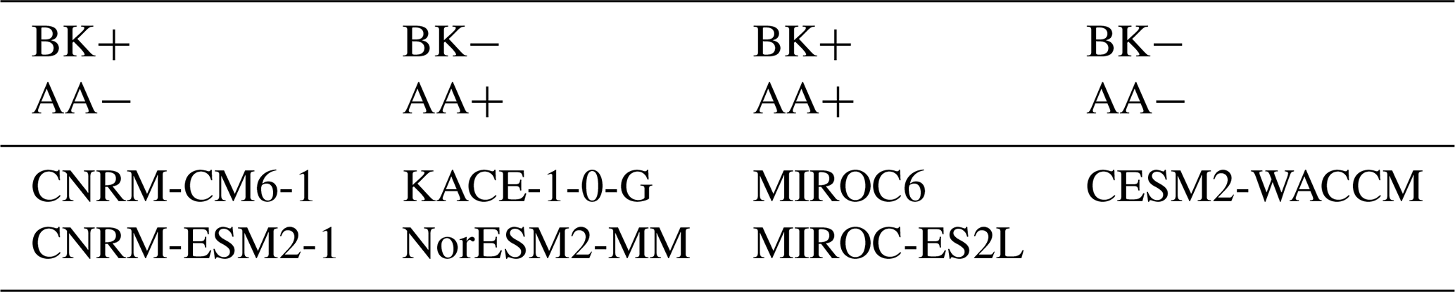
Table 1 Storyline and respective model selection. The predictors are accompanied with ± representing a strong/weak Barents–Kara Sea Warming or Arctic Amplification.

3.2.3 Determining the Number of Clusters

In almost all clustering algorithms, the number of clusters must be predetermined, and this is a topic of extensive discussion in the literature, as referenced in the following sources: Stephenson et al. (2004); Madonna et al. (2017); Straus et al. (2007); Falkena et al. (2020). Several methods have been applied to determine an optimal number of regimes, with most studies indicating a number of regimes between four and six for North-Atlantic winter regimes (Falkena et al., 2020). Here, we have based the decision for a reasonable number of circulation regimes on three metrics described in detail in the Appendix C: The anomaly correlation coefficient between the patterns of the clusters, following Grams et al. (2017) have been applied for both methods, K-Means and SAN. In addition, the elbow test and the silhouette score have been applied for K-Means. The elbow test assesses the efficiency of allocation of centroids (Olmo et al., 2024) and the silhouette score measures the quality of clustering (Rousseeuw, 1987). All three metrics support a choice of k = 5 clusters for both regions. This is also in agreement with cluster numbers used in other studies for winter North-Atlantic regimes, e.g. in Crasemann et al. (2017).

3.2.4 Statistical Evaluation Methods

The performance of models in reproducing the spatial structure of reference circulation regimes is evaluated using a Taylor diagram (Taylor, 2001). This method incorporates two statistical measures: the spatial correlation coefficient (R) between simulated and reference regimes, and the normalized standard deviation (SD) of anomalies. These metrics are plotted on a polar diagram, where the angular axis represents R, the radial axis indicates SD. The Taylor diagram provides a compact visualization of model performance, aiding in the comparison of spatial structures.

To determine statistical significance of the changes in frequency of occurrence under the influence of rising GHG emission in the future for both regions, Welch's t-test is employed (Welch, 1947). Welch's t-test is a robust tool for comparing group means, and is particularly effective when variances are unequal. Here we use it to evaluate whether observed differences in the frequency of circulation regimes are statistically significant compared to historical records, providing insights into potential climate-related anomalies in future projections.

3.3 Storylines

In the context of climate research, the term “storyline” is used to group together climate models that exhibit a certain physically consistent response in their future climate change (Trenberth et al., 2015; Shepherd, 2016; Shepherd et al., 2018). This approach emphasizes an understanding of the driving factors behind climate events and their plausibility, without the assignment of a priori probabilities. The use of multiple storylines allows for the exploration of a range of potential futures. This approach raises risk awareness by framing risks in an event-oriented manner, which aligns with how people perceive risk. Additionally, it strengthens decision-making by integrating climate change information with other factors to address compound risks. As argued in Levine et al. (2024), a considerable proportion of the variability in the surface climate response to global warming in the Arctic during the extended summer season is linked to two predictors; the warming of the Barents–Kara Sea (BK) and the Arctic lower troposphere (Arctic Amplification, AA). We consider all four storylines for a comprehensive analysis. Following the results from Levine et al. (2024), these storylines can be most closely represented by the CMIP6 models presented in Table 1.

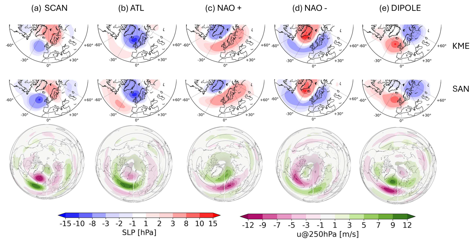
Figure 2 Reference circulation regimes for the North Atlantic–Eurasian region in the extended summer season, May to October, in the historical time period (1985–2014) from the ERA5 dataset, calculated by the K-Means (KME) and SANDRA (SAN) algorithms. In the lower row the zonal wind anomaly composites for KME regimes at 250 hPa are shown, the SAN wind composites indicate similar anomalies (Appendix Fig. F1).

4 Results

4.1 North Atlantic–Eurasian Region

4.1.1 Spatial regime patterns for the present day

Five atmospheric circulation regimes are detected in the North Atlantic–Eurasian region. The reference circulation regimes for the ERA5 data 1985–2014 obtained with the K-Means clustering (KME, Fig. 2, upper row) and the SANDRA (SAN, Fig. 2,center row) algorithm alongside with the zonal wind anomaly composites at 250 hPa for the KME regimes, lower row, are summarised here, the wind composites linked to the SAN regimes are shown in Appendix F.

• The Scandinavian Blocking regime (SCAN), shown in Fig. 2a, indicates a positive pressure anomaly centered above Scandinavia and a low pressure anomaly, centered over the North Atlantic Ocean westwards of the British Isles (refer to KME, Fig. 2a, upper row). The regime pattern obtained by the SAN algorithm displays a slightly weaker positive pressure anomaly over Scandinavia and a slightly stronger low pressure anomaly over the North Atlantic (Fig. 2a, center row). The SCAN is associated with a southward shifted Atlantic jet.

• The Atlantic Trough regime (ATL) is characterized by a strong negative pressure anomaly centered between Iceland and the British Isles (Fig. 2b), connected with a strengthening of the Atlantic jet exit.

• Figure 2c displays the North Atlantic Oscillation, which is poleward shifted in summer, in its positive phase (NAO+). Here an elongated positive pressure anomaly extends from the Ural to Newfoundland accompanied by a negative pressure anomaly above Greenland. The NAO+ pattern is connected with a poleward shifted and slightly tilted Atlantic jet.

• Figure 2d displays the North Atlantic Oscillation in its negative phase (NAO−), here the positive and negative pressure anomalies are swapped, respectively to NAO+ as well as the wind anomalies, which indicate a southward shifted Atlantic jet.

• The Dipole Atlantic Blocking regime (DIPOLE, Fig. 2e) displays a positive pressure anomaly centered between Iceland and the British Isles. The accompanying negative pressure anomaly is located over the Ural region and the Barents Sea. The DIPOLE pattern is linked to a weakening of the Atlantic jet exit and poleward shift of the jet structure.

Riebold (2023) analysed circulation regimes over the same region for the summer season June to August (JJA) and found similar MSLP anomaly patterns for each regime. Boé et al. (2009) and Cattiaux et al. (2013), on the other hand, analysed summer circulation regimes for JJA over a smaller North Atlantic region (20–80° N, 90° W–30° E), using SLP (Boé et al., 2009) and Z500 (Cattiaux et al., 2013) data, respectively. In both studies, four circulation regimes were detected. These four regimes comprise the negative and positive phases of the NAO (called NAO− and Blocking, BL), an Atlantic low (AL) and an Atlantic ridge (AR) regime, which bear many similarities with the NAO−, NAO+, ATL and SCAN regimes detected in our study.

The agreement between the characteristic regime patterns of both algorithms, KME and SAN, is evaluated by means of a Taylor plot in Fig. 3, where the KME patterns serve as reference. The correlation coefficient for all clusters are above 0.85 and the spatial standard deviation of the patterns obtained with the SAN method are close to the reference values. Two patterns, ATL and NAO−, exhibit even very high spatial correlation values above 0.95. The spatial similarity between the clusters calculated from KME and SAN algorithm is validated by these findings.

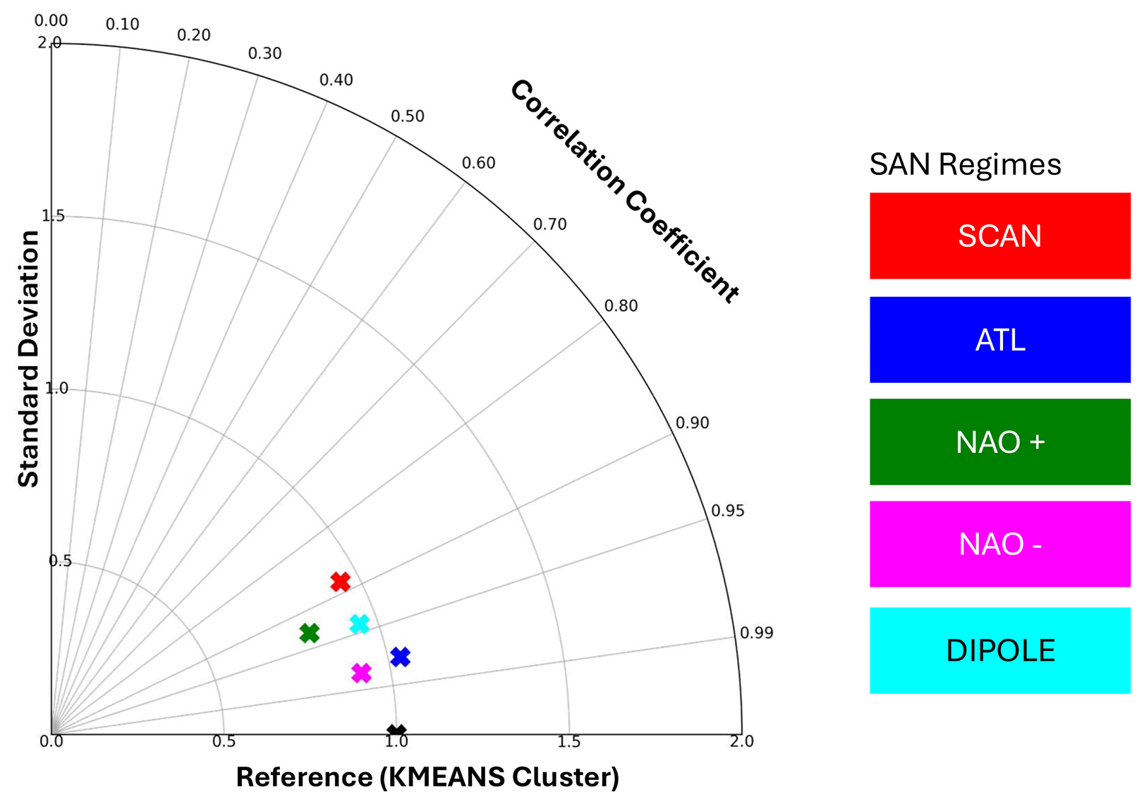
Figure 3 Taylor diagram analysis of circulation regimes computed by KME and SAN algorithms in the historical period for the North Atlantic–Eurasian region in extended boreal summer season from May to October. The reference circulation regimes computed from ERA5 reanalysis data with KME is marked as black cross, the colored crosses represent the SAN regimes.

4.1.2 Future changes for the North-Atlantic regimes

In Sect. 3.2.1 two different methods to calculate circulation regimes for the model simulations were presented: the projected approach and the simulation circulation regime approach. The simulated common circulation regimes for the extended boreal summer season for the future period, revealing the joint regimes for the whole ensemble of climate models, exhibit small differences in their spatial structure compared to the reference circulation regimes computed from reanalysis ERA5 data. The evaluation by means of a Taylor plot is presented in Fig. 4 for the North Atlantic–Eurasian region. The calculated common simulated circulation regimes in the future period exhibit high spatial correlation coefficients with the ERA5 reference circulation regimes. The correlation coefficients reach values above 0.85 for KME regimes and above 0.7 for SAN patterns and the standard deviations of the common simulated circulation regimes are found to be between 0.8 and 1.4 compared to the normalized reference standard deviation of 1.

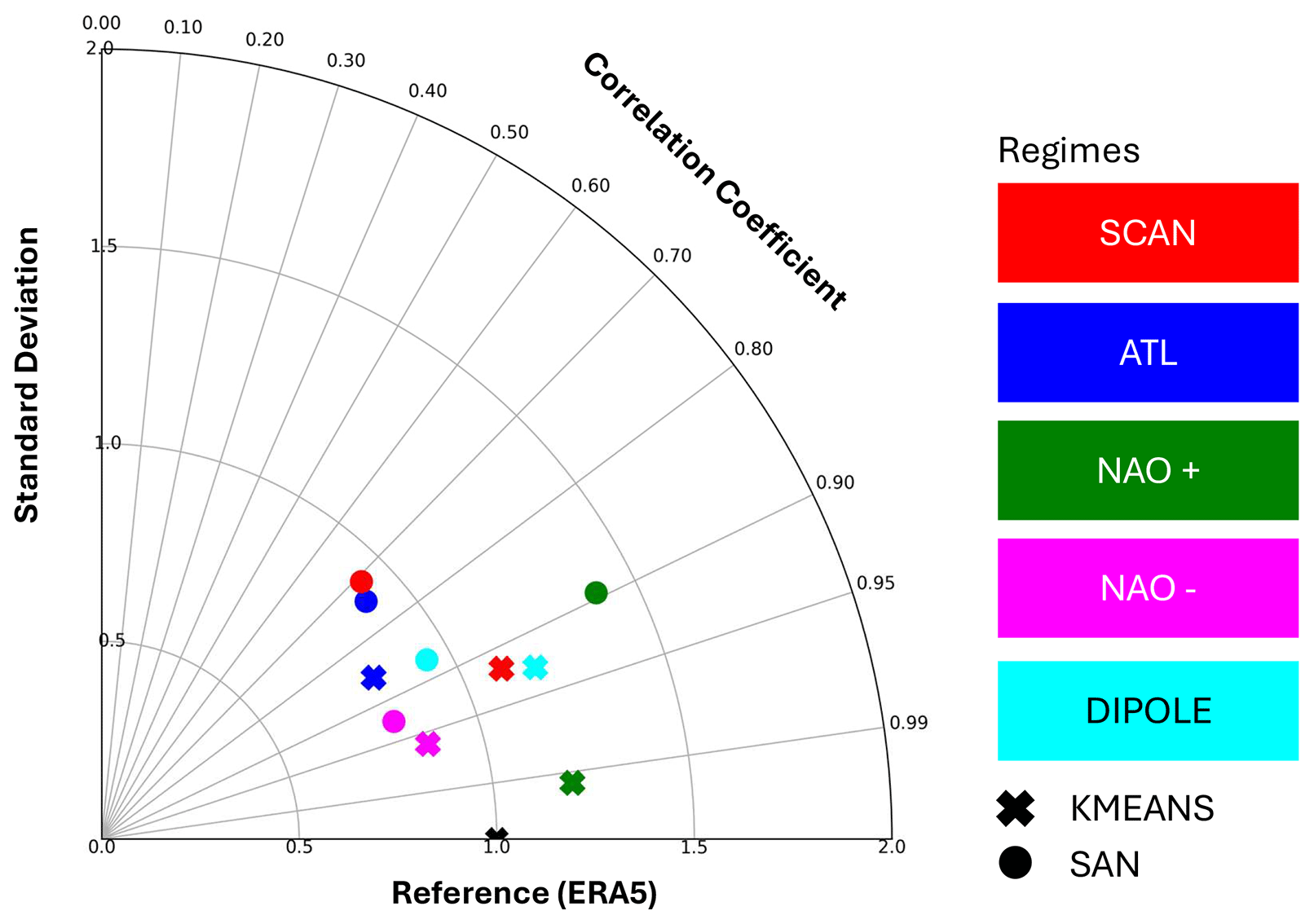
Figure 4 Taylor diagram comparing the future common simulated regimes for the CMIP6 ensemble for SSP5-8.5 and the period 2070–2099 to the corresponding reference regimes from ERA5 reanalysis in the historical period (1985–2014), for the North Atlantic–Eurasian region. Spatial regime patterns determined with K-Means clustering represented as crosses. SAN patterns are indicated by circles.

These results support the hypothesis of Palmer (1993) and Corti et al. (1999) introduced in Section 1, namely that a rather weak external forcing acting on the dynamical system atmosphere does not alter the spatial structure of the regime patterns. In our case, even under the high emission scenario SSP5-8.5 the spatial structure remains largely unchanged in the future time period.

This allows us to apply the projected approach for the calculation of the frequency of regime occurrence for the climate models in the historical and future period. Additionally, the projected approach is able to calculate the frequency of occurrence of the circulation regimes of the CMIP6 models more accurately than the simulated circulation regime approach. This is visualised in Fig. 5 for both regions, the absolute difference between the simulated respective projected and reference circulation regimes frequencies averaged over all regimes for each model in the historical period, i.e. the frequency bias as defined in Fabiano et al. (2021) is shown. The mean frequency bias is smaller for the projected circulation regimes compared to the simulated circulation regimes. The interquartile range of the projected circulation regimes' frequency bias is lower compared to the interquartile range of the simulated circulation regimes' frequency bias. Fabiano et al. (2021) suggested that a lower frequency bias results in a higher confidence to project changes in the frequency of occurrence under climate change. Due to this, the projected approach is preferable in the analysis of changes in the frequency of occurrence for both regions.

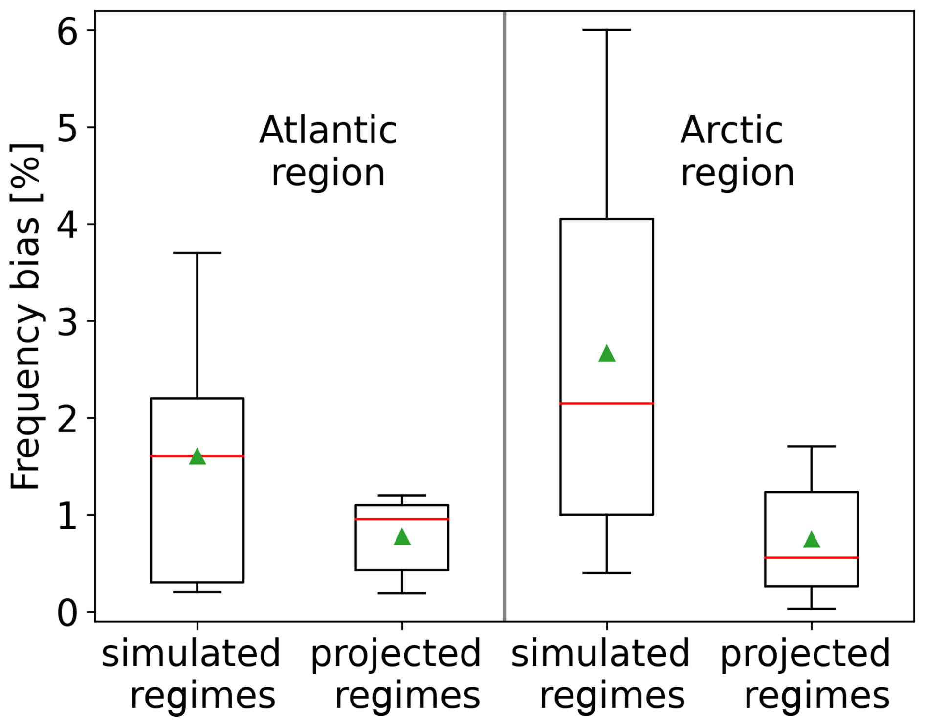
Figure 5 Box plot of frequency biases for North Atlantic–Eurasian and Arctic region of simulated (respective projected) circulation regimes compared to the reference circulation regimes in the historical period. The median is shown as a red line, the mean is indicated as a green triangle. The boxes represent the first and third quartiles, the top and bottom bars denote the 10th and 90th percentiles.

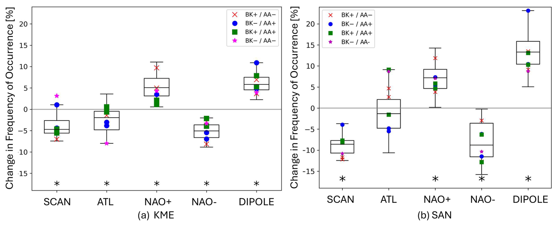
Figure 6 Changes in the frequency of occurrence for the North Atlantic–Eurasian region under global warming (SSP5-8.5 scenario) compared to the historical period, in the extended boreal summer season May to October. The boxes denote the first and third quartiles, the center black line indicates the ensemble median and the top and bottom whiskers represent the 10th and 90th percentiles. Stars indicate significant changes compared to the historical data at the 95 % confidence level calculated with Welch's t-test. The markers represent models attributed to the respective storylines.

We now turn to analyse the projected future changes under the SSP5-8.5 scenario. The changes in the frequency of occurrence for circulation regimes computed by both methods, KME and SAN, are shown in Fig. 6. The change in the frequency of occurrence for a pattern is the difference between the percentage of days assigned to that particular pattern in the future (2070–2099) and in the historical time period (1985–2014) in the extended boreal summer season from May to October. This is calculated for each of the twenty CMIP6 models, with the spread of the models visualised in the box plot. Both methods show consistent results for all five clusters, only the SAN method indicate non-significant results for the ATL pattern. Regarding the SCAN pattern, both methods detected a decrease in the frequency of occurrence in the future for most of the models. Here models linked to BK+/AA− storylines exhibit a stronger decrease in their frequency of occurrence in the future. In contrast, the BK−/AA+ linked models exhibit only small changes, even a positive change in the frequency for KME method, BK+/AA+ associated models are in close proximity to the model mean. For the ATL pattern, both methods show a decrease in its frequency of occurence under strong global warming, only significant for the KME algorithm. Models connected with the BK−/AA+ storylines show rather stronger decreases in their frequency of occurrence under global warming. For both methods, i.e. SAN and KME, the NAO+ pattern occurs significantly more frequent in the future period compared to the historical period under the GHG forcing projected by the SSP5-8.5 scenario. The NAO+ pattern is linked to a tilted, polewards shifted Atlantic jet structure, thus this results suggests the jet will be shifted northwards under strong global warming in the season from May to October, which is concurrent with the changes from June to August found in Simpson et al. (2014) and the annual mean in Stendel et al. (2021). The NAO− pattern displays a significant decrease in occurrence frequency in the future, as detected with both algorithms. As the NAO− pattern is associated with a southward shifted Atlantic jet, this decrease in frequency of occurrence underlines the suggestion made analysing the NAO+ pattern, i.e. the Atlantic jet will be shifted northwards. In Boé et al. (2009), who analysed a more confined region in the summer season utilising CMIP3 climate models, an increase in NAO+ and decrease in NAO− was also found, which is in line with the presented findings. For the DIPOLE pattern, both methods show a significant increase in their frequency of occurrence, that is stronger when applying the SAN method. Likewise to the NAO+ pattern, the DIPOLE regime is linked to the northward shifted jet structure and shows a positive change in its frequency of occurrence under global warming.

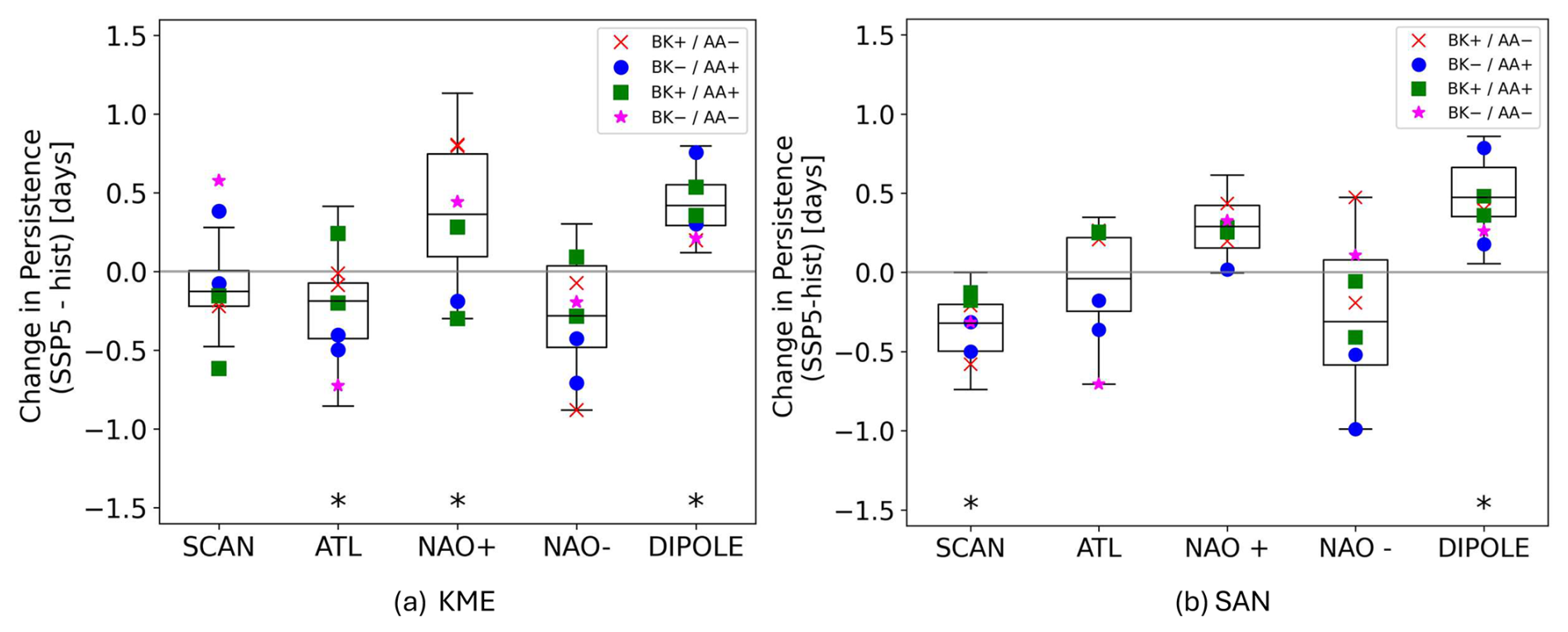
Figure 7 Changes in persistence for the North Atlantic–Eurasian region under global warming (SSP5-8.5 scenario) compared to the historical period, in the extended boreal summer season May to October. The boxes denote the first and third quartiles, the center black line indicates the ensemble median and the top and bottom whiskers represent the 10th and 90th percentiles. Stars indicate significant changes compared to the historical data at the 95 % confidence level calculated with Welch's t-test. The markers represent models attributed to the respective storylines.

The changes in frequency of occurrence may arise from two different sources: change in how often events occur or for how long they persist. The latter is analysed in the following for the North Atlantic–Eurasian region, shown in Fig. 7. The analysis reveals that changes in persistence largely mirror those in the frequency of occurrence. For the KME method, the significant shifts identified in occurrence frequency are likewise evident in persistence, with the exception of the SCAN and NAO− regimes, whose persistence change is not statistically significant yet follows the same directional trend, suggesting that the future changes are due to the regimes becoming less persistent as well as occurring less often in the future. For the SAN algorithm, the significant alterations in frequency of occurrence for SCAN and DIPOLE are also reflected in persistence. By contrast NAO+ and NAO− do not exhibit a corresponding significant change, meaning the change in frequency of occurrence for the NAO patterns may be due to both: a change in persistence of the regimes as well as the events occurring more/less often in general. For both algorithms, as well as for both metrics, i.e. frequency of occurrence and persistence, the BK−/AA+ storyline for the ATL regime display a more robust negative trend. All other regimes do not show any dependence of the changes in occurrence frequency on the storyline. One reason for that might be the small sample size of only one or two models representing each storyline.

To summarise, both methods, the KME and SAN calculate typical circulation regimes for the North Atlantic–Eurasian region, which are similar in their spatial structure. The simulated changes in the spatial structure due to the influence of climate change in the atmosphere are small for the whole ensemble of climate models, but the frequency of occurrence is altered as suggested by Corti et al. (1999), see also the Introduction (Sect. 1). Both methods detect a significant increase in the occurrence of the NAO+ and DIPOLE pattern in the future under strong GHG forcing, the change of the SAN method is higher in its median and interquartile range. The same applies for the future change of the NAO− regime, both methods simulate a significant decrease in their frequency of occurrence. Most of the results are in line with the findings regarding the persistence. Overall we found a high correspondence between future changes in occurrence and persistence. The analyses of the related zonal wind composites revealed that regimes associated with a northward shifted jet stream are simulated to occur more often and to be more persistent, while patterns linked to a southward shifted jet stream occur less often under strong global warming.

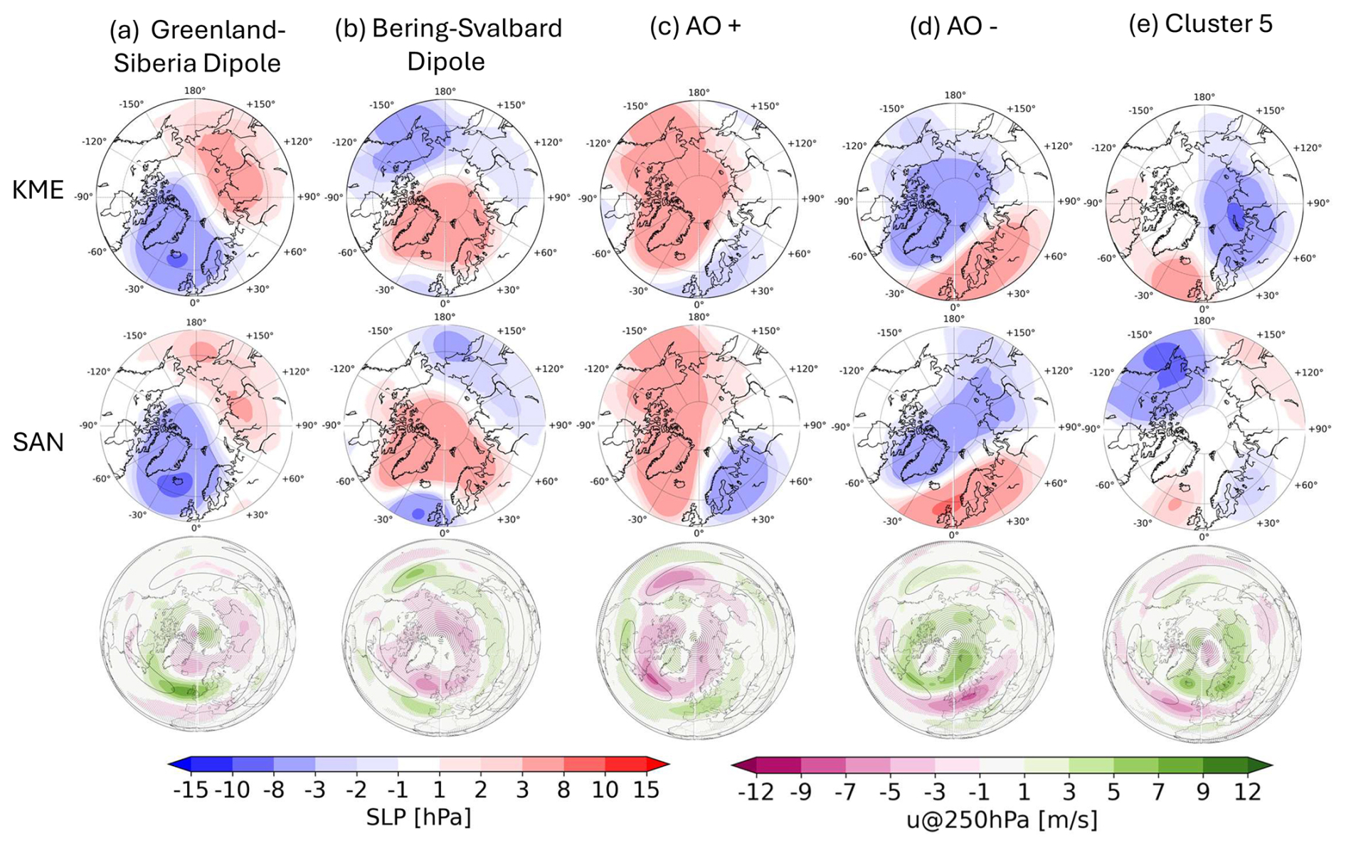
Figure 8 Reference circulation regimes for the Arctic region in the historical time period (1985–2014) from the ERA5 reanalysis dataset, calculated by the K-Means Clustering (KME) and simulated annealing and diversified randomisation clustering (SAN) algorithms. In the lower row the zonal wind anomaly composites for KME regimes at 250 hPa are shown, the SAN wind composites indicate similar anomalies except for Cluster 5.

4.2 Arctic Region

4.2.1 Spatial regime patterns for the present day

For the Arctic region, five atmospheric circulation regimes are determined based on the arguments in Sect. 3.2.1. The reference patterns calculated by both methods, KME and SAN, for the ERA5 data are shown in Fig. 8, upper two rows. Additionally, the zonal wind anomaly composites for KME regimes at 250 hPa are shown in the lower row. The zonal wind anomaly composites respective to the SAN regimes are shown in Appendix F.

• Greenland-Siberia Dipole(Fig. 8a) is characterized by a negative pressure anomaly above Iceland and Greenland facing a positive pressure anomaly above Siberia resulting in a strong westerly flow across the Arctic region. The zonal wind composites at 250 hPa show a strengthening of the Atlantic jet exit.

• Bering–Svalbard Dipole (Fig. 8b) is characterized by a positive pressure anomaly centered above Greenland and extending towards the Barents Sea and a negative pressure anomaly centered at Kamchatka. The Bering–Svalbard-Dipole is associated with a southward shifted Atlantic jet and strengthening of the Pacific jet exit.

• Arctic Ocean High (AO+, Fig. 8c) is a (strong) positive pressure anomaly above the Arctic Ocean. The wind composite show a southward shifted Atlantic jet and weakening of the Pacific jet.

• Arctic Ocean Low (AO−, Fig. 8d) displays a (strong) negative pressure anomaly is centered above the Arctic. Note that AO+ and AO− have very similar patterns but with opposite sign. In contrast to the AO+ pattern, the AO− shows a poleward shifted Atlantic jet and slight strengthening of the Pacific jet.

• Cluster 5 (Fig. 8e) shows a negative pressure anomaly above the Barents Sea which extends to the Laptev Sea when using the KME method. A positive pressure anomaly is also found in the pattern calculated by the SAN algorithm opposing the negative pressure anomaly. For the KME method, the positive pressure anomaly is above the North Atlantic Sea. Here the wind composites show different shifts regarding the regimes computed by KME and SAN algorithm. The KME wind composites indicates a poleward shifted Atlantic jet. The SAN regime is associated with a strengthening of the Pacific jet exit and is shown in Appendix F

From visual inspection of Fig. 8, it is clear that the two methods agree quite well on the first four patterns, while Cluster 5 is more different. We note that the low pressure in the Bering–Svalbard Dipole cluster is located over Alaska in KME, while it is more towards Kamchatka in SAN. This is compensated in SAN by grouping together days with low pressure over Alaska in Cluster 5 (Of the days that are assigned to the Bering–Svalbard KME pattern only 48.8 % is assigned to the Bering–Svalbard SAN pattern, while 35.1 % is assigned to Cluster 5 SAN underlining the spatial similarity between the two patterns).

Similar to the North Atlantic–Eurasian region, the spatial patterns obtained by both methods are compared by a Taylor plot in Fig. 9, where the patterns calculated by the KME algorithm serve as reference. The regimes show correlation coefficients between 0.78 and 0.95, thus the spatial structure of every pattern is similar for both methods, KME and SAN, except for Cluster 5. The standard deviations of the magnitudes of the SLP anomalies are close to the reference for all five patterns, slightly under the normalized value of one for Cluster5, AO+ and AO−. To conclude, both methods, KME and SAN, calculate four clusters with similar spatial structure for the Arctic region in the extended boreal summer season May to October in the historical time period 1985–2014 from ERA5 reanalysis data, but the 5th cluster shows substantial differences.

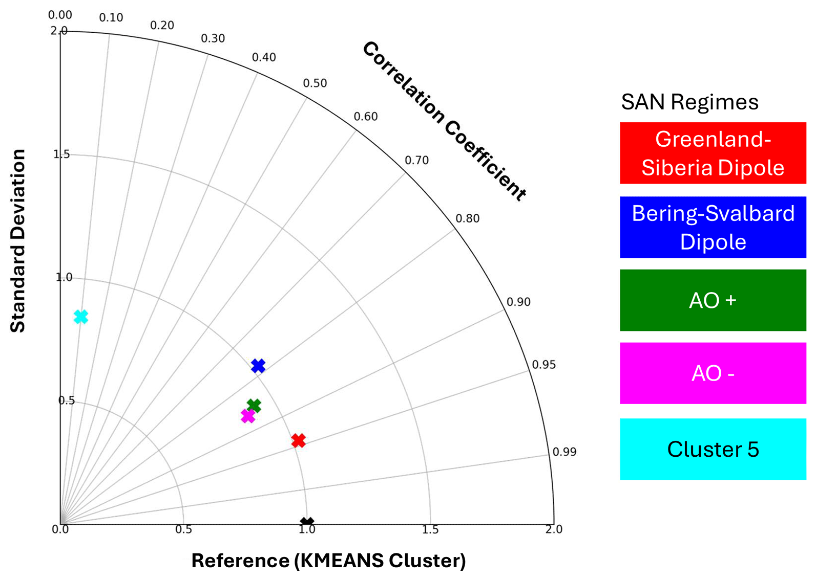
Figure 9 Taylor diagram analysis of circulation regimes computed by KME and SAN algorithms in the historical period for the Arctic region in extended boreal summer season from May to October. The reference circulation regimes computed from ERA5 reanalysis data with KME is marked as black cross. The colored crosses represent the respective regime calculated from SAN algorithm.

4.2.2 Future changes for the Arctic circulation regimes

In Fig. 10 the Taylor diagram comparing the circulation regime structure changes under the strong SSP5-8.5 scenario compared to the reference historical ERA5 regimes for KME and SAN algorithm is shown. The standard deviations differ from the reference (normalized to 1), more pronounced for the SAN algorithm, as the standard deviation for the Bering–Svalbard Dipole is 0.57 and for Cluster 5 above 1.5, indicating a change in the magnitudes of the pressure anomalies. However, the correlation coefficient remains above 0.7 for all patterns across both algorithms. Alongside with the arguments in Sect. 4.1 and Appendix A, the projected approach is applied to analyse changes in regime occurrence frequencies between the historical and future periods for the Arctic region. These results are shown in Fig. 11 for both methods, KME and SAN. The future frequency of occurrence of the Greenland–Siberia Dipole shows no consistent change in both methods, as the SAN regime is simulated to occur more often and the KME regime less often in the ensemble median. For the regimes calculated by the KME algorithm, the AO+ regime occurs less frequently in the future which is in agreement with the results obtained by the SAN algorithm. The AO− regime occurs significantly more often in the future time period for both methods. Cluster 5 shows a significant positive change in its frequency of occurrence for the KME algorithm and a strong negative trend regarding the SAN method. This finding underlines the assumption that the SAN Cluster 5 is compensating the shifted low pressure anomaly above Kamchatka in the Bering–Svalbard Dipole present in the KME method. A decrease in the frequency of low pressure events in this area therefore shows up as a negative frequency change in Bering–Svalbard dipole for KME but Cluster 5 in SAN. Additionally, the KME Bering–Svalbard Dipole and SAN Cluster 5 are both linked to a stengthening in the Pacific jet. Similar to the North Atlantic–Eurasian region, the interquartile range of the frequency changes for the SAN regimes is greater compared to the KME regimes, especially regarding the Bering–Svalbard Dipole and AO−.

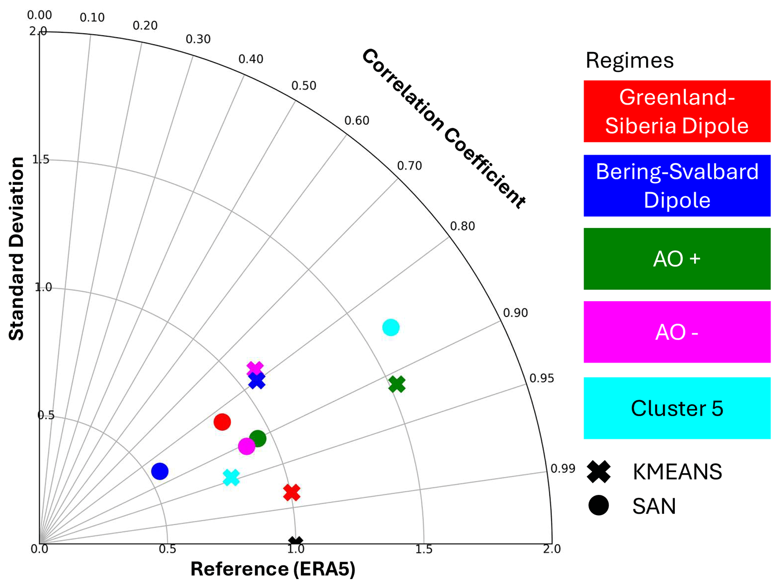
Figure 10 Taylor diagram comparing the future common simulated regimes for the CMIP6 ensemble for SSP5-8.5 and the period 2070–2099 to the corresponding reference regimes from ERA5 reanalysis in the historical period (1985–2014), for the Arctic region. Spatial regime patterns determined with K-Means clustering are represented as crosses. SANDRA patterns are shown as circles.

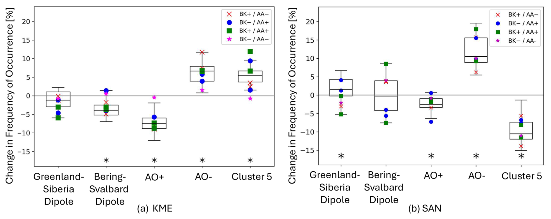
Figure 11 Changes in the frequency of occurrence for the Arctic region under global warming compared to the historical period, SSP5-8.5 scenario in the extended summer season May to October. The boxes denote the first and third quartiles, the center black line indicated the ensemble median and the top and bottom whiskers represent the 10th and 90th percentiles. The star indicated a significant changes compared to the historical data at the 95 % confidence level calculated with Welch's t-test. The markers represent models attributed to the respective storylines

The following statements can be made when comparing the results for Arctic and North Atlantic–Eurasian region: Considering the spatial patterns shown in Fig. 8, the circulation regime characterized by a negative pressure anomaly above the Arctic center; AO− is simulated to occur more frequently in the future period for both investigated algorithms. This change is consistent with the increase in the frequency of occurrence of the NAO+ regime found in the North Atlantic–Eurasian region in the future time period, since both patterns, AO− and NAO+ exhibit spatial similarities, i.e. a negative pressure pressure anomaly above Greenland and a broad positive pressure anomaly above Northern Europe (see Figs. 2c and 8d). Both patterns are linked to a northward shifted Atlantic jet, and projected to occur more often in the future. The circulation regimes associated with positive pressure anomalies above the Arctic; Bering–Svalbard Dipole and AO+ are expected to occur less frequently in the future. Again, AO+ and NAO− (from the analysis over the North Atlantic–Eurasian region) are both characterized by a positive pressure anomaly above Greenland and a negative pressure anomaly extending from the Ural to the North Atlantic. The AO+ regime is connected with a southward shifted jet structure above the Atlantic, likewise to the NAO− regime, supporting the findings in the North Atlantic–Eurasian region.

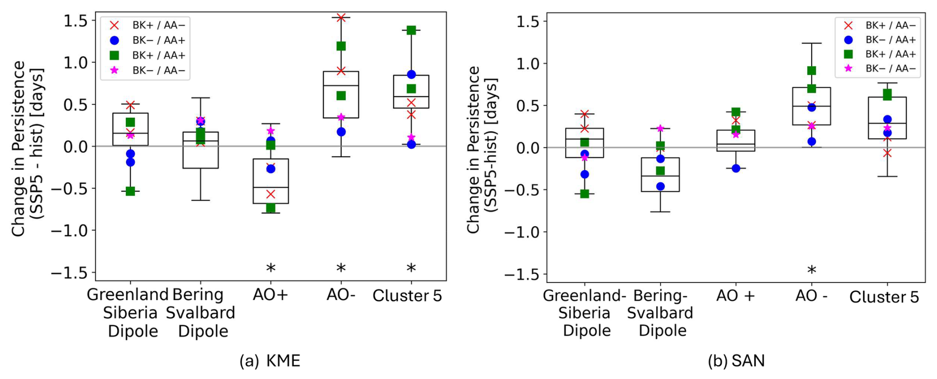
Figure 12 Changes in persistence for the Arctic region under global warming compared to the historical period, SSP5-8.5 scenario in the extended summer season May to October. The boxes denote the first and third quartiles, the center black line indicated the ensemble median and the top and bottom whiskers represent the 10th and 90th percentiles. The star indicated a significant changes compared to the historical data at the 95 % confidence level calculated with Welch's t-test. The markers represent models attributed to the respective storylines.

Most of the found changes in frequency of occurrence can be also observed by analysing the change in persistence for the Arctic region (refer to Fig. 12), although the results are not as corresponding as for the North Atlantic–Eurasian region. The indicated change in persistence for the Greenland-Siberia Dipole for both methods is positive, which supports the trend for the frequency of occurrence for this pattern regarding the SAN method, although the change is not significant. For the Bering–Svalbard Dipole there are non-significant future changes in persistence that are inconsistent with the changes indicated in the frequency of occurrence, refer to Fig. 11, meaning the change in frequency of occurrence for the Bering–Svalbard Dipole may be due to the event occurring less often in the future rather than a decreasing persistence. Only for the KME method the changes in frequency of occurrence of the AO+ pattern are consistent with the future persistence changes, where the change in persistence is almost zero and non-significant. This finding indicates that the occurrence of shorter AO+ events may be more prevalent in the SAN method. The AO− shows more robust results, indicating a significant positive change in persistence for both methods. Here, the models linked to the BK+/AA+ storylines exhibit stronger signals compared to the opposing BK−/AA− storylines' models. Cluster 5 again shows a higher persistence that supports the findings from the frequency of occurrence for KME. In contrast for the SAN method, Cluster 5 is simulated to occur significantly less frequently in the future and the persistence even shows a slight longer persistence, indicating events to appear less often. The found results suggest that the correspondence between persistence and frequency of occurrence metrics is less robust in the Arctic compared to North Atlantic–Eurasian region.

As shown in Levine et al. (2024, Fig. 4), the CMIP6 multi-model mean (MMM) shows a poleward shifted Atlantic jet, but the strength of this poleward shift depends on the storyline, with a weaker poleward shift in storylines BK+/AA− and BK−/AA− and slightly stronger poleward shift in storylines BK+/AA+ and BK−/AA+ (compared to the MMM). The projected increase in the occurrence of NAO+, DIPOLE, and AO−, which are associated with a poleward shifted jet, supports this result. However, the specific changes in the storylines could not be attributed to shifts in occurrence frequency, likely due to the small sample size, as each storyline is based on only one or two CMIP6 models. To summarize, the calculated circulation regimes of both methods, KME and SAN, exhibit small changes under the influence of global warming in their spatial structure when analysing the Arctic region in the extended boreal summer season from May to October but the frequency of occurrence is changing significantly for most of the patterns. The simulated changes in the frequency of occurrence utilising the projected approach show a significant increase for the regime AO− for both methods. The changes in the frequency of occurrence are in line with the changes in persistence for this pattern, meaning the observed increasing the frequency of occurrence is due to longer lasting events. The AO+ pattern is projected to decrease significantly in frequency of occurrence under the influence of a strong GHG scenario in the future for both algorithms. In the Arctic region, the changes in frequency and persistence showed less agreement between the two methods and across both metrics than in the North Atlantic–Eurasian region. In contrast to the North Atlantic–Eurasian domain, where we detected a correspondence between occurrence and persistence changes for all regimes, in the Arctic region this correspondence is only found for the AO− regime.

5 Discussion and Outlook

This study investigates the impact of climate change on atmospheric circulation regimes in the North Atlantic–Eurasian and Arctic regions, focusing on their spatial structure, frequency of occurrence, and the respective changes along four specific storylines of summer Arctic climate change. Clustering algorithms (SAN and KME) and statistical analyses were used to assess the robustness of regime changes under the projected climate scenario SSP5-8.5.

The spatial structure analysis revealed consistent patterns between SAN and KME algorithms, identifying similar but not identical circulation regimes, with differences most pronounced in the Arctic domain over Kamchatka and Alaska, suggesting that these regions are more sensitive to methodological differences and results therefore less robust there.

The frequency of occurrence analysis has highlighted agreement between the two methods, with the results obtained by the SAN method showing a slightly stronger response and larger spread across the ensemble of CMIP6 models to future projections. In the North Atlantic–Eurasian region, the consistent increase in the positive North Atlantic Oscillation (NAO+) regime aligns with existing literature. For the Arctic, where regime analyses are sparse, both algorithms projected consistent changes across the Arctic Oceans patterns, offering valuable insights into how the Arctic atmospheric circulation responds to climate change. These findings emphasize the importance of regional assessments to capture the unique responses of distinct geographical areas to global climate change.

The storyline analysis revealed limited influence of localized drivers, such as Barents–Kara warming and Arctic Amplification, on large-scale circulation regimes. This highlights the complexity of regional processes and the need for continued research into the interplay between local climatic factors and broader atmospheric patterns.

The questions posed in the introduction can be answered as follows:

• 1.

  What are the projected future changes with focus on frequency of occurrence and persistence in atmospheric circulation regimes under a strong future climate change scenario?

  Under the SSP5-8.5 scenario, significant changes are projected in the frequency of atmospheric circulation regimes. The frequency of the positive North Atlantic Oscillation (NAO+) is expected to increase, consistent with prior research. This applies also to the simulated frequency changes of the AO− Arctic pattern which has similar pressure anomaly characteristics compared to NAO+. In contrast, the opposing circulation regime, i.e. NAO− is consistently simulated to occur less often in both methods. For the Arctic region, patterns associated with a negative pressure anomaly above the Arctic center (AO−) are expected to increase in their occurrence. Patterns linked with a positive pressure anomaly (AO+, Bering–Svalbard Dipole) are simulated to decrease in their frequency of occurrence, that is in accordance with the multimodel-mean change in mean sea-level pressure in Appendix G1. The spatial structure of these regimes remains largely unchanged, supporting the concept of Corti et al. (1999), that suggests stability of spatial regime structure under a weak external forcing on a dynamical system. The analysis of changes in persistence together with the frequency of occurrence help provide more insight of changes in dynamics. There is a tendency for patterns that occur more frequently in the future to also become more persistent. The tendency is more pronounced in the North Atlantic–Eurasian region than in the Arctic. This means for the Arctic region that if a pattern increases in its frequency of occurrence, it is rather due to the event to occur more often, and vice versa for a decrease.

  The changes in frequency and persistence show that patterns, that are associated with a poleward shifted jet structure will be more prominent under global warming, while patterns linked to a southward shifted jet stream will occur less often and also be less persistent. This result is in agreement with Li et al. (2024); Osman et al. (2021), who likewise identify northward-displaced Atlantic jet structures linked to global warming. Similar trends have previously been reported in CMIP3 (Woollings and Blackburn, 2012) and CMIP5 (Barnes and Polvani, 2013) simulations under strong global warming scenarios. The changes in the extended summer season from May to October are also in line with the northward-shifted Atlantic jet structure found in Simpson et al. (2014) for summer (June to August) and autumn (September to November).

• 2.

  How sensitive are the results to different methodological aspects (classification method, spatial domain)?

  The study employs two distinct clustering methods: K-Means (KME) and simulated annealing and diversified randomisation (SAN). The two methods produce nearly identical spatial structures of circulation regimes for the North Atlantic–Eurasian domain, but for the Arctic domain four of the five regimes are very similar while only the fifth differs considerably. While most spatial patterns are very similar, even small differences in the patterns can lead to differences in time-series assignments. This in turn leads to differences in the changes in frequency and persistence. Having two methods give similar results helps identify which circulation regimes and their associated future frequency and persistence changes are robust. For the North Atlantic–Eurasian region four out of five regimes show statistically significant future changes in frequency with same sign for both methods. For the Arctic domain, two out of five regimes show statistically significant future change with same sign for both methods. For persistence only one regime is statistically significant for both methods (holds true for both domains). While the North Atlantic–Eurasian domain has a generally prevailing westerly flow, the Arctic domain has a weaker and more variable circulation, especially during the summer season, which could contribute to a greater spread between the models, in turn giving less robust results for this domain.

• 3.

  How do the results in frequency of occurrence as well as persistence differ for global models following different physically based storylines?

  The study integrates storylines of summer Arctic climate change constrained by Barents–Kara Sea warming and Arctic Amplification to evaluate variations in projected outcomes. Models associated with strong Barents–Kara Sea warming (BK+) and weak Arctic Amplification (AA−) an emphasized decrease in the decrease of occurrence of the SCAN pattern compared to the opposed storylines, weak Barents–Kara Sea warming (BK−) and strong Arctic Amplification (AA+). Regarding the persistence of the Arctic Ocean in negative phase (AO−), models linked to the BK+/AA+ show an increased change in persistence, whereas the opposing storylines' BK−/AA− models indicates lower changes. For the other patterns, no significant differences were detected for models associated with either of the storylines. It can be hypothesised that two models linked to each storyline are insufficient to find robust results. Depending on their availability, it would be worthwhile to analyse a greater sample size of models to potentially identify additional representative models for each storyline, including multiple realisations of each model.

Finally, there are a few details we did not delve deeper into. The coupled nature of the CMIP models allows more in-depth analysis of how changes in other parts of the climate system (e.g. sea-surface temperature or snow cover) affect the detected changes in the atmospheric circulation regimes and vice versa. We did not analyse the mechanisms behind the circulation changes as this would require other types of analysis frameworks (for instance causal network theory). From the literature, it is clear that the number of circulation patterns to use is often debated, as the number depends on many different considerations (Falkena et al., 2020; Fabiano et al., 2021; Madonna et al., 2017). We have chosen to focus on the relatively low number five, both because it corresponds with known regimes from the literature, especially for the North Atlantic–Eurasian domain, but also because of our performed analyses on three metrics, the Anomaly Correlation coefficient, Distortion score and the Silhouette score in Appendix B.

Nevertheless, the presented results provide some insight in future changes of atmospheric circulation regimes in the not often studied boreal summer season. We connect that changes with projections in the jet structure and find a pronounced relation between changes in frequency of occurrence with persistence for the North Atlantic–Eurasian region.

Appendix A: Justification of Projected Approach

In this Appendix we provide analyses which support the applicability of the projection approach. Although projection ensures that all calculations are done in the same reference space and allows comparison of regime patterns in a consistent way, pseudo-PCs describe less variance than the models own PCs and this might introduce biases in the cluster analysis. We applied the variance ratio to test the consistency between clustering in the pseudo PC- space versus clustering in the models own PC-space.

The variance ratio is the ratio between the mean inter-cluster squared distance and the mean intra-cluster variance (see e.g., defined in Fabiano et al., 2020, Eq. 2). The larger the variance ratio, the more clustered are the data, giving compact clusters well apart one from the other. Figure A1 shows the variance ratios for K-Means clustering in the pseudo PC- space versus clustering in the models own PC-space for the common model clusters over the North-Atlantic–Eurasian region for the present day period together with the variance ratio for the ERA5 reference clusters. Similar to Fabioano et al. (2020) we found that the model simulations have a lower variance ratio than the reanalysis and are outside the ERA5 variability range. This means that the model regimes tend to be systematically less tightly clustered. Comparing the variance ratios using the models own PC-space and using the Pseudo-PC space revealed indeed a slight increase in the Pseudo-PC space, indicating stronger clustered data (due to less variance described by the Pseudo-PCs). Nonetheless, the difference is not significant and the variability range is similar. In addition, we show that the cluster centers obtained with both approaches represent the same patterns. Figure A2 shows the patterns representing common cluster centers obtained by K-Means clustering in the pseudo PC- space (upper row) and in the models own PC-space (lower row) over the North-Atlantic–Eurasian region for the present day period. The respective Taylordiagram for this comparison is shown in Fig. A3. The patterns obtained with both approaches are very similar with pattern correlations higher than 0.95. Both, the analysis of the variance ratio and the evaluation of the cluster center patterns support the applicability of the projected approach for our analysis.

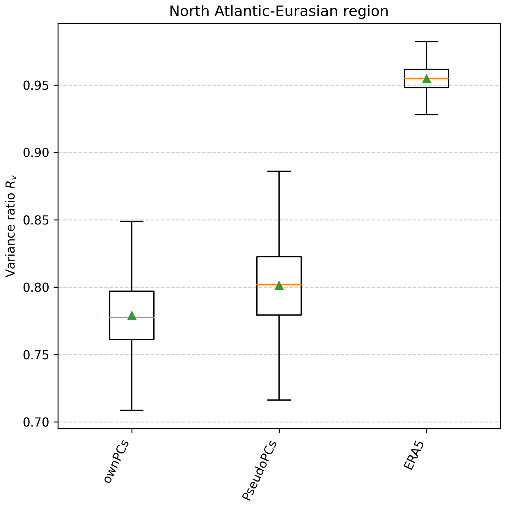
Figure A1 Variance ratio for Common circulation regime data projected onto reference state space (Pseudo PCs) and its own state space (own PCs) as well as ERA5. The box plots refer to the distribution of 15 years bootstraps (n=1000) of each model and show mean (triangle), median (horizontal line), first and third quartile (boxes) and 10 and 90 percentiles (bars).

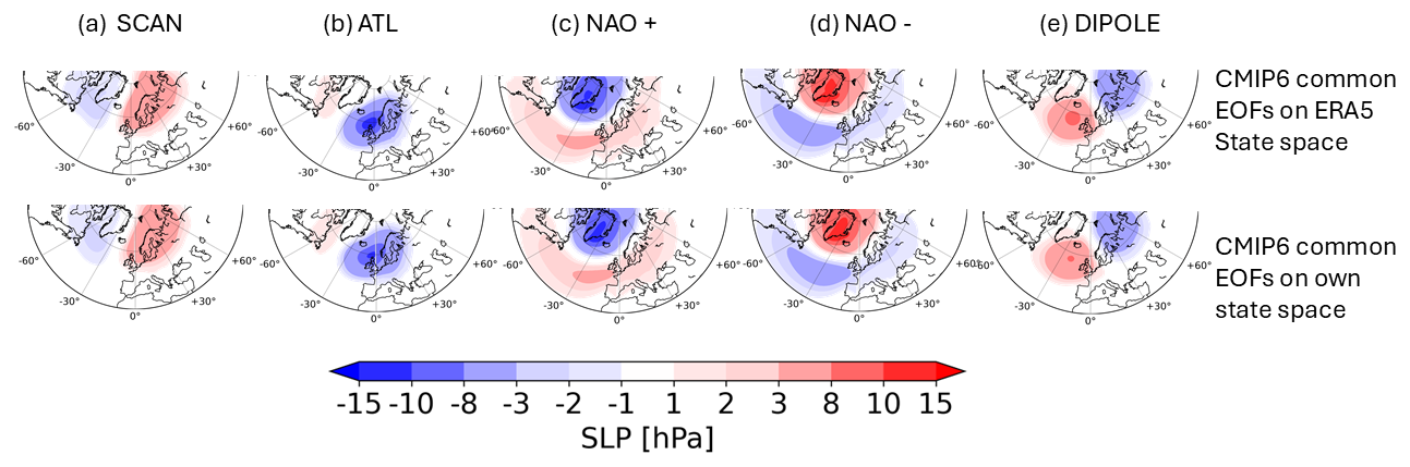
Figure A2 North-Atlantic Eurasian Circulation regime patterns in terms of SLP anomalies for MJJASO, for CMIP6 models in the historical period 1985-2014 obtained with K-Means clustering. Upper row: Common simulated circulation regime approach, with model data projected onto the ERA5 state space, lower row: Common regime approach with state space spanned by common EOFs from climate model data.

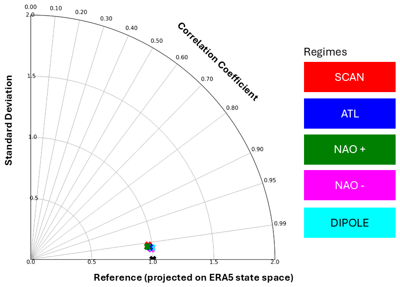
Figure A3 Common regime approach with state space spanned by common EOFs from climate model data compared to the reference of model data projected onto the ERA5 state space for the North-Atlantic Eurasian region.

Appendix B: List of Considered CMIP6 Climate Models

Table B1 lists the CMIP6 models that were examined in this study, along with their constituent ensemble members and relevant references.

Bi et al. (2020)Ziehn et al. (2020)Danabasoglu et al. (2020)Voldoire et al. (2019)Voldoire et al. (2019)Seferian (2018)Held et al. (2019)Dunne et al. (2020)Williams et al. (2018)Volodin et al. (2019)Boucher et al. (2020)Byun et al. (2019)Tatebe et al. (2019)Hajima et al. (2020)Mauritsen et al. (2019)Mauritsen et al. (2019)Yukimoto et al. (2019)Seland et al. (2020)Sellar et al. (2019)

Table B1 Examined CMIP6 models, their ensemble member, and the references.

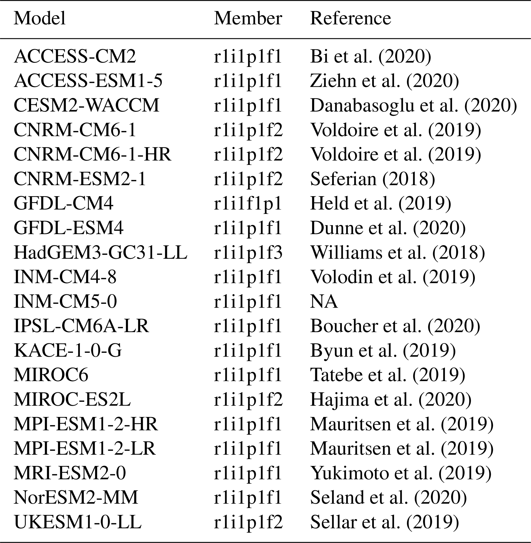
NA: not available.

Appendix C: Number of Considered Circulation Regimes

We have based the decision for a reasonable number of circulation regimes on three metrics: the anomaly correlation coefficient between the patterns of the clusters, the elbow test and the silhouette score.

C1 Anomaly Correlation Coefficient

The anomaly correlation coefficient (ACC) quantifies how well the spatial structure of one anomaly pattern corresponds to that of another pattern, independent of their absolute magnitudes. Following the criterion of Grams et al. (2017), the ACC can be used to assess the distinctiveness of weather regimes: if the correlation between different clusters remains below 0.4, the clusters can be considered sufficiently different to represent distinct regimes. In our analysis, we computed the ACC between clusters for the North Atlantic–Eurasian region and Arctic region in Fig. C1, applying both the KME and SAN methods to ERA5 data from 1985–2014. For both methods and both regions, the suggested threshold of Grams et al. (2017) is satisfied with five regimes, which supports our choice of this number of regimes.

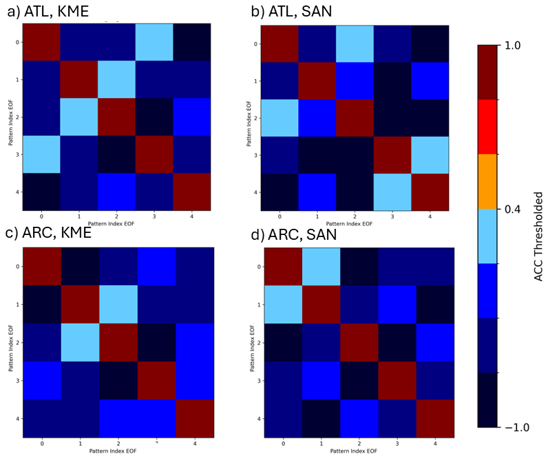
Figure C1 Anomaly correlation coefficient matrices for the North Atlantic–Eurasian regime patterns for KME method in (a), SAN in (b). The matrices considering the Arctic regimes are aligned below for KME in (c) or SAN in (d), all four using the reference ERA5 data in the historical time period 1985–2014.

C2 Elbow Plot

The following scores are specific to the KME algorithm. The Elbow plot (Olmo et al., 2024) illustrates the distortion score, which describes the within-cluster sum of squared distances and is often employed to assess the efficiency of the formation and allocation of centroids. The Distortion score is calculated using the KElbow Visualizer function from the Yellowbrick python project (https://www.scikit-yb.org, last access: 30 November 2025) (Fig. C2). The algorithm calculates the elbow point, which is defined as the point of greatest curvature in the curve. The KElbow Visualizer suggests that five clusters represent an optimal number of clusters for both regions, the North Atlantic–Eurasian and Arctic, for the extended boreal summer season from May to October.

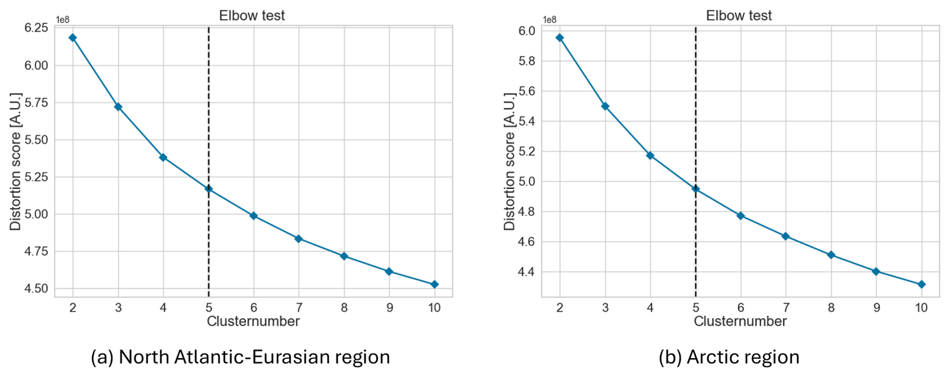
Figure C2 Distortion score of the dataset considered for the respective region. The row specifies the investigated region, the column shows the results for different numbers of clusters.

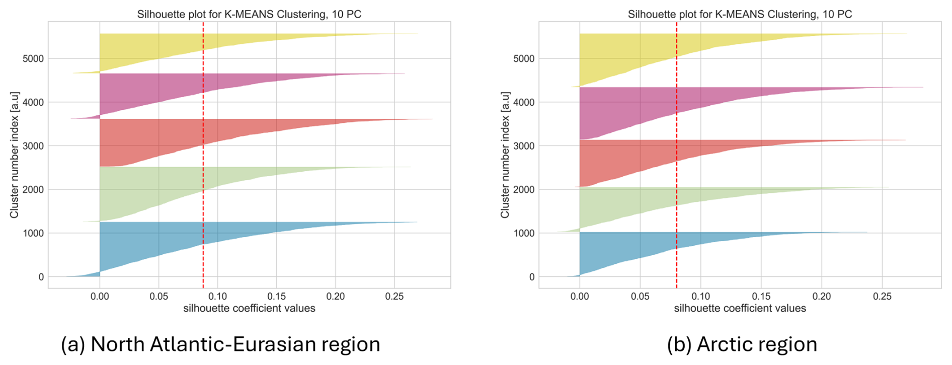
Figure C3 Silhouette plot North-Atlantic–Eurasian regimes (a) and Arctic regimes (b) determined with the KME method. The cluster number index represents the number of days assigned to the cluster centroids over the period 1985–2014, which total 5520 d.

C3 Silhouette Score

The silhouette score (Rousseeuw, 1987) is evaluated and illustrated in Fig. C3 for both regions. The silhouette score is a metric utilised to assess the quality of clustering, whereby the cohesion and separation of clusters are measured (https://scikit-learn.org/stable/modules/generated/sklearn.metrics.silhouette_score.html, last access: 30 November 2025). The average distance between data points within the same cluster is defined as cohesion, whereas the average distance between data points in one cluster and the nearest neighboring cluster is defined as separation. The silhouette coefficient value ranges from −1 to 1. A positive silhouette score indicates the presence of well-defined and separated clusters. Conversely, a negative score suggests the existence of overlapping or poorly defined clusters. The mean silhouette score for both regions is approximately 0.08, although the coefficient for the North Atlantic–Eurasian clusters is greater than that for the Arctic clusters. For each cluster number index, the silhouette coefficient value is positive, supporting the choice of 5 clusters for both regions.

Appendix D: Sensitivity Tests on Arctic Region

In contrast to the North Atlantic–Eurasian region, where Dorrington and Strommen (2020); Boé et al. (2009); Crasemann et al. (2017); Riebold et al. (2023) have considered similar regions, there is currently no consensus on the dimensions and confinement of the Arctic region to investigate within the circumpolar Arctic during the summer season (Proshutinsky et al., 2015; Wang et al., 2021; Timmermans and Marshall, 2020). If the region is defined too narrowly, for example, as 60 to 90° N, the resulting clusters are geometrically constrained, refer Fig. D1, bottom row. The storm track route is located approximately at 60°, leading to patterns that are more geometrical than physically reasonable if the investigated area is confined to 60° N. The aforementioned constraints are not observed when the region is extended to 50 or 40° N, where the calculated patterns from the K-Means algorithm exhibit a similar spatial structure refer to Fig. D1, center and top row. Therefore, the region under consideration is defined as the smallest area that still exhibits physical patterns in the Arctic region, spanning 50 to 90° N and covering the entire circumpolar region.

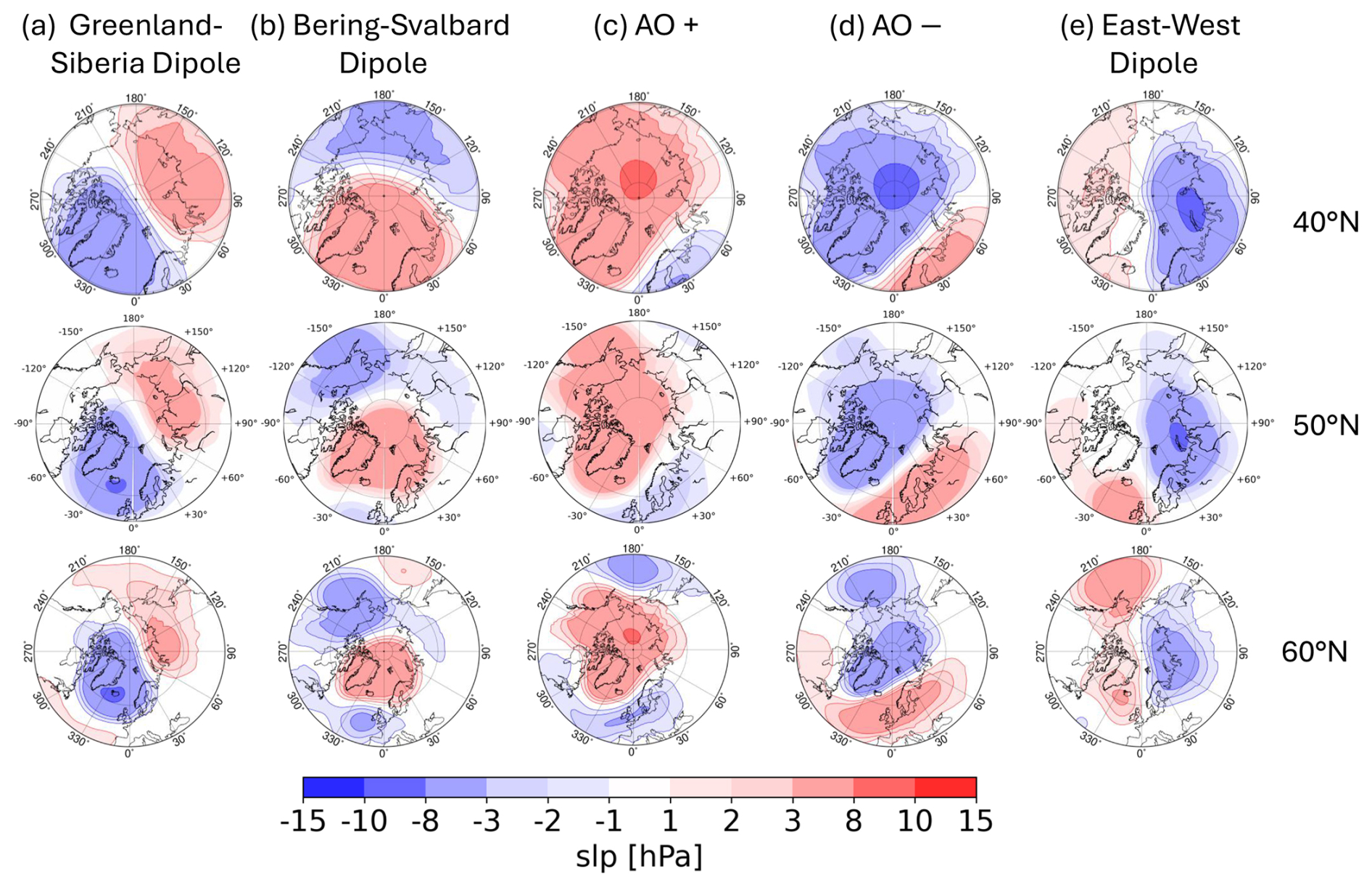
Figure D1 Reference circulation regimes ERA5 for the Arctic region in the historical time period 1985–2014 for different constraints calculated by the KME algorithm in the extended boreal summer season from May to October.

Appendix E: Additional climate variables composites

Just like with the zonal wind anomalies, the composites of temperature at 2 m and total precipitation anomaly (after preprocessing) composites are shown in Figs. E1–E4. It is evident that temperature, total precipitation, and wind patterns show strong similarities between the KME and SAN regimes in the North Atlantic–Eurasian region, as well as among the four regimes in the Arctic region. Moreover, an analysis of the respective anomalies, combined with the results on frequency of occurrence, reveals that the NAO+, DIPOLE, and AO− patterns are consistently associated with positive temperature anomalies over western North America. The feature has been also identified in CMIP3 data by Ray et al. (2008); McWethy et al. (2010). Furthermore, NAO+ and AO− are linked to dry (negative precipitation anomalies) and warm (positive temperature anomalies) conditions above Scandinavia and central Europe, and are projected to be more persistent under global warming. This predicted long-lasting dry and warm spells are also reported in Pfleiderer et al. (2019).

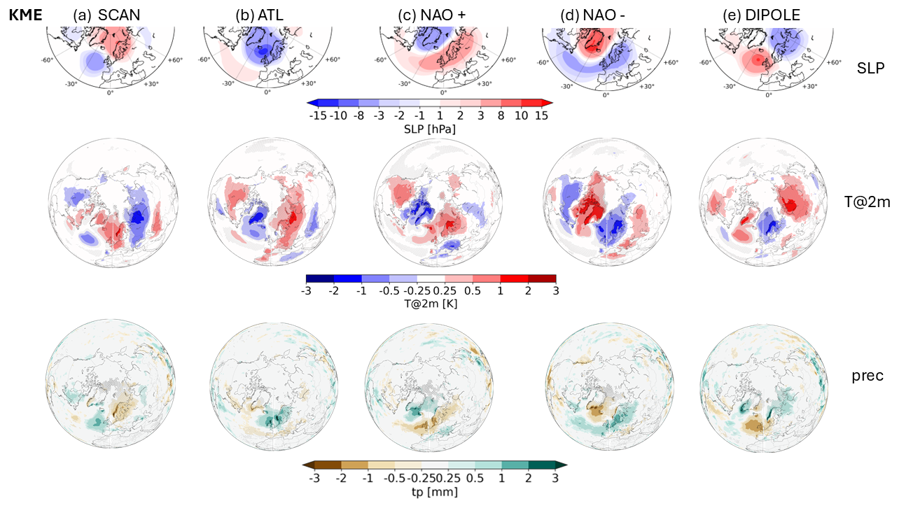
Figure E1 Reference circulation regimes in the historical time period computed from ERA5 dataset with the KME method in the upper row for the North Atlantic–Eurasian region. The center row indicated temperature composites at a height of 2 m in K. The lower row shows the total precipitation composites in mm.

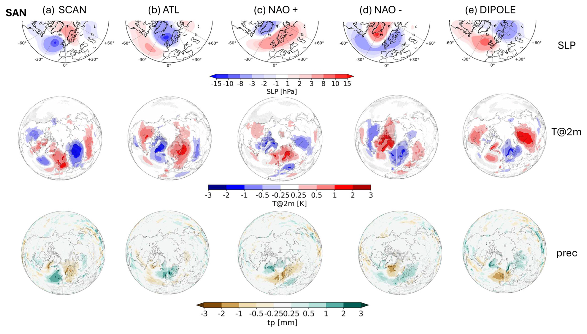
Figure E2 Similar to Fig. E1 but for the SAN method.

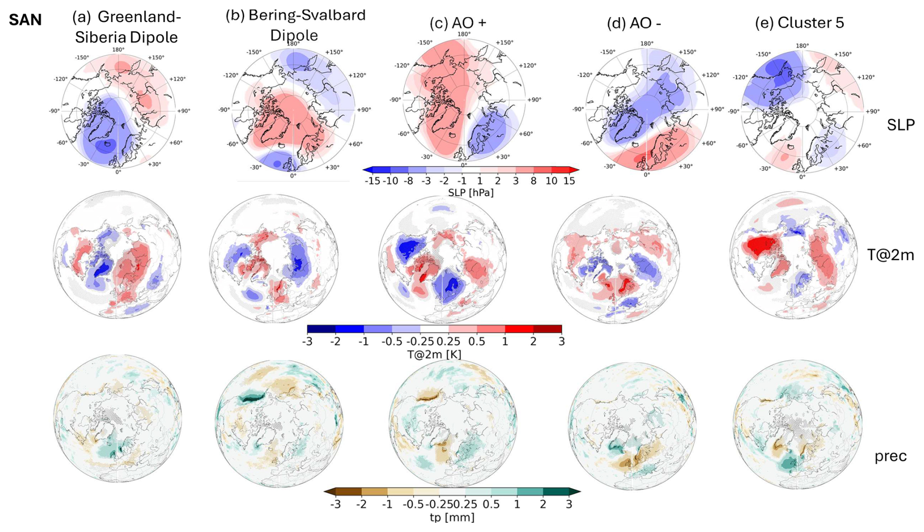
Figure E3 Reference circulation regimes in the historical time period computed from ERA5 dataset with the KME method in the upper row for the Arctic region. The center row indicated temperature composites at a height of 2 m in K. The lower row shows the total precipitation composites in mm.

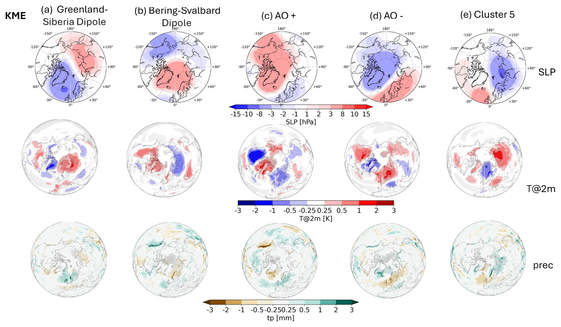
Figure E4 Similar to Fig. E3 but for the SAN method.

Appendix F: Zonal wind anomaly for SAN regimes

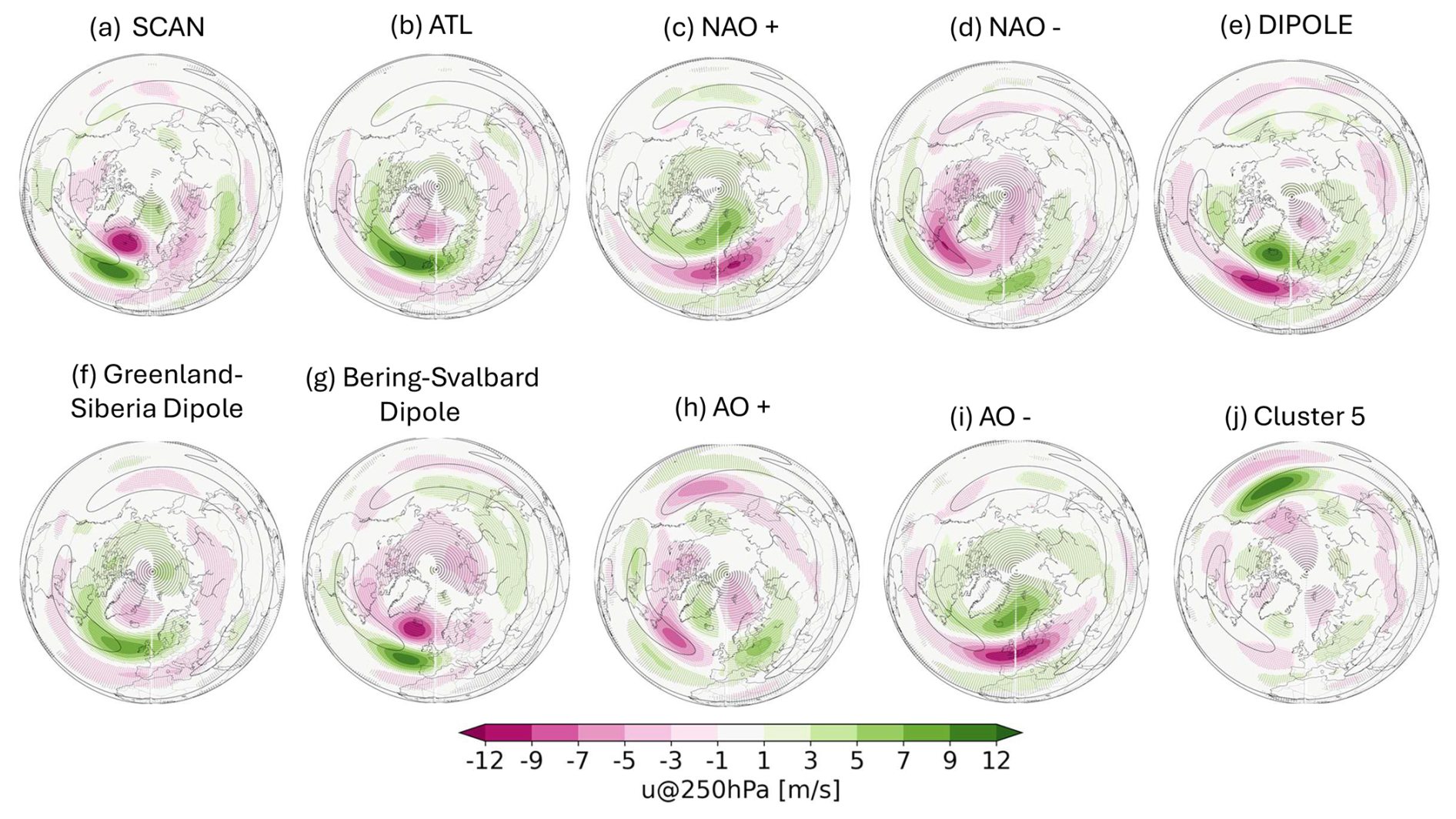
Figure F1 Zonal wind composites @250hPa for the SAN regimes for the North Atlantic–Eurasian region in the upper row and the Arctic region in the lower row.

The zonal wind anomaly composites at an height of 250 hPa computed for the SAN regimes are shown in Fig. F1. For the North Atlantic–Eurasian region, the wind composites look very similar to the KME regimes, refer to Fig. 2, lower row. Regarding the Arctic region, the spatial correlation for four regimes (except Cluster 5) indicates high similarity between KME and SAN regimes, that aligns with the findings for the wind composites. The spatial structure between Fig. 8 and the lower row in Fig. F1 is very similar but the amplitudes for wind anomalies are more different from each other, e.g. for AO−. For Cluster 5 the SLP patterns and linked wind composites exhibit low correlation and visual similarity, as the SAN Cluster 5 is characterized by a stronger Pacific jet exit and KME Cluster 5 is more dominated by a poleward shift in the Atlantic jet structure.

Appendix G: Multi-model Mean Change

Figure G1 shows the ensemble mean change in SLP.

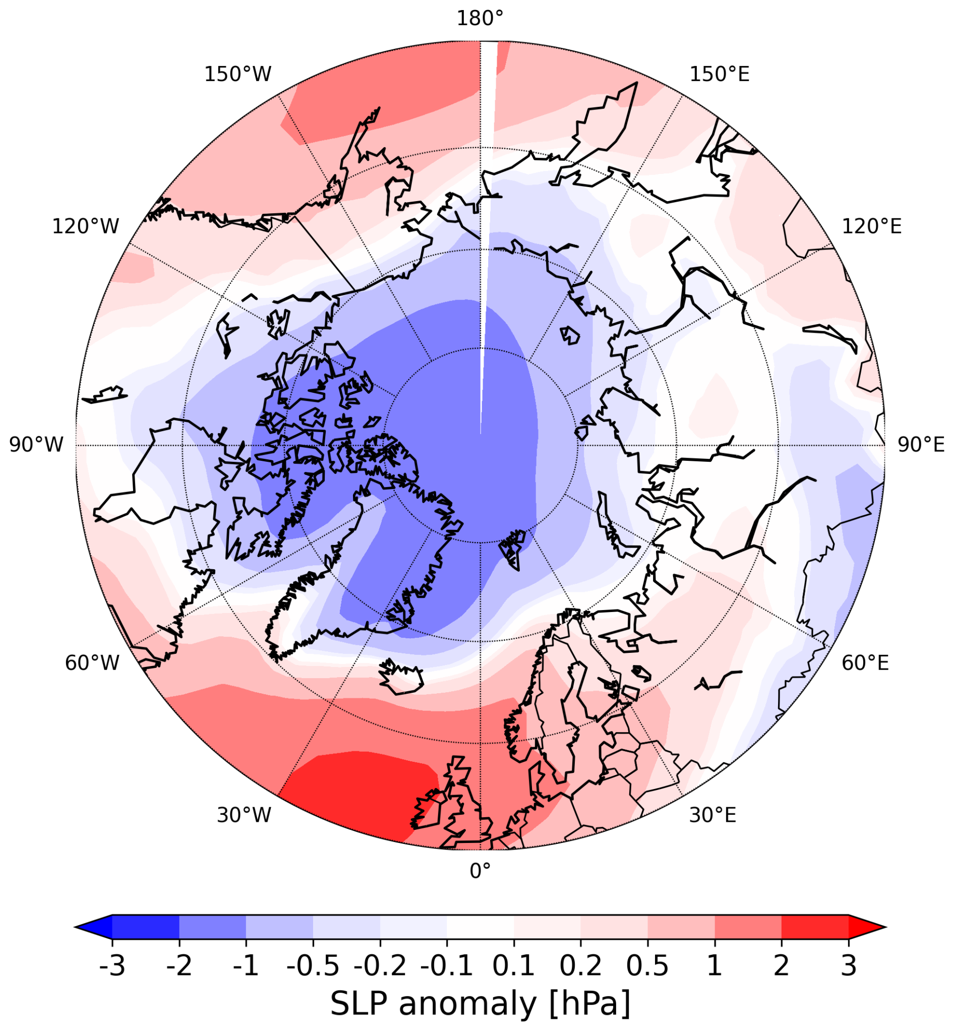
Figure G1 Multi-model mean change in SLP from historical to future period (2070–2099 minus 1985–2014) for the extended Boreal summer season (MJJASO).