CYCLOPs: a Unified Framework for Surface Flux-Driven Cyclones Outside the Tropics

Cyclonic storms resembling tropical cyclones are sometimes observed well outside the tropics. These include medicanes, polar lows, subtropical cyclones, Kona storms, and possibly some cases of Australian East Coast Lows. Their structural similarity to tropical cyclones lies in their tight, nearly axisymmetric inner cores, eyes, and spiral bands. Previous studies of these phenomena suggest that they are partly and sometimes wholly driven by surface enthalpy fluxes, as with tropical cyclones. Here we show, through a series of case studies, that many of these non-tropical cyclones have morphologies and structures that resemble each other and also closely match those of tropical transitioning cyclones, with the important distinction that the potential intensity that supports them is not present in the pre-storm environment but rather is locally generated in the course of their development. We therefore propose to call these storms CYClones from Locally Originating Potential intensity (CYCLOPs). We emphasize that mature CYCLOPs are essentially the same as tropical cyclones but their development requires substantial modification of their thermodynamic environment on short time scales. Like their tropical cousins, the rapid development and strong winds of CYCLOPs pose a significant threat and forecast challenge for islands and coastal regions, and the effects of climate change on them should be considered.

1 Introduction

Cyclones that resemble tropical cyclones are occasionally observed to develop well outside the tropics. These include polar lows, medicanes, subtropical cyclones, Kona storms (central North Pacific), and perhaps some cases of Australian East Coast Lows. The identification of such systems is usually based on their appearance in satellite imagery and on the environmental conditions in which they occur. Here we show that many of these systems are manifestations of the same physical phenomenon and, as such, should be given a common, physically-based designation. We propose to call these CYClones from Locally Originating Potential intensity (CYCLOPs), with reference to the one-eyed creatures of Greek mythology¹. We show that in many respects these developments resemble classical “tropical transition” (TT) events (e.g. Bosart and Bartlo, 1991), but they are distinguished from the latter by occurring in regions where the climatological potential intensity is small or zero. (Some events previously identified as TT events were probably examples of CYCLOPs.) Their often-rapid development and intense mesoscale inner cores, compared to extratropical cyclones, make CYCLOPs significant hazards and a forecasting challenge.

Cyclones of synoptic and sub-synoptic scale are powered by one or both of two energy sources: the available potential energy (APE) associated with isobaric temperature gradients (baroclinity), and fluxes of enthalpy (sensible and latent heat) from the surface (usually the ocean) to the atmosphere². A normal extratropical cyclone over land is an example of the former, while the latter is epitomized by a classical tropical cyclone. Extratropical transitioning and tropical transitioning cyclones³ can be powered by both sources, either in sequence or with the relative proportion varying over the life of the storm (see, e.g., Fantini, 1990). Additionally, we note that tropical cyclones often originate in disturbances, such as African easterly waves, that derive their energy from baroclinic and barotropic sources.

Like tropical cyclones, CYCLOPs are mainly powered by surface enthalpy fluxes, but differ from the former in that the required potential intensity is produced locally and transiently, whereas tropical cyclones develop in seasons and regions where sufficient potential intensity is always present. CYCLOPs closely resemble the strongly baroclinic cases of tropical transition defined and discussed by Davis and Bosart (2004), except that they occur in regions where the climatological potential intensity is too small for tropical cyclogenesis, relying on synoptic-scale perturbations that locally enhance potential intensity in space and time. Davis and Bosart (2004) confined their attention to tropical cyclone formation in regions of high sea surface temperature, stating that “The precursor cyclone must occlude and remain over warm water (26 °C) for at least a day following occlusion.” Similarly, McTaggart-Cowan et al. (2008) and McTaggart-Cowan et al. (2013) only examined cases of tropical transition that resulted in named tropical cyclones. But McTaggart-Cowan et al. (2015) recognized that around 5 % of the cases they identified as tropical transition cases occurred over colder water and that upper-level troughs played a key role in destabilizing the atmosphere with respect to the sea surface. We here build on this work and place it within the framework of potential intensity theory.

The basic physics of CYCLOPs was explored by the first author in reference to medicanes (Emanuel, 2005), and is illustrated in Fig. 1. While the actual evolution is, of course, continuous, it is simpler to discuss it in phases. For this narrow purpose, we assume that a cut-off cyclone has already formed in the upper troposphere, signified by the presence of an isolated potential vorticity (PV) anomaly near the tropopause (Fig. 1a). We show an idealized circularly symmetric anomaly and a cross-section through it; in practice, such developments are seldom close to axisymmetric in their earlier stages. In the illustration, the first phase is assumed to occur over land, but that need not be the case in general.

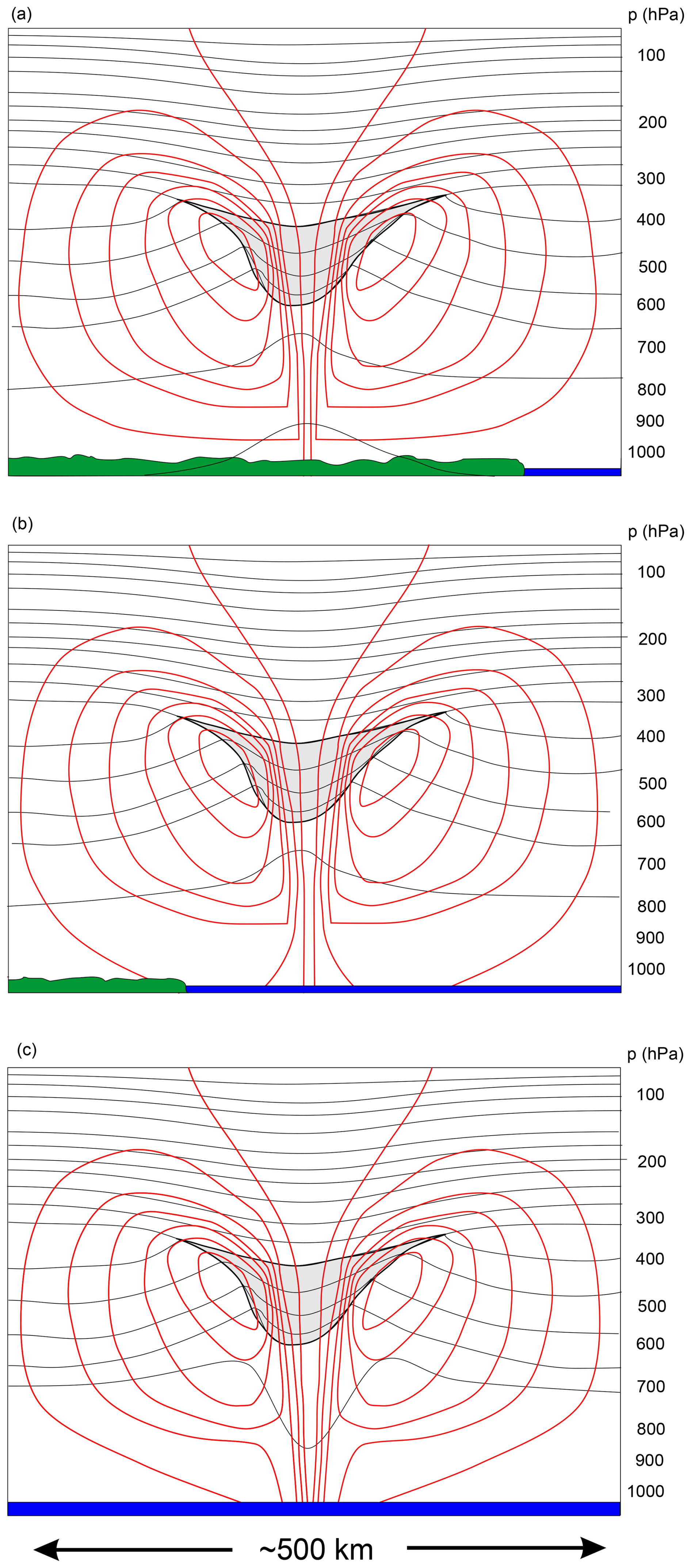
Figure 1 Three stages in the development of a CYCLOP. Each of the three panels shows a cross-section through an isolated PV anomaly at the tropopause (gray shading), idealized as circular. The thin black curves are isentropes, while the red curves are isotachs of the flow normal to the cross-section. In the first phase (a), the PV anomaly is over land, the troposphere beneath it is anomalously cold, and there may be no flow at the surface. The system moves out over open water in the next phase (b) and warming of the boundary layer and lower troposphere suffices to eliminate the cold anomaly at and near the surface. Weak cyclonic flow develops in response to the positive PV anomaly aloft. In the final phase (c), the surface heat fluxes become important and a tight, inner warm core develops.

During the creation of the near-tropopause PV anomaly, some combination of lifting and cold air seclusion has cooled and humidified the column underneath the PV anomaly, and the cold anomaly extends right to the surface. From a PV inversion perspective, the near-surface anticyclone that results from inverting the negative potential temperature anomaly at the surface is assumed to just cancel the cyclonic anomaly that results from inverting the tropopause PV anomaly, yielding no circulation at the surface. This assumption is made for simplicity here and we do not mean to imply that such a cancellation is common.

In phase 2 (Fig. 1b), the system drifts out over open water that is warm enough to diminish and eventually eliminate the cold anomaly at the surface, “unshielding” it from the PV anomaly aloft. During this phase, a cyclonic circulation develops in the lower troposphere, with a horizontal scale commensurate with that of the PV anomaly.

If the local potential intensity is large enough, and the air aloft sufficiently close to saturation, Wind-Induced Surface Heat Exchange (WISHE) can develop a tropical cyclone-like vortex (phase 3, Fig. 1c), with a warm inner core, eye and eyewall, and perhaps spiral bands. Note that the inner core may be warm only with respect to the synoptic-scale cold anomaly surrounding it, not necessarily with respect to the distant environment. At mid-levels, the temperature anomaly may manifest as a small-scale warm anomaly surrounded by a synoptic-scale cold anomaly.

In reality, these phases blend together into a continuum. Moreover, all three phases may (and often do) occur over water. One practical challenge is calculating the potential intensity. This should be calculated using the temperatures of the sea surface and the free troposphere under the PV anomaly aloft, but before the troposphere has appreciably warmed from surface fluxes. In practice, because the warming occurs either as the PV anomaly develops over water, or as it moves over water from land, we have no access to the sounding of the free troposphere before it has warmed up. The true potential intensity for a TC developing within the cold column under the PV anomaly is hence impossible to obtain. Nevertheless, we can estimate how cold the troposphere was before surface fluxes warmed it by using the surface pressure perturbation as a proxy for the CYCLOPs-induced warming, and assuming that the troposphere has an approximately moist adiabatic temperature profile⁴. This is derived in the Appendix. The result is a modified potential intensity, V_pm, given by

$$\begin{array}{}\text{(1)}& V_{\mathrm{pm}}^{\mathrm{2}}=V_{\mathrm{p}}^{\mathrm{2}}-{\displaystyle \frac{C_k}{C_{\mathrm{D}}}}{\displaystyle \frac{T_{\mathrm{s}}}{T_{\mathrm{400}}}}{\mathit{\varphi }}_{\mathrm{950}}{}^{\prime },\end{array}$$

where V_p is the potential intensity calculated in the usual way (e.g. Bister and Emanuel, 2002) from the local sea surface temperature and atmospheric sounding, ϕ₉₅₀^′ is the perturbation away from climatology of the near-surface geopotential, which we here evaluate at 950 hPa, C_k and C_D are the surface exchange coefficients for enthalpy and drag, and T_s and T₄₀₀ are the absolute temperatures at the surface and 400 hPa. As explained in the Appendix, we approximate the coefficient multiplying ϕ₉₅₀^′ in Eq. (1) by a constant value, 1.3, a reasonable estimate of the mean value of the coefficient. Note that Eq. (1) is only valid in places where our assumption that the lapse rate is moist adiabatic trough a deep layer is valid and deep moist convection occurs. Also, in the early stages of development, the outflow level is likely to be lower and the outflow temperature correspondingly higher, reducing the value of the coefficient multiplying ϕ₉₅₀^′ in Eq. (1).

Beginning with an upper cold cyclone in an environment of otherwise zero potential intensity, Emanuel (2005) simulated the development of a WISHE-driven cyclone using the axisymmetric, nonhydrostatic hurricane model of Rotunno and Emanuel (1987). The cold, moist troposphere under such an upper cyclone proves to be an ideal incubator of surface flux-driven cyclones with characteristics nearly identical to those of tropical cyclones. One interesting facet of the process is that the anomalous surface enthalpy flux destroys the parent upper cold low over a period of a few days, through the action of deep convection. This in another way in which CYCLOPs are distinguished from tropical cyclones, which tap spatially extensive regions of high potential intensity.

2 Why it matters

Why should we care whether a cyclone is driven by surface fluxes or baroclinity? From a practical forecasting standpoint, the spatial distributions of weather hazards, like rain and wind, can be very different, as can be the development time scales and fundamental predictability.

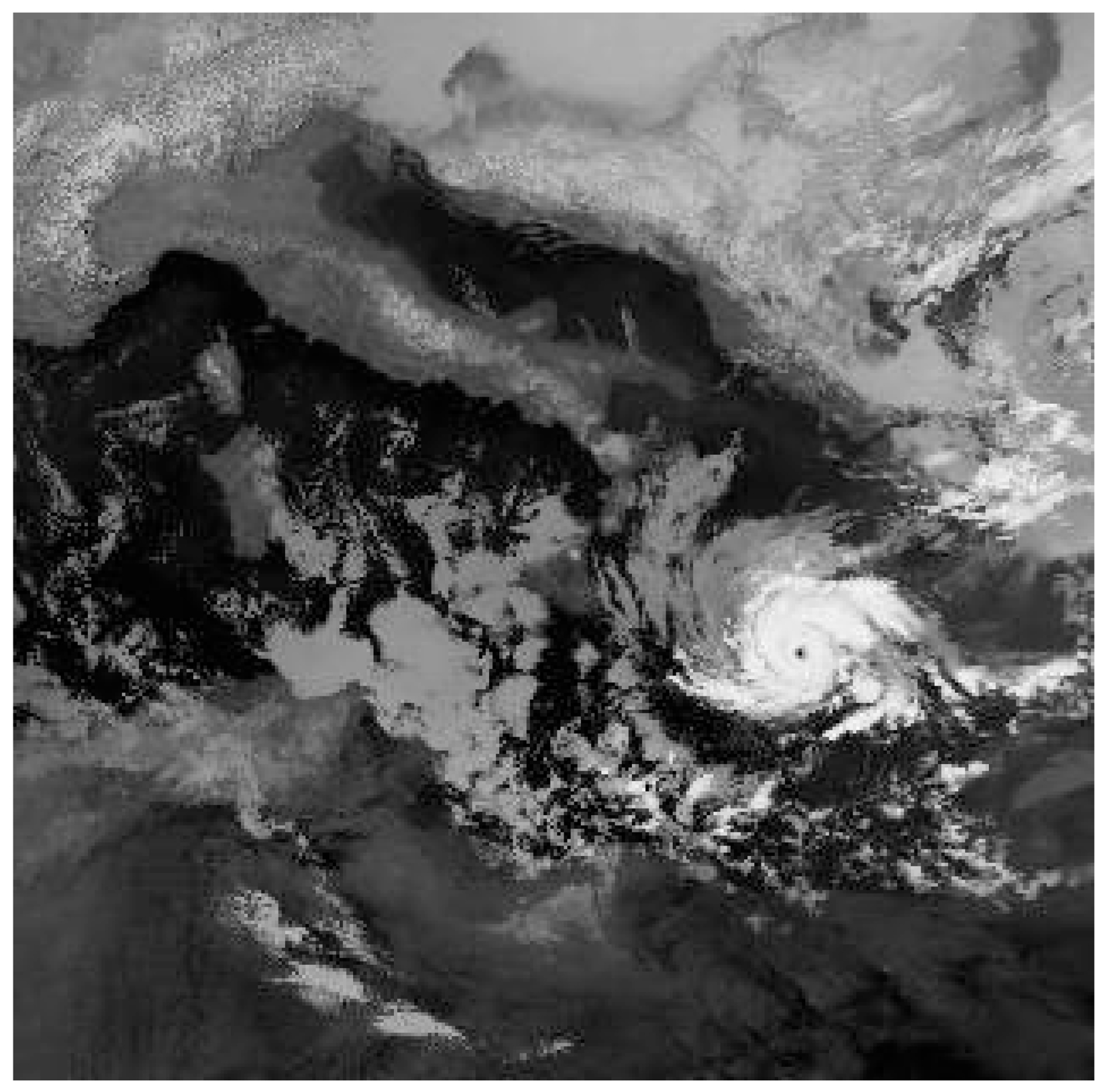
Figure 2 Infrared satellite image of Medicane Celeno in the central Mediterranean, at 09:06 UTC 16 January 1995. (Image credit: NOAA, 1995).

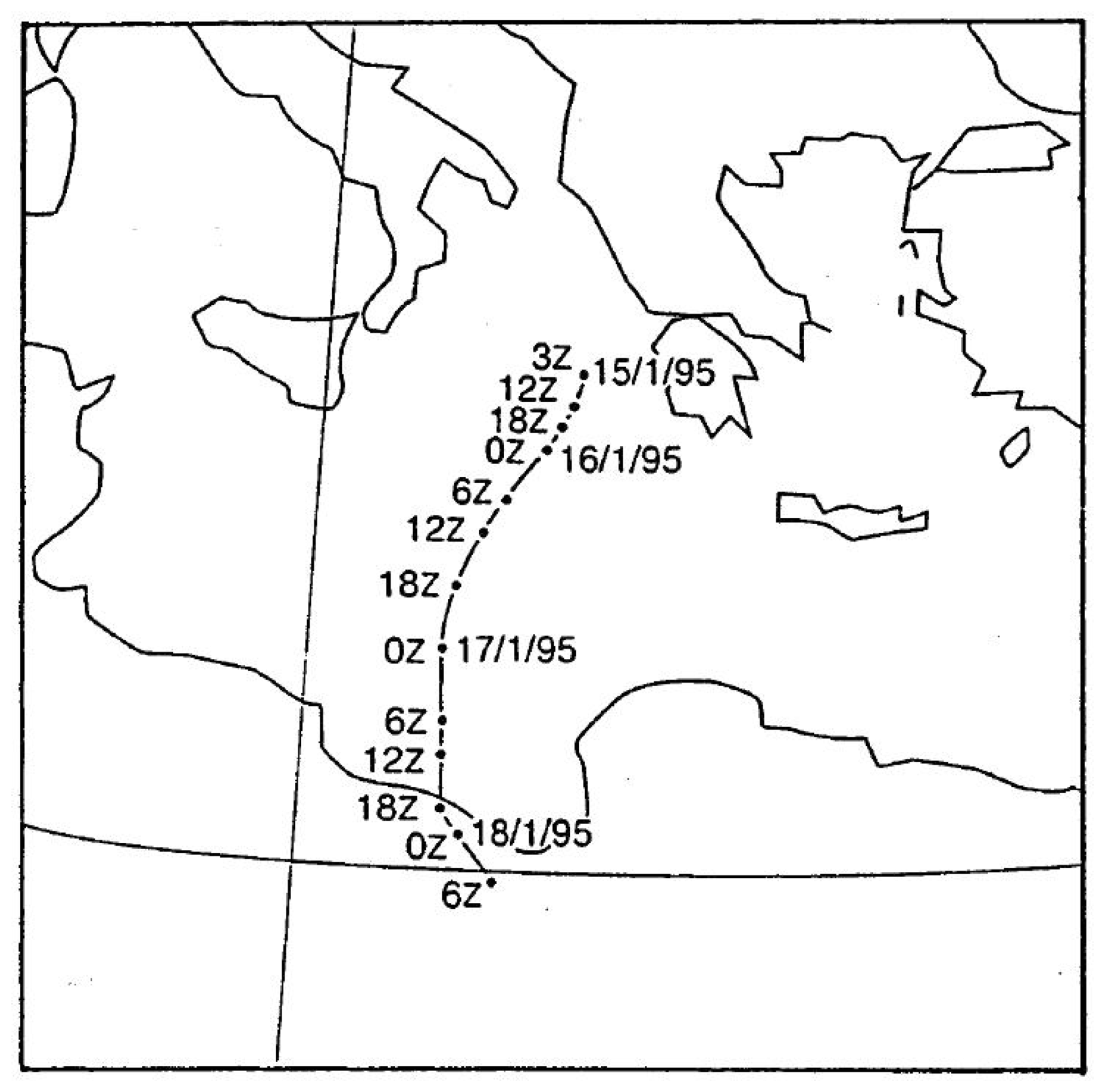
Figure 3 Track of the surface center of the cyclone between 03:00 UTC on 15 January and 06:00 on 18 January 1995, derived from satellite images (Pytharoulis et al., 1999).

In classical baroclinic cyclones, the strongest winds are often found in frontal zones and can be far from the cyclone center, while precipitation is usually heaviest in these frontal zones and in a shield of slantwise ascent extending poleward from the surface cyclone. There is long experience in forecasting baroclinic storms, and today's numerical weather prediction (NWP) of these events has become quite accurate, even many days ahead. Importantly, baroclinic cyclones are well resolved by today's NWP models. While baroclinic cyclones can intensify rapidly, both the magnitude and timing of intensification are usually forecast accurately, and uncertainties are well quantified by NWP ensembles (Leutbecher and Palmer, 2008).

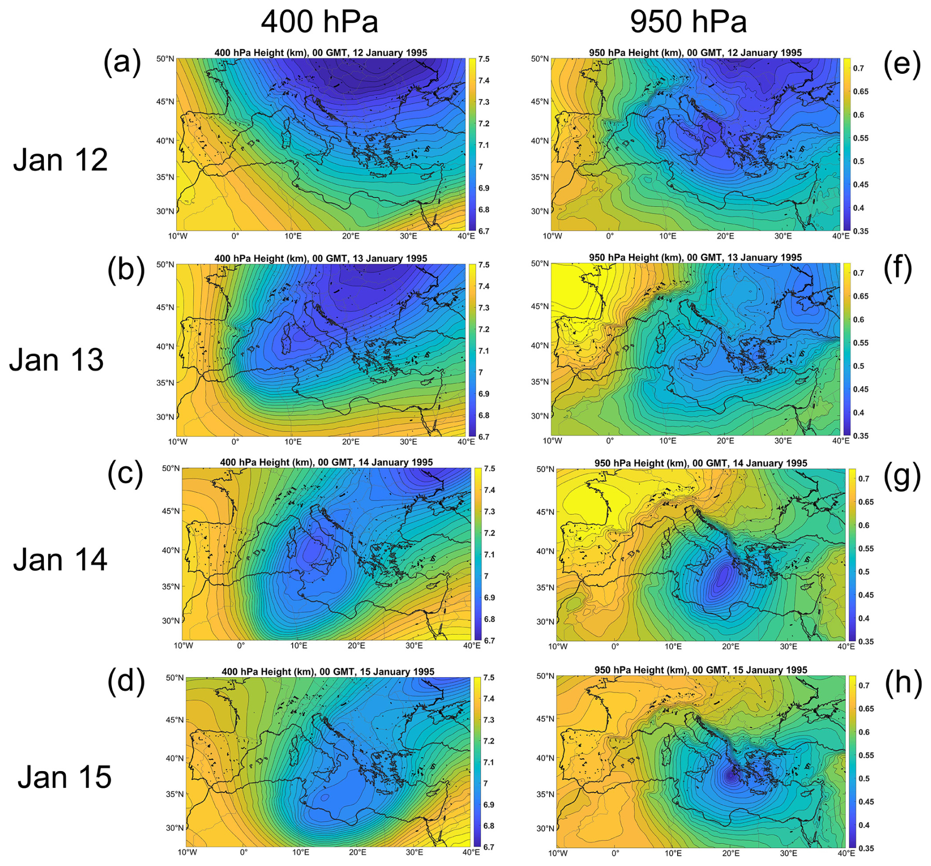
Figure 4 Evolution of the 400 hPa (left) and 950 hPa (right) geopotential heights in 24 h increments, from 00:00 UTC 12 January to 00:00 UTC 15 January 1995. These fields are from ERA5 reanalysis. The 400 hPa heights span from 6.7 to 7.5 km at increments of 26.67 m, while the 950 hPa heights range from 350 to 730 m at increments of 12.67 m.

By contrast, the physics of tropical cyclone intensification, involving a positive feedback between surface winds and surface enthalpy fluxes, results in an intense, concentrated core with high winds and heavy precipitation (which can be snow in the case of polar lows). The eyewalls of surface flux-driven cyclones are strongly frontogenetical (Emanuel, 1997), further concentrating wind and rain in an annulus of mesoscale dimensions. The intensity of surface flux-driven cyclones can change very rapidly and often unpredictably, presenting a severe challenge to forecasters. For example, Hurricane Otis of 2023 intensified from a tropical storm to a Category 5 hurricane in about 30 h, devastating Acapulco, Mexico, with little warning from forecasters. The small size of the core of high winds and heavy precipitation means that small errors in the forecast position of the center of the storm can lead to large errors in local wind and precipitation predictions. Surface flux-driven cyclones are too small to be well resolved by today's global NWP models, and even if they were well resolved, fundamental predictability studies show high levels of intrinsic unpredictability of rapid intensity changes (Zhang et al., 2014).

The time and space scales of surface flux-driven cyclones are such that they couple strongly with the ocean, producing near-inertial currents whose shear-driven turbulence mixes to the surface generally (but not always) colder water from below the surface mixed layer. This has an important (usually negative) feedback on the intensification of such cyclones. Accurate numerical forecasting of surface flux-driven cyclones therefore requires an interactive ocean, generally missing from today's NWP models because it is not very important for baroclinic cyclones and because of the additional computational burden.

For these reasons, it matters (or should matter) to forecasters whether a particular development is primarily driven by surface fluxes or by ambient baroclinity. The structural differences described above are often detectable in satellite imagery; at the same time, such imagery is sometimes misleading about the underlying physics. For example, classical baroclinic development sometimes develops cloud-free eyes surrounded by convection through the warm seclusion process, even over land, and yet may not have the intense annular concentration of wind and rain characteristic of surface flux-driven cyclones (Tous and Romero, 2013).

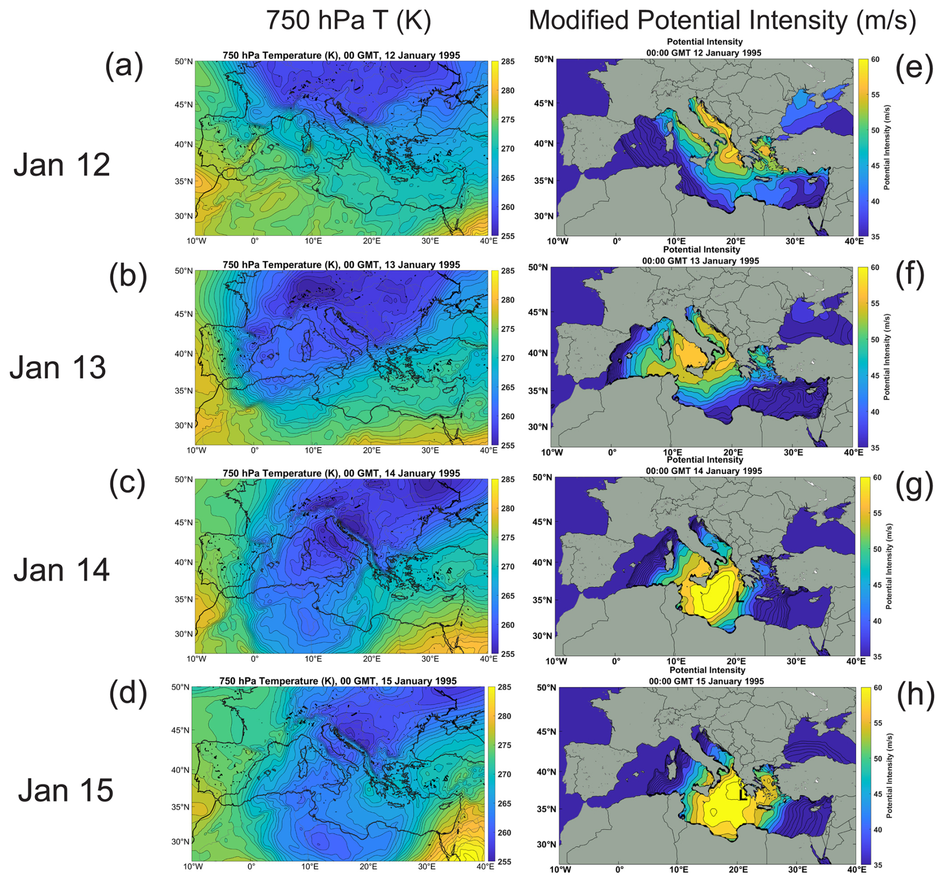
Figure 5 750 hPa temperature (K; left) and modified potential intensity given by Eq. (1) (m s⁻¹, right) at 00:00 UTC on 12–15 January (top to bottom) 1995. The 750 hPa temperature spans from 255 to 285 K at increments of 1 K, while the modified potential intensity ranges from 35 to 60 m s⁻¹ at increments of 4 m s⁻¹. The black “L”s in panels (g) and (h) show the positions of the surface cyclone. From ERA5 reanalysis.

3 Case Studies

Armed with the conceptual CYCLOP model developed in Section 1 and modified potential intensity given by Eq. (1), we now turn to case studies of the development of medicanes, polar lows, a subtropical cyclone, and a Kona storm, showing that the dynamic and thermodynamic pathways are similar. Specifically, each case developed after the formation of a deep, cold-core cut-off cyclone in the upper troposphere that often resulted from a Rossby wave breaking event. The lifting of the tropospheric air in response to the developing potential vorticity anomaly near the tropopause created a deep, cold, and presumably humid column. The deep cold air over bodies of relatively warmer water substantially elevates potential intensity, while its high relative humidity discourages evaporatively driven convective downdrafts, which tamp down the needed increase in boundary layer enthalpy. Low vertical wind shear near the core of the cutoff cyclone, coupled with high potential intensity and humidity, provide an ideal embryo for tropical cyclone-like development. The requirement for low vertical wind shear may prevent open troughs from producing CYCLOPs, even if the potential intensity is elevated.

In what follows, we focus on the cut-off cyclone evolution and the development of modified potential intensity. In a particular case, we compare reanalysis column water vapor to that estimated from satellite measurements. The differences between these are significant enough to cast some doubt on the quality of reanalyzed water vapor associated with the small-scale CYCLOP developments, thus we do not focus on water vapor even though it is known to be important for intensification of tropical cyclones.

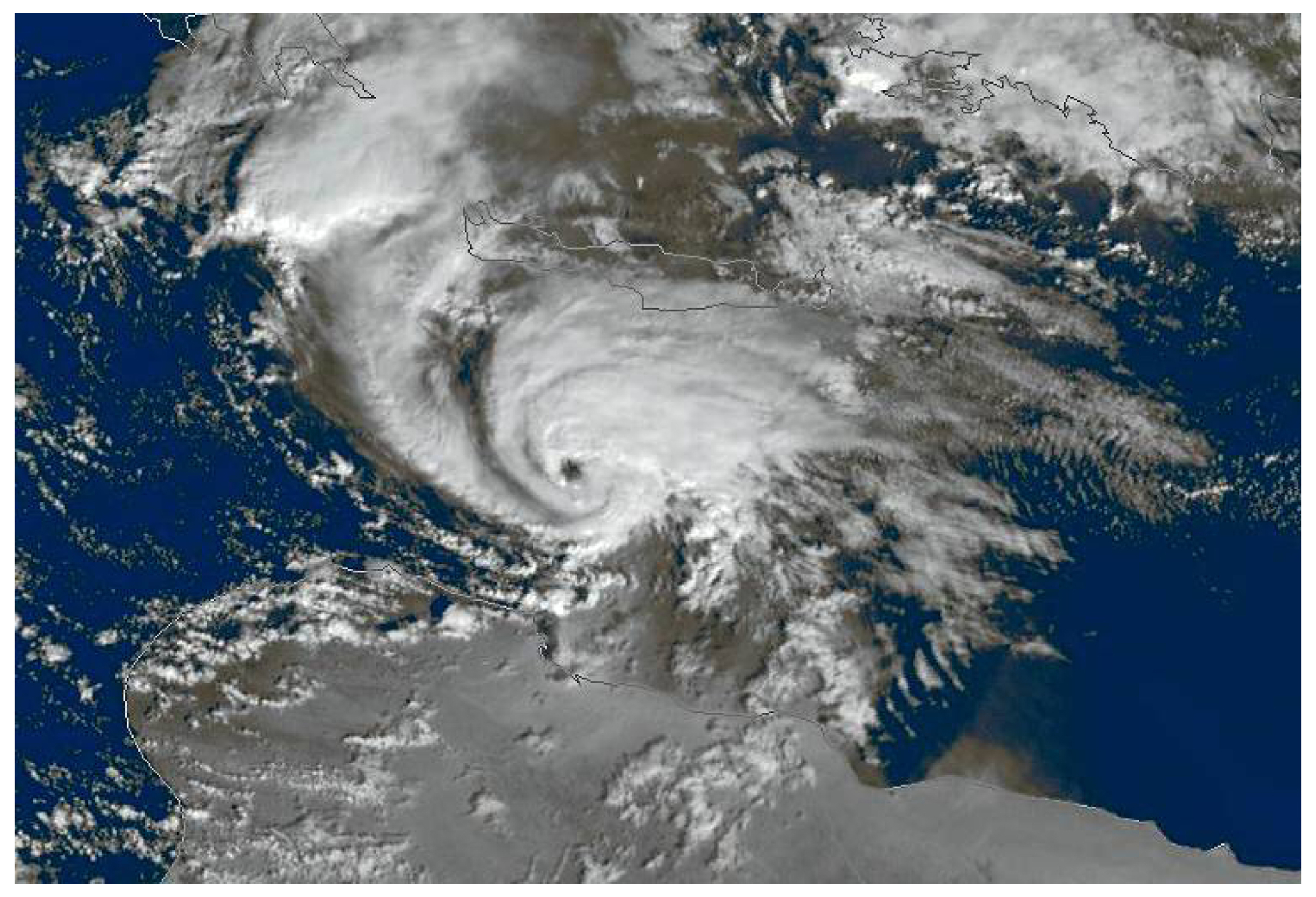
Figure 6 Medicane Zeo between Crete and Libya on 15 December 2005. Image from NASA.

We also examined, but do not show here, several cases of Australian East Coast Lows (Holland et al., 1987). Owing to the East Australian Current, the climatological potential intensity is substantial off the southeast coast of Australia, and the CYCLOP developments we analyzed behaved more like classical tropical transitions, with little or no role of the synoptic scale dynamics in enhancing the existing potential intensity. We suspect that there may be other cases in which the latter process was important, but did not conduct a search for such cases. It is clear that in many of these cases surface heat fluxes were important in driving the cyclone (Cavicchia et al., 2019). We also examined a small number of subtropical cyclones that developed in the South Atlantic, but as with the Australian cases, they resembled classical tropical transitions, though again we suspect there may be CYCLOP cases there as well.

As with tropical cyclones, there are variations on the theme of CYCLOPs, and we explore these in the closing sections.

3.1 Medicane Celeno of January 1995

On average, 1.5 medicanes are observed annually in the Mediterranean (Cavicchia et al., 2014; Nastos et al., 2018; Romero and Emanuel, 2013; Zhang et al., 2021) and, more rarely, similar storms are observed over the Black Sea (Yarovaya et al., 2008). We begin with a system, Medicane Celeno, that reached maturity on 16 January 1995, shown in infrared satellite imagery in Fig. 2.

Figure 3 shows the track of the surface center of the cyclone, which developed between Greece and Sicily and made landfall in Libya. A detailed description of this medicane is provided by Pytharoulis et al. (1999).

The evolution of the system in increments of 24 h, beginning on 00:00 UTC, 12 January and ending at 00:00 UTC 15 January, is shown in Fig. 4. This sequence, showing the 400 and 950 hPa geopotential heights, covers the period leading up to the CYCLOP development. The evolution of the upper tropospheric (400 hPa) height field shows a classic Rossby wave breaking event (McIntyre and Palmer, 1983) in which an eastward-moving baroclinic Rossby wave at higher latitudes amplifies and irreversibly breaks to the south and west, finally forming a cut-off cyclone. It is important to note that the formation of a cut-off cyclone in the upper troposphere involves a local conversion from kinetic to potential energy, with deep cooling associated with dynamically forced ascent (Gan and Piva, 2016). To the southeast of this trough, a weak, broad area of low geopotential height develops at 950 hPa mostly over land in a region of low-level warm advection. As the cold air under the cut-off low is gradually heated by the underlying sea, a broad surface cyclone develops by 00:00 UTC on 14 January. At around this time, the feedback between surface wind and surface enthalpy fluxes is strong enough to develop a tight inner warm core (warm, that is, relative to the surrounding cold pool, not necessarily to the unperturbed larger scale environment) and by 00:00 UTC on 15 January, it is noticeable just to the west of northwestern Greece (Fig. 5d). At the same time, the upper cold core weakens, perhaps aided by the strong heating from the surface transferred aloft by deep convection.

Figure 5 shows the corresponding evolution of the 750 hPa temperature and the modified potential intensity, V_pm, given by Eq. (1). The latter is only shown in the range of 35 to 60 m s⁻¹. Experience shows that tropical cyclone genesis is rare when the potential intensity is less than about 35 m s⁻¹ (Emanuel, 2010).

On 12 January, relatively small values of V_pm are evident in the eastern and northern Mediterranean, but with higher values developing over the northern Adriatic as cold air aloft creeps in from the north. As the upper tropospheric Rossby wave breaks and a cut-off cyclone develops over the central Mediterranean, V_pm increases greatly during 13 and 14 January, with peak values greater than 60 m s⁻¹. The CYCLOP develops in a region of high V_pm, though not where the highest values occur, until 15 January at which time the mature CYCLOP location corresponds to that of the highest V_pm. Note that a lower warm core is not obvious at 750 hPa until 15 January and that it occurs on a somewhat smaller scale than the cut-off cyclone.

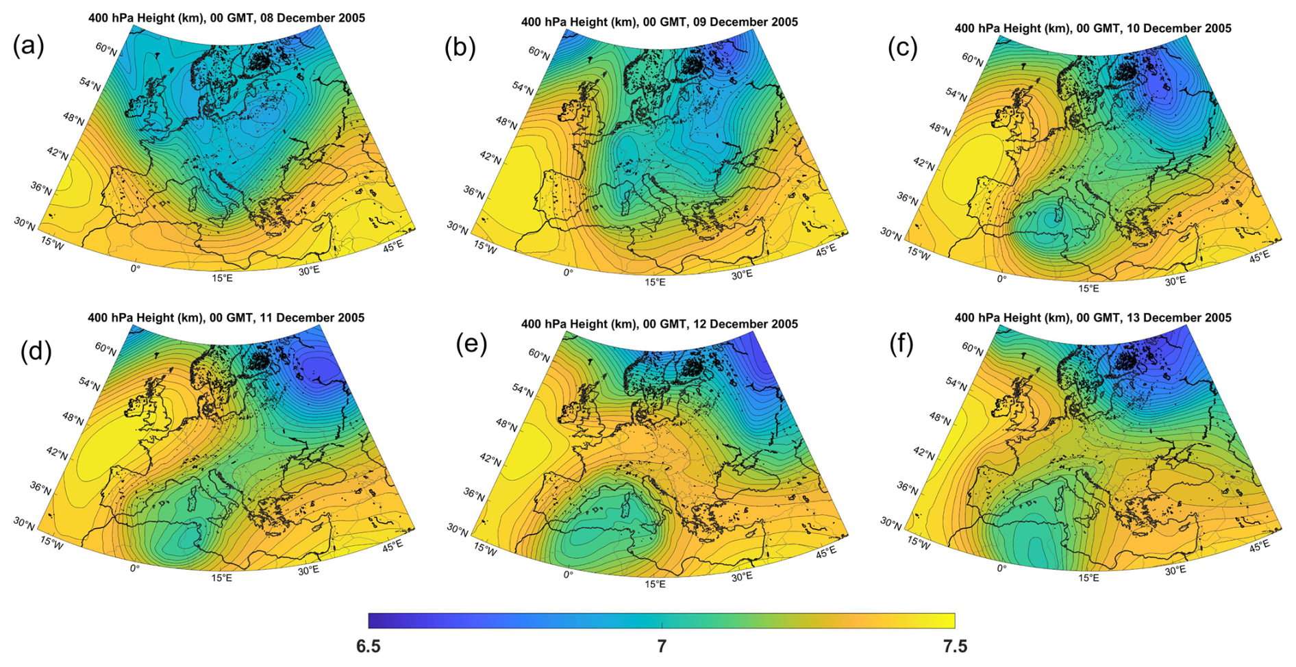
Figure 7 400 hPa geopotential heights, ranging from 6.5 to 7.5 km (color scale identical for all panels) at 00:00 UTC on 8 December (a), 9 December (b), 10 December(c), 11 December (d), 12 December (e), and 13 December (f), 2005. From ERA-5 reanalysis. Contour interval is 33.3 m.

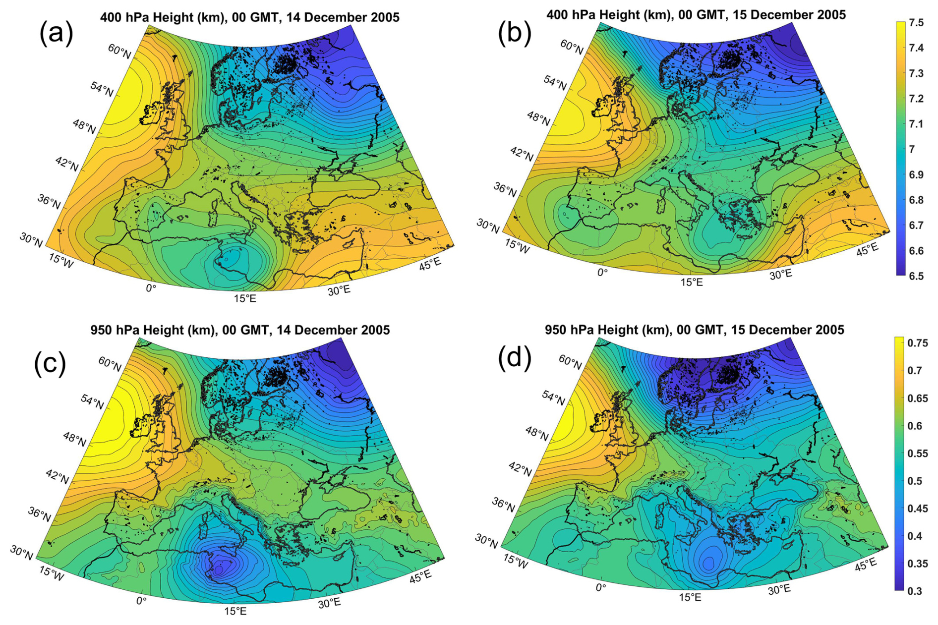
Figure 8 Evolution of 400 hPa geopotential height, ranging from 6.5 to 7.5 km at contour interval of 36.7 m (a, b), and 950 hPa geopotential height, ranging from 250 to 750 m at contour interval of 16.67 m (c, d) at 00:00 UTC in 14 December (a, c) and 15 (b, d), 2005. The color scales of (a) and (b) are identical, as are the color scales of (c) and (d). From ERA-5 reanalysis.

Figure A1 of the Appendix shows the individual contributions, on 14 and 15 January, of the usual potential intensity (first term on the right side of Eq. 1) and the correction for column warming (second term on right of Eq. 1) to the full potential intensity. (The contribution of column warming was negligible before 14 January) Note that the full potential intensity shown in Fig. 5 g and h is not the arithmetic sum of the two contributions but rather their Euclidean norm. The contribution of the column warming, as measured by the surface pressure anomaly, is quite localized around the CYCLOP and is located eastward of the maximum of the usual potential intensity.

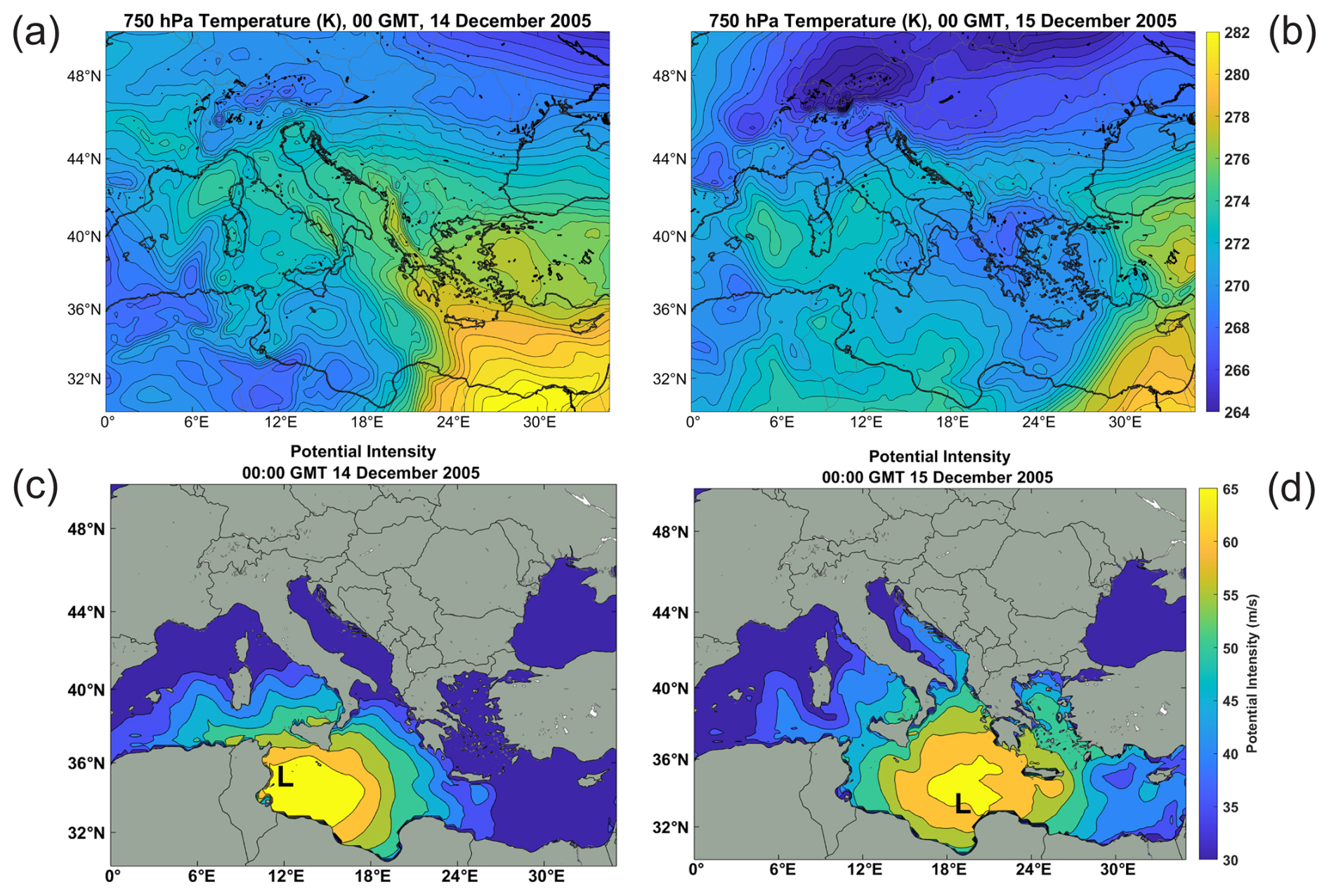
Figure 9 750 hPa temperature at increments of 0.6 K (a–b) and modified potential intensity from 35 to 65 m s⁻¹ at increments of 5 m s⁻¹ (c–d) at 00:00 UTC on 14 December (a, c) and 15 December (b, d) 2005. From ERA-5 reanalyses. The “L”s in (c) and (d) indicate the position of the 950 hPa cyclone center.

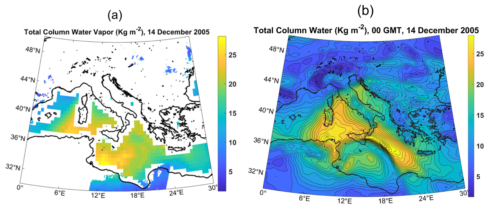
Figure 10 Total column water vapor (kg m⁻²) at 00:00 UTC on 14 December 2005, derived from microwave and near infrared imagers (a) and ERA5 reanalysis (b). In (b) the contour increment is 0.9 kg m⁻².

As the CYCLOP moves southward, it maintains a tight inner warm core until after landfall (not shown here) and the modified potential intensity, V_pm, over the south-central Mediterranean diminishes rapidly, with peak values of only about 50 m s⁻¹ by 00:00 UTC on 16 January. One potentially important difference between CYCLOP development and tropical transition is that in the former case, the volume of air with appreciable potential intensity is limited. It is possible that, by warming the whole tropospheric column relative to the surface, the enhanced surface fluxes associated with the CYCLOP, acting through deep convection, substantially diminish the magnitude and/or volume of the high V_pm air, serving to limit the lifetime of the CYCLOP. This was the case in the axisymmetric numerical simulations of Emanuel (2005).

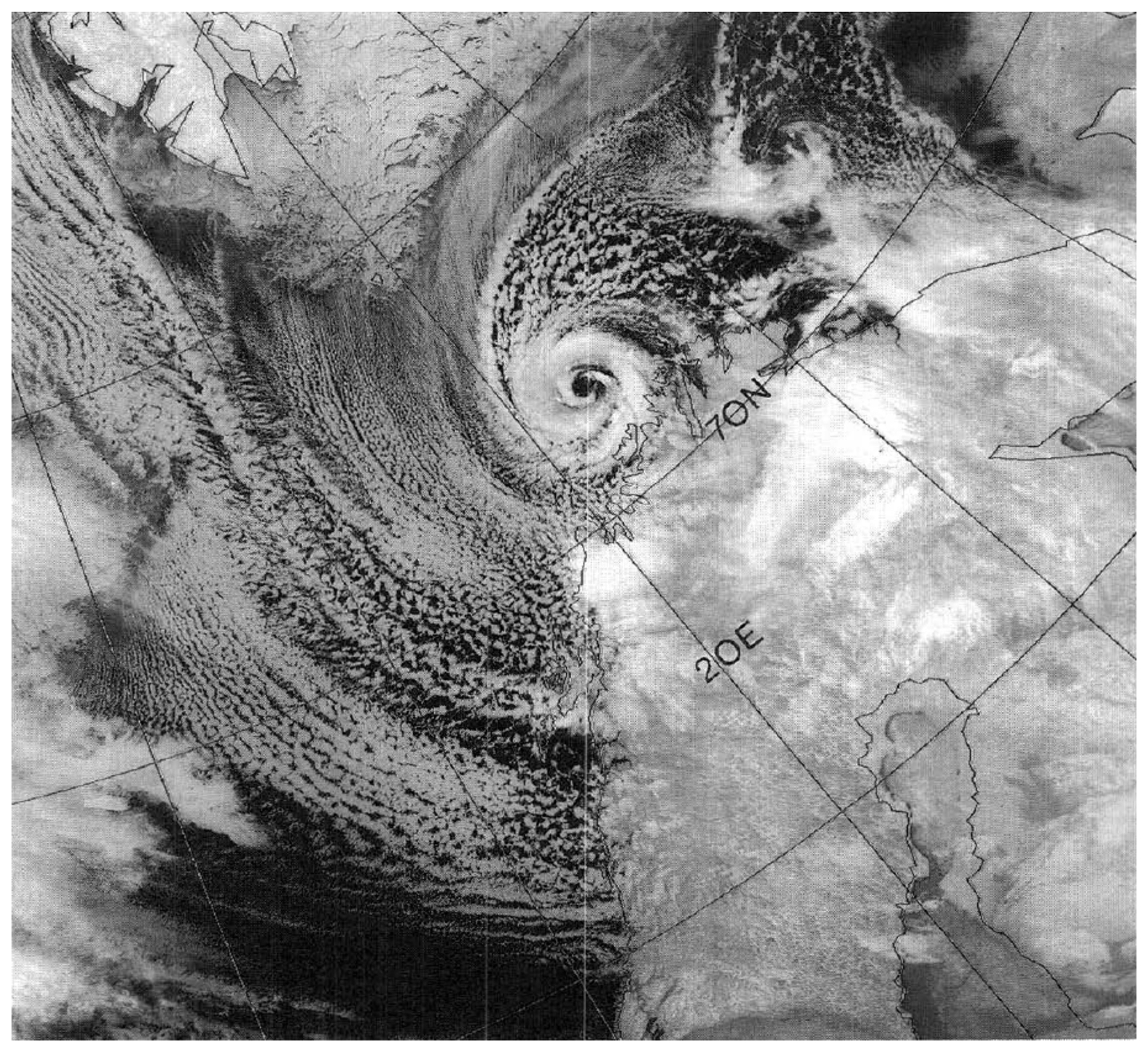
Figure 11 NOAA 9 satellite infrared image (channel 4) of a polar low just north of Norway at 08:31 UTC on 27 February 1987.

It is clear that this CYCLOP development occurred on time and space scales appreciably smaller than those of the rather weak, synoptic-scale cyclogenesis resulting from the interaction of the positive PV perturbation near the tropopause with a low-level temperature gradient. It is also clear that the strong cooling of the troposphere in response to the development and southward migration of the cutoff cyclone aloft was instrumental in bringing about the high potential intensity necessary to activate the WISHE process. Therefore, the Rossby wave breaking did much more than trigger cyclogenesis; it provided the necessary potential intensity for the CYCLOP development. Here we draw a distinction from tropical transition, in which, in most cases, the pre-existing potential intensity suffices to maintain a surface flux-driven cyclone. We emphasize again that there is a gray area here consisting of flux-driven cyclones in which the existing reservoir of potential intensity is enhanced to some degree by the local synoptic-scale dynamics.

3.2 Medicane of December 2005

A medicane, unofficially known as Zeo, formed on 14 December 2005 off the coast of Tunisia and then moved eastward across a large stretch of the Mediterranean. Figure 6 shows a satellite image of this medicane on 15 December. This cyclone has been the subject of several intensive studies (e.g. Fita and Flaounas, 2018; Miglietta and Rotunno, 2019).

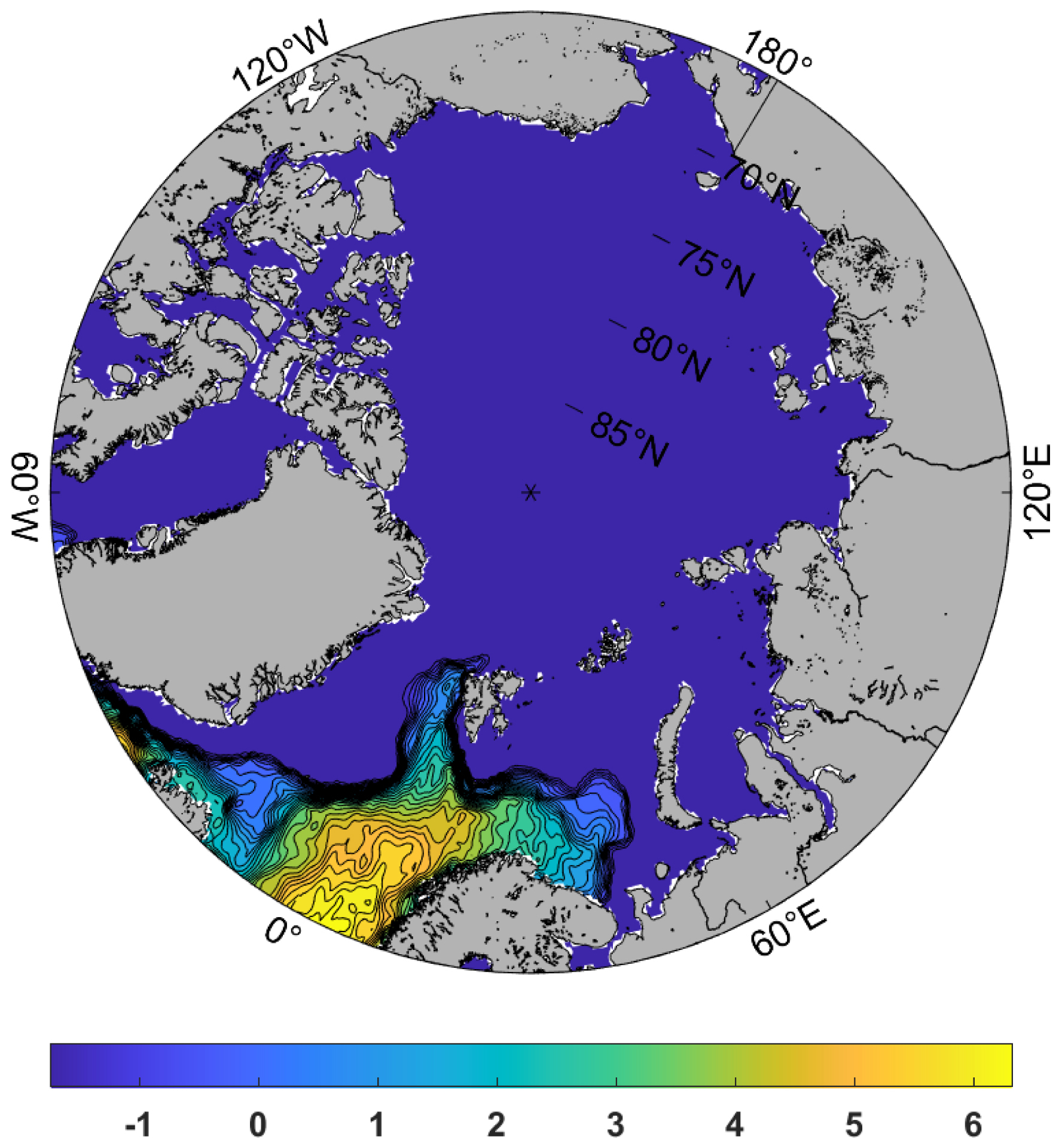
Figure 12 Sea surface temperature (°C) in intervals of 0.3 °C at 02:00 UTC on 25 February 1987, from ERA5 reanalysis. Dark blue areas denote regions of sea ice. From ERA-5 reanalyses.

Like Medicane Celeno, Medicane Zeo formed as a result of a Rossby wave breaking event, as illustrated in Fig. 7. On 8 December (panel a), a deep trough is digging southward over eastern Europe, but by 9 December (panel b) it has split in two, with the westward half breaking southwestward over Germany and Switzerland. By 11 December (panel d), this local minimum is located over Tunisia and on 12 December (panel e) it is more or less completely cut off from the main westerly jet. It subsequently oscillates over Tunisia and Algeria, before moving slowly eastward over the Mediterranean, as shown in Fig. 8.

In response to the cutoff cyclone development, a broad, synoptic-scale surface cyclone formed to the east of the upper cyclone over the deserts of Libya during 12 and 13 December (not shown here). The poorly defined center of this system drifted northward, on collision course with the upper cyclone, which was drifting eastward over Tunisia by late on 13 December. As the surface center moved out over the Mediterranean early on 13, rapid development ensued and a mature CYCLOP was evident by 00:00 UTC on 14 December (Fig. 8c). The system began to move eastward and reached peak intensity on 14 December (left panels of Fig. 8). The CYCLOP moved eastward, along with its parent upper cyclone, and dissipated in the far eastern Mediterranean on 16 December (not shown).

The evolutions of 750 hPa temperature and V_pm on 14 and 15 December are shown in Fig. 9. In this case, there were large meridional gradients of sea surface temperature across the Mediterranean, ranging from over 20 °C in the far south to less than 12 °C in the northern reaches of the Adriatic and western Mediterranean (not shown here). As the cold pool moved southwestward and deepened, only low values of V_pm are present over the Mediterranean, but beginning on 10 December, higher values developed over the Gulf of Sidra, east of Tunisia, and by 14 December (Fig. 9c) had reached at least 80 m s⁻¹, enabling the formation of the CYCLOP. As in the Celeno case, V_pm values diminish thereafter, possibly because of the warming of the column by the surface enthalpy flux.

The 750 hPa temperature field (Fig. 9a) shows a complex pattern of positive temperature perturbation near the position of the surface low, not nearly as focused as in the case of Medicane Celeno. As suggested by Fita and Flaounas (2018), part of the positive temperature anomaly associated with the cyclone may have resulted from a warm seclusion. Yet 24 h later (Fig. 9b) the warm anomaly near the cyclone center over the eastern Gulf of Sidra appears to have been advected from the south rather than the north. It is possible that the reanalysis did not capture the full physics of this particular medicane.

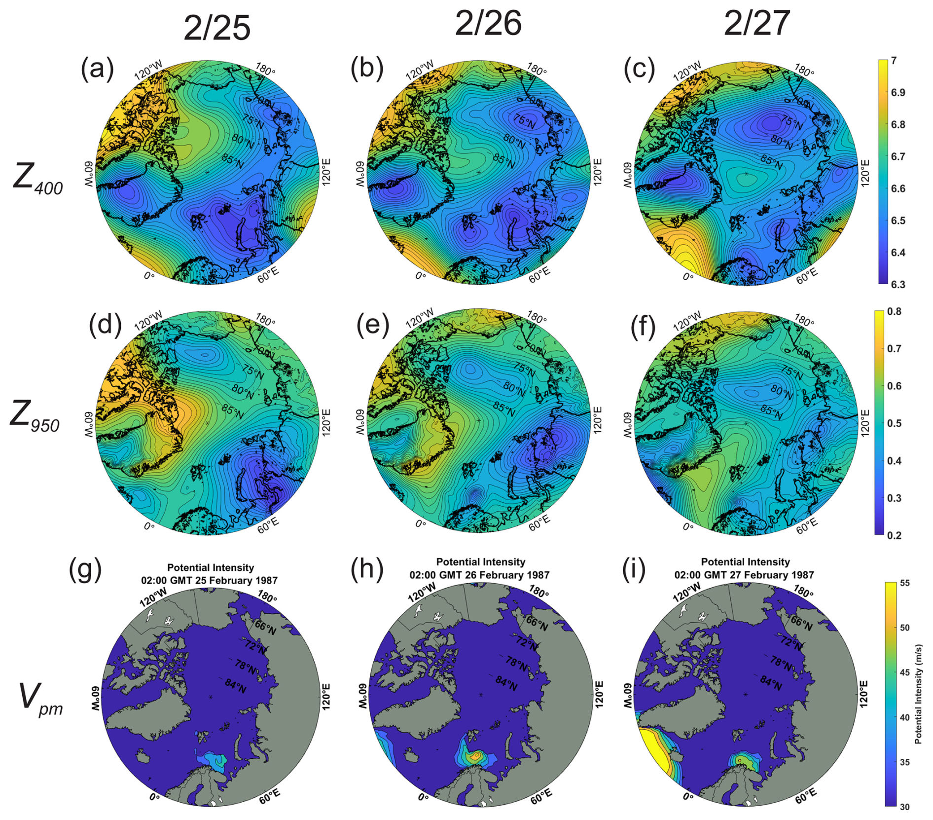
Figure 13 400 hPa geopotential height (km) at intervals of 23.3 m (a–c), 950 hPa geopotential height (km) in intervals of 20 m (d–f), and V_pm (m s⁻¹) in intervals of 4 m s⁻¹ (g–i), at 02:00 UTC on 25 February (left), 26 (center), and 27 (right), 1987. From ERA-5 reanalysis.

Figure 10 compares total column water retrieved from satellite microwave and near-infrared imagers (a) to that from the ERA5 reanalysis (b). While there is some broad agreement between the two estimates, the ERA5 underestimates column water in the critical region just east of Tunisia and overestimates it in an arc extending from eastern Sicily southeastward to the Libyan coast. Cyclop intensity, in analogy to tropical cyclone intensity, should be highly sensitive to low- and mid-level moisture in the mesoscale inner core region, which may be under-resolved and otherwise not well simulated by global NWP models. For this reason, we do not routinely show reanalysis of water vapor in this paper. The limitations of analyzed and forecast water vapor may constitute an important constraint on CYCLOP predictability and is a worthy subject for future research.

3.3 Polar low of February 1987

Closed upper tropospheric lows also provide favorable environments for CYCLOP development at very high latitudes in locations where there is open water. These usually form poleward of the mid-latitude jet, where quasi-balanced dynamics can be quite different from those operating at lower latitudes. Figure 11 is an infrared image of a polar low that formed just south of Svalbard on 25 February 1987, and tracked southward, making landfall on the north coast of Norway on 27 February. This system was studied extensively by Nordeng and Rasmussen (1992).

As with some medicanes, polar lows develop in strongly convecting air masses when cold air moves out over relatively warm water. The adjective “relatively” is crucial here; with polar lows the sea surface temperature is often only marginally above the freezing point of saltwater. Figure 12 shows the distribution of sea surface temperature on 25 February, with the uniform dark blue areas denoting regions of sea ice cover. The polar low shown in Fig. 11 develops when deep cold air moves southward over open water, as shown in Fig. 13.

In this case, it is not clear whether one can describe what happens in the upper troposphere (top row of Fig. 13) as a Rossby wave breaking event. Instead, what we see is a complex rearrangement of the tropospheric winter polar vortex, as a ridge building over North America breaks and forms an anticyclone over the North Pole. This complex rearrangement results in the formation of a deep cutoff low just south of Svalbard by 26 February, which then moves southward over Norway by 27 February. The polar low is barely visible in the 950 hPa height field on 25 February (middle row of Fig. 13), but intensifies rapidly as it moves over progressively warmer water, reaching maturity before landfall on 27 February.

The evolution of the V_pm field is shown in the bottom row of Fig. 13. The potential intensity increases rapidly south of Svalbard as the cut-off cyclone moves out over open water.

Under these conditions, most of the surface flux that drives the CYCLOP is in the form of sensible, rather than latent heat flux, and the background state has a nearly dry (rather than moist) adiabatic lapse rate. As shown by Cronin and Chavas (2019) and Velez-Pardo and Cronin (2023), surface flux-driven cyclones can develop in perfectly dry convecting environments, though they generally reach smaller fractions of their potential intensity and lack the long tail of the radial profile of azimuthal winds that is a consequence of the dry stratification resulting from background moist convection (Chavas and Emanuel, 2014). They also have larger eyes relative to their overall diameters. Given the low temperatures at which they occur, polar lows may be as close to the Cronin-Chavas dry limit as one might expect to see in Earth's climate.

One interesting feature of polar waters in winter is that the thermal stratification is sometimes reversed from normal, with warmer waters lying beneath cold surface waters. This is made possible, in part, by strong salinity stratification, that keeps the cold water from mixing with the warmer waters below. Therefore, it is possible for polar lows to generate warm, rather than cold, wakes, and this would feed back positively on their intensity. This seems to happen in roughly half the documented cases of polar lows in the Nordic seas (Tomita and Tanaka, 2024).

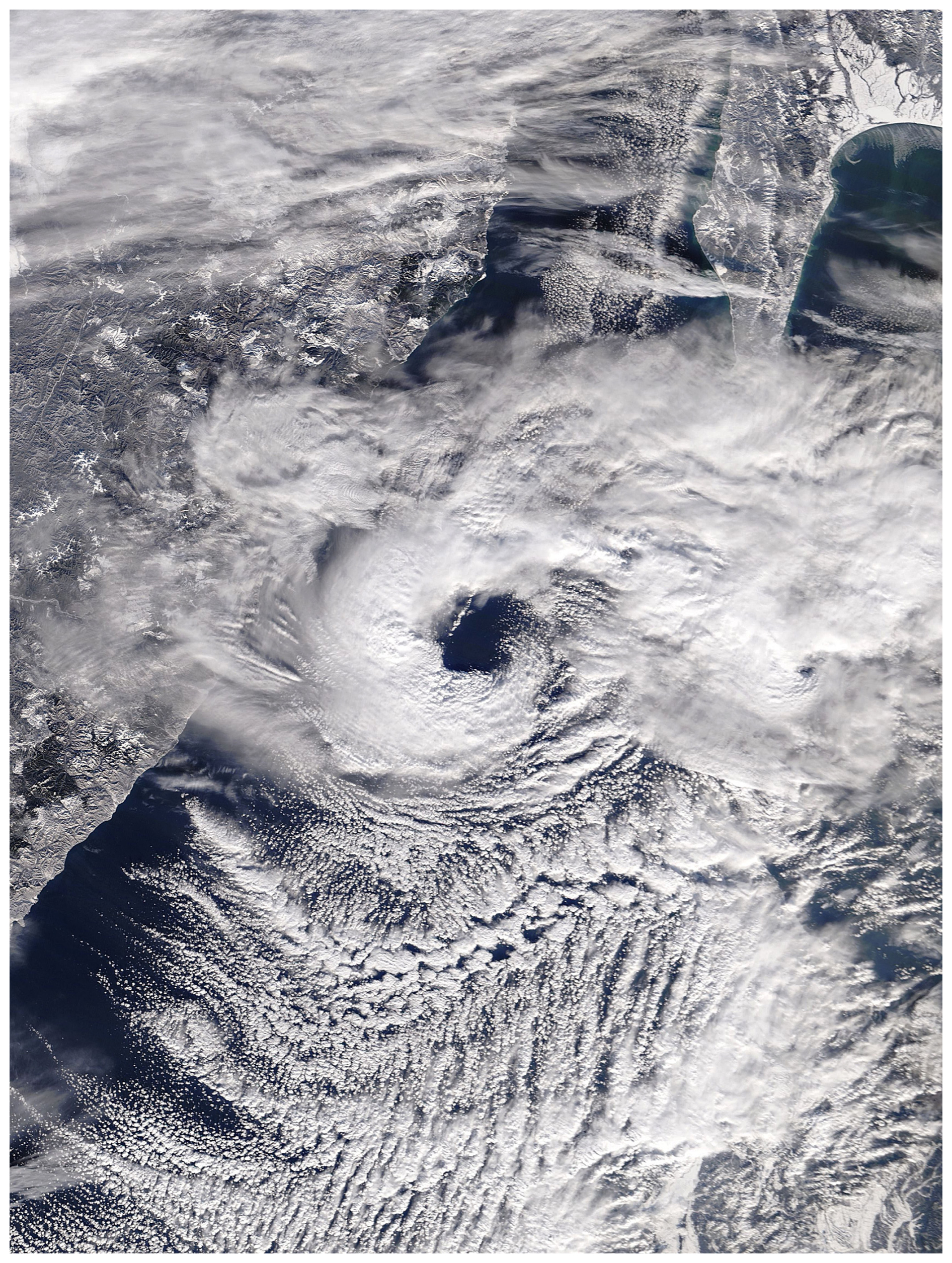
Figure 14 Polar low over the northern Sea of Japan, 02:13 UTC 20 December 2009 as captured by the MODIS imager on NASA's Terra satellite.

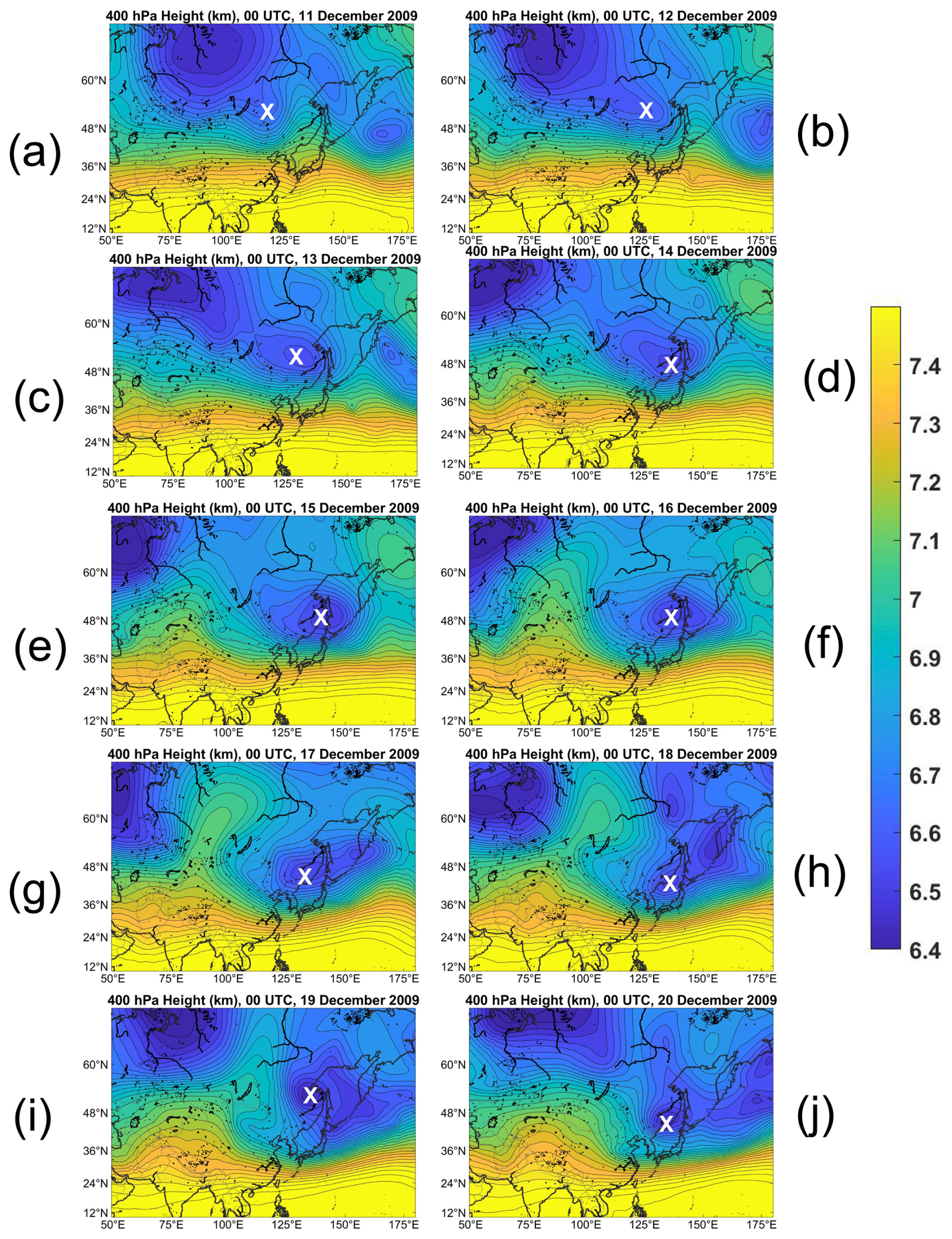
Figure 15 Sequence of 400 hPa geopotential height (km) charts at 1 d intervals from 00:00 UTC on 11 December (a) to 00:00 UTC on 20 December (j), 2009. The charts span from 0 to 180° longitude and from 10 to 70° latitude, and the contour increment is 36.7 m. The white crosses mark the center of the 400 hPa cyclone that was ultimately associated with the polar low. From ERA-5 reanalysis.

3.4 Polar low over the Sea of Japan, December 2009

Polar lows are not uncommon in the Sea of Japan, forming when deep, cold air masses from Eurasia flow out over the relatively warm ocean. They are frequent enough to warrant a climatology (Yanase et al., 2016). A satellite image of one such storm is shown in Fig. 14.

The cyclone traveled almost due south from this point, striking the Hokkaido region of Japan, near Sapporo, with gale-force winds and heavy snow. As with other CYCLOPs, it formed in an environment of deep convection under a cold low aloft.

The development of the cutoff cyclone aloft was complex, as shown by the sequence of 400 hPa maps displayed in Fig. 15. These are 00:00 UTC charts at 1 d intervals beginning on 11 December and ending on 20 December, about the time of the image in Fig. 14. A large polar vortex is centered in northern central Russia on 11 December but sheds a child low southeastward on 12 and 13 December, becoming almost completely cutoff on 14 December. The parent low drifts westward during this time. The newly formed cutoff cyclone meanders around in isolation from 15 December through 17 December, but becomes wrapped up with a system propagating into the domain from the east on 18 December. By 20 December, a small-scale cutoff cyclone is drifting southward over the northern Sea of Japan, and it is this upper cutoff that spawns the polar low.

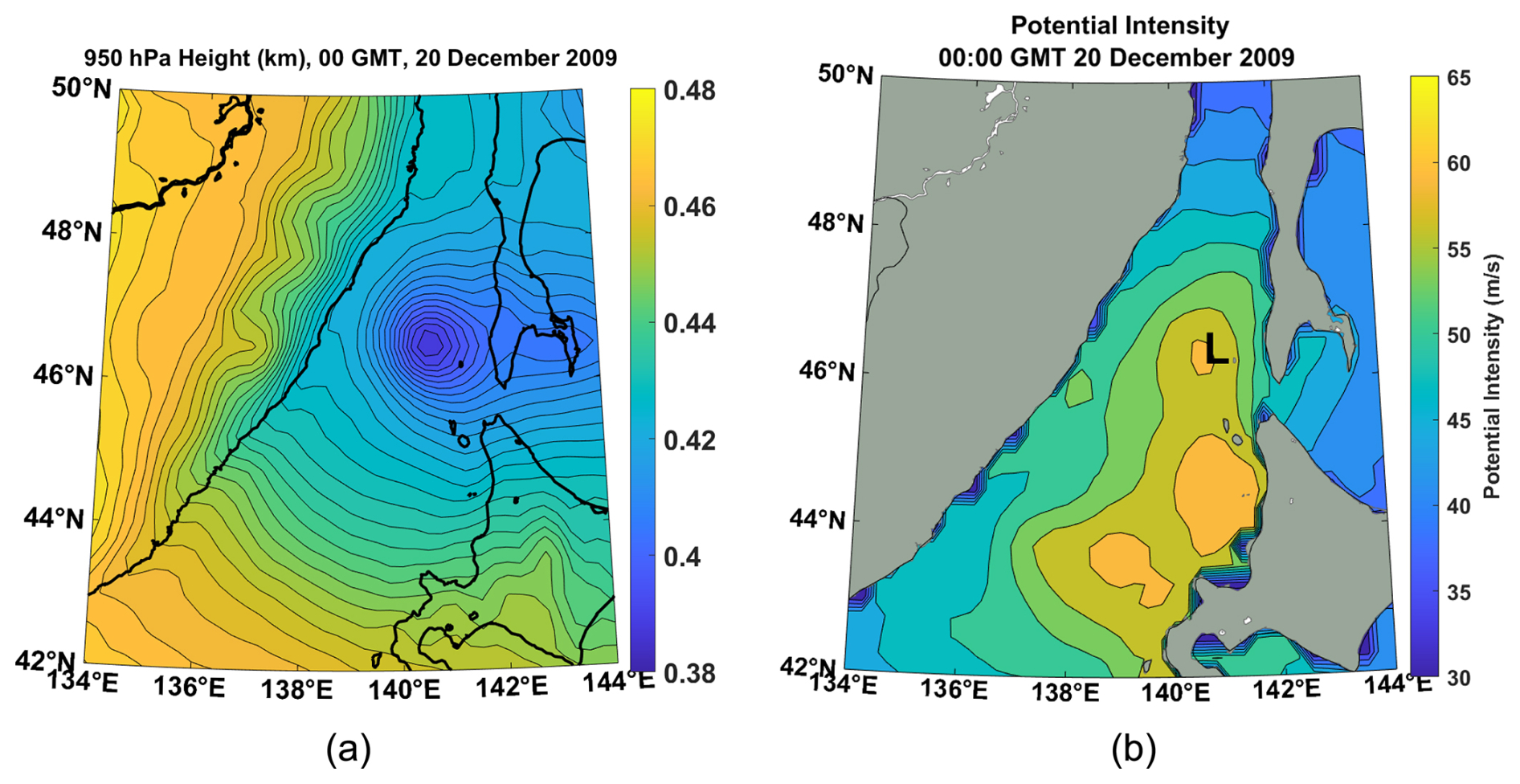
Figure 16 950 hPa geopotential height (a; km) at intervals of 3 m, and V_pm at intervals of 3 m s⁻¹ (b), at 00:00 UTC on 20 December 2009. In (b), the “L” marks the satellite-derived surface cyclone center. From ERA-5 reanalysis.

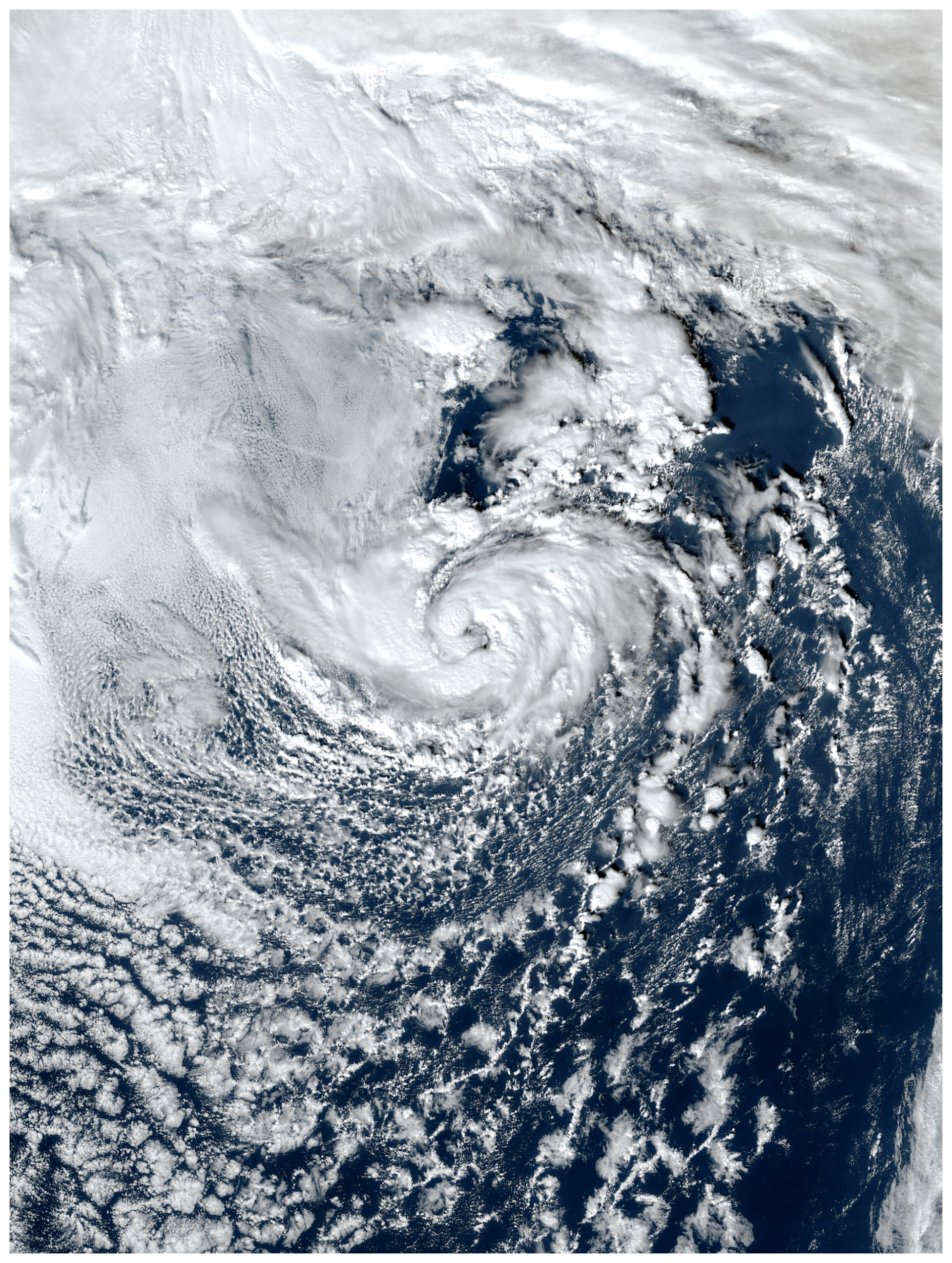
Figure 17 Subtropical cyclone over the western North Atlantic, 18:20 UTC, 16 January 2023. NOAA geostationary satellite image.

The 950 hPa height and the V_pm fields at 00:00 UTC on 20 December are shown in Fig. 16. At this time, the surface low is developing rapidly and moving southward into a region of high potential intensity. The latter reaches a maximum near the northwest coast of Japan, where the sea surface temperatures are larger. As with the two medicane cases and the other polar low case, the CYCLOP develops in a place where the potential intensity values are normally too low for surface flux-driven cyclones but for which the required potential intensity is created by the movement of a deep cold cyclone aloft over relatively warm water. The reanalysis 750 hPa temperature (not shown) presents a local maximum at the location of the surface cyclone at this time.

3.5 The subtropical cyclone of January 2023

The term “subtropical cyclone” has been used to describe a variety of surface flux-assisted cyclonic storms that do not strictly meet the definition of a tropical cyclone. The term has an official definition in the North Atlantic⁵ but is used occasionally elsewhere, especially in regions where terms like medicane, polar low, and Kona storm do not apply, such as the South Atlantic (Evans and Braun, 2012; Gozzo et al., 2014). Here we will use the term to designate CYCLOPs in the sub-arctic North Atlantic; that is, surface flux-powered cyclones that develop in regions and times whose climatological thermodynamic potential is small or zero, that would not be called polar lows owing to their latitude. This usage may not be consistent with other definitions. The point here is to show that CYCLOPs can occur in the North Atlantic and we can safely refer to these as CYCLOPs whether or not they meet some definition of “subtropical cyclone”.

Figure 17 displays a visible satellite image of a subtropical cyclone over the western North Atlantic on 16 January 2023. It resembles the medicanes and polar lows described previously, and like them, formed under a cutoff cyclone aloft.

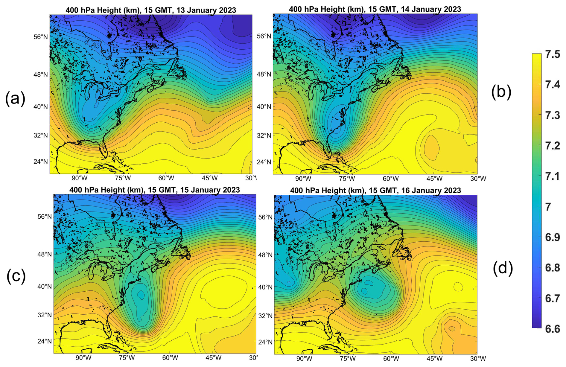
Figure 18 400 hPa geopotential height (km) at intervals of 30 m, at 15:00 UTC on 13 January (a), 14 January (b), 15 January (c), and 16 January (d), 2023. From ERA-5 reanalysis.

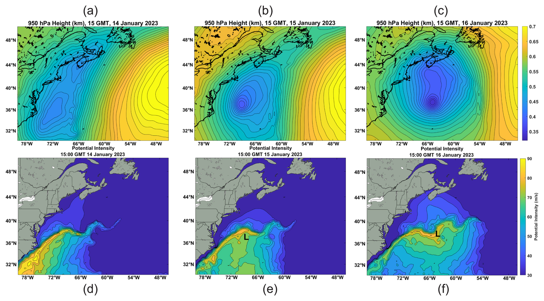
Figure 19 The 950 hPa geopotential height (km) at 15:00 UTC on 14 January (a), 15 (b), 16 (c); the V_pm field in increments of 5 ms⁻¹, on 14 January (d), 15 January (e), and 16 January (f). In (e) and (f) the “L” shows the position of the 950 hPa cyclone center at the time of the chart. From ERA-5 reanalysis.

The formation of the cutoff cyclone aloft is shown in Fig. 18. A deep trough advances slowly eastward over eastern North America and partially cuts off on 14 January. As the associated cold pool and region of light shear migrate out over the warm waters south of the Gulf Stream, a CYCLOP forms and intensifies with peak winds of around 60 kts at around 00:00 UTC on 17 January (Papin et al., 2023). Note also the anticyclonic wave breaking event to the east of the surface cyclone development, in the eastern half of panels 18b–d.

The evolutions of the 950 hPa and associated V_pm fields are displayed in Fig. 19. (Note the smaller scale around the developing surface cyclone, compared to Fig. 18.) On 14 January, the only appreciably large values of V_pm are associated with the Gulf Stream and in the far southwestern portion of the domain. The 950 hPa height field shows a broad trough associated with the baroclinic wave moving slowly eastward off the US east coast. But as the upper cold cyclone moves out over warmer water on 15 January, large V_pm south of the Gulf Stream, and a closed and more intense surface cyclone develops under the lowest 400 hPa heights and over the region with higher V_pm values.

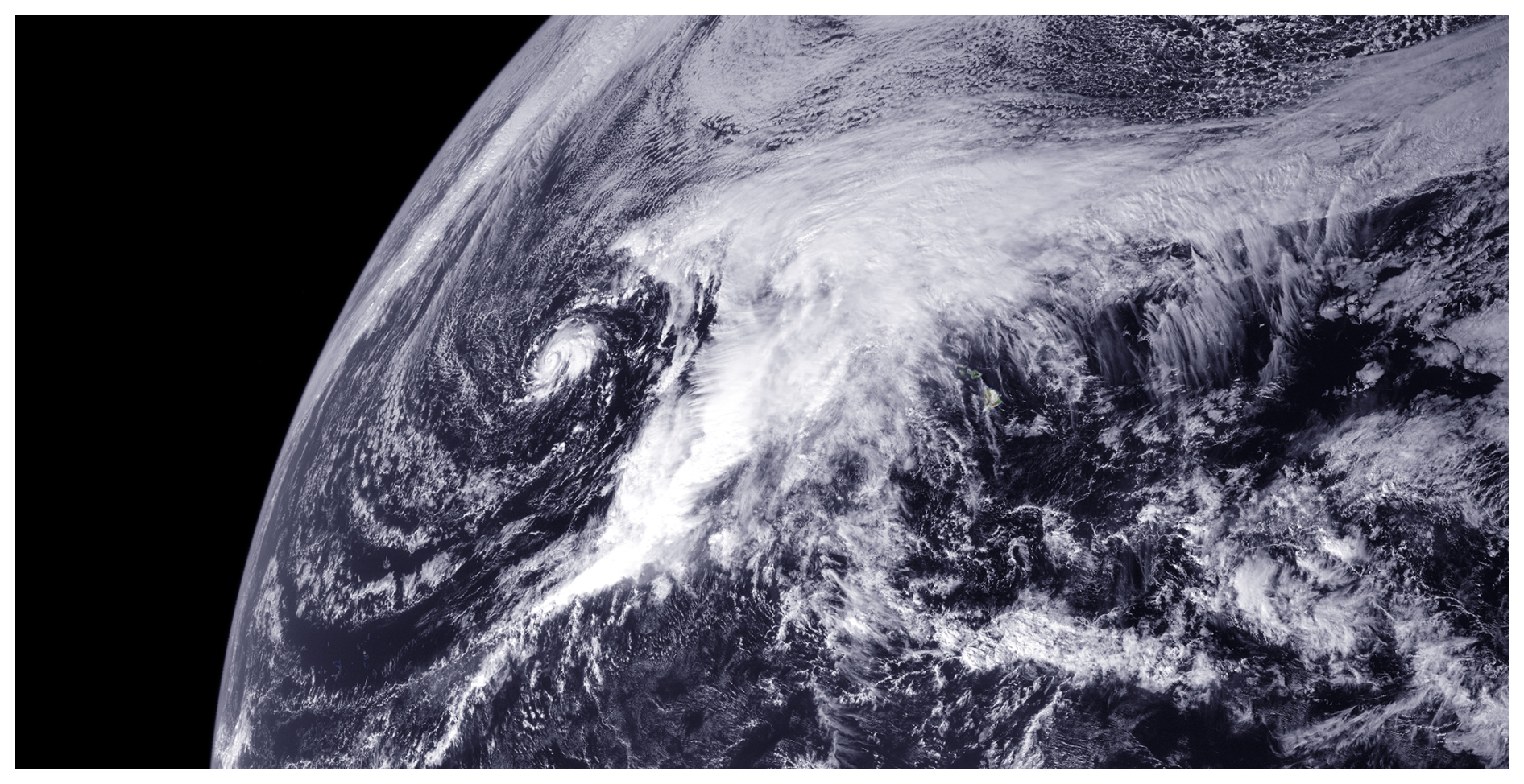
Figure 20 Geostationary satellite visible image showing a Kona Storm at 00:00 UTC on 19 December 2010. The Kona Storm is the small-scale cyclone left of the major cloud mass. (Image credit: NOAA-NASA GOES Project, image)

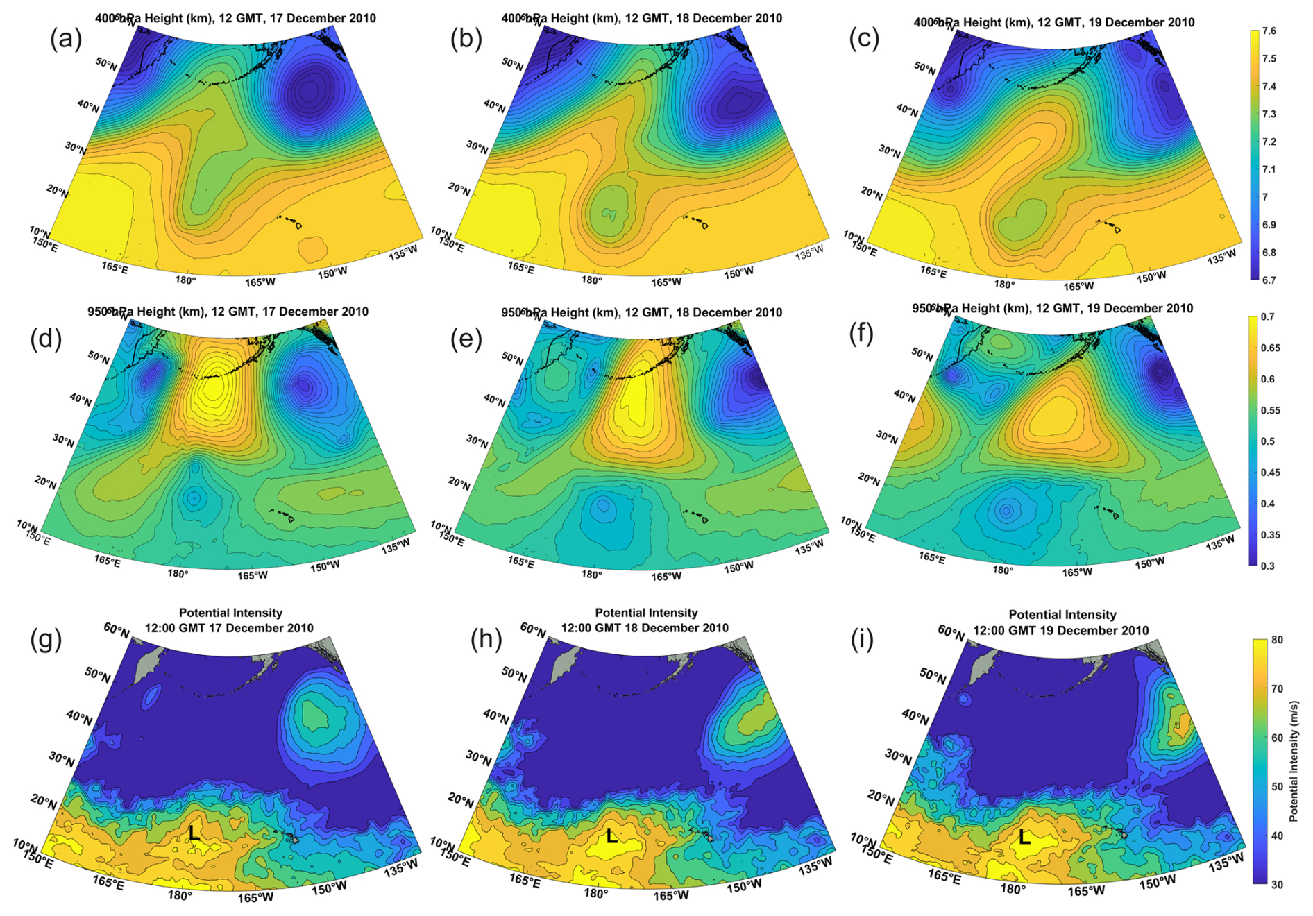
Figure 21 Sequence of 400 hPa geopotential height charts (km) at contour intervals of 30 m (a–c), 950 hPa geopotential heights (km) with contour intervals of 13.34 m (d–f), and V_pm contour intervals of 5 ms⁻¹ (g–i) at 12:00 UTC on 17 December (a, d, g), 18 December (b, e, h), and 19 December (c, f, i) 2010. The “L”s in (g)–(i) denote the positions of the 950 hPa cyclone center. From ERA-5 reanalysis.

As the upper tropospheric cyclone begins to pull out toward the northeast on 16 January, the surface cyclone intensifies in the region of large V_pm south of the Gulf Stream, while the more gradual warming of the surface air in the region of small V_pm north of the Stream yields surface pressure falls, but not as concentrated and intense as in the CYCLOP to the south.

Although the evolution of the upper tropospheric cyclone differs in detail from the previously examined cases, and the sharp gradient of sea surface temperature across the north wall of the Gulf Stream clearly plays a role here, in other respects the development of this subtropical cyclone resembles that of other CYCLOPs, developing in regions of substantial thermodynamic potential that result, at least in part, from cooling aloft on synoptic time and space scales.

3.6 A Kona Storm

Hawaiians use the term “Kona Storm” to describe cold-season storms that typically form west of Hawaii and often bring damaging winds and heavy rain to the islands. The term “Kona” translates to “leeward”, which in this region means the west side of the islands. They may have been first described in the scientific literature by Daingerfield (1921). Simpson (1952) states that Kona Storms possess “cold-core characteristics, with winds and rainfall amounts increasing with distance from the low-pressure center and reaching a maxima at a radius of 200 to 500 mi. However, with intensification, this cyclone may develop warm-core properties, with rainfall and wind profiles bearing a marked resemblance to those of the tropical cyclone”. In general, Simpson's descriptions of the later stages of some Kona Storms are consistent with their being CYCLOPs. But it should be noted that the term is routinely applied to cold-season storms that bring hazardous conditions to Hawaii regardless of whether they have developed warm cores. A good review of the climatology of Kona storms is provided by Otkin and Martin (2004), who state that “development of the surface cyclone in all types results from the intrusion of an upper-level disturbance of extratropical origin into the subtropics”. Here we focus on Kona storms that do develop warm cores, providing as a first example the Kona Storm of 19 December 2010. A visible satellite image of this storm is shown in Fig. 20.

As with all known CYCLOPs, the December 2010 Kona Storm developed under a cold-core cutoff cyclone aloft, as shown in Fig. 21. The upper-level cyclone had a long and illustrious history before 18 December, having meandered over a large swath of the central North Pacific. But beginning on 7 December, the cutoff cyclone made a decisive swing southward over waters with higher values of V_pm. A broad surface cyclone was present underneath the cold pool aloft on all three days, but developed a tight inner core on 19 December as the cold pool slowly drifted over a region of higher potential intensity.

This Kona Storm developed in a region of modest climatological potential intensity that was, however, substantially enhanced by the cutoff cyclone aloft. For example, on 17 December, the conventional (unmodified) potential intensity at the position of the 950 hPa cyclone center was about 55 ms⁻¹, compared to the 75–80 ms⁻¹ values of the modified potential intensity. One can only speculate whether a surface flux-driven cyclone would have developed without the enhanced cooling associated with the cutoff cyclone aloft.

This Kona storm was identified as a tropical storm by the Central Pacific Hurricane Center, as of 09:00 UTC 20 December, and given the name Omeka.

The Kona Storm of March 1951 is a more unambiguous case of a CYCLOP. Figure 22 shows the 950 hPa geopotential height field on 26 March 1951. The storm, at that time, was classified by the Joint Typhoon Warning Center as a tropical cyclone, but the climatological potential intensity there at that time of year could not have supported any tropical cyclone. Figure 22c shows that substantial V_pm was associated with a cutoff cyclone in the upper troposphere, making possible the existence of this CYCLOP.

4 Variations on the Theme

We here are attempting to distinguish a class of cyclones, CYCLOPs, from other cyclonic storms by the physics of their development, not by the regions in which they develop. Here we present a case of an actual tropical cyclone in the Mediterranean that we do not identify as a CYCLOP.

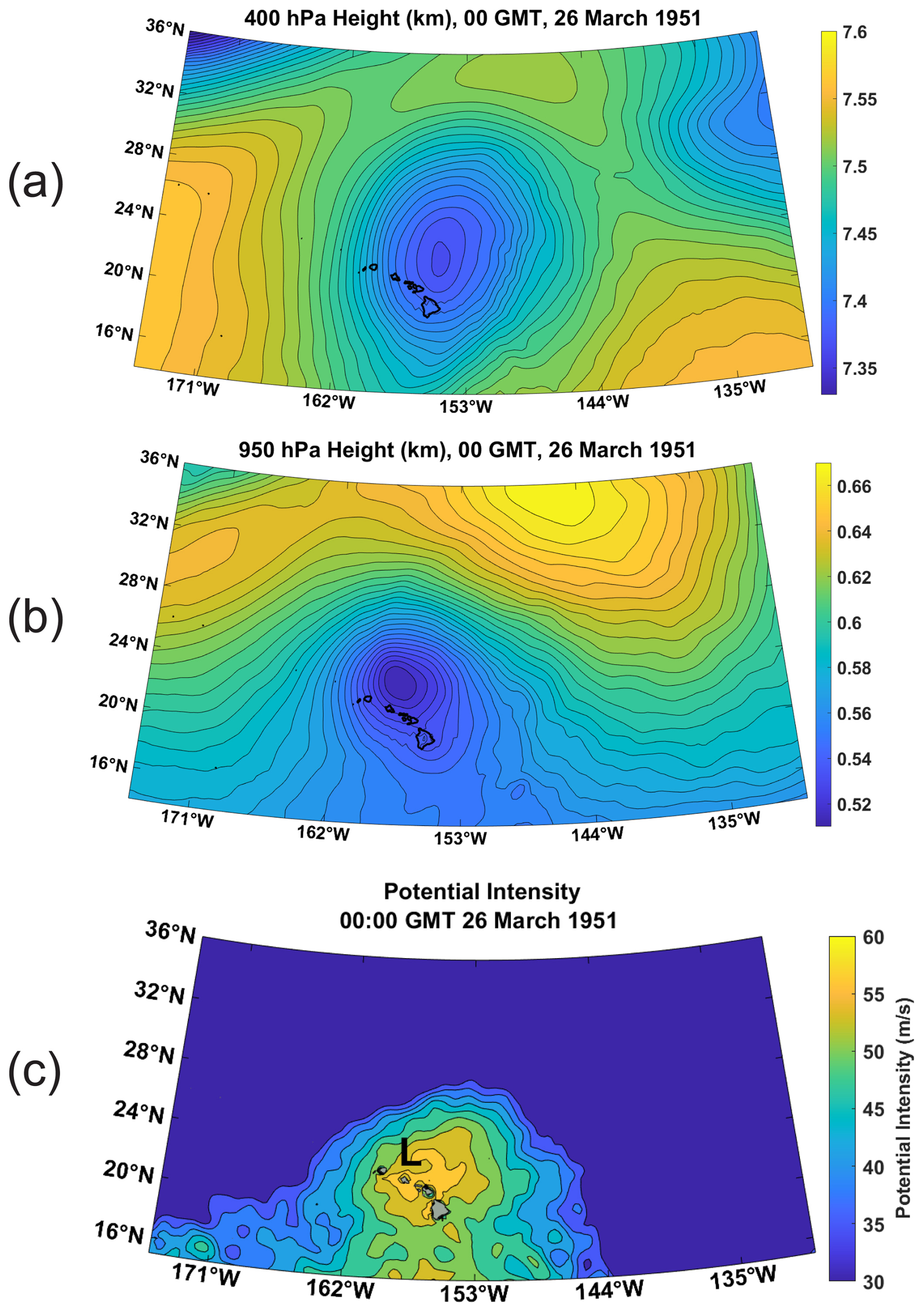
Figure 22 Kona Cyclone of March 1951. Fields are shown at 00:00 UTC on 26 March: (a) 400 hPa geopotential height (km) with a 10 m contour interval, (b) 950 hPa geopotential height (km) with 5 m contour interval, and (c) V_pm with a contour interval of 3 ms⁻¹.

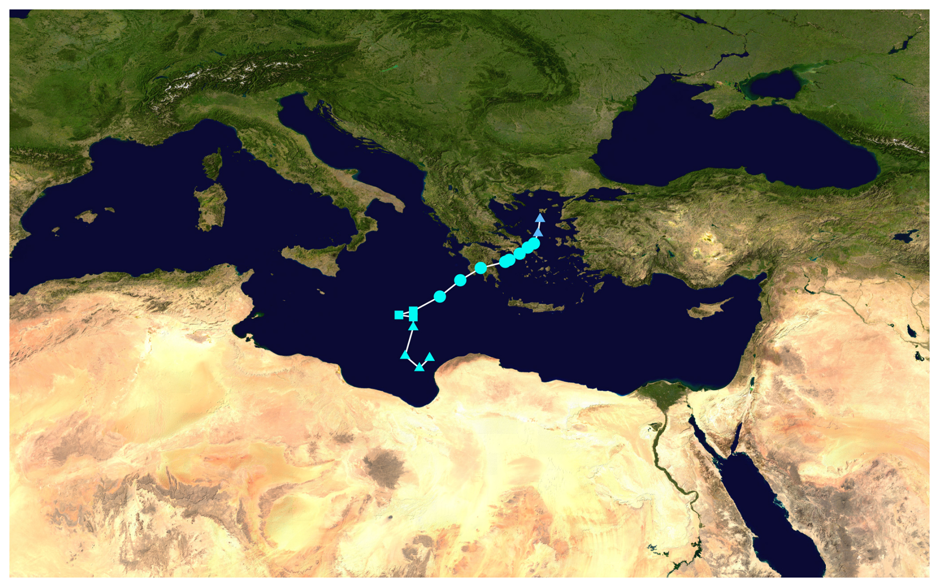
Figure 23 Track of Cyclone Zorbas, from 27 September through 2 October 2018. (Image credit: Wikipedia Commons; https://commons.wikimedia.org/wiki/File:Zorbas_2018_track.png, last access: 15 June 2025).

4.1 Cyclone Zorbas

The cyclone known as Zorbas developed just north of Libya on 27 September 2018 and moved northward and then northeastward across the Peloponnese and the Aegean (Fig. 23), dissipating in early October. The storm killed several people and did millions of dollars of damage.

The antecedent (actual, not modified) potential intensity distribution, on 26 September, is displayed in Fig. 24. In much of the southern part of the central Mediterranean, the potential intensity was typical of tropical warm pools with values approaching 80 ms⁻¹. As with most medicanes, Zorbas was triggered by an upper tropospheric Rossby wave breaking event (Fig. 25), but in this case the cold pool aloft only enhanced the existing potential intensity by about 7 ms⁻¹ (on 27 September). In this case, the maximum 400 hPa geopotential perturbation was around 1500 m² s⁻², compared to about 2500 m² s⁻² in the case of Medicane Zeo of 2005. Zorbas was therefore more like a classic case of a tropical cyclone resulting from tropical transition (Bosart and Bartlo, 1991; Davis and Bosart, 2003, 2004) and we might not describe it as a CYCLOP. Note that while the approach of the upper-level cyclone did not appreciably alter the potential intensity, it almost certainly humidified the middle troposphere, making genesis somewhat more likely, as may be true in most cases of tropical transition.

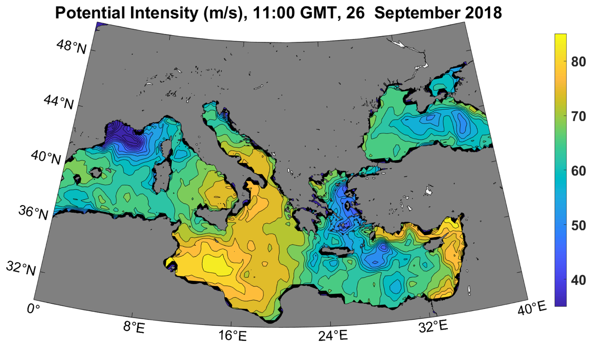
Figure 24 Actual potential intensity distribution in the Mediterranean and Black Seas, 11:00 UTC on 26 September 2018.

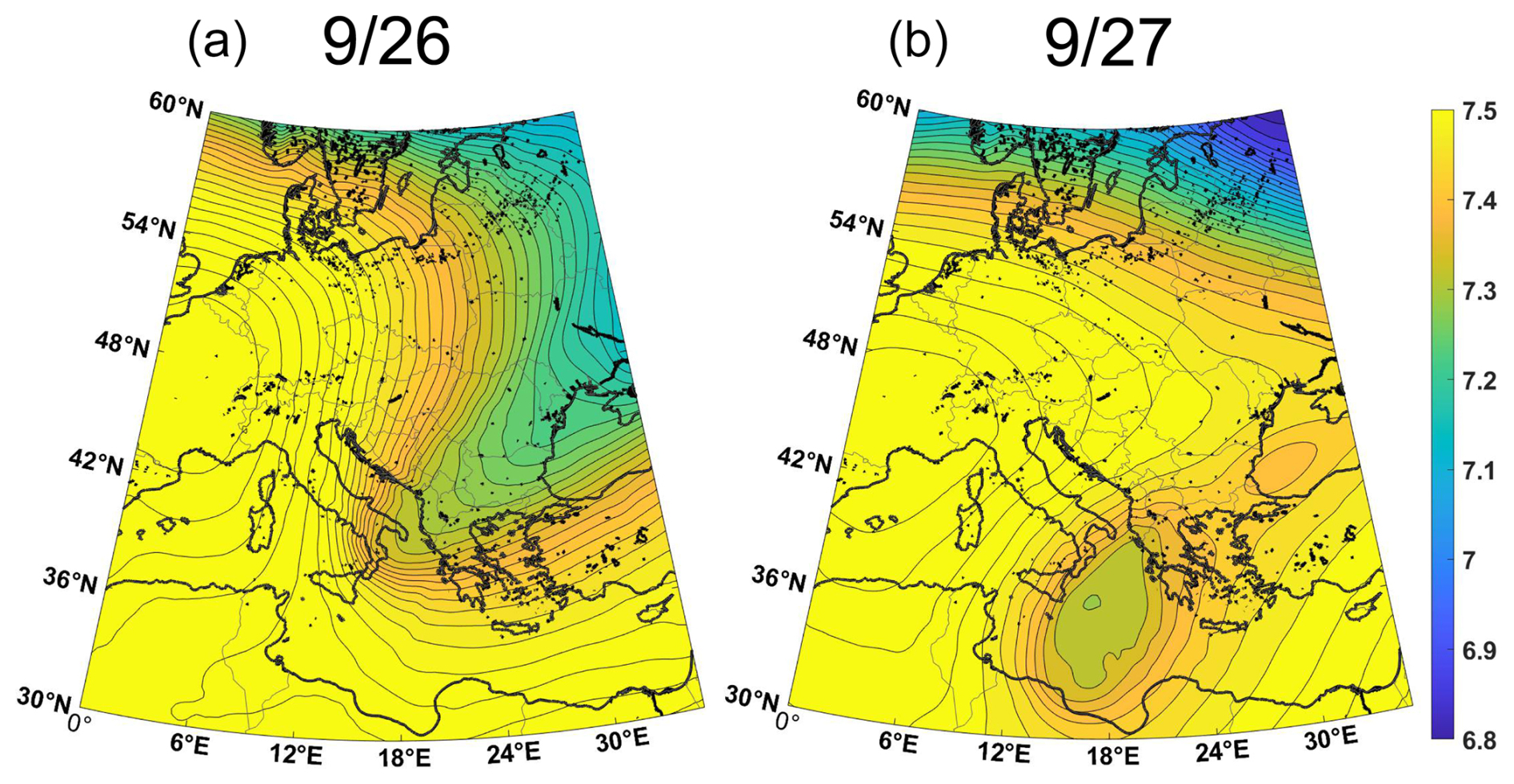
Figure 25 400 hPa geopotential height (km) at 11:00 UTC on 26 September (a) and 27 September (b), 2018. Contour interval is 13.34 m. From ERA-5 reanalysis.

4.2 Cyclone Daniel

Cyclone Daniel of 2023 was the deadliest Mediterranean surface flux-driven cyclone in recorded history, with a death toll exceeding 4000 and thousands of missing persons, mostly owing to floods caused by the catastrophic failure of two dams near Derna, Libya (Flaounas et al., 2024). This flooding was the worst in the recorded history of the African continent. Figure 26 shows the track of Daniel's center and a visible satellite image of the storm as it approached landfall in Libya is shown in Fig. 27. Daniel became a surface flux-driven cyclone off the west coast of the Peloponnese on 5 September, made landfall near Benghazi, Libya, on 10 September and dissipated over Egypt on 12 September.

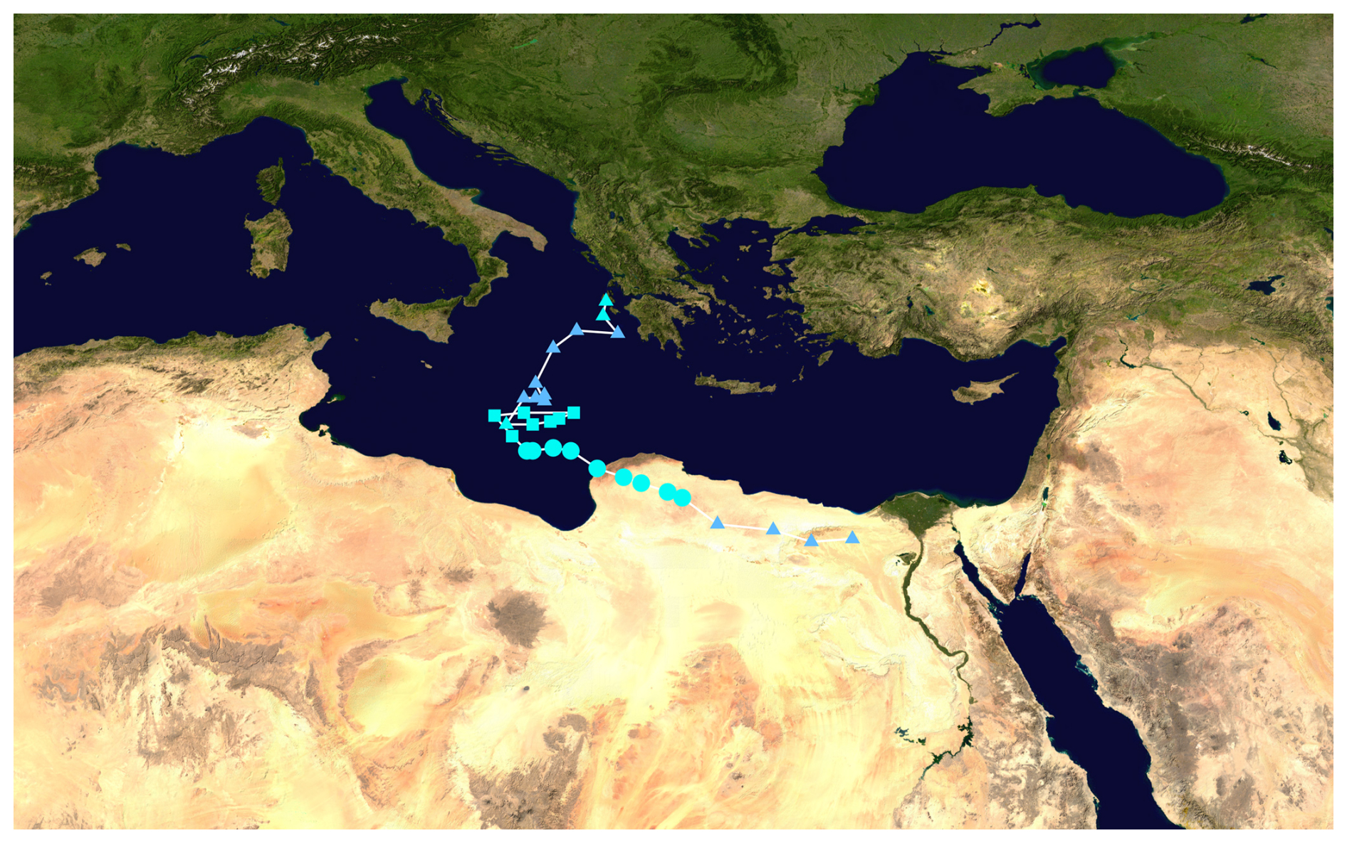
Figure 26 Track of Storm Daniel at 6 h intervals, beginning 5 September and ending 12 September 2023. The circles, squares and triangles along the track denote tropical cyclone, subtropical cyclone and extratropical cyclone designations, respectively, while the deep blue and light blue colors denote tropical depression- and tropical storm-force winds. (Image credit: Wikipedia commons; https://commons.wikimedia.org/wiki/File:Daniel_2023_track.png, last access: 16 June 2025)

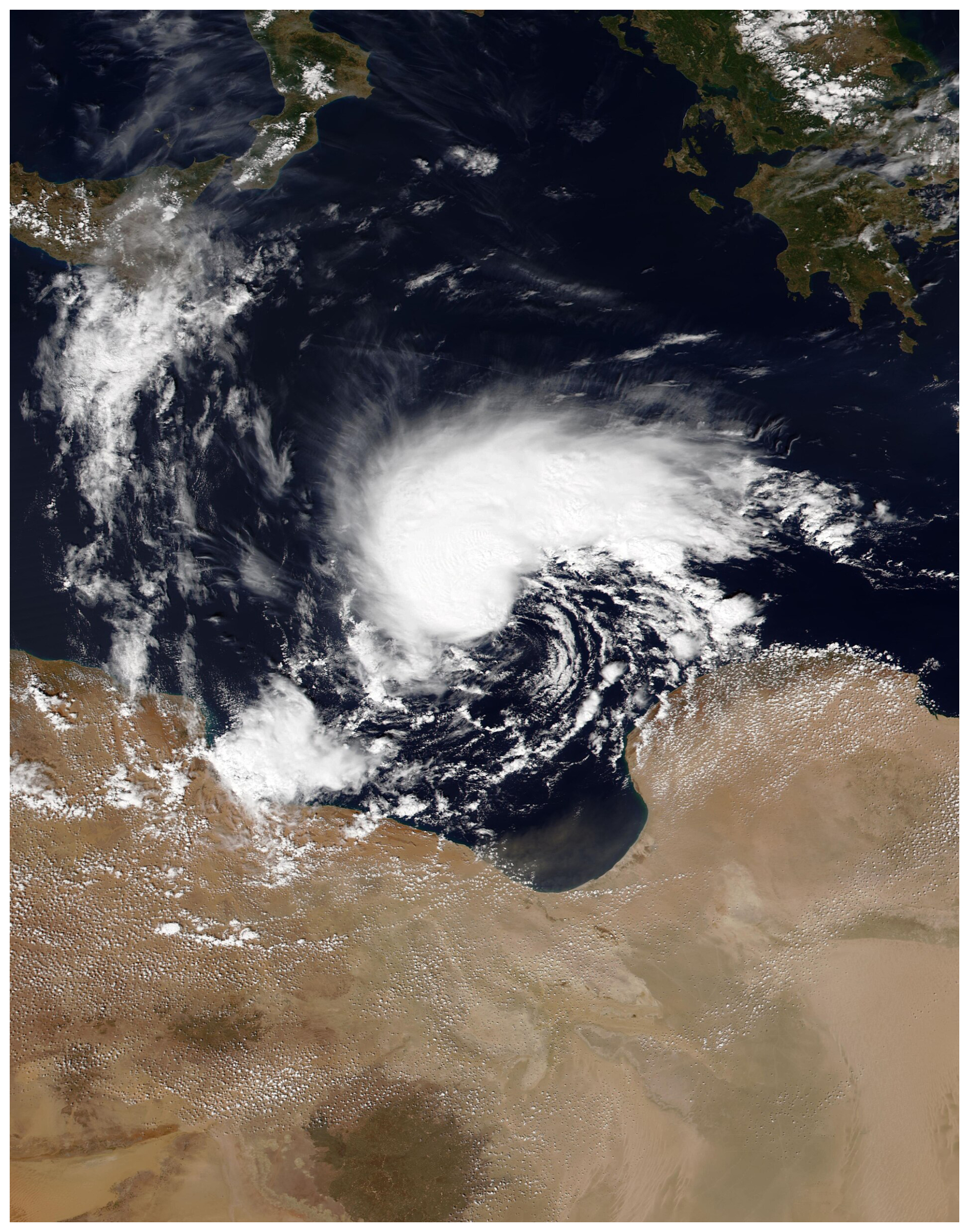
Figure 27 NOAA-20 VIIRS image of Storm Daniel at 12:00 UTC 9 September 2023, as it approached the Libyan coast.

As with Zorbas, the antecedent potential intensity was high throughout the Mediterranean south and east of Italy and Sicily, and the event was triggered by a Rossby wave breaking event (Fig. 28). And as with Zorbas, the cutoff cyclone aloft was not strong enough to appreciably alter the existing potential intensity but acted as a trigger for the tropical cyclone that Daniel became. This was another classic case of tropical transition, and not a CYCLOP.

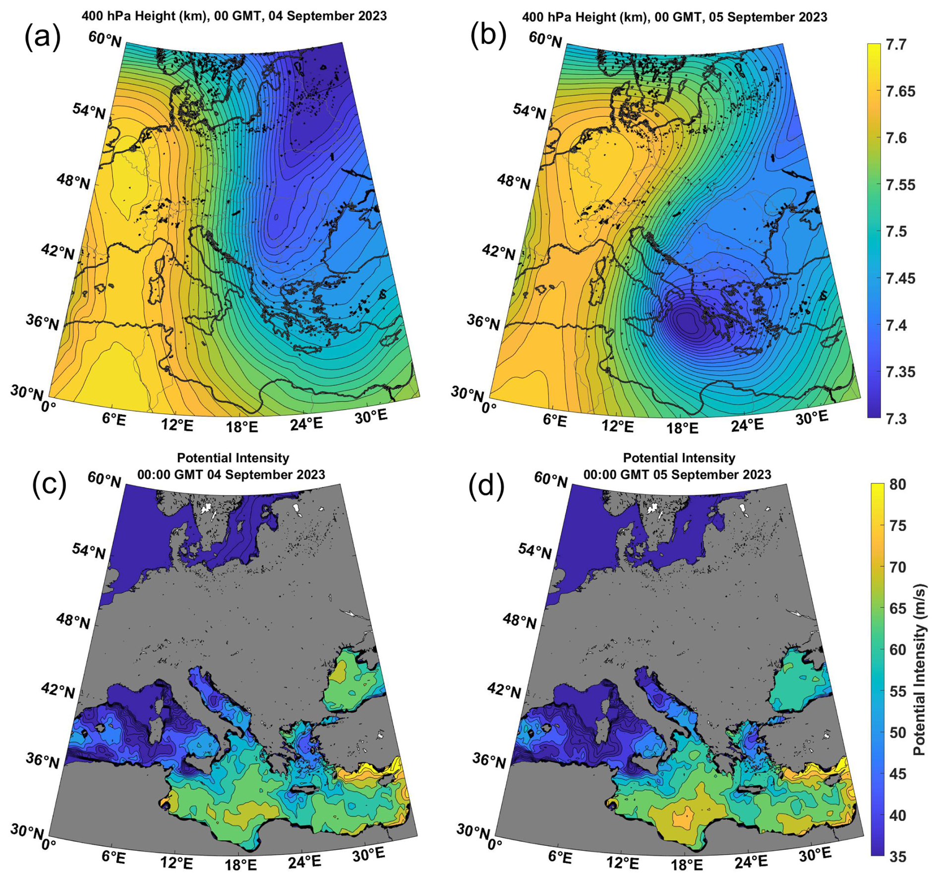
Figure 28 400 hPa geopotential height (km) with contour interval of 13.33 m (a–b); and actual potential intensity (ms⁻¹) with contour interval of 4 ms⁻¹ (c–d) at 00:00 UTC 4 September (a, c) and 5 September (b,d), from ERA-5 reanalyses.

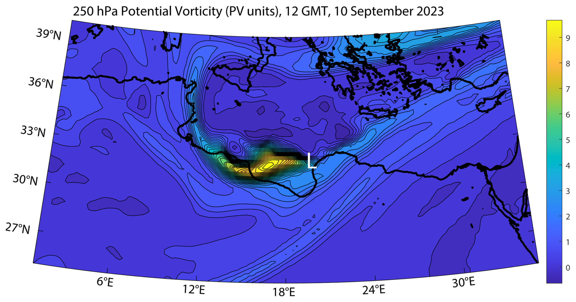
Figure 29 Potential vorticity (PV units, 10⁻⁶ K kg⁻¹ m² s⁻¹) at 250 hPa at 12:00 UTC on 10 September 2023. The white “L” marks the approximate surface center of Daniel at this time.

Yet Storm Daniel differed from Zorbas in one important respect: as it approached the Libyan coast around 10 September, it came under the influence of strong high-level potential vorticity (PV) advection owing to a mesoscale “satellite” PV mass rotating around the upper-level cutoff cyclone (Fig. 29). The quasi-balanced forcing associated with the superposition of the high-level PV anomaly with the surface-based warm core probably contributed to Daniel's intensification which, remarkably for a surface flux-driven cyclone, continued after landfall (Hewson et al., 2024).

5 Summary and conclusions

We here argue that many of the cyclonic storms called medicanes, polar lows, subtropical cyclones, and Kona storms operate on the same physics and ought to be identified as a single class of storms that we propose to call CYCLOPs. In their developed structure and intensity they are essentially identical to tropical cyclones, and like TCs are driven primarily by wind-dependent surface enthalpy (latent and sensible heat) fluxes, but unlike classical TCs, there is little or no climatological potential intensity for the storms. Rather, the development and/or migration over relatively warm water of strong, cold-core cyclones in the upper troposphere cools and moistens the column through dynamical lifting, generating mesoscale to synoptic scale columns with elevated potential intensity and humidity, and reduced wind shear – ideal embryos for the development of surface flux-driven cyclones.

We do not expect CYCLOPs to last as long as classical TCs. In the first place, the conditions that enable such storms are confined in space and transient in time. For example, the cutoff cyclone aloft is often re-absorbed into the main baroclinic flow. In addition, the strong surface enthalpy fluxes that power CYCLOPs also increase, through the action of deep convection, the enthalpy of the otherwise spatially limited cold columns in which they form, reducing over time the thermodynamic disequilibrium between the air column and the sea surface. A back-of-the-envelope estimate for the time to destroy the initial thermodynamic disequilibrium is on the order of days. By contrast, even the strongest classical TCs do not sufficiently warm the large expanses of the tropical troposphere they influence to appreciably diminish the large-scale potential intensity of tropical warm pools.

Not all cyclonic storms that have been called polar lows, medicanes, subtropical cyclones, or Kona storms meet our definition of CYCLOP. The literature describes many polar lows that have been traced to something more nearly like classical baroclinic instability acting in an air mass of anomalously low static stability (e.g. Sardie and Warner, 1985). Many storms identified as Kona storms because of their location and season, and which developed under cold cyclones aloft, never received much of a boost from surface fluxes and therefore would not be classified as CYCLOPs. And, as we described in the last section, two strong Mediterranean cyclones, Zorbas of 2018 and Daniel of 2023, developed in environments of high climatological potential intensity and formed via the tropical transition process.

Beyond these caveats, not all cold-core, closed cyclones in the upper troposphere that develop or move over relatively warm ocean waters develop CYCLOPs. Without doing a comprehensive survey, we have found several cases of greatly enhanced potential intensity under cold lows aloft that did not develop strong, concentrated surface cyclones. We suspect that, as with classical tropical cyclones, dry air incursions above the boundary layer may have prevented genesis in these cases, but as these events generally occur in regions devoid of in-situ observations, it is not clear how well reanalyses capture variations of moisture on the scale of CYCLOPs. In any event, the efficiency with which upper-level cut-off cyclones produce CYCLOPs, given a substantial perturbation in potential intensity, should be a subject of future research.

Clearly, there exists a continuum between pure tropical transition, in which synoptic-scale dynamics play no role in setting up the potential intensity, and pure CYCLOPs in which synoptic-scale processes create all the potential intensity that drives the storm. The distinction we are making here does not pertain to the final result – a tropical cyclone⁶ – but to the route to creating it. As a practical matter, forecasters should consider both the triggering potential and mesoscale to synoptic scale environmental development in predicting the formation and evolution of CYCLOPs. The modified potential intensity (V_pm) introduced here may prove to be a valuable diagnostic that can easily be calculated from NWP model output. To simulate CYCLOPs, NWP models need to make accurate forecasts of dynamic processes that lead to the formation and humidification of deep cold pools aloft, and be able to handle surface fluxes and other boundary layer processes essential to the formation of surface flux-driven cyclones. And, as with tropical cyclones, coupling to the ocean is essential for accurate intensity prediction.

Finally, we encourage researchers to focus on the essential physics of CYCLOP development regardless of where in the world they occur. Casting a broader geographical net will harvest a greater sample of such storms and should lead to more rapid progress in understanding and forecasting them.

Appendix A

CYCLOPs form when dynamical processes create synoptic-scale cold columns marked by cutoff cyclones in the upper troposphere. The objective here is to calculate tropical cyclone potential intensity in these cold columns. The problem is that the CYCLOPs themselves, and surface heat fluxes in general, warm the columns, sometimes rapidly, diminishing the potential intensity. We want to know what the potential intensity was before this warming occurs. Here we develop a modified potential intensity using the surface pressure depression as proxy for the column heating.

Potential intensity is a measure of the maximum surface wind speed that can be achieved by a cyclone fueled entirely by surface enthalpy fluxes. It is defined (see Rousseau-Rizzi and Emanuel, 2019 for an up-to-date definition):

$$\begin{array}{}\text{(A1)}& V_{\mathrm{p}}^{\mathrm{2}}={\displaystyle \frac{C_k}{C_{\mathrm{D}}}}{\displaystyle \frac{T_{\mathrm{s}}-T_{\mathrm{o}}}{T_{\mathrm{o}}}}\left(h_{\mathrm{0}}^{\ast }-h_{\mathrm{b}}\right),\end{array}$$

where C_k and C_D are the surface exchange coefficients for enthalpy and momentum, T_s and T_o are the absolute temperatures of the surface and outflow layer, $h_{\mathrm{0}}^{\ast }$ is the saturation moist static energy of the sea surface, and h_b is the moist static energy of the boundary layer.

Using the relation Tδs≃δh, where s is moist entropy, we can re-write Eq. (A1) slightly as

$$\begin{array}{}\text{(A2)}& V_{\mathrm{p}}^{\mathrm{2}}={\displaystyle \frac{C_k}{C_{\mathrm{D}}}}{\displaystyle \frac{T_{\mathrm{s}}-T_{\mathrm{o}}}{T_{\mathrm{o}}}}{T}_{\mathrm{s}}\left(s_{\mathrm{0}}^{\ast }-s_b\right).\end{array}$$

Next, we assume that the troposphere near CYCLOPs has a nearly moist adiabatic lapse rate⁷, and the moist entropy of the boundary layer is equal to the saturation moist entropy, $s^{\ast },$ of the troposphere; i.e., that the troposphere is neutrally stable to moist adiabatic ascent from the boundary layer. Under these conditions, Eq. (A2) may be re-written

$$\begin{array}{}\text{(A3)}& V_{\mathrm{p}}^{\mathrm{2}}={\displaystyle \frac{C_k}{C_{\mathrm{D}}}}{\displaystyle \frac{T_{\mathrm{s}}-T_{\mathrm{o}}}{T_{\mathrm{o}}}}{T}_{\mathrm{s}}\left(s_{\mathrm{0}}^{\ast }-s^{\ast }\right).\end{array}$$

Here s^∗ is constant with altitude, since the troposphere is assumed to have a moist adiabatic lapse rate.

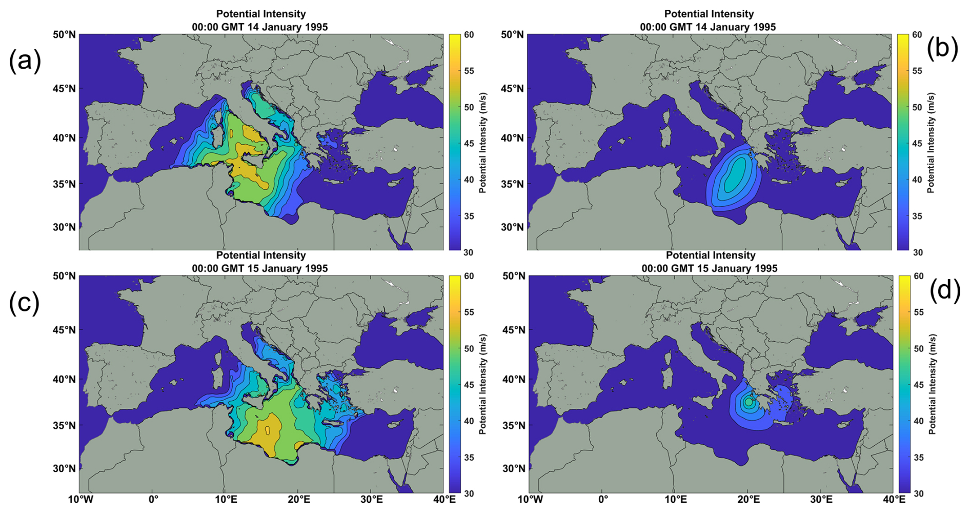
Figure A1 Unmodified potential intensity (a, c) and modification of the potential intensity (b, d) at 00:00 UTC on 14 January (a, b) and 15 January (c, d). Note that the full modified potential intensity is not the arithmetic sum of these two contributions but rather their Euclidean norm.

Referring to Fig. 1a in the main text, we want to know what the potential intensity is in the vicinity of the cutoff cyclone aloft before the atmosphere underneath it has started to warm up under the influence of surface enthalpy fluxes. But in reality, this warming commences as soon as the system moves over relatively warm water and deep convection begins. We can estimate what the temperature, or s^∗, was before the warming began by using the surface pressure drop as a proxy for the column warming.

We begin with the perturbation hydrostatic equation in pressure coordinates:

$$\begin{array}{}\text{(A4)}& {\displaystyle \frac{\partial {\mathit{\varphi }}^{\prime }}{\partial p}}=-{\mathit{\alpha }}^{\prime },\end{array}$$

where ϕ^′ is the perturbation geopotential and α^′ is the perturbation specific volume. Since the latter is a function of pressure and s^∗ only, we can use the chain rule and one of the Maxwell relations from thermodynamics (Emanuel, 1994) to write Eq. (A4) as

$$\begin{array}{}\text{(A5)}& {\displaystyle \frac{\partial {\mathit{\varphi }}^{\prime }}{\partial p}}=-{\left({\displaystyle \frac{\partial T}{\partial p}}\right)}_{s\ast }s{\ast }^{\prime }.\end{array}$$

Now, since $s{\ast }^{\prime }$ does not vary with altitude, we can integrate Eq. (A5) from the surface to the local tropopause to yield

$$\begin{array}{}\text{(A6)}& -{\mathit{\varphi }}_{\mathrm{s}}^{\prime }=\left(T_{\mathrm{s}}-T_{{\mathit{\varphi }}^{\prime }=\mathrm{0}}\right)s{\ast }^{\prime }.\end{array}$$

where ${\mathit{\varphi }}_{\mathrm{s}}^{\prime }$ is the near-surface geopotential perturbation and $T_{{\mathit{\varphi }}^{\prime }=\mathrm{0}}$ is the absolute temperature at the level where the CYCLOP-induced geopotential perturbation vanishes.

Therefore the CYCLOP-induced warming of the troposphere is estimated as

$$\begin{array}{}\text{(A7)}& s{\ast }^{\prime }={\displaystyle \frac{-{\mathit{\varphi }}_{\mathrm{s}}^{\prime }}{T_{\mathrm{s}}-T_{{\mathit{\varphi }}^{\prime }=\mathrm{0}}}}.\end{array}$$

We subtract this warming from the reanalysis environmental saturation entropy in Eq. (A3), yielding

$$\begin{array}{}\text{(A8)}& V_{\mathrm{pm}}^{\mathrm{2}}={\displaystyle \frac{C_k}{C_{\mathrm{D}}}}{\displaystyle \frac{T_{\mathrm{s}}-T_{\mathrm{o}}}{T_{\mathrm{o}}}}{T}_{\mathrm{s}}\left(s_{\mathrm{0}}^{\ast }-s_{\mathrm{e}}^{\ast }-{\displaystyle \frac{{\mathit{\varphi }}_{\mathrm{s}}^{\prime }}{T_{\mathrm{s}}-T_{{\mathit{\varphi }}^{\prime }=\mathrm{0}}}}\right),\end{array}$$

where s_e∗ is the analyzed saturation entropy of the column. This can be written alternatively as

$$\begin{array}{}\text{(A9)}& V_{\mathrm{pm}}^{\mathrm{2}}=V_{\mathrm{p}}^{\mathrm{2}}-{\displaystyle \frac{C_k}{C_{\mathrm{D}}}}{\displaystyle \frac{T_{\mathrm{s}}}{T_{\mathrm{o}}}}{\displaystyle \frac{T_{\mathrm{s}}-T_{\mathrm{o}}}{T_{\mathrm{s}}-T_{{\mathit{\varphi }}^{\prime }=\mathrm{0}}}}{\mathit{\varphi }}_{\mathrm{s}}^{\prime },\end{array}$$

where V_p is the potential intensity calculated from the reanalysis. We use Eq. (A9) in the calculations reported in this paper, with V_p calculated using the algorithm of Bister and Emanuel (2002).

For the purposes of the present work, we defined the perturbation as the difference between the actual geopotential and its climatological value determined from monthly mean values over the period 1979–2023, and we estimate the near-surface cyclone geopotential perturbation as that at 950 hPa. In Eq. (A9), we do not know the precise value of $C_k/C_{\mathrm{D}}$, but it should be of order unity and is generally assumed as such when potential intensity is calculated in practice (e.g. Emanuel, 2000). The surface temperature, T_s, should be captured well in reanalyses, while the outflow temperature is often taken as the local unperturbed tropopause temperature (Emanuel, 2000). In general, the pressure perturbation associated with tropical cyclones changes sign somewhere in the upper troposphere, and for simplicity we take $T_{{\mathit{\varphi }}^{\prime }=\mathrm{0}}=T_{\mathrm{o}}$ here. In the tropics, the surface temperature can be around 300 K while the tropopause is often as cold as 200 K, yielding $T_{\mathrm{s}}/T_{\mathrm{o}}=\mathrm{1.5}$, while in polar latitudes, the surface temperature can be just above freezing (273 K) while the tropopause is warmer, around 220 K, giving $T_{\mathrm{s}}/T_{\mathrm{o}}=\mathrm{1.25}.$ As in any case $C_k/C_{\mathrm{D}}$ is uncertain, we take $T_{\mathrm{s}}/T_{\mathrm{o}}=\mathrm{1.3}$ here for simplicity, and approximate Eq. (A9) as

$$\begin{array}{}\text{(A10)}& V_{\mathrm{pm}}^{\mathrm{2}}=V_{\mathrm{p}}^{\mathrm{2}}-\mathrm{1.3}{\mathit{\varphi }}_{\mathrm{s}}^{\prime }.\end{array}$$

The contribution of the last term in Eq. (A10) is usually small except in the immediate vicinity of a CYCLOP.

The individual contributions of the two terms on the right side of Eq. (A10) are displayed in Fig. A1, which pertains to the case of Medicane Celeno on the 14 and 15 January 1995. The total (modified) potential intensity for these two dates and times is shown in Fig. 5 g and h. In general, the contribution of the correction (last term in Eq. A10) is modest.