Observation based precipitation life cycle analysis of heavy rainfall events in the southeastern Alpine forelands

Heavy thunderstorms are a typical weather phenomenon during summer in southeast Austria. These fast-developing high-impact rainfall events often result in serious damage and are hard to predict. A profound understanding of the life cycle of these events, from formation to dissipation, is therefore crucial to increase resilience and improve forecasting skills. High-resolution observation datasets, like the one of the WegenerNet 3D Open-Air Laboratory for Climate Change Research (WEGN3D) in Feldbach (Austria), provide unique insights and are especially well suited for these important use cases. Consisting of 156 ground stations, an X-band radar, two radiometers, and 6 global navigation satellite system (GNSS) stations, the WEGN3D delivers highly resolved data, in both space and time, of key atmospheric parameters that enable a detailed investigation of small-scale weather phenomena, such as heavy rainfall events. Here we follow the different stages of the life cycle of 94 heavy rainfall events, which mainly occur in the afternoon hours of the warm season, by investigating multiple atmospheric parameters in WEGN3D and global reanalysis data. Beginning with the event formation stage (i.e., the 8 h before the event), temperatures are usually already quite high and continue to rise, while the first clouds begin to form, followed by an increase in wind speeds and a darkening sky. Connected to these characteristics, we find an increase in 2 m air temperature anomaly, integrated water vapor (IWV) anomaly, liquid water path (LWP), convective available potential energy (CAPE), and wind speed in the 8 h before the event onset. Also, a decrease of cloud base height (CBH) can be observed, in accordance with the arrival of the convective cloud system. During the precipitation stage, we find an increase in the spatial variability of precipitation amount, temperature, LWP, and cloud cover, which represents the highly localized character of these events. After a few minutes to hours of intense rainfall, the event is over and has reached the dissipation stage. The parameters that increased during the event formation stage experience a drop during this last stage (i.e., the 16 h after the event), while CBH again reaches its pre-event levels. Our study gives insights into the physical processes connected to the life cycle of heavy rainfall events, by using the WEGN3D's distinct capability to capture characteristic features of such small-scale events, which illustrates the dataset's high potential for improving and verifying weather and climate models.

1 Introduction

This study focuses on the life cycle of heavy precipitation events (HPEs) in observation data. These short and highly localized (convective) events which strongly influence warm season rainfall in mid-latitude Europe (Taszarek et al., 2019; Lombardo and Bitting, 2024), are particularly hazardous, and often result in serious damage and socioeconomic losses (Schroeer and Tye, 2019; Mateos et al., 2023). Considering that heavy rainfall is projected to increase in both frequency and magnitude (IPCC, 2021; Haslinger et al., 2025), the threat posed by HPEs will not diminish over time. Not only will HPEs themselves pose an even higher risk in our everyday lives, also the number of flash floods and landslides triggered by these events will likely increase (IPCC, 2012; Gariano and Guzzetti, 2016) . In addition to the risks associated with these highly localized events, HPEs are hard to predict and numerical weather prediction (NWP) models often fail to do so accurately (Sun et al., 2014). A better understanding of HPEs including their evolution in different atmospheric parameters is crucial for the improvement of NWP models and their skill to predict such high-impact events, especially for regions prone to heavy (convective) precipitation.

One of these regions is the Feldbach region (FBR, centered around 46.938° N, 15.908° E) in the southeast of Austria, which we use here as study area. Located at the interface between Alpine and Mediterranean climate, the hilly landscape is characterized by hot summers that provide one of the key ingredients of HPEs – high temperatures, resulting in the region's proneness to heavy rains from thunderstorms during that season (Kabas et al., 2011; Kirchengast et al., 2014). This is a characteristic feature of the larger southeastern Alpine forelands, for which the FBR is also representative in terms of (seasonal) precipitation amount (Lombardo and Bitting, 2024). Besides its interesting climatic features, the region is also very well observed since the implementation of the WegenerNet climate station network (WEGN) Feldbach region in 2007, which covers an area of 22 km × 16 km and provides high-resolution meteorological surface data of the region (Kirchengast et al., 2014; Fuchsberger et al., 2021). The observational data record in the region was broadened in 2020, by the transition of the WegenerNet FBR into the WegenerNet 3D Open-Air Laboratory for Climate Change Research (WEGN3D Open-Air Lab, WEGN3D) through the addition of atmospheric sounding capabilities, consisting of an X-band dual-polarization Doppler precipitation radar, a broadband infrared cloud structure radiometer, a combined microwave/infrared tropospheric sounding radiometer, and a six-station water vapor sounding Global Navigation Satellite System (GNSS) network.

A common issue in heavy precipitation research is the lack of a single ideal dataset for the analysis of HPE changes over time. While reanalysis datasets like ERA5 (Hersbach et al., 2020) have the advantage of long data records which enable the investigation of HPEs in the context of climate change, their spatial and temporal resolutions are not sufficient to adequately represent HPEs (Haas et al., 2024). High-resolution observation datasets, like the one from the WEGN3D Open-Air Lab, can give more detailed insights into HPEs, but are usually only available over the most recent decades. Since this study focuses on the life cycle of HPEs rather than the climate change-induced alterations of such events, using observation data is the obvious choice to answer the following research questions:

• How do specific atmospheric parameters evolve in the hours before and after heavy precipitation events?

• What spatial effects does rainfall have on surface parameters and moisture distribution?

To answer these research questions, we investigate 8 different parameters connected to heavy precipitation. The chosen parameters target different aspects of HPEs and their associated atmospheric conditions. As already mentioned above, temperature plays a key role in the formation of heavy (convective) rainfall in our study region. Together with convective available potential energy (CAPE) and wind speed, we get a comprehensive overview of the state of the atmosphere in the time before and after HPEs. The moisture-related parameters absolute humidity (AH), relative humidity (RH), integrated water vapor (IWV), and the cloud properties liquid water path (LWP) and cloud base height (CBH) complement this general overview with insights into the rain cells themselves and their evolution before and after such events. The chosen parameters enable us to investigate HPEs in a multifaceted way to gain a better and more profound understanding of these events.

Finding precursors of rainfall and forecast indices in observation data has been the focus of numerous previous studies. While Cimini et al. (2015) used microwave radiometer profiler data to calculate multiple forecast indices, Wang and Hocke (2022) relied on data from a dual-channel microwave radiometer to investigate local precursors of rainfall events. Data from the Global Positioning System (GPS) and weather station data have been used for the same purpose (Sapucci et al., 2019; Wang et al., 2024). In this study, we leverage the different instruments available in the WEGN3D Open-Air Lab to holistically investigate local HPE precursors in high-resolution data.

2 Data and methods

2.1 Data

In this study, we use the latest level 2 (L2) observational data from the WEGN3D Open-Air Lab (Kvas et al., 2024), consisting of atmospheric sounding data cubes (Kvas et al., 2025) and climate station data (Fuchsberger et al., 2025). These L2 datasets comprise quality-controlled, high-resolution observations of atmospheric state variables from the surface and near-surface to the upper troposphere. The WEGN3D datasets include radiometer-derived time series of CBH and LWP; radiometer-derived tropospheric profiles of air temperature (T), RH, and AH; GNSS- and radiometer-derived IWV; gridded 2 m air temperature (T2M), gridded rain-gauge and radar-derived precipitation amount (PA), and wind speed (WindSpeed) station time series.

GNSS meteorology is a well-established measurement technique for IWV retrievals (Bevis et al., 1992; Ning et al., 2016), exhibiting good consistency to radiosonde measurements with RMS values between 1–3 mm (Niell et al., 2001; Männel et al., 2021). Its high temporal resolution and all-weather capability make it a very useful tool to study the impact of short-lived meteorological events on IWV (Brenot et al., 2013; Elósegui et al., 1999). Similarly, microwave (MW) radiometers have become popular tools for tropospheric sounding (Laj et al., 2024; Walbröl et al., 2022). Their main drawback is a comparatively coarse vertical resolution, especially for humidity retrievals (Blumberg et al., 2015; Barrera-Verdejo et al., 2016; Walbröl et al., 2024). Thus, MW radiometers trade vertical resolution and vertical coverage with temporal resolution compared to radiosondes (Rose et al., 2005). Kvas et al. (2025) performed a cross-evaluation of GNSS- and radiometer-derived IWV using co-located instruments in the WEGN3D Open-Air Lab. They found a good agreement on short time scales, although there is a bias and a drift between the measurement techniques. These findings are in line with previous studies (Niell et al., 2001; Elgered et al., 2024). However, since this study focuses on short-lived events and uses temporal anomalies as primary analysis quantities, these systematic differences do not play a role here. Radiometer-derived LWP is generally of high quality with RMS values below 25 g m⁻² (Löhnert and Crewell, 2003; Crewell and Löhnert, 2003; Toporov and Löhnert, 2020).

Table 1 Description of the investigated parameters, incl. unit, data source, and temporal resolution.

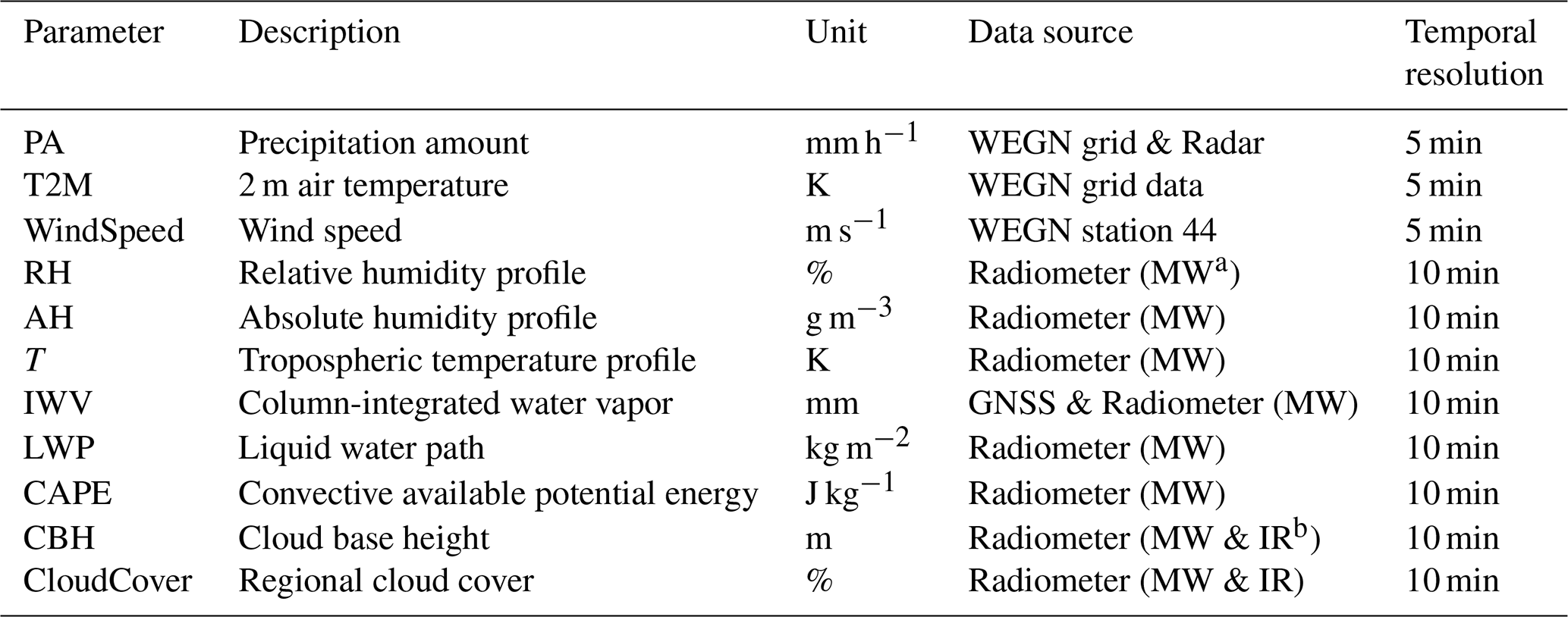
^a Microwave. ^b Infrared.

We further use all-sky scans of infrared brightness temperatures to detect cloud pixels (e.g., Feister et al., 2010) from which we compute the regional cloud cover (CloudCover). These observed quantities are aggregated to time series with 5 min (T2M, WindSpeed, PA) and 10 min (CBH, LWP, T, RH, AH, IWV, CloudCover) temporal resolution. Table 1 gives an overview of the parameters used in this study, together with their unit, data source and temporal resolution.

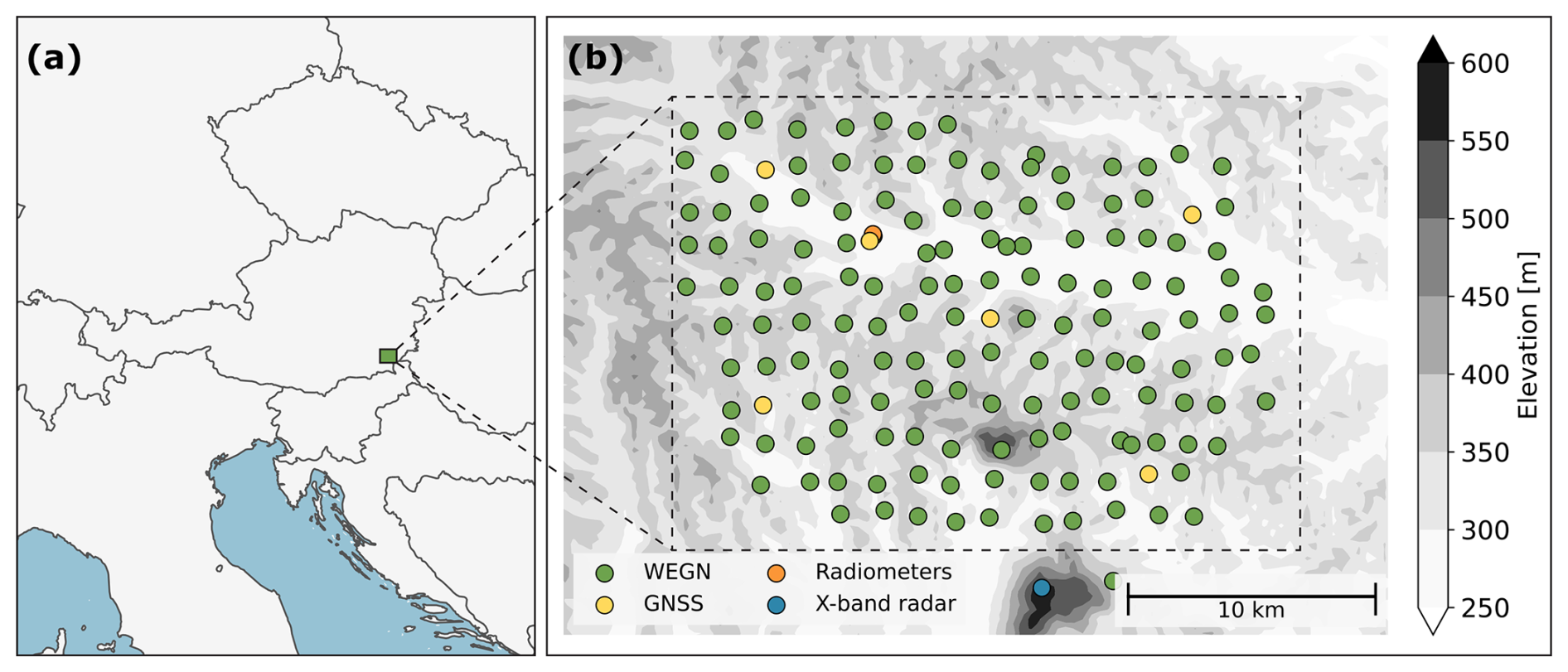
Figure 1 Location of the WEGN3D Open-Air Lab (a) and its individual stations (b). The colors of the circles indicate the station type: Green – climate station; orange – radiometer site (microwave/infrared and infrared); yellow – GNSS station; blue – X-band precipitation radar. The elevation (in m) is indicated by the gray colors.

The dataset covers the horizontal extent of the study area and has a vertical extent of approximately 250 to 10 km above mean sea level. T2M is given on a 100 m by 100 m terrain-following grid, which is obtained from the climate station observations by inverse distance weighted interpolation and local temperature lapse rates (Hocking, 2020). The radiometer site and the wind speed sensor, where CBH, CloudCover, LWP, T, RH, AH, and WindSpeed are observed, are located approximately at the center of the coverage area. For this study we decided to use the wind speed sensor that is located closest to the radiometer site to ensure that the measured wind speeds and the parameters obtained from the radiometers are connected to the same precipitation systems. The six-station GNSS network, that provides IWV, is evenly distributed throughout the coverage area. For spatially distributed data variables (PA, T2M, IWV), we compute the regional spatial mean and the regional spatial variability, represented by the standard deviation, to obtain a single representative time series. Figure 1 gives an overview of the sensor locations and coverage. We also compare the rainfall life cycle using reanalysis data, specifically ERA5 (Hersbach et al., 2023a, b), produced at the European Centre for Medium-Range Weather Forecasts in their 0.25° × 0.25° gridded version. This reanalysis provides the same data variables as the observational datasets used in this study, albeit with a coarser spatial and temporal resolution.

2.2 Methods

2.2.1 Case study event selection

Based on the WEGN event database, we select heavy precipitation events (HPEs) for our case study. The predominant type of precipitation in our study region is convective precipitation, which occurs mainly during the months of the warm season (April to October). We therefore first select all events from these months and discard the ones from the colder months (November to March). A detailed description of the WEGN event type classification is given in Appendix A. Furthermore, we only consider events that occurred later than 2020 to ensure that all of our observational data (climate station network, radiometers, GNSS, and radar) are available for all selected events. Given our focus on heavy precipitation, we require that our events have a maximum precipitation rate that exceeds the 90th percentile value (roughly 75 mm h⁻¹) of all recorded warm-season events. This results in a sample of 94 HPEs for our analysis. Note that due to the 5 min temporal resolution of the WEGN, hourly precipitation rates are derived by multiplying the 5 min precipitation amounts with a factor of 12.

2.2.2 Rainfall life cycle analysis

To analyze the life cycle of the HPEs recorded in the WEGN3D, we investigate 10 different parameters connected to heavy precipitation. The chosen parameters are: integrated water vapor (IWV), liquid water path (LWP), surface-based convective available potential energy (CAPE), 2 m air temperature (T2M) anomaly, air temperature profiles (T), cloud base height (CBH), cloud cover (CloudCover), wind speed (WindSpeed), relative humidity (RH), and absolute humidity (AH). Additionally, we inspect the temporal and spatial evolution of PA, T2M, and IWV during the events and have a quick look at the vertical profile of the temperature lapse rate (LR) before and after the event. Table 1 gives a detailed overview of the parameters. All parameters are directly available in the WEGN3D dataset except for the CAPE index, which we calculate from air pressure profiles, and radiometer-derived T and RH profiles using the MetPy Python package (May et al., 2022) Version 1.7.0 (https://unidata.github.io/MetPy/latest/index.html, last access: 12 May 2025), and the LR which we compute as the derivative of temperature along altitude. Note that due to the comparatively coarse resolution of the radiometer-derived temperature and humidity profiles, the resulting CAPE values are lower than, for example, radiosonde-derived ones (e.g., Gartzke et al., 2017). We thus focus on the temporal evolution of CAPE, rather than absolute values. The preprocessing steps are the same for all analyzed parameters. We select data from all time steps between 8 h before the event and the start of the event, as well as data from all time steps from the end of the event until 16 h after the event ends to investigate the event formation and dissipation.

For parameters which are provided on a spatial grid (T2M and CBH), we calculate the spatial mean value before the temporal selection to get a single time series for each parameter and event. To assess the precipitation life cycle in our observation data, we then calculate the median of all event samples per timestep for each of the above-mentioned parameters. Additionally, the 25th and 75th percentiles of all event samples per timestep are used as an indicator of the parameters' spreads around the event median. In some cases, anomaly time series reveal more about the development of HPEs than the time series of the absolute values. For these parameters (IWV, CBH, T2M, and AH), we first calculate the mean over the investigated time span (8 h before the event to 16 h after the event) and subtract it from the data before calculating the median and spread of the samples. Anomalies shown in this study should therefore be considered as “event anomalies”.

The data preparation and analysis procedures for ERA5 data are identical to those outlined above for the WEGN data. ERA5 provides all of the investigated parameters except absolute humidity, which we calculate from the pressure, temperature, and relative humidity data.

For the investigation of the precipitation stage (i.e., the part of the life cycle with rainfall), we focus on the maximum precipitation amount, the 2 m air temperature anomaly, and the IWV anomaly, as well as their spatial variability. We normalize the duration of each single event to make them comparable and repeat the data preparation steps described above.

3 Results

First, we investigate some general event statistics of the 94 HPEs selected by the methods described in Sect. 2.2.1 (Fig. 2). HPEs are by nature quite intense and short events, i.e. all of the precipitation accumulates in a short period of time. This is reflected in high maximum precipitation rates of more than 50 mm h⁻¹ (Fig. 2a), comparatively low mean precipitation rates below 5 mm h⁻¹ (Fig. 2b), and event durations shorter than 4 h (Fig. 2c). We find more HPEs during the afternoon (Fig. 2d) and during the warmer summer months June–August (Fig. 2e). This is due to the close link of convective precipitation to temperature. As mentioned above, the predominant precipitation type in our study region during the warm season is convective. This is also clearly visible in the histograms of the event statistics, where most events are classified as convective or mixed events (Fig. 2f), meaning that they have at least a convective part.

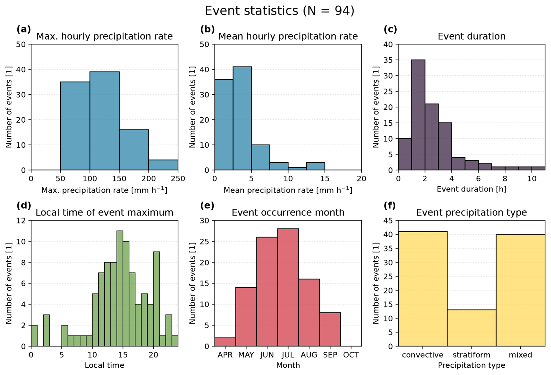
Figure 2 Event statistics of the 94 HPEs selected for the study. (a) Maximum hourly precipitation rate in mm h⁻¹, (b) mean hourly precipitation rate in mm h⁻¹, (c) event duration in hours, (d) local time of event maximum, (e) month of event occurrence, and (f) precipitation type classified by the WEGN event classification (see Appendix A).

3.1 Event formation and dissipation stages

Next, we are interested in the development of multiple parameters that are linked to HPEs from 8 h before to 16 h after the event (Fig. 3). First, we focus on the WEGN3D data (solid colored lines in Fig. 3). Like Wang and Hocke (2022), we find that the median IWV anomaly increases in the hours prior to the event. During the event, the IWV anomaly drops by about 2 mm, followed by a continuous gradual decline during the hours after the event. The LWP is mostly constant throughout the investigated time span with a sharp increase of roughly 0.4 kg m⁻² in the hour directly before the event onset and a clear drop after the event. Both, the IWV anomaly and the LWP, represent the increase of water (liquid and gaseous) in the atmosphere before HPEs. After the events, the water precipitated to the surface, and both the IWV anomaly and the LWP have lower levels than before. The magnitude of these increases and drops is also well above the IWV and LWP measurement uncertainty, given the sample size of 94 events. Further, we find a clear build up of CAPE, peaking 1 h before the event onset, followed by a drastic drop of nearly 300 J kg⁻¹, underlining the convective character of the investigated events. The time lag between the CAPE peak and the event onset is the result of deep convection, which weakens CAPE through multiple mechanisms. One of these mechanisms is the warming of the upper air layers as a result of the upward transfer of latent heat released during condensation, resulting in a more stable atmosphere. This stabilizing effect is further supported by the cooling of the lower atmosphere through downdrafts (Barbero et al., 2019). There are multiple mechanisms that can explain the decrease in CBH anomaly of about 1000 m detected close to the event onset. Connected to the increase in IWV anomaly described above, a lowering of the lifting condensation level could result in a lowering of the CBH. However, we also find that most HPEs observed do not form within the comparatively small region of the WEGN. This means that before a HPE the sky is either clear or filled with some fair-weather clouds which get displaced by cumulus clouds close to the actual event, which could also lead to the observed decrease in CBH. Concerning temperature, we find that the 2 m air temperature anomaly is roughly 5.5 K lower after the event than it was directly before the beginning of the event. The wind speed anomaly exhibits a stark rise (+1.5 m s⁻¹) before the event and is mainly constant in the hours following the end of the event.

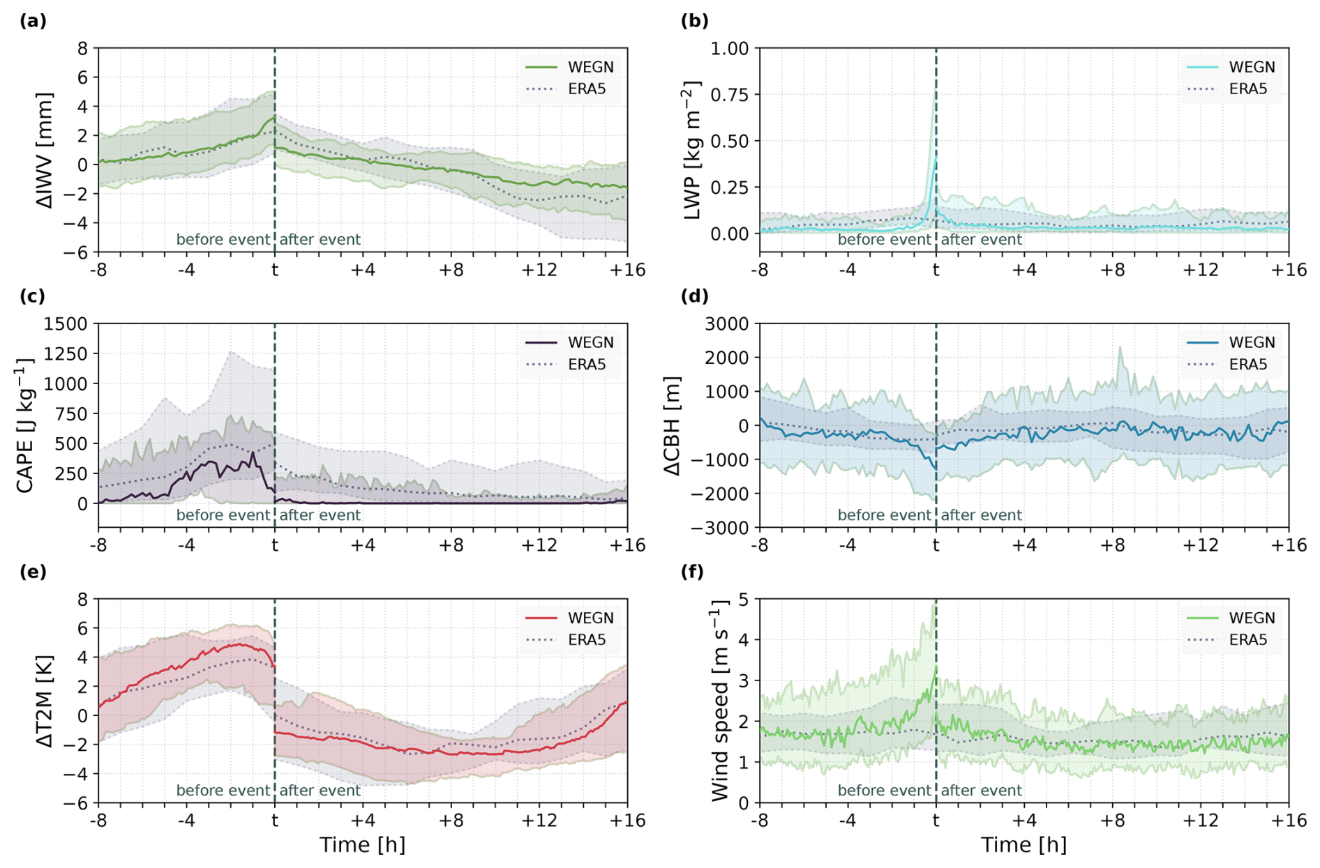
Figure 3 Climatology of different HPE parameter from 8 h before to 16 h after the event for WEGN3D data (solid colored lines) and ERA5 (dotted gray lines). The time is given as t ± hours after/before the event. The dashed line marks the event t, since the hours of the event itself (i.e., when rainfall occurred) are not depicted here. The parameters shown are: IWV anomaly (a), LWP (b), CAPE (c), CBH anomaly (d), 2 m air temperature anomaly (e), and wind speed anomaly (f). The lower and upper edges of the shaded corridors correspond to the 25th and 75th percentiles respectively.

Figure 3 additionally shows the precipitation life cycle in the ERA5 data (dotted gray lines). ERA5 describes the general tendencies of IWV anomaly, CAPE, and T2M anomaly before and after the event well, despite the lower spatial and temporal resolution of the dataset. This is in line with the expected physical behavior. Cloud and wind related parameters do, however, not show any patterns related to the HPEs.

Figure 4 Median vertical structures of temperature anomaly (a, d), relative humidity (b, e), and absolute humidity anomaly (c, f) for WEGN3D (a–c) and ERA5 (d–f) from 8 h before to 16 h after the event. The time is given as t ± hours before/after the event. The dashed line marks the event t. The temperature anomalies are shown for the lower atmosphere up to 2 km, the other parameters up to 10 km.

Using the atmospheric sounding capabilities of the WEGN3D Open-Air Lab, we now investigate the vertical structure of temperature anomaly, relative humidity, and absolute humidity anomaly before and after the event (Fig. 4a–c). In agreement with the 2 m air temperature anomalies shown above, we find a stark contrast in air temperature of up to 6.5 K between the time before and after the event. Considering that our events mainly occur in summer in the afternoon (Fig. 2), high temperature anomalies are linked to high absolute temperatures, which are one of the key ingredients of convective precipitation. The high temperature anomalies found in Fig. 4a therefore further underline the convective nature of our events. As an indicator for the atmosphere's stability, we additionally investigate the environmental lapse rate (LR), shown in Appendix B, Fig. B1. Before the event onset, we observe high LR values that point towards an unstable, and hence a thunderstorm favoring, atmosphere (Daidzic, 2019). In the hours after the event, we observe decreased LR values and a persistent inversion layer at roughly 500 m. Figure 4a shows that the temperature difference between pre and after event is higher at lower altitudes, which we attribute to the increased moisture at these levels. As a consequence, the lower layers are cooler after the event then higher layers, resulting in an inversion layer. At higher altitudes the decrease in LR values might be connected to the release of latent heat during the rainfall event. Further, due to the events' tendency to occur mainly in the afternoon, the hours after the event are often during the night time, where radiation effects often lead to LR inversions.

Another characteristic of convective precipitation can be observed in Fig. 4b where the vertical structure of relative humidity is shown. Areas with high relative humidity values enable us to make assumptions about the location and extent of the cloud. These areas form and expand vertically close to the event onset, corresponding to the arrival of the convective cloud system. Using the lower contour of the 80 %–90 % RH area as a proxy for the CBH, we see a decrease in CBH of about 2 km in the 2 h before the event. This roughly corresponds to the drop in CBH anomaly already detected in Fig. 3d. To complement the findings of the vertical structure of temperature anomaly and relative humidity, we also investigate the absolute humidity anomaly (Fig. 4c). As one might expect, the absolute humidity anomalies are higher (by roughly 2 g m⁻³) in the time before the event than they are in the time after the HPEs occurred. The smaller values of absolute humidity anomalies in the time after the event can be explained by air moisture precipitating to the ground, and also from the fact that the air is colder after the event occurred and can hence hold less moisture than before.

Again, we are also studying the life cycle using the reanalysis dataset. For that purpose, we examine the vertical structure of temperature anomaly, relative humidity, and absolute humidity anomaly in ERA5 data (Fig. 4d–f). The general pattern in temperature anomaly of higher values before the event and lower ones after is also visible in the ERA5 data. We find temperature anomalies in the range of ±2 K with a shift from high to low anomalies about 3 h after the event. The sharp drop in temperature during the last hour before the event is, however, less pronounced in ERA5 compared to the WEGN3D data. We attribute this to the coarser time resolution of the reanalysis, which may not be able to accurately capture sudden changes in the pre-rainfall environment. Concerning relative humidity, the HPEs seem to have an effect on ERA5 RH values at higher altitudes of about 5–8 km, where RH increases for a short period after the event before returning to its pre-event levels. The RH can be used to get an idea of the rough locations of the storm cloud. In agreement with the CBH anomalies shown in Fig. 3, the clouds are relatively stable over the whole observed time span, showing no indication of the arrival of the convective cloud system. Similar to the patterns found in the temperature anomalies, the absolute humidity anomalies also exhibit positive values up to about 4 h after the event, and negative values afterwards. The elevated AH anomalies are all located below 3 km and have values in the range of ±1 g m⁻³. The comparatively coarse vertical resolution of the radiometer-derived WEGN temperature and humidity profiles is evident, with very little vertical variation visible above 1.5–2 km.

Figure 5a shows that the median regional cloud cover exhibits a large spread in the time span between 8 and 2 h before the event, but starts to consistently increase towards 100 % at 2 h before the event onset. This increase in cloud cover coincides with the T2M maximum, which also occurs approximately 2 h before the event (see Fig. 3e). Following the T2M maximum, the surface cooling effect of the increased cloud cover, reduced cloud base height, and increased LWP (see Fig. 3d and b) is then clearly visible in the T2M time series (see Fig. 3e). The spatial variability in T2M (Fig. 5b) starts to increase consistently by 0.2 K in the last hour before the event. While this is considerably later than the cloud cover increase, it coincides with the sudden increase in LWP (see Fig. 3b) before the event. This suggests that a thicker cloud layer is required for localized cooling to occur. Another reason for the increase in temperature variability might come from convective cold pools (Kirsch et al., 2024) which are often detected at the location of HPEs before the event onsets. While we do find indications of such cold pools for a few of the investigated HPEs (not shown), most of the HPEs do not form directly in the region covered by the WEGN, which means that potential cold pools cannot be found in that area as well. After the event, we see a substantial drop in T2M variability which indicates that rainfall and persistent cloud cover lead to a homogeneous horizontal temperature distribution.

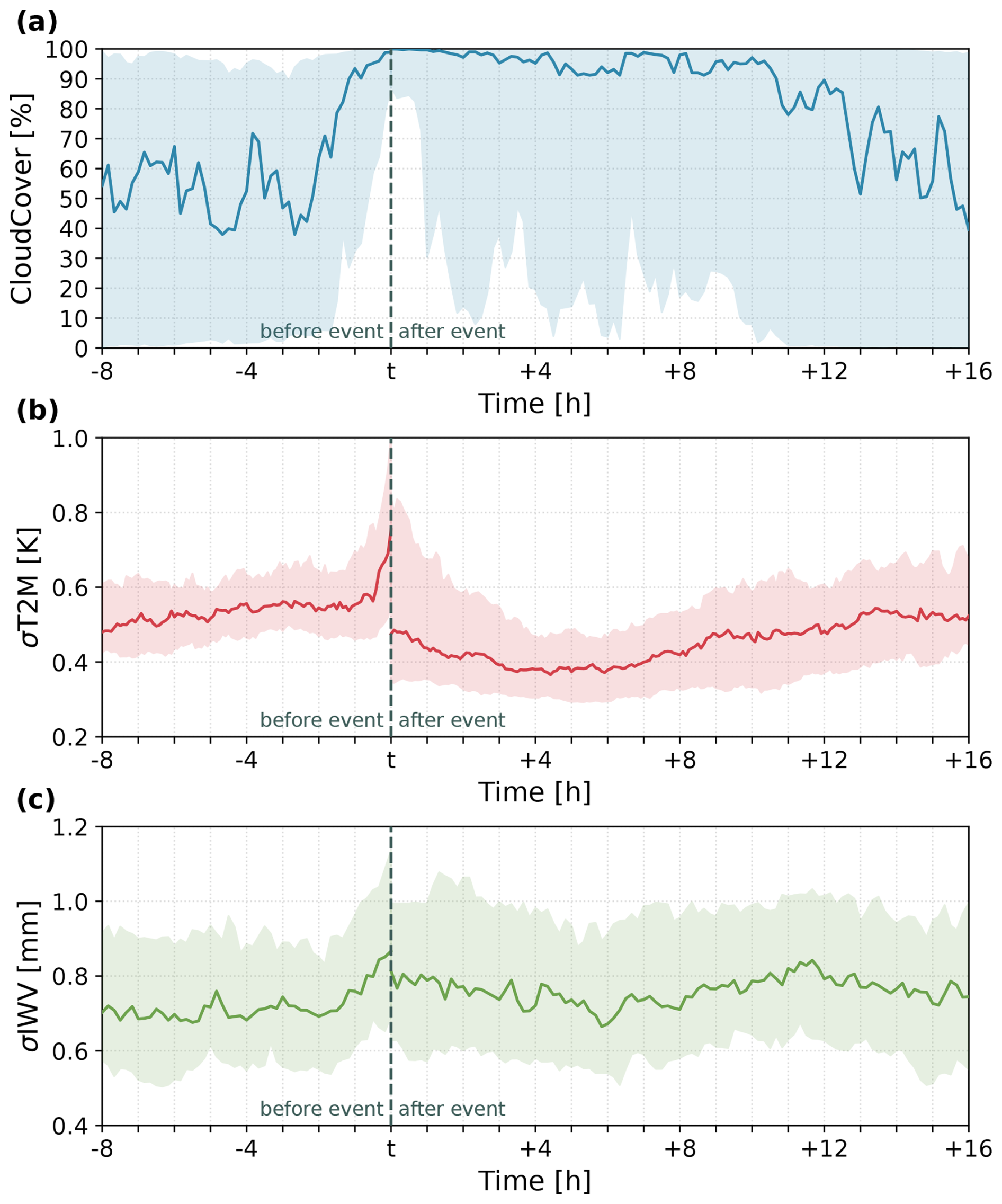
Figure 5 (a) Temporal evolution of regional cloud cover (CloudCover) for all events, from 8 h before to 16 h after the event. Median spatial variability of (b) 2 m air temperature (σT2M) anomaly and (c) integrated water vapor anomaly (σIWV) for all events, from 8 h before to 16 h after the event. The time is given as t ± hours before/after the event. The dashed line marks the event t. The lower and upper edges of the shaded corridors correspond to the 25th and 75th percentiles respectively.

Figure 5c shows an increase in IWV spatial variability that already starts approximately 2 h before the precipitation stage. This indicates the onset of convection (Weckwerth, 2000). After the event, the IWV variability drops to pre-event levels.

3.2 Precipitation stage

The precipitation stage of each event starts with the first recorded occurrence of surface rainfall in the study area and lasts until precipitation ceases. In this event stage, we focus our analysis on the spatial and temporal variability of PA, T2M, and IWV, and their interaction. Profiles of RH, AH, and T, as well as time series CBH and LWP are not available during the precipitation stage, as the microwave radiometer observations used in their retrieval become heavily biased once the instrument is coated with water (Löhnert and Crewell, 2003). To avoid these biases influencing our analysis, we exclude all microwave radiometer observations between the first recorded rainfall and 30 min after the last recorded rainfall at the radiometer site. Since the duration of the vast majority of events is similar, around 2 h (see Fig. 2), we normalize their duration to make them comparable. Figure 6 shows a snapshot of the regional T2M anomaly, along with accumulated precipitation amounts (from event start to 20 min into the event) derived from radar and gauge measurements, 20 min into the event on 15 September 2022. The T2M anomaly is calculated by subtracting the spatial mean over the whole region from the data. We can see that the spatial pattern of the near-surface cooling is highly correlated with the accumulated precipitation amount, as a direct consequence of the cooler precipitation hitting the ground and subsequent evaporation.

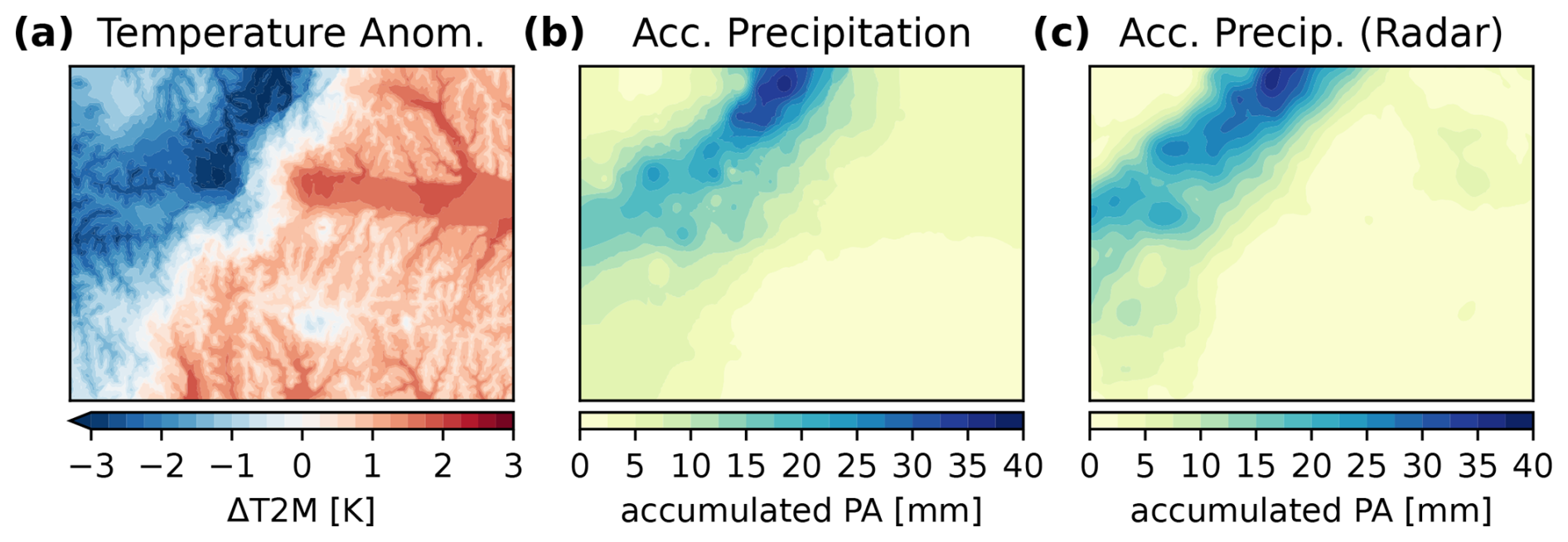
Figure 6 Snapshot of the 2 m near surface temperature (T2M) regional anomaly in panel (a) and accumulated precipitation amount from radar and rain gauges in panels (b) and (c), 20 min into the event on 15 September 2022.

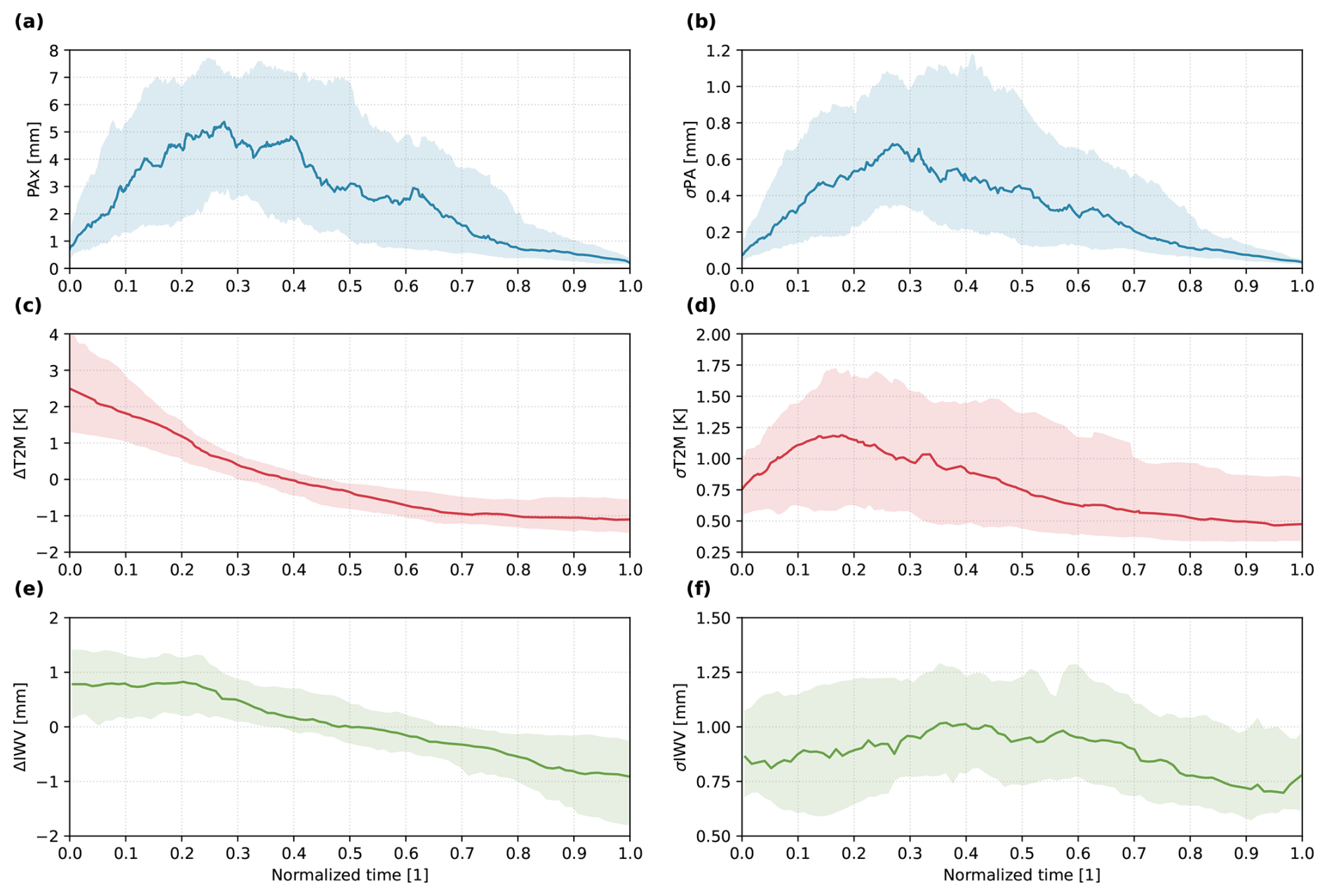
Figure 7 Median (a) maximum precipitation amount, (b) spatial variability of precipitation amount, (c) 2 m air temperature anomaly, (d) spatial variability of T2M, (e) median IWV anomaly, and (f) spatial variability of IWV for all events during the precipitation stage. The lower and upper edges of the shaded corridors correspond to the 25th and 75th percentiles respectively.

Figure 7 depicts the development of the maximum 5 min precipitation amount (PAx), 2 m air temperature anomaly, and IWV anomaly during the event, as well as, the spatial variability of these parameters. The temperature anomaly is again calculated with the steps described in Sect. 2.2.2. The steady increase in PAx up until about 27 % into the event corresponds with the rain cell entering the FBR region. A large amount of the investigated HPEs are of mixed precipitation type (Fig. 2f), meaning that the events could consist of a convective event that is directly followed by a stratiform event which is probably the reason for the slower decrease in PAx after the peak. This results in the asymmetric behavior of PAx found in Fig. 7a. Another effect of these stratiform follow-up events is the small spread of PAx towards the end of the events. The spatial variability of precipitation during the event (Fig. 7b) matches the development of PAx described above. Again, the spread here illustrates the highly localized character of the events, as well as the effect that some of the events are displaced by stratiform events towards the end.

As already shown and described above, near-surface cooling is highly correlated with the accumulated precipitation amount (Fig. 7c, d). The T2M anomaly steadily decreases throughout the whole event, resulting in roughly 3 K colder temperatures at the end of the event in comparison to the event onset. For the spatial variability of T2M, the maximum occurs at approximately 15 % into the event which amounts to 18 min for a 2 h rainfall event. At this stage, the study region is only partially affected by precipitation, leading to localized precipitation-induced cooling. Once precipitation occurs in the whole study region, the temperature reduction becomes more uniform, resulting in a reduction of T2M spatial variability. The strong correlation between the spatial patterns of PA and T2M is also evident in the almost identical temporal evolution of the PA spatial variability (Fig. 7b), indicating that the precipitation-induced cooling is also the main driver behind the temporal evolution of the T2M spatial variability shown in Fig. 7f.

Finally, we have a look at the IWV anomaly during the event (Fig. 7e). Similar to the T2M anomaly, the IWV anomaly exhibits a decrease during the time of rainfall. The spatial variability of IWV shown in Fig. 7f also follows a pattern similar to that of T2M, with an increase in variability until 30 % of the event duration, followed by a slow decrease. The maximum of the median spatial IWV variability with 1 mm is substantially higher during the precipitation stage than before and after the event, where we observe a range of 0.7–0.8 mm. This is a consequence of local cooling in rainfall-affected areas and the subsequent reduced capacity of the air column to hold water vapor, as well as the sensitivity of GNSS- and radiometer-derived IWV to liquid water in the atmosphere (Solheim et al., 1999; Löhnert and Crewell, 2003). The amount of IWV slowly decreases by about 13 % over the course of the precipitation phase. This contrasts the findings of Wang and Hocke (2022), who only find a minor reduction in IWV for precipitation events shorter than 8 h. We attribute this different behavior to the fact that the events in our study only take place in the warm season and are primarily of convective nature, which results in higher air temperatures before the events. Combined with the lower altitude of the study region, the absolute IWV we observe is higher, and thus also the potential for a larger IWV reduction is higher.

4 Discussion

The life cycle analysis of 94 heavy precipitation events confirmed that these events are mainly of convective nature in our study region, which is characterized by its close link to temperature, short durations, and high intensities. Before we discuss the investigated life cycle of HPEs in observation and reanalysis data, it is important to remember how such HPEs usually unfold: let's assume a typical summer day with morning temperatures that are already well above 20 °C. During the day, the temperature further rises and the first clouds begin to form. The sky darkens and is slowly filled with towering cloud formations, while a gentle breeze transforms into strong winds. Shortly afterwards, the first raindrops begin to fall. Within minutes, the rainfall intensifies drastically and we are in the middle of a full-grown heavy convective precipitation event.

Considering this typical life cycle of HPEs in our study region, we find that the physical processes and effects connected to these events are adequately represented in the WEGN3D data. We clearly detect local precursors of HPEs, such as the rise in temperature, illustrated by the temperature anomaly shown in Figs. 3e and 4a. The energy build-up, which co-occurs with a rise in temperature, is reflected by the increase of CAPE in the hours prior to the event onset (Fig. 3c). The drop of the cloud base height anomaly prior to the event (Figs. 3d and 4b) corresponds to the expected arrival of the convective cloud system and the strong rise in wind speed before the event onset is also clearly visible in the WEGN3D data (Fig. 3f). During the precipitation stage, precipitation triggers a cooling effect, which we consider to be the main driver of the temporal evolution of the T2M spatial variability during the time of rainfall. This proves the WEGN3D's capability to capture the characteristics of high-intensity small-scale rainfall events with unique detail.

Our findings are not only physically plausible, they are also in agreement with previous studies. The observed increase in IWV anomaly before event onset confirms the findings of previous studies such as Benevides et al. (2015), Sapucci et al. (2019), Wang and Hocke (2022), and Wang et al. (2024). Since all of these studies focus on different regions (Benevides et al., 2015: Portugal; Sapucci et al., 2019: Brazil; Wang and Hocke, 2022: Swiss Plateau; Wang et al., 2024: Andalusia, Spain; this study: Austria), the observed rise in IWV (anomaly) seems to be a fundamental feature of heavy (convective) precipitation events. Furthermore, the rapid increase in LWP before HPEs, and the increased levels of RH after a rainfall event, are in agreement with the findings of Wang and Hocke (2022), which gives indications for further characteristic features of HPEs in observation data.

The WEGN3D's capability to adequately capture very characteristic features of high-intensity small-scale rainfall events while being solely observation-based (i.e., generated without any models) illustrates the high potential for applications of this dataset in the improvement and verification of weather and climate models. Specifically, the data could be used to develop an experimental nowcasting model for the region. Of particular interest could be the added value of using atmospheric precursors of (heavy) precipitation in addition to extrapolation-based nowcasting methods (cf. Bojinski et al., 2023; Wang et al., 2024). Given the holistic setup of the instruments, such a model can be adjusted and verified in a very fine-grained manner, potentially serving as a blueprint for improving larger-scale models. Another potential application is the verification of high-resolution weather models by comparing the temporal evolution of the parameters examined in this study (cf. Table 1) with the corresponding model outputs. The models could also be tuned to more accurately reproduce the observed behavior of these parameters.

As mentioned in the Introduction, our study region is highly affected by convective rainfall events, which are particularly hazardous and often result in serious damage and socioeconomic losses (Schroeer and Tye, 2019). Although the FBR is comparatively small (22 km × 16 km), it can still be used as a representative example for the larger surrounding region in terms of (seasonal) precipitation amount and predisposition to convective precipitation (Lombardo and Bitting, 2024), making the findings of this study also applicable for a larger geographical region. Considering the projected increase of these events in a warming climate (IPCC, 2021), the threat posed by heavy precipitation events will likely increase over time as well. Understanding HPEs in great detail and being able to monitor them correctly is therefore a crucial skill, which is especially important for highly affected regions such as the southeastern Alpine forelands and its surroundings. Our study shows that the WEGN3D dataset can play an important role in this difficult and important task.

5 Conclusions

This study investigates the life cycle of 94 heavy precipitation events in observation (WEGN3D) and reanalysis (ERA5) data in the southeastern Alpine forelands, to answer the following research questions:

• How do specific atmospheric parameters evolve in the hours before and after heavy precipitation events?

• What spatial effects does rainfall have on surface parameters and moisture distribution?

With respect to the first research question, we find that in the hours prior to an HPE the IWV anomaly, LWP, CAPE, 2 m air temperature anomaly, and wind speed increase, while the CBH anomaly decreases. In the hours following an HPE all of these parameters drop drastically, except for the CBH anomaly which rises back up to pre-event levels. These findings are well in line with previous studies and the expected physical behavior of such events.

In the hour before the event onset, the spatial T2M variability starts to increase, coinciding with the increase detected in LWP (i.e., the thickening of the cloud system). In addition, the spatial IWV anomaly variability indicates the onset of convection in the 2 h prior to the event. The rainfall itself leads to a localized cooling effect, which is clearly visible in the spatial variability of T2M and IWV anomaly during the event. After the event, a homogeneous horizontal temperature distribution is detectable.

Our study shows that despite being solely based on observations, the WEGN3D is very skilled in monitoring HPEs and their characteristics, which illustrates the dataset's high potential for the utterly relevant application in the improvement and verification of weather and climate models.

Appendix A: Precipitation event classification

To classify HPEs, we make use of 5 min gridded T2M and gridded PA to characterize periods of precipitation within the 22 km × 16 km study region, in terms of their duration, precipitation amount, precipitation intensity, spatial variability, precipitation-affected area, precipitation phase, and convective potential. A precipitation event is defined as a contiguous sequence of epochs where the maximum 5 min precipitation amount exceeds 0.19 mm (at least two bucket tips in 5 min), the average 5 min precipitation amount exceeds 0.0039 mm (at least 0.05 mm h⁻¹), or where the maximum 5 min precipitation amount exceeds 0.009 mm (at least one bucket tip in 5 min) if the 5 min gridded T2M is below 2 °C. If a time period is identified as a precipitation event, we compute further statistics from the K epochs contained in the event. The statistics include the regional T2M average T_A over all M grid points for the event duration, defined as

$$\begin{array}{}\text{(A1)}& T_{\mathrm{A}}={\displaystyle \frac{\mathrm{1}}{M}}\sum _{i=\mathrm{0}}^{M-\mathrm{1}}{\displaystyle \frac{\mathrm{1}}{K}}\sum _{k=\mathrm{0}}^{K-\mathrm{1}}T(t_k,{\mathit{x}}_i),\end{array}$$

where T(t_k,x_i) is the 5 min T2M at the grid point i and epoch k. Additionally, the fractional area at which precipitation occurred, F_PA, is defined as

$$\begin{array}{}\text{(A2)}& F_{\mathrm{PA}}={\displaystyle \frac{\mathrm{1}}{A}}\sum _{i\in S}{a}_i\end{array}$$

with

$$S=\left\{i\left|\left(\sum _{k=\mathrm{0}}^{K-\mathrm{1}}\mathrm{PA}(t_k,{\mathit{x}}_i)\right)\right.>\mathrm{0.09}\mathrm{mm}\right\},$$

where a_i is the area associated with the ith grid point and A is the total area covered by the grid data product. We further compute the maximum fractional area covered by precipitation F_PM on at least one epoch with

$$\begin{array}{}\text{(A3)}& F_{\mathrm{PM}}=max\left\{\left.{\displaystyle \frac{A_k}{A}}\right|k\in \mathit{\{}\mathrm{0},\mathrm{\dots },K-\mathrm{1}\mathit{\}}\right\}\end{array}$$

with

$$A_k=\sum _{i\in S_k}{a}_i$$

and

$$S_k=\mathit{\left\{}i\right|\mathrm{PA}(t_k,{\mathit{x}}_i)>\mathrm{0.09}\mathrm{mm}\mathit{\}},$$

and the normalized spatial variability N_SV defined as

$$\begin{array}{}\text{(A4)}& N_{\mathrm{SV}}={\displaystyle \frac{\mathrm{1}}{{\stackrel{\mathrm{‾}}{\stackrel{\mathrm{‾}}{P}}}_{\mathrm{R}}}}{\displaystyle \frac{\mathrm{1}}{M-\mathrm{1}}}\sum _{i=\mathrm{0}}^{M-\mathrm{1}}{\left({\stackrel{\mathrm{‾}}{P}}_{\mathrm{R}}\left({\mathit{x}}_i\right)-{\stackrel{\mathrm{‾}}{\stackrel{\mathrm{‾}}{P}}}_{\mathrm{R}}\right)}^{\mathrm{2}},\end{array}$$

where

$${\stackrel{\mathrm{‾}}{P}}_{\mathrm{R}}\left({\mathit{x}}_i\right)={\displaystyle \frac{\mathrm{1}}{K}}\sum _{k=\mathrm{0}}^{K-\mathrm{1}}\mathrm{PA}(t_k,{\mathit{x}}_i),$$

and

$${\stackrel{\mathrm{‾}}{\stackrel{\mathrm{‾}}{P}}}_{\mathrm{R}}={\displaystyle \frac{\mathrm{1}}{M}}\sum _{i=\mathrm{0}}^{M-\mathrm{1}}{\displaystyle \frac{\mathrm{1}}{K}}\sum _{k=\mathrm{0}}^{K-\mathrm{1}}\mathrm{PA}(t_k,{\mathit{x}}_i).$$

The maximum precipitation sum P_SM is defined as

$$\begin{array}{}\text{(A5)}& {\displaystyle }{P}_{\mathrm{SM}}=max\left\{\left.\sum _{k=\mathrm{0}}^{K-\mathrm{1}}\mathrm{PA}(t_k,{\mathit{x}}_i)\right|i\in \mathit{\{}\mathrm{0},\mathrm{\dots },M-\mathrm{1}\mathit{\}}\right\}.\end{array}$$

Together with the event duration D, these features allow us to further divide precipitation events into the classes convective, stratiform, mixed, weak, and snow. Convective-class events are characterized by high precipitation intensity, high spatial variability, small spatial extent, and a high-enough surface temperature to allow for convection. Stratiform-class events exhibit low spatial variability, large spatial extent, longer duration, and lower surface temperatures. An event is classified as mixed when it cannot be unambiguously identified as convective or stratiform. This typically occurs when convective precipitation is followed by prolonged rainfall with decreasing intensity. The remaining two classes, which are not considered in this study, are snow which can only occur when the surface temperature is close to the freezing level and weak with a very low mean precipitation amount.

These class definitions are realized in a decision tree structure, which is applied to the grid-derived features in daily chunks from 06:00 to 06:00 UTC. The numerical values of the splitting rules are derived empirically and can be found in Fig. A1. An overview of the parameters used for the event classification is given in Table A1.

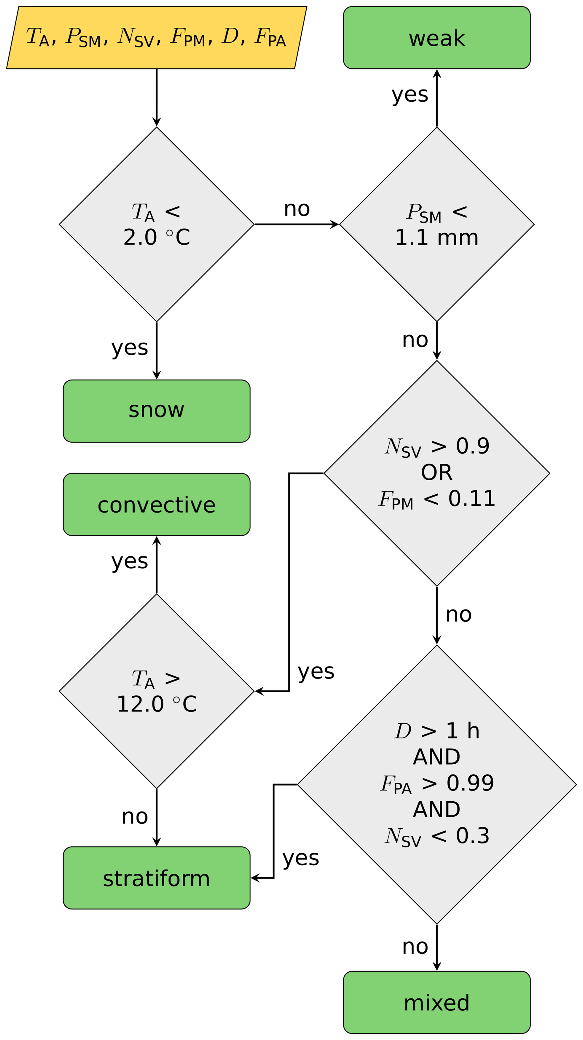
Figure A1 Event classification decision tree based on the features regional T2M average (T_A), maximum precipitation sum (P_SM), normalized spatial variability (N_SV), maximum fractional area covered by precipitation (F_PM), event duration (D), and fractional area at which precipitation occurred (F_PA).

Table A1 Parameters used for the event classification algorithm.

Appendix B: Lapse rate analysis

As an additional parameter, we have a look at the vertical structure of the environmental lapse rate (LR), which is shown in Fig. B1. The LR is calculated from WEGN3D temperature data as the derivation by height.

Figure B1 Median vertical structures of the environmental lapse rate (LR) for WEGN3D from 8 h before to 16 h after the event. The time is given as t ± hours before/after the event. The dashed line marks the event t.