the Creative Commons Attribution 4.0 License.
the Creative Commons Attribution 4.0 License.
 | 28 Oct 2020
Attribution of precipitation to cyclones and fronts over Europe in a kilometer-scale regional climate simulation
Stefan Rüdisühli
Michael Sprenger
David Leutwyler
Christoph Schär
Heini Wernli
This study presents a detailed analysis of the climatological distribution of precipitation in relation to cyclones and fronts over Europe for the 9-year period 2000–2008. The analysis uses hourly output of a COSMO (Consortium for Small-scale Modeling) model simulation with 2.2 km grid spacing and resolved deep convection. Cyclones and fronts are identified as two-dimensional features in 850 hPa geopotential, equivalent potential temperature, and wind fields and subsequently tracked over time based on feature overlap and size. Thermal heat lows and local thermal fronts are removed based on track properties. This dataset then serves to define seven mutually exclusive precipitation components: cyclonic (near cyclone center), cold-frontal, warm-frontal, collocated (e.g., occlusion area), far-frontal, high-pressure (e.g., summer convection), and residual. The approach is illustrated with two case studies with contrasting precipitation characteristics. The climatological analysis for the 9-year period shows that frontal precipitation peaks in winter and fall over the eastern North Atlantic and the Alps (> 70 % in winter), where cold frontal precipitation is also crucial year-round; cyclonic precipitation is largest over the North Atlantic (especially in summer with > 40 %) and in the northern Mediterranean (widespread > 40 %); high-pressure precipitation occurs almost exclusively over land and primarily in summer (widespread 30 %–60 %, locally >80 %); and the residual contributions uniformly amount to about 20 % in all seasons. Considering heavy precipitation events (defined based on the local 99.9th all-hour percentile) reveals that high-pressure precipitation dominates in summer over the continent (50 %–70 %, locally >80 %); cold fronts produce much more heavy precipitation than warm fronts; and cyclones contribute substantially (50 %–70 %), especially in the Mediterranean in fall through spring and in northern Europe in summer.
- Article
(35132 KB) - Full-text XML
-
Supplement
(20792 KB) - BibTeX
- EndNote


Precipitation is one of the most central meteorological variables. Therefore, huge efforts have been invested in compiling regional and global precipitation climatologies from surface station measurements, remote-sensing data, and combinations thereof (e.g., Xie and Arkin, 1997; Frei and Schär, 1998; Adler et al., 2003; Sun et al., 2018; Isotta et al., 2014). Such climatologies with typically monthly time resolution serve to characterize the spatial patterns, seasonal cycle, and interannual variability of precipitation, and they are valuable for strategic decisions in different socioeconomic sectors (e.g., water management, agriculture, hydropower generation). Long-term climatologies reveal large interannual variability and trends (e.g., Klein Tank and Können, 2003; Zolina et al., 2010). Among the most important questions for future climate change is how a warmer climate will affect precipitation and its climatological distribution, seasonality, interannual variability, and the occurrence of extreme events. In the global mean, precipitation is expected to increase at a rate of 2 % per degree of global-mean warming, but changes in short-term precipitation are likely to occur at much faster rates (Trenberth, 1999; Held and Soden, 2006; Schneider et al., 2010). In the last decade, huge progress has been made in realistically simulating the hydrological cycle with high-resolution climate models, including the spatial distribution of precipitation, its diurnal cycle, and the statistics of extreme events (e.g., Hohenegger et al., 2008; Kendon et al., 2012; Ban et al., 2014, 2015; Prein et al., 2015; Clark et al., 2016; Keller et al., 2016; Leutwyler et al., 2017). A major part of this progress is due to the step change of simulating deep convection explicitly instead of using a parameterized representation. In their systematic comparison of climate model simulations with parameterized or explicit convection, Prein et al. (2015) found that “Improvements [when using explicit convection] are evident mostly for climate statistics related to deep convection, mountainous regions, or extreme events.”
An important aspect of understanding the precipitation climatology and, eventually, its sensitivity to climate change is the linkage of precipitation to synoptic-scale weather systems. As outlined below, extratropical cyclones, fronts, orography, high-pressure systems, and their interactions contribute essentially to the formation of precipitation in the midlatitudes, including extreme events related to deep convection. Research in this area has so far mainly followed two strands: (i) detailed investigations of specific high-impact precipitation events, their large-scale precursors, and mesoscale dynamics (e.g., Buzzi et al., 1998; Massacand et al., 1998; Zängl, 2007; Stucki et al., 2012; Grams et al., 2014; Piaget et al., 2015) and (ii) global climatologies to quantify the relevance of cyclones, fronts, warm conveyor belts, and atmospheric rivers for total and/or extreme precipitation (e.g., Catto et al., 2012; Pfahl and Wernli, 2012; Catto and Pfahl, 2013; Lavers and Villarini, 2013; Pfahl et al., 2014; Hénin et al., 2019). However, most climatological studies on the relationship between precipitation and synoptic weather systems are based on global reanalyses with a typical resolution of 100 km in space and 6 h in time. Such resolution is clearly inadequate to capture phenomena like short-duration convective precipitation events or the complex interplay between fronts and steep topography in producing precipitation. In addition, a distinction between convective and stratiform precipitation is challenging at such resolutions. While some models distinguish stratiform (explicit) and convective (parameterized) precipitation, the convective fraction strongly depends on the model (see Fig. 3 in Fischer et al., 2015).
This study aims to fill these gaps by using high-resolution data to quantify the co-occurrence of precipitation and a set of weather systems over Europe in the present-day climate. A kilometer-scale climate simulation with explicit convection provides the ideal database to perform such a methodologically and computationally demanding analysis.
Explaining the surface precipitation pattern has been a major aspect of the Norwegian cyclone model, introduced almost a century ago by Bjerknes and Solberg (1922). They realized that most cyclones are associated with a warm front, which slopes gently forward with height and produces widespread, rather uniform precipitation of moderate intensity, followed by a cold front, which is steeper, slopes rearward with height, and produces much more intense but less widespread precipitation (Bjerknes, 1919). In the time since, several aspects of the original Norwegian model have been revised, and new features of extratropical cyclones have been introduced. On the large scale, an important addition has been the concept of characteristic airstreams, among them the warm conveyor belt, a warm and moist airstream that ascends along and ahead of the cold front and overruns the warm front, all the while producing large amounts of precipitation (Harrold, 1973; Pfahl et al., 2014). Recent studies suggest that embedded convection can occur within the mostly stratiform cloud band formed by this airstream, leading to intense peaks in surface precipitation (Neiman et al., 1993; Flaounas et al., 2016; Oertel et al., 2019). Observational studies have also revealed complex mesoscale structures in and around the large-scale frontal precipitation areas. In the vicinity of the warm front, there may be about 50 km wide, intense warm-frontal rainbands (e.g., Herzegh and Hobbs, 1980; Colle et al., 2017). In the comparatively dry warm sector, isolated mesoscale precipitation areas about 10 to 100 km in size can occur, which are triggered by large-scale ascent and topography (Browning et al., 1974). In the warm sector ahead of the cold front, precipitation from low-level orographic clouds can be strongly enhanced via the seeder–feeder process (Bergeron, 1965) by precipitation from aloft (Browning et al., 1974, 1975). Along the cold front, mesoscale systems such as rainbands, squall lines, or thunderstorms can develop (Hobbs et al., 1980; Browning and Roberts, 1996; Cotton et al., 2011). In the cold sector behind a frontal cyclone, where cold advection and large-scale subsidence prevail, shallow convective shower cells typically produce intermittent precipitation of light to moderate intensity over a large area (e.g., Weusthoff and Hauf, 2008; Posselt et al., 2008). This very brief summary clearly indicates the complex and rich mesoscale substructures of surface precipitation in extratropical cyclones. In addition, isolated deep convection and the formation of mesoscale convective systems also frequently occur within surface anticyclones and in situations with weak sea-level pressure gradients (e.g., Trentmann et al., 2009; Langhans et al., 2013).
In the past, a variety of approaches have been used to quantify the occurrence of precipitation in cyclones and across fronts. For surface cyclones (and anticyclones), such attribution is methodologically straightforward once they have been identified as two-dimensional features, for instance bounded by closed sea-level pressure contours (Pfahl and Wernli, 2012). For fronts, such attribution is less straightforward because objective frontal identification can be difficult and because fronts are typically identified as one-dimensional line objects. Classically, cross-frontal profiles of precipitation have been derived from station measurements for single events or as multiannual composites of frontal passages, for instance in Berlin (Fraedrich et al., 1986), Munich (Hoinka, 1985), and Helsinki (Sinclair, 2013). While such studies can capture the full natural variability of fronts at a certain location, it is difficult to generalize the results to other locations or to larger areas. Studying frontal precipitation climatologically over large areas requires gridded precipitation and temperature data along with automated front detection and precipitation attribution. While such methods are in principle objective, choosing specific approaches and configurations involves many ultimately subjective choices. Lacking a universally accepted definition of fronts, it is not inherently clear how to identify them, and consequently, many different approaches exist, as discussed in detail by Schemm et al. (2018) and Thomas and Schultz (2019). Another subjective choice is involved when attributing precipitation to a front within a certain distance, which might also depend on the resolution of the available datasets. For instance, Catto et al. (2012) used a 5∘ wide search box to attribute precipitation from a global measurement dataset to fronts based on reanalysis fields on a coarse 2.5∘ grid. Also using reanalysis data, Papritz et al. (2014) first identified coherent precipitation objects and then attributed them to objectively identified cyclones and fronts based on overlap criteria.
This brief summary of attribution approaches of precipitation to weather systems, in particular fronts, together with the mesoscale characteristics discussed above illustrate a range of challenges: (i) precipitation data with high spatial and temporal resolution are essential to capture (embedded) convective events (ideally, 1 km and 1 h); (ii) high-resolution fields of (equivalent) potential temperature are required to accurately determine the position and evolution of fronts, in particular near orography; (iii) data with homogeneous quality must be available, ideally at a continental scale and for at least a decade, in order to compile robust climatologies; and (iv) computationally efficient algorithms need to be developed to objectively identify fronts, cyclones, and high-pressure systems as well as for automatic attribution of precipitation to these features. Currently, purely observational datasets hardly meet requirements (i–iii), although hourly gridded precipitation data recently became available from satellites (Sun et al., 2018). Reanalyses may become an option, given that global fields from the ERA5 reanalysis (Hersbach et al., 2020) by the European Centre for Medium-Range Weather Forecasts (ECMWF) are available with hourly resolution on a 30 km grid and that regional reanalyses, e.g., the German product COSMO-REA2 (Wahl et al., 2017), exist with a 2 km grid spacing and high temporal resolution. Currently, however, such high-resolution regional analyses are limited to subcontinental domains, which makes it difficult to meaningfully identify cyclones and fronts (as discussed below). For now, the best option is to use data from continental-scale decadal climate simulations performed with a high-resolution model with explicit deep convection. Recently, such simulations became feasible thanks to a major investment in porting the COSMO (Consortium for Small-scale Modeling) weather and climate prediction model to graphics processing unit (GPU) architectures (Fuhrer et al., 2014; Leutwyler et al., 2016; Schär et al., 2020). For this study, output from a European-scale COSMO simulation for a 10-year present-day climate period with 2.2 km grid spacing, explicit convection, and hourly output is used to perform detailed climatological attribution of simulated precipitation to relevant weather systems. The main advantages of this approach are the consistency between the high-resolution dataset of surface precipitation and those of all the other meteorological fields required for identifying weather systems; the size of the computational domain capable of representing for a decade the evolution of these systems over western Europe, the eastern North Atlantic, and the Mediterranean (see Fig. 1); and the explicit treatment of deep convection, leading to an improved realism in representing the diurnal cycle of summertime precipitation and extreme events. The representation of frontal precipitation in the Kyrill storm was assessed in previous studies (Ludwig et al., 2015; Leutwyler et al., 2015), which concluded that performing simulations at convection-resolving resolution yields a more physically consistent representation of frontal precipitation. The drawback of using climate model data is that, despite using reanalyses as lateral boundary conditions, individual precipitation systems in the interior of the domain may develop differently in the simulation compared to reality. Therefore, it does not generally allow for an accurate precipitation attribution for a specific event in the simulation period. Instead, it enables a detailed climatological analysis of the role of anticyclones, cyclones, and fronts for total and heavy precipitation in Europe separately for each season. The main objectives of this study are to
-
develop algorithms that can meaningfully and efficiently identify and track cyclones, fronts, and surface high-pressure systems in the kilometer-scale climate simulation and robustly attribute hourly precipitation to these weather systems;
-
quantify the contributions to total precipitation of cold fronts, warm fronts, cyclone centers, and high-pressure systems and to investigate the geographical and seasonal variability of these contributions;
-
do the same as above but for heavy precipitation, defined annually and seasonally as hourly precipitation exceeding the respective grid-point-specific 99.9th all-hour percentile.
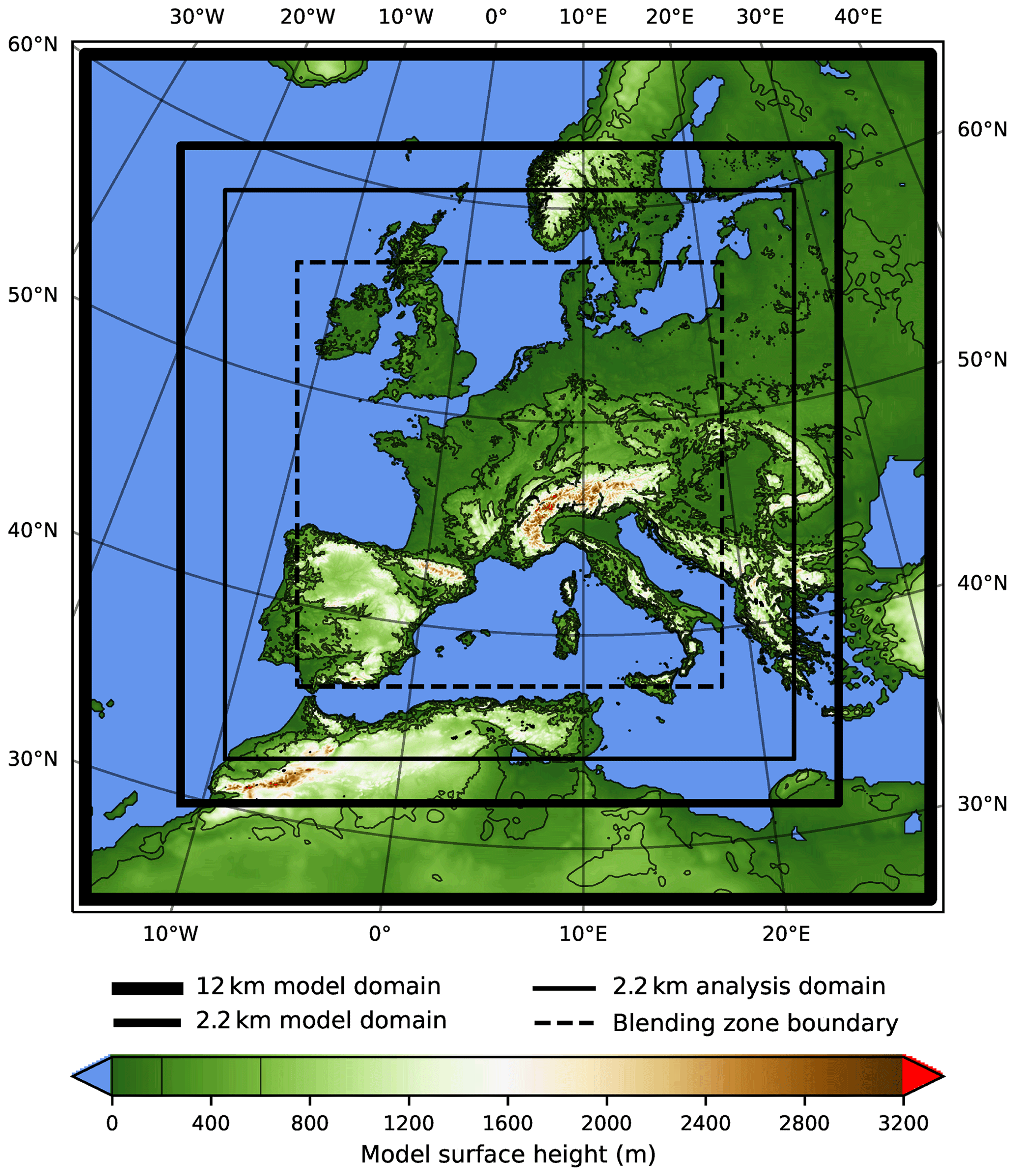
Figure 1Domain boundaries and model topography of the two COSMO simulations. The four black boxes show, from large to small, (bold) the model domain of the driving simulation with a horizontal grid spacing of 12 km, (semibold) the model domain of the nested simulation with a horizontal grid spacing of 2.2 km, (thin) the subdomain of the 2.2 km domain on which the precipitation attribution analysis is performed, and (dashed) the inner boundary of the blending zone that is used during the computation of the hybrid fields on which the feature identification is based (see Sect. 2.1). The model topography inside (outside) the 2.2 km domain boundary is that of the nested 2.2 km (driving 12 km) simulation.
In Sect. 2, we introduce the dataset and the methodology; in Sect. 3, we demonstrate our approach with two case studies; in Sect. 4, we present climatological results from the precipitation attribution; and in Sect. 5, we summarize the main findings.
2.1 Simulation and field preprocessing
We use hourly output from a 10-year regional climate simulation (1 January 1999 to 31 December 2008) with explicit deep convection over Europe, performed with a GPU-enabled prototype of the COSMO model (version 4.19; Fuhrer et al., 2014). A detailed description and evaluation of the simulation along with the detailed model setup can be found in Leutwyler et al. (2016, 2017) and Hentgen et al. (2019). We only analyze the 9-year period from 1 January 2000 to 31 December 2008 because not all fields necessary for our analysis have been archived during the first few months of the simulation. The domains of the nested COSMO simulations with 12 and 2.2 km grid spacing are shown in Fig. 1 together with the analysis domain of the high-resolution nest and the model topography. The analysis domain corresponds to the full computational domain minus 104 grid points (∼228.8 km) in each direction (those affected by the boundary relaxation). The orography differs between the driving ERA-Interim data, the 12 km simulation, and the 2.2 km simulation. While in response we expect significant local differences in precipitation, for instance in the vicinity of the Alps (see Heim et al., 2020, for a more thorough discussion), the larger-scale differences are expected to be small and locally confined as the simulation is still sufficiently constrained by the lateral boundary conditions. The COSMO simulation in the high-resolution nest with a horizontal grid spacing of 2.2 km has been performed on a grid. At the boundaries, it is driven by one-way nesting by a COSMO simulation with a horizontal grid spacing of 12 km on a grid. The domain of this coarser simulation is approximately 500 km larger in every direction than that of the nested simulation. In the 12 km simulation, deep convection is parameterized with an adapted version of the Tiedtke mass flux scheme (Tiedtke, 1989). The coarser COSMO simulation, in turn, is driven at the boundaries by global ERA-Interim reanalysis data available on a 1∘ grid every 6 h (Dee et al., 2011).
The high spatial resolution of the 2.2 km simulation presents some challenges for the objective identification of cyclones and fronts. While the domain of the 2.2 km simulation is large given its horizontal resolution, it is still relatively small with respect to these synoptic systems. This causes problems, for instance when a large-scale North Atlantic cyclone enters the domain from the west, because our algorithm cannot robustly identify cyclone features close to the boundaries, especially if their center (defined as the local pressure minimum) has yet to enter the domain. In addition, the high horizontal resolution can present challenges for our frontal identification algorithm, which is based on horizontal gradients (see below). From a technical perspective, the driving 12 km simulation thus at first glance appears to be more suitable to identify cyclones and fronts. However, this ignores that the fronts and cyclones are influenced by small-scale processes resolved in the nested 2.2 km simulation, as evidenced by their sometimes substantially different development in the two simulations in terms of their exact size and location – especially far downstream of the lateral boundaries, such as in the Mediterranean. These differences make it impossible to simply base the feature identification on the 12 km simulation. Instead, in order to exploit the advantages of both simulations, the 2.2 and 12 km data are merged in the following procedure:
-
Interpolate the 2.2 km fields to the part of the 12 km grid covered by the domain of the 2.2 km simulation.
-
In the interior of the domain at a distance of at least 50 coarse grid points (∼ 600 km) from the boundary of the 2.2 km domain (dashed box in Fig. 1), use these fields from the 2.2 km simulation.
-
Outside the 2.2 km domain, use the fields from the 12 km simulation.
-
In between (between the semibold and the dashed box in Fig. 1), blend the fields with , where x increases linearly from 0.0 at the inner boundary of the blending zone to 1.0 at the outer boundary, and f increases logistically in the same range, corresponding to the fraction of 12 km data.
The resulting hybrid fields possess the bigger domain and lower noise level of the 12 km simulation, which allows for a more robust feature identification over the analysis domain, especially close to the boundaries, such as over the North Atlantic. At the same time, they are meteorologically consistent with the 2.2 km simulation. We use the hybrid fields on the 12 km grid to identify cyclones (Sect. 2.2), fronts (Sect. 2.3), and high-pressure areas (Sect. 2.4) and then use the resulting feature masks at 2.2 km for the precipitation attribution analysis (Sect. 2.5).
2.2 Cyclones
The cyclone identification is based on the approach by Wernli and Schwierz (2006), who identified cyclones as two-dimensional features defined by closed sea-level pressure contours around local minima; the refinements by Sprenger et al. (2017); and the extension to multicenter cyclones by Hanley and Caballero (2012). For this study, the algorithm had to be adapted for limited-area domains. Additionally, in contrast to Wernli and Schwierz (2006) and Sprenger et al. (2017), tracking over time is based on the full two-dimensional extent of the features (see Appendix A) rather than only their center positions. As input fields, instead of sea-level pressure, we use geopotential (Φ) at 850 hPa for the sake of consistency with the fronts identified at that level. Seasonal feature and track frequency composites are provided in the Supplement (Figs. S1 and S2)
The Φ field is first smoothed with a Gaussian filter with a standard deviation σ=7 to eliminate spurious extrema on the high-resolution grid. In order to avoid artifacts, we exclude areas within two grid points (∼ 24 km) from the boundaries. Contours are then identified at an interval of 1 m2 s−2. Following Wernli and Schwierz (2006) and Sprenger et al. (2017), the outermost enclosing contour around each local minimum is detected by stepping through all enclosing contours until there is no further enclosing contour, the next contour also encloses a local maximum, or the next contour also encloses a fourth local minimum – the last criterion being a consequence of allowing up to three local minima per cyclone following Hanley and Caballero (2012). Two depth criteria are applied to eliminate spurious minima, whereby the depth of a cyclone feature corresponds to the difference in Φ between its lowest local minimum and its outermost enclosing contour (as determined by the criteria above). First, multicenter cyclone features that are too shallow are split into multiple single- or double-center cyclone features using the same approach (based on the relative depth of saddle points between minima) and thresholds as Hanley and Caballero (2012). Second, very shallow cyclone features with a total depth below 1 m2 s−2 are discarded.
The approaches by Wernli and Schwierz (2006), Sprenger et al. (2017), and Hanley and Caballero (2012) were developed for global datasets. Limited-area domains introduce an additional complication because it is impossible to determine whether contours that leave the domain are open or closed and/or whether they contain additional minima or maxima outside the domain. It is not obvious how to best deal with such boundary-crossing contours; there is a range of possible assumptions one may make. At one end is the assumption that all boundary-crossing contours are open, which immediately stops the growth of any cyclone feature that reaches the domain boundary. While this choice is safe, it severely limits the size of cyclones in the vicinity of the boundaries, which has effects far into the domain. At the other end is the assumption that all boundary-crossing contours are closed, which allows the cyclone features to continue growing uninhibited by the boundary. However, this often has the opposite effect, resulting in unreasonably large cyclone features in situations with a relatively flat pressure distribution. We opt for a compromise by allowing up to 20 % of the contours of a feature to be boundary-crossing. For example, if 16 closed contours are identified around a pressure minimum before the boundary is reached, then at most four additional boundary-crossing contours can be added before the 20 % threshold is reached at four out of 20 contours.
2.3 Fronts
The front identification approach is based on Jenkner et al. (2010) and involves multiple steps:
-
Compute fields of frontal strength and velocity.
-
Based on these, identify cold-frontal and warm-frontal areas as two-dimensional features.
-
Track these features over time.
-
Categorize the resulting front tracks as either synoptic or local.
The local fronts are then removed as only the synoptic fronts are used in this study. Seasonal feature and track frequency composites are provided in the Supplement (Figs. S1 and S2).
Fronts are characterized by strong horizontal contrasts in low-level temperature and humidity, which makes equivalent potential temperature θe at 850 hPa a suitable field for front detection (specifically, the modulus |∇θe| of the θe gradient). Schemm et al. (2018) discuss this choice in detail and provide a historical context. Following the general approach proposed by Hewson (1998), the front identification method developed by Jenkner et al. (2010) is based on applying the thermal front parameter (TFP; Renard and Clarke, 1965) to θe and using the cross-frontal wind component to distinguish between cold, warm, and quasistationary fronts.
The frontal areas are derived from a thermal and a wind component:
-
The thermal component is based on θe at 850 hPa. The θe field is first smoothed with the diffusive filter described by Jenkner et al. (2010) with 25 repetitions. Then a mask is derived from its absolute gradient |∇θe| by applying a minimum threshold, which varies over the year to account for the strong seasonal cycle of humidity (and therefore of θe) that leads to substantially lower cross-frontal θe gradients in winter than in summer and thus far fewer winter than summer fronts for a given threshold (Rüdisühli, 2018). A |∇θe| threshold value is defined in the middle of each month (Table 1) and linearly interpolated to each hour in-between.
-
The wind component is based on frontal velocity vf at 850 hPa,
where v is the horizontal wind vector, and TFP denotes the thermal front parameter, defined as
A mask is derived with |vf| ≥ 1 m s−1.
Table 1Midmonthly |∇θe| threshold values in kelvin per 100 km to compute the thermal component of frontal areas, as described in Sect. 2.3.

The frontal areas correspond to the overlap between the thermal and the wind component masks. The sign of vf determines whether an area is classified as cold-frontal () or warm-frontal ().
In a next step, the frontal features are tracked over time using the tool described in Appendix A. Cold-frontal and warm-frontal features are tracked separately. A minimum lifetime criterion of 24 h is applied to discard short-lived fronts. The resulting front tracks are then grouped into synoptic and local fronts based on track properties. Synoptic fronts are generally larger and more mobile (i.e., less stationary) than local fronts, which are largely produced by differential heating along topography and coasts. These properties can be expressed by a pair of criteria (on which we have settled after extensive manual testing):
-
The typical feature size of a track is calculated by first combining, at each time step, the sizes of all features that belong to the track and then calculating the 80th percentile of these total sizes over all time steps. Front tracks are only considered synoptic if the typical feature size is at least 400 grid points (∼2000 km2).
-
The stationarity of a track is determined as the typical feature size divided by the total footprint area (defined by all grid points that belong to the tracked front at any time). Front tracks are only considered synoptic if the stationarity is below .
All tracks fulfilling both criteria are considered synoptic fronts and thus both large and mobile. All remaining tracks are considered local fronts and thus small and/or stationary. Only synoptic fronts are used for the precipitation attribution analysis, while local fronts are removed.
2.4 High-pressure areas
Precipitation not only occurs near cyclones and fronts but also in areas of weak synoptic forcing that are typically characterized by relatively high pressure and a flat pressure distribution, for example diurnal summer convection over the continent. When attributing precipitation only to cyclones and fronts, such precipitation would not be captured but instead be part of the residual. Our original method without high-pressure areas, however, often misclassified diurnal summer convection as front-related (specifically far-frontal, as defined in Sect. 2.5). To prevent this, we first exclude precipitation in such areas characterized by high-pressure and a flat pressure distribution (henceforth simply called high-pressure areas), which we identify based on the geopotential Φ and its gradient ∇Φ at 850 hPa. Seasonal frequency fields of the identified high-pressure areas are provided in the Supplement (Fig. S1).
Computing the high-pressure areas (at 850 hPa) involves the following steps:
-
Smooth the Φ field using a Gaussian filter with a standard deviation of σ=3. Then compute a Φ mask covering areas with high pressure based on a minimum threshold which varies over the year to account for the seasonal cycle in Φ. The threshold at a given time step is derived by linear interpolation from the midmonthly values listed in Table 2.
-
Smooth the Φ field again using a Gaussian filter with a standard deviation of σ=20, then compute ∇Φ, whereby the gradient at each grid point is computed across multiple unit grid distances using offsets of , corresponding to ±120 km in our hybrid 12 km fields. Then compute a ∇Φ mask covering areas with a weak pressure gradient based on a constant maximum threshold of 0.02 m s−2.
-
The high-pressure area corresponds to the overlap area of the Φ and ∇Φ masks.
Table 2Midmonthly Φ threshold values in square meters per second squared to compute the Φ component of high-pressure areas at 850 hPa, as described in Sect. 2.4.

All threshold values have been determined subjectively based on extensive manual evaluation of multiple years of data. In contrast to cyclones and fronts, high-pressure areas are not tracked over time.
2.5 Front–cyclone-relative components
In order to attribute precipitation to fronts and cyclones, we decompose the domain at each time step into seven so-called front–cyclone-relative components, as illustrated in Fig. 2. They are mutually exclusive and defined in the following order, where each grid point is assigned to the first component whose criteria it fulfills:
-
The high-pressure component comprises all grid points within a high-pressure area mask, regardless of the presence of any fronts or cyclones. Its purpose is to capture precipitation in areas of weak synoptic forcing such as diurnal summer convection over the continent. Applying this criterion first, before all others, prevents spurious front features – frequent in the Mediterranean in summer – from capturing diurnal summer convection precipitation as far-frontal.
-
The cyclonic component comprises all remaining grid points within a cyclone mask, regardless of the presence of any fronts. Its purpose is to capture precipitation produced close to the center of cyclones.
-
The cold-frontal component comprises all remaining grid points within 300 km of a cold-frontal feature but farther than 300 km from any warm-frontal feature. Its purpose is to capture all precipitation produced close to cold fronts but in relative isolation from the influence of warm fronts and cyclone centers.
-
The warm-frontal component is analogous to the cold-frontal component but for warm fronts.
-
The collocated component comprises all remaining grid points within 300 km of both a cold-frontal and a warm-frontal feature. Its purpose is to capture precipitation simultaneously influenced by cold and warm fronts but away from cyclone centers, for instance, areas near a frontal fracture or frontal occlusion. In addition, it also occasionally captures strong warm conveyor belts because their eastern boundary can be associated with a band of very high θe that is identified as a warm front located within 300 km ahead of the cold front.
-
The far-frontal component comprises all remaining grid points within 300–600 km of a front of either type. No distinction is made between cold and warm fronts in order to keep the number of groups reasonably small. Its purpose is to capture precipitation more remotely related to yet still influenced by fronts.
-
The residual component comprises all remaining grid points. Its purpose is to capture precipitation that our approach cannot attribute to a specific weather system. Under the assumption that the other six components capture the major sources of precipitation, we expect the residual contributions to be comparatively small.
The thresholds that define the near-frontal (300 km) and far-frontal (600 km) components have been chosen subjectively based on our best judgment while studying a wide range of cases.

Figure 2Schematic depiction of the seven front–cyclone-relative components (as defined in Sect. 2.5): high-pressure, cyclonic, cold-frontal, warm-frontal, collocated, far-frontal, and residual. Note that they are mutually exclusive and cover the whole domain; i.e., at a given time step, each grid point is assigned to exactly one component.
In order to illustrate our approach, we present two case studies: one of a winter and one of a summer cyclone.
3.1 Winter Cyclone Lancelot
Winter storm Lancelot (FU Berlin, 2007a) affected Europe during 19–21 January 2007 in the wake of well-known winter storm Kyrill (see Leutwyler et al. (2015) for an animation based on the same simulation that includes both storms).
3.1.1 Development
At 00:00 UTC on 20 January 2007 (Fig. 3a) the cyclone center approaches Ireland, accompanied by a warm front extending southeastward into the North Sea and central Europe and a cold front extending southwestward across the British Isles into the North Atlantic. A large area of precipitation associated with the warm front extends over the North Sea to the rear of the cyclone center. A smaller band of precipitation accompanies the cold front, separated from the warm-frontal precipitation area by a dry gap region.
At 12:00 UTC on 20 January 2007 (Fig. 3b), the cyclone center has almost completely crossed the North Sea and is approaching the southern tip of Norway. The cold front has been moving away from the cyclone center toward the southeast. It is oriented at a right angle to the warm front, forming a frontal T-bone typical of Shapiro–Keyser-type cyclones (Shapiro and Keyser, 1990). Along the cold front, oval-shaped precipitation cores are discernible, which are oriented at a slight clockwise angle relative to the front and separated by gap regions, reminiscent of a narrow cold-frontal rainband. In the cold sector behind the cyclone there is widespread patchy precipitation, some of it associated with a relatively shallow cyclone near the British Isles in a way reminiscent of secondary cold-frontal lines as described, for instance, by Browning et al. (1997).
At 00:00 UTC on 21 January 2007 (Fig. 3c), the cyclone center resides over the southern Scandinavian Peninsula. The warm front has moved across the southern Baltic Sea while still producing precipitation over an extended area. The cold front, by now far away from the cyclone center, has moved over continental Europe, extending from the North Atlantic near the northern tip of Iberia across France and Germany into eastern Europe. It is oriented roughly parallel to the Alpine crest, which it steadily approaches. The eastern part of the cold front over Germany and eastern Europe has started to disintegrate.
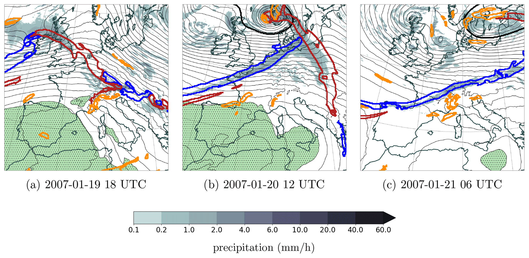
Figure 3Development of Cyclone Lancelot in January 2007. Thin black contours indicate the geopotential at 850 hPa, gray shading the surface precipitation, and green stippling the high-pressure areas. Bold contours represent the outlines of tracked features: synoptic cold and warm fronts (blue and red), local fronts of either type (orange), and cyclones (black).
3.1.2 Precipitation attribution
Figure 4 shows the attribution to fronts and cyclones of the precipitation accumulated during the 3 d when Cyclone Lancelot affected Europe. Total accumulated precipitation is distributed across most of the northern half of the domain, with a pronounced local maximum along the northern flank of the Alps (Fig. 4a). In addition, local maxima occur over and west of Scotland, over southern Norway, and to a lesser degree over Denmark and along the Baltic coast. The Mediterranean is dry. Most components contribute at least some precipitation, with the exception of high-pressure areas (Fig. 4e). A lot of precipitation is classified as frontal, with cold-frontal precipitation mainly north of the Alps (Fig. 4b), warm-frontal precipitation covering an elongated region extending from the North Sea across Denmark into Poland (Fig. 4c), and large amounts of collocated precipitation distributed in two distinct band-like regions farther south and north (Fig. 4d). The precipitation maximum along the Alps is identified as primarily collocated; however, it largely predates the passage of Lancelot and is at least partially caused by remnants of Kyrill (the cyclone system immediately preceding Lancelot), as is evident from Fig. 3a. Also attributable is some cyclonic precipitation over southern Scandinavia and the Baltic (Fig. 4f) along with some scattered far-frontal precipitation (Fig. 4g). Residual precipitation is largely restricted to the northern part of the British Isles and the adjacent North Atlantic (Fig. 4h). As Fig. 3b, c indicate, postfrontal precipitation was largely responsible for the residual, partly organized in secondary frontal and cyclonic structures not identified as synoptic features.
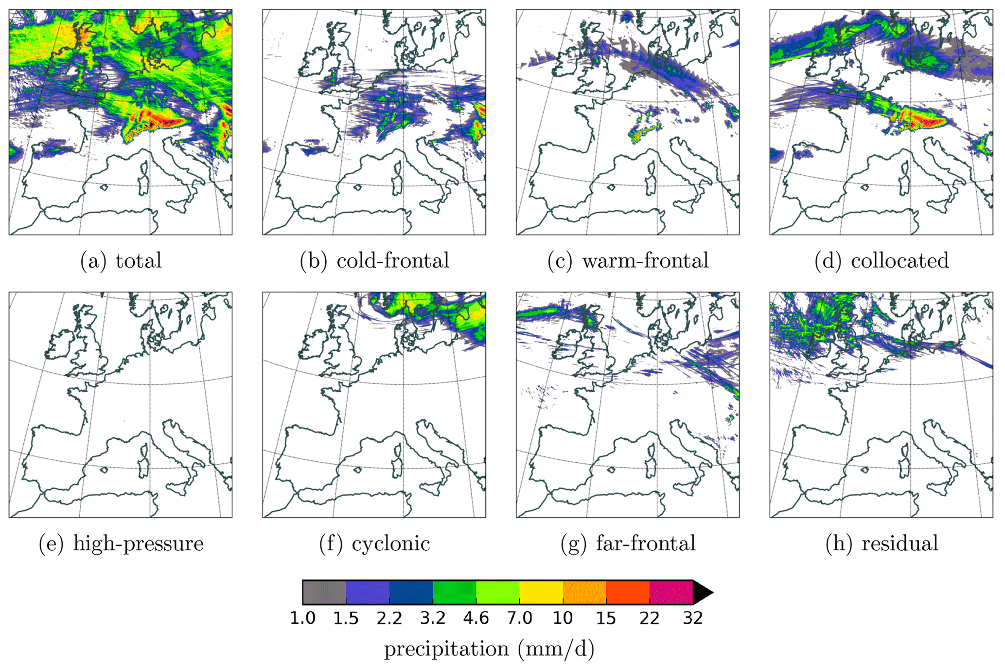
Figure 4Front–cyclone-relative precipitation contributions to Cyclone Lancelot during the 3 d period 19–21 January 2007.
3.2 Summer Cyclone Uriah
In late June 2007, Cyclone Uriah (FU Berlin, 2007b) moved across the British Isles and the North Sea accompanied by a strong cold front and a weak warm front.
3.2.1 Development
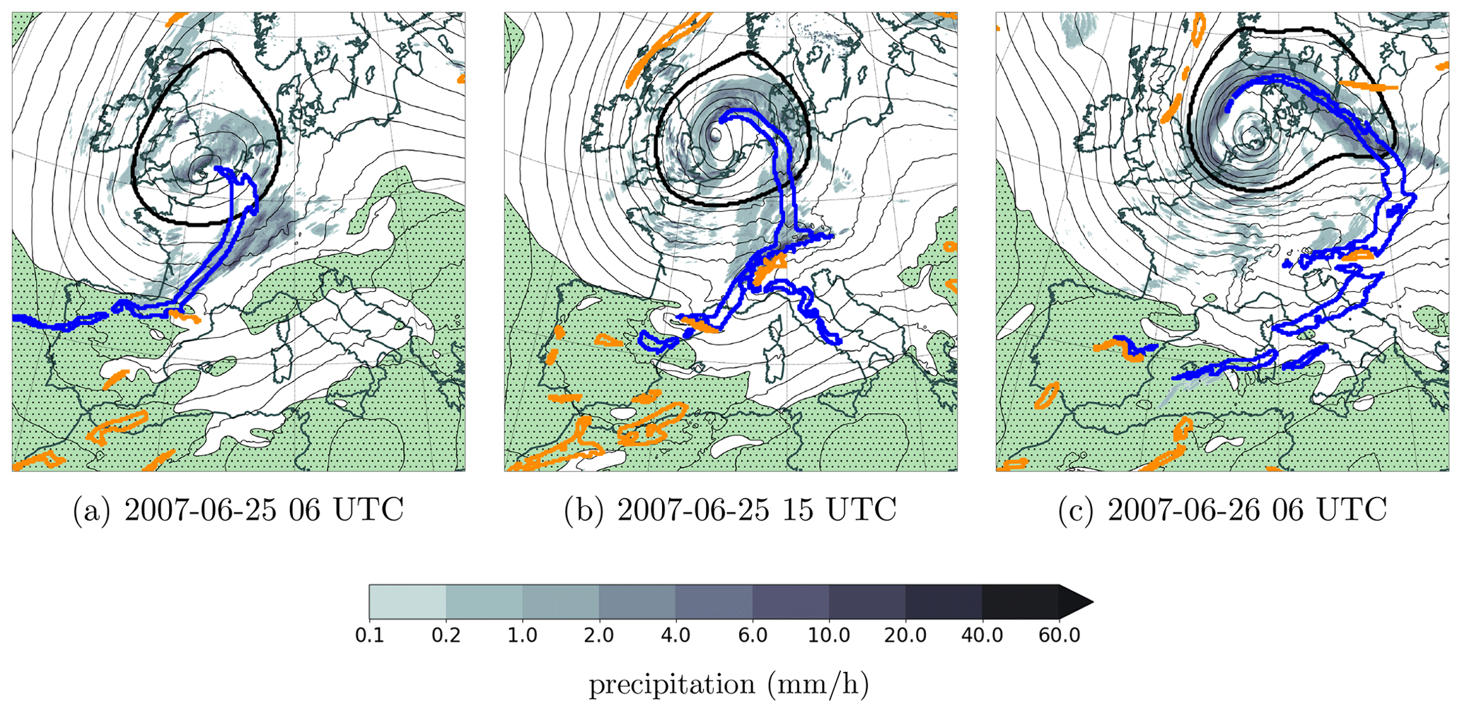
At 06:00 UTC on 25 June 2007 (Fig. 5a), the cold front is part of a baroclinic zone that extends from northeastern France southwestward to Gibraltar. The main precipitation areas are located just north of the cyclone center as well as along and ahead of the cold front over France and Germany. East of the cyclone center, a weaker warm-frontal zone (discernible from meteorological fields, which are not all shown) extends into eastern Europe, but at this point it is not yet recognized as a frontal feature. Northwest of the cyclone center, cold and dry air is advected southward. The southern boundary of this cold zone constitutes a weakly precipitating cold front that approaches the British Isles.
At 15:00 UTC on 25 June 2007 (Fig. 5b), the main cold front is gaining strength while moving over France and Germany. Its northern end has started to wrap around the cyclone center and produces substantial precipitation, while its southern end has reached the Alps, producing strong precipitation along the northern Alpine flank. Behind the cold front, over France many isolated cells produce fragmented precipitation of weak to moderate intensity. The warm front east of the cyclone is much weaker than the cold front and only produces some precipitation close to the cold front, where occlusion may have commenced. It has still not been identified as a feature by the algorithm. The baroclinic zone southwest of the cyclone center has been fragmented while moving over Iberia and France. The minor cold front to the northwest of the cyclone center has reached Scotland and Ireland while falling dry.
At 06:00 UTC on 26 June 2007 (Fig. 5c), the main cold front has moved from Germany over eastern Europe and southern Scandinavia. It is mostly oriented northwest–southeastward, except for its northern end, which is bent around the cyclone center. Precipitation is still substantial along most of the front. The precipitation band along its bent-back portion wraps almost completely around the cyclone center, much farther than the corresponding front feature, which suggests that a part of the front has not been detected as a feature by our algorithm. The southern end of the cold front has been held back along the Alps, but orographic precipitation there has largely stopped. In the cold sector behind the front, over France and Germany, fragmented postfrontal precipitation is still prevalent. By now, the weak warm front has been detected as a feature but merely as a local front, which is not used for the precipitation attribution. Along most of its length, the warm front has been caught up by the cold front, suggesting occlusion. The baroclinic zone consisting of many small frontal fragments has crossed the Spanish and French coast into the Mediterranean. The minor cold front over Great Britain at the boundary of the cold zone has stopped precipitating and is now followed by a pair of likewise dry warm fronts along the western border of the cold zone.
3.2.2 Precipitation attribution
Figure 6 shows the attribution to fronts and cyclones of the precipitation accumulated during the 4 d when Cyclone Uriah affected Europe. In contrast to Lancelot (Sect. 3.1) – a fast-moving cyclone accompanied by a pronounced warm front and an extended cold front – Uriah constituted a slow-moving cyclone accompanied by a pronounced cold front but no discernible warm front. The precipitation attribution is entirely consistent with that characterization. Most accumulated precipitation is concentrated in a ring-shaped area centered on the Danish straits, with maxima over the North Sea and southern Sweden (Fig. 6a). The precipitation area extends over the British Isles and France to the west and southwest and southward to the Alps, along the northern flank of which precipitation amounts are locally enhanced. Southern Europe and the Mediterranean are entirely dry. Most precipitation is classified as either cyclonic (Fig. 6f) – mainly over the North Sea, southern Scandinavia, and the Baltic Sea – or cold-frontal, mainly over Germany and Poland near the Baltic coast and extending southwestward to the Alps (Fig. 6a). While there is also some far-frontal and residual precipitation (Fig. 6g, h), there is essentially no warm-frontal, collocated, or high-pressure precipitation (Fig. 6c, d, e).
These case studies illustrate that our method is able to attribute precipitation to cyclones and fronts meaningfully and to capture the large case-to-case variability of the various contributions.

Figure 6As in Fig. 4 but for Cyclone Uriah during the 4 d period 24–27 June 2007.
In this section, the 9-year (2000–2008) climatology of precipitation and its link to the features in Fig. 2 are discussed. First, we consider total precipitation in Sect. 4.1, whereby the annual and seasonal climatologies are discussed separately. Then, we focus on heavy precipitation in Sect. 4.2.
4.1 Total precipitation
The main results of the total precipitation attribution are shown in Fig. 7 for absolute annual-mean amounts, Fig. 8 for absolute seasonal-mean amounts, and Fig. 9 for relative seasonal-mean contributions. In the annual mean, the amounts of total precipitation are generally larger in the northern part of the domain than in the Mediterranean. The largest amounts, however, occur over modest to high topography, especially the Alps, the Dinaric Alps, the Scandinavian Mountains, the Scottish Highlands, and the Pyrenees. In the North Atlantic, the precipitation amounts decrease from north-northwest toward south-southeast. With respect to the front–cyclone-relative contributions, several interesting features are discernible: (i) cold-frontal precipitation amounts are largest over the Alps and still large to the north-northwest thereof but rather small in the Mediterranean and the Baltic Sea; (ii) large warm-frontal amounts are found over the North Atlantic and (to a lesser degree) over central Europe but almost none in the Mediterranean; (iii) cyclonic precipitation is relatively uniformly distributed across the domain, with peak values in the North Atlantic, over the British Isles and northern Scandinavia, and in the Mediterranean, which makes it the only component that contributes substantially to Mediterranean precipitation; (iv) the amounts of high-pressure precipitation are large along a continental band extending from the Pyrenees to the Alps and the Dinaric Alps, with another band extending along the Apennines; and (v) the residual precipitation (i.e., the amounts that cannot be attributed to any front–cyclone-relative component) is relatively evenly distributed across the domain, with enhanced values only over the Alps and the Scandinavian Mountains.
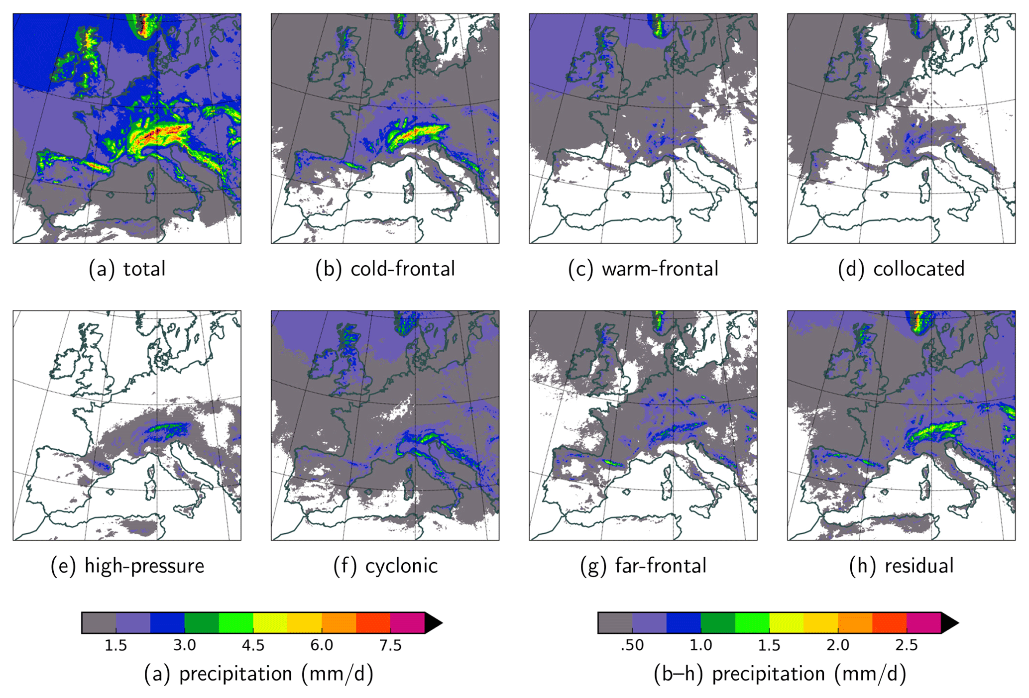
Figure 7Mean daily precipitation during the 9-year period 2000–2008 (a) overall and (b–h) separated into seven front–cyclone-relative contributions.
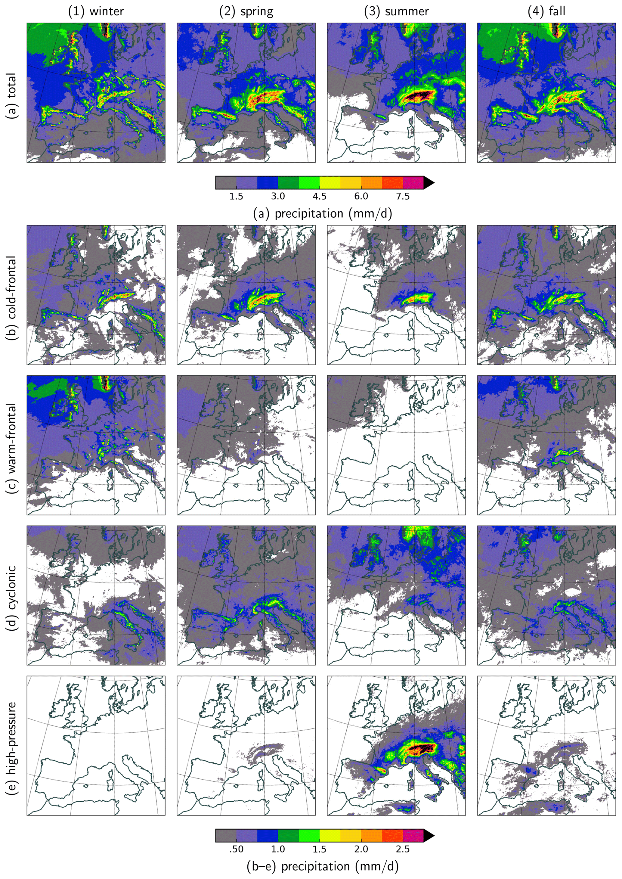
Figure 8Mean daily precipitation during (1–4) each season of the 9-year period 2000–2008 (a) overall and (b–e) of selected front–cyclone-relative contributions.
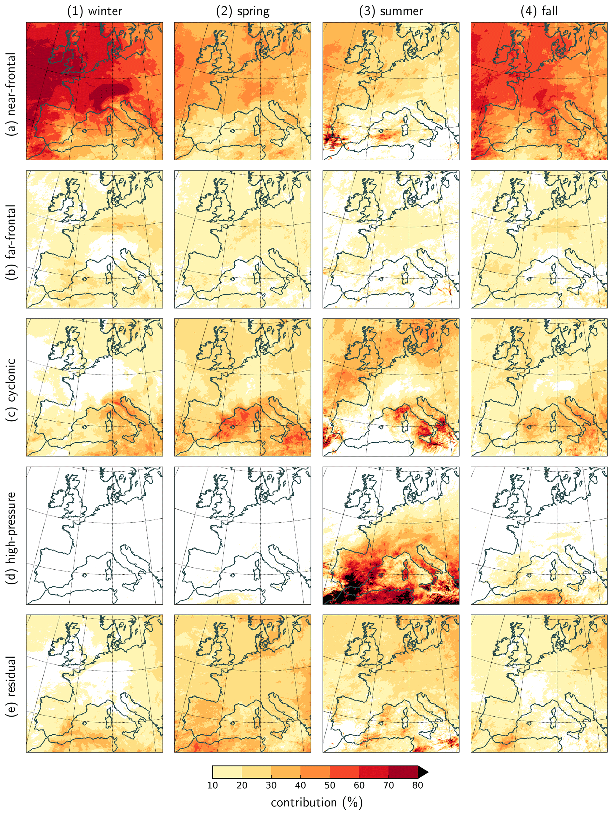
Figure 9Relative precipitation contributions during (1–4) each season of the 9-year period 2000–2008 of front–cyclone-relative components: (a) sum of cold-frontal, warm-frontal, and collocated; (b) far-frontal; (c) cyclonic; (d) high-pressure; and (e) residual.
The discussion so far has ignored the fact that there are significant seasonal variations (Fig. 8). In winter, total precipitation is shifted from the continental regions to the North Atlantic. In spring, the distribution is similar as in the annual mean, except for slightly below-average amounts in the North Atlantic, the Baltic, and the Mediterranean Sea, with slightly more precipitation over the Alps, the Pyrenees, and the Dinaric Alps. In summer, the spatial distribution across the domain is the least uniform among all seasons: the Mediterranean Sea and the Iberian Peninsula are almost completely dry, while most of continental Europe receives more precipitation than on average, and the contrast between the large precipitation amounts over the Alps and the dryer surrounding areas is more pronounced than in any other season. Furthermore, during summer, no peak amounts are discernible over the Pyrenees and the Dinaric Alps, quite in contrast to spring and fall. Finally, the precipitation in fall is similarly distributed as in the annual mean, except for larger precipitation amounts in the North Atlantic relative to continental Europe. Peak amounts in fall occur over the Alps, the Scandinavian Mountains, the Pyrenees, the Dinaric Alps, and the Scottish Highlands, as they do in the annual mean.
Like for the amounts and geographical distribution of total precipitation, seasonal variations can also be expected for the front–cyclone-relative components. Physically, this is of course based on the seasonal cycle of the considered weather features (cold and warm fronts, cyclones, high-pressure areas). For instance, it is well known that Alpine lee cyclones form preferentially during spring and fall in the Gulf of Genoa (e.g., Campins et al., 2011) and that North Atlantic cyclones, with their accompanying cold and warm fronts, affect continental Europe more often in winter than in summer (e.g., Hénin et al., 2019). Seasonal variations in front–cyclone-relative precipitation amounts must, therefore, be expected and interpreted with respect to the corresponding shifts in the weather features. In the Supplement, we provide seasonal climatologies of fronts, cyclones, and high-pressure areas (Figs. S1 and S2) along with the occurrence and wet-hour frequencies of the front–cyclone-relative components (Figs. S3–S6). Here, we restrict the discussion to a few selected seasonal effects on the relative precipitation amounts: (i) cold-frontal precipitation is more uniformly distributed across the domain in winter and fall than in spring and summer, whereby in summer, cold-frontal precipitation is mostly restricted to the continent, specifically western, eastern, and northern Europe; (ii) warm-frontal winter precipitation is similarly distributed as the annual mean – with peak values over the North Atlantic and the British Isles and somewhat smaller values over central Europe – whereas summer warm-frontal precipitation is nearly nonexistent over the continent; (iii) the amounts of cyclonic winter precipitation are below the annual mean over continental Europe and the North Atlantic but above-average in the Mediterranean, especially in the Adriatic and Tyrrhenian seas and over the Apennines, in contrast to summer, with nearly no cyclonic precipitation over the Mediterranean Sea; and (iv) high-pressure precipitation dominates in summer over much of western and southeastern Europe, whereas it is completely missing during winter and only weakly discernible in spring and fall. This short list, of course, can only provide a glimpse of the many local seasonal effects. Furthermore, as mentioned before, we did not show and describe the seasonality of the collocated and far-frontal components, which, however, can be found in the Supplement (Figs. S3–S6).
Instead of analyzing in greater detail the absolute precipitation amounts and how they can be attributed to the front–cyclone-relative components, we now consider the relative contributions by addressing the questions what percentage of the total precipitation can be attributed to the main components of a front–cyclone system and what percentage is attributable to either the high-pressure or residual components. The results are shown in Fig. 9, split according to season and for the components: near-frontal (i.e., cold-frontal, warm-frontal, or collocated), cyclonic, far-frontal, high-pressure, and residual. Several noteworthy patterns are discernible. During winter and fall, a substantial percentage of the total precipitation occurs close to fronts over the North Atlantic and central Europe (up to >70 % in winter, about 60 % in fall), and to a lesser degree the Mediterranean (up to >50 %). Far-frontal precipitation is neither as prevalent nor as variable, with 10 %–20 % in most areas year-round. Cyclonic and far-frontal percentages are largest in the Mediterranean, particularly in spring (regionally up to 50 %). High-pressure percentages are negligible except for summer, when the contribution exceeds 70 % over the Iberian Peninsula, middle to southern Italy, and Sardinia and Corsica. As expected, part of the total precipitation cannot be attributed to any of the components. The relative residual contributions are rather uniform, both in time and in space. In spring, they reach about 25 %. Over central Europe and the North Atlantic, including the British Isles, the residual percentages are still smaller, at about 10 %, especially in winter and fall.
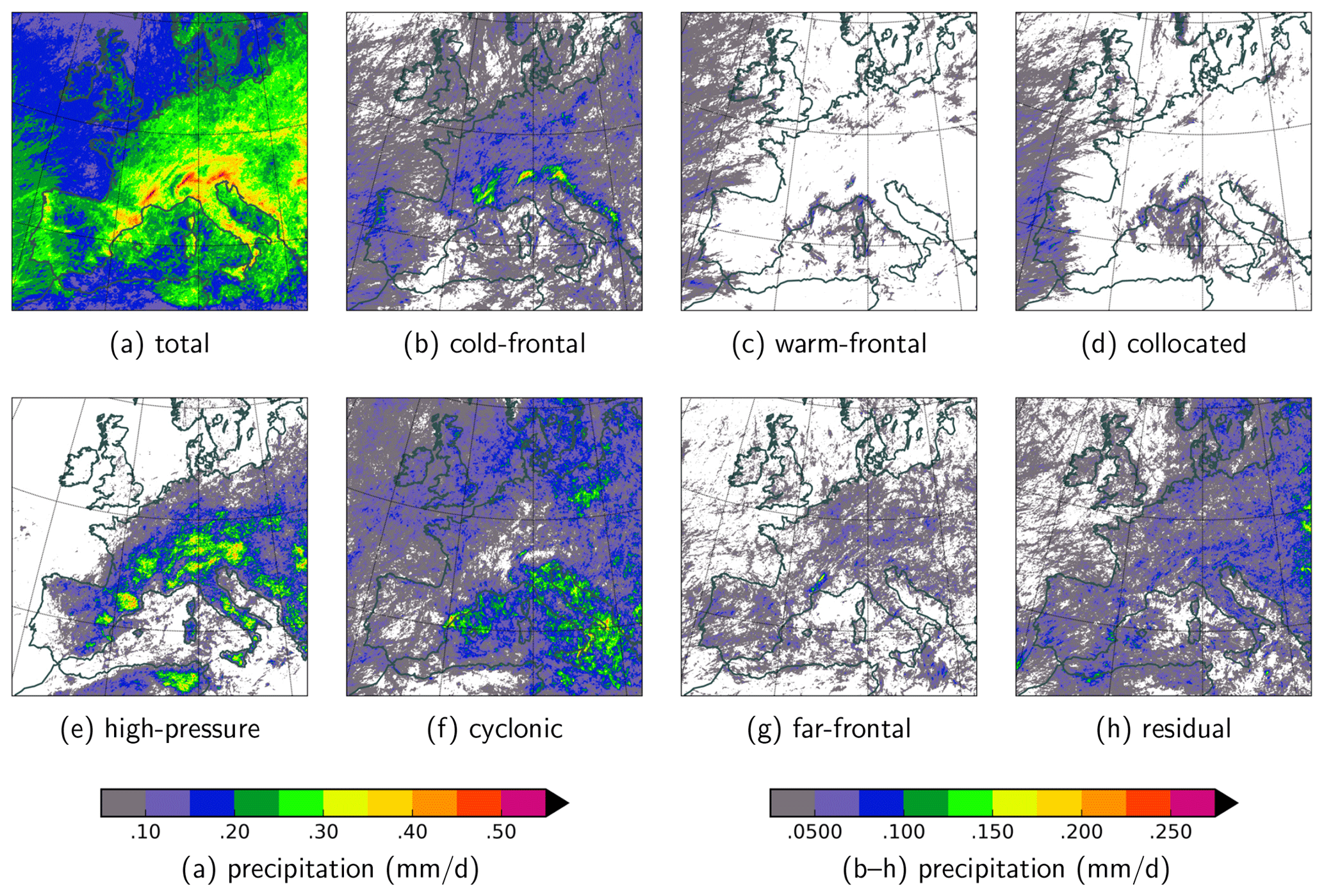
Figure 10Like Fig. 7 but for annual heavy precipitation, defined as the amount exceeding the local 99.9th all-hour percentile of hourly precipitation intensity over the whole year.
4.2 Heavy precipitation
After the discussion of total precipitation in the previous section, we now shift our focus to heavy precipitation. It is defined as the amount of precipitation exceeding the local (i.e., grid-point-specific) 99.9th all-hour percentile of hourly precipitation intensity (i.e., including dry hours, as recommended by Schär et al., 2016), corresponding to a return period of about 1.4 months. Separate thresholds are computed for annual and seasonal analyses, respectively.
The spatial distribution of annual-mean heavy precipitation (Fig. 10a) differs from that of total precipitation (Fig. 7) in that the former preferentially occurs over land and in that heavy precipitation amounts in the Mediterranean are similar to those over continental Europe and larger than those in the North Atlantic. While total precipitation exhibits the strongest spatial gradients from low to high topography, especially in the Alpine region, heavy precipitation shows a more pronounced land–sea contrast, especially between the North Atlantic and continental Europe. Local maxima in amounts of heavy precipitation occur over high topography along the northern Mediterranean, specifically over the Alps, the Pyrenees, the Dinaric Alps along the Balkan coast, and the Apennines.

Figure 11Like Fig. 8 but for seasonal heavy precipitation, defined as the amount exceeding the local 99.9th all-hour percentile of hourly precipitation intensity in a given season.
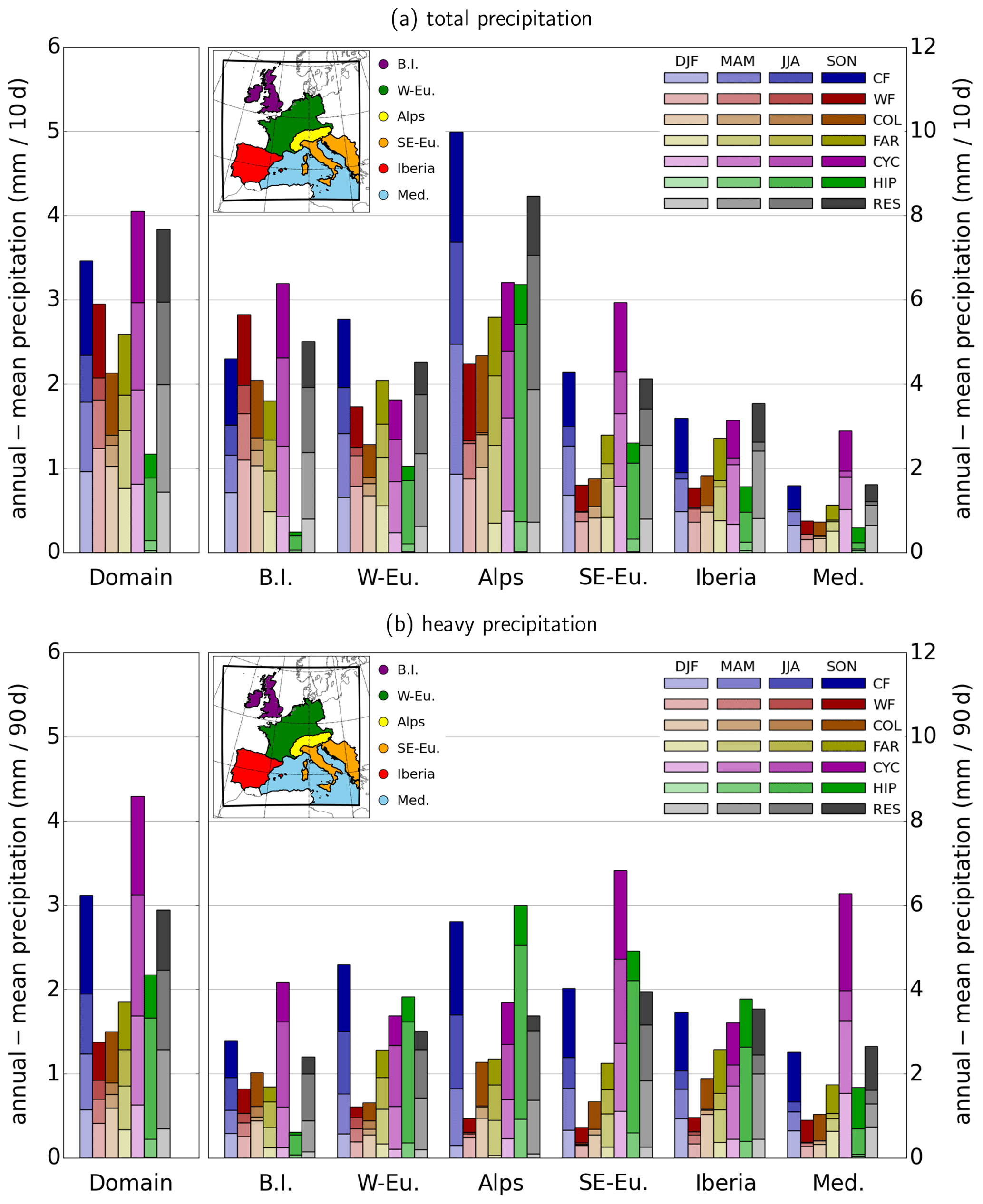
Figure 12Mean (a) total and (b) heavy precipitation over the analysis domain and six selected regions, as indicated in the map: British Isles, western Europe, Alps, southeastern Europe, Iberia, and the Mediterranean Sea. Heavy precipitation is defined as the amount of hourly precipitation above the local (grid-point specific) seasonal 99.9th all-hour percentile. Each bar shows the annual-mean precipitation contribution of one front–cyclone-relative component (CF: cold-frontal; WF: warm-frontal; COL: collocated; FAR: far-frontal; CYC: cyclonic; HIP: high-pressure; RES: residual), with the four segments indicating the relative contribution of each season (DJF: winter; MAM: spring; JJA: summer; SON: fall). To obtain approximate absolute seasonal-mean amounts, multiply the height of a bar segment by four. Note that there is no relation between the colors of the bars and those of the regions on the map.
The front–cyclone-relative components of annual-mean heavy precipitation can be sorted into two groups: (i) cold-frontal, high-pressure, cyclonic, and residual precipitation (Fig. 10b, e, f, h), which each contribute substantial amounts of heavy precipitation in specific areas, and (ii) warm-frontal, collocated, and far-frontal heavy precipitation contributions (Fig. 10c, d, g), which are much smaller and are therefore not discussed any further. Some specific attribution results with respect to the first group are that (i) cold-frontal heavy precipitation (Fig. 10b) occurs in large amounts over and around the Alps as well as along the Balkan and the northwestern Iberian coasts; (ii) high-pressure heavy precipitation (Fig. 10e) is restricted to continental areas (both Europe and northern Africa) and contributes by far the largest share of heavy precipitation over land; (iii) cyclonic heavy precipitation (Fig. 10f) resembles cyclonic total precipitation in its relatively even spatial distribution and only weak local enhancement over high topography, while contributing almost all heavy precipitation over the Mediterranean Sea and, to a lesser degree, in the North Atlantic and the North Sea; and (iv) amounts of residual heavy precipitation (Fig. 10h) tend to be larger over land than over sea and to increase toward eastern Europe, albeit – in contrast to total precipitation – without any local enhancement over high topography.
Like total precipitation, heavy precipitation exhibits seasonal variations in both geographical distribution and front–cyclone-relative attribution. The clear separation into the two abovementioned groups in the annual mean disappears at the seasonal level, which reflects the fact that different mechanisms are responsible for heavy precipitation in different seasons, which is expected given the seasonality of the considered weather features (see Figs. S1 and S2). Heavy winter precipitation (Fig. 11a) is more prevalent over sea than over land – in contrast to the annual mean – with the largest amounts over the Mediterranean Sea (and especially the Ionian Sea) as well as along the Iberian west coast. In spring, heavy precipitation (Fig. 11a) exhibits a pronounced land–sea contrast, with large amounts distributed evenly across continental Europe and local maxima over the Alps and the Tunisian Atlas mountains. Compared with winter, this corresponds to a pronounced north- and landward shift of heavy precipitation in the southern part of the domain. No season experiences more heavy precipitation than summer (Fig. 11a), the season when the northward shift since winter peaks. Amounts of heavy precipitation are large over all of continental Europe except Iberia, with peaks over the Alps, and moderate further north, over the British Isles, the Baltic, and the North Atlantic. Meanwhile, the Mediterranean Sea and southern Iberia are almost dry. The onset of fall is accompanied by a southward shift of heavy precipitation from continental Europe to the Mediterranean (Fig. 11a). The spatial distribution is almost mirrored with respect to summer, with most heavy precipitation in the previously dry Mediterranean and Iberia, while the land–sea contrast along the rest of the North Atlantic coast completely disappears. Italy and the Balkan coast are the only extended regions where heavy precipitation is prevalent in both summer and fall. By far the largest amounts of heavy precipitation occur along the coasts of France and Spain, from the Gulf of Lion to the Balearic Sea, along with secondary hot spots in the Tyrrhenian and Ionian seas.
Heavy precipitation is attributable to different processes in different seasons (Fig. 11), same as we have already shown for total precipitation (Fig. 8): (i) the main areas of heavy winter precipitation in the Ionian Sea and along the western Iberian coast originate primarily from cyclones (Fig. 11d) and fronts (especially cold fronts; Fig. 11b, c), respectively; (ii) similarly, the cyclonic component (Fig. 11d) is the primary source of heavy precipitation in the Mediterranean in the other seasons, especially in fall, and over northern Europe and the North Atlantic in summer; (iii) the widespread occurrence of heavy summer precipitation over the continent almost entirely coincides with high-pressure areas (Fig. 11e), which on the other hand are completely irrelevant in winter; and (iv) while cold fronts (Fig. 11b) steadily contribute heavy precipitation over the continent from spring through fall, with peak contributions along the northwestern Mediterranean coast (Gulf of Lion, Gulf of Genoa) in fall, warm fronts (Fig. 11c) are mostly irrelevant for heavy precipitation.
Complementary to this discussion of the absolute front–cyclone-relative contributions to heavy precipitation, the relative contributions of a subset of the components are provided in the Supplement (Fig. S7).
Hourly fields from a kilometer-scale regional climate simulation for present-day climate conditions over Europe, covering the 9-year period 2000–2008, have been used to perform a detailed climatological attribution of total and heavy precipitation to a set of synoptic weather systems: cyclones, cold and warm fronts, high-pressure areas (capturing diurnal summer convection), and derived categories (regions with collocated cold and warm fronts and far-frontal regions). To the best of our knowledge, this is so far the most detailed synoptic feature attribution exercise for European precipitation, which led to important findings related to both methodological and meteorological aspects. First, the attribution has been applied to two storms passing over Europe: the winter Cyclone Lancelot (19–21 January 2007) and the summer Cyclone Uriah (24–26 June 2007). Based on these two case studies and further refined in the 2000–2008 climatological analysis, the methodological key aspects can be summarized as follows:
-
Although fairly established algorithms existed for automatically identifying cyclones and fronts in comparatively coarse reanalysis and global climate simulation data, their application required great efforts in testing and adjusting for use with kilometer-scale simulation output (e.g., by increasing spatial smoothing and by introducing additional criteria). These efforts can hardly be automated, and the thresholds finally used are not universal; i.e., they would need further adjustment if considering a different region, climate model, or resolution. The final setup of our algorithms should not be regarded as perfect but rather pragmatically as one out of potentially several meaningful options.
-
A large model domain is required in order to meaningfully identify frontal cyclones, in particular in the North Atlantic storm track region. Although, compared with previous kilometer-scale climate simulations, our simulation was performed on a huge domain, it was essential to perform the identification of cyclones and fronts on the even larger domain of the driving coarser model (using hybrid fields based on both simulations). Only with this spatial extension did the robust identification of North Atlantic cyclones and their sometimes elongated trailing fronts approaching Europe become possible.
-
A particular challenge related to the front identification is the choice of the equivalent potential temperature gradient threshold. If a constant threshold is used, a spuriously high number of fronts appear in summer, while a substantial number of fronts are missed in winter. We therefore introduced a seasonally varying gradient threshold, which led to a fairly constant number of identified fronts throughout the year. However, this clearly emphasizes the degree of subjectivity associated with the identification of fronts, which directly affects the attribution of precipitation to those fronts.
The meteorological results of the precipitation attribution can be summarized concisely for several distinct geographical regions. In particular, we focus on (i) the British Isles, (ii) western Europe (excluding the Alps), (iii) the Alps, (iv) southeastern Europe (comprising Italy, Corsica, and the Balkan coast), (v) the Iberian Peninsula, and (vi) the Mediterranean Sea. The mean precipitation amounts over the whole domain and each region for all front–cyclone-relative components in each season are shown in Fig. 12. Of course, this selection of geographical regions is not exhaustive and could easily be extended to other regions based on the distribution maps in this study (Figs. 7 to 11) and in the Supplement (Figs. S2–S6).
-
British Isles. Cyclonic and frontal precipitation are important throughout the year, but there is also a clear seasonal cycle. The cold-frontal contributions are larger in winter and fall than in spring and summer; warm-frontal contributions – which are larger than for any other region – exhibit a similar but more pronounced seasonal cycle as cold-frontal contributions; and while the cyclonic contributions are relatively weak in winter, they are substantial in spring, fall, and particularly summer. High-pressure precipitation plays no role for the British Isles. For heavy precipitation, the importance of warm fronts diminishes, while that of cyclones further increases, and while cyclones experience a more pronounced seasonal cycle with a shift from winter to summer, the seasonality of cold fronts markedly decreases.
-
Western Europe. Cold-frontal precipitation remains important and uniform in its amplitude in western Europe throughout the year. By contrast, half the annual warm-frontal precipitation is contributed in winter but almost none in summer. The relevance of cyclones, by contrast, is lowest in winter and peaks in spring. High-pressure precipitation only substantially contributes in summer but then more so than any other component. With respect to heavy precipitation, cold fronts remain the main contributors overall, but no single-season contribution over western Europe compares to that of high-pressure areas in summer, which equals or exceeds the annual contributions of all components except cold fronts and cyclones.
-
Alps. This region stands out in many maps as one with considerably enhanced amounts of precipitation. In all seasons, cold-frontal precipitation contributes substantially, whereby this signal is particularly strong during spring. Warm-frontal precipitation, on the other hand, is substantially reduced compared to cold-frontal precipitation and mostly restricted to fall and winter. Cyclonic precipitation and high-pressure precipitation are of equally high overall importance, but while the former exhibits a comparatively weak seasonal cycle, high-pressure precipitation primarily occurs in summer. The residual is notably large over the Alps, especially in spring and summer. This changes in the heavy-precipitation limit, though, where summer high-pressure precipitation gains even more relevance, followed, in total annual amounts, by cold-frontal and cyclonic precipitation.
-
Southeastern Europe. As over the British Isles, precipitation in southeastern Europe benefits greatly from cyclones, while the warm-frontal contributions are reduced. The latter is observed in all southern regions of the domain. While the cold seasons are markedly influenced by cold fronts and cyclones, high-pressure systems are more important in summer – although not nearly as dominant as over the Alps. Heavy precipitation exhibits a similar attribution profile as total precipitation, except for large amounts of summer high-pressure precipitation, as observed in many regions.
-
Iberian Peninsula. Summers are very dry, with hardly any precipitation except relatively small amounts of high-pressure precipitation. The other seasons are strongly influenced by cyclones (especially spring) and cold fronts (especially fall) along with some warm-frontal influence. The fraction of unattributable precipitation is large compared with other regions, especially in spring, which may be partially explained by the prevalence of upper-level cut-off lows (e.g., Nieto et al., 2007). Heavy precipitation exhibits a very similar attribution profile as total precipitation, except for larger summer high-pressure contributions.
-
Mediterranean Sea. Cyclonic contributions dominate in all seasons, although in summer, the Mediterranean receives almost no precipitation. Cold and warm fronts together contribute about the same total annual amounts of precipitation as cyclones, to which cold fronts contribute about twice as much as warm fronts. The cyclonic dominance is even more pronounced for heavy precipitation, especially in fall, when the relative cold-frontal contributions also increase compared with total precipitation. This is consistent with precipitation in Mediterranean cyclones often being most intense close to the cyclone center (see, e.g., Fig. 7 in Flaounas et al., 2015). The relevance of high-pressure systems for heavy precipitation increases in summer and even more so in fall. This is in contrast to all other regions, where more heavy precipitation is associated with high-pressure areas in summer than in fall.
Many of these results are plausible in the sense that they are consistent with meteorological expectations. We think that the particular value of this study is its objective approach, the quantitative results, and the high-resolution maps (Figs. 7 to 11), which enable the discovery of many exciting small-scale characteristics of European precipitation. It is interesting that this approach confirms the strongly opposing character of winter and summer precipitation, the former being very strongly associated with cyclones and fronts, the latter predominantly detected within high-pressure systems.
When summarizing these characteristics, it is important to mention another caveat: the comparatively short analysis period of 9 years. While interannual variations in summer precipitation appear reasonably well covered with such simulations, 9 years might not be enough to fully capture the high variability of the large-scale atmospheric flow that determines European weather conditions in winter. A significant challenge of such analyses is the cost of storing high-resolution output of multidecadal simulations. It is thus desirable to use an online analysis approach that performs the respective analysis while the simulation is running instead of storing all the relevant output data (Di Girolamo et al., 2019; Schär et al., 2020). Such an approach can also be highly beneficial when extending the feature-based analyses in three dimensions, e.g., by defining fronts in 3D and/or by considering the vertical structure of clouds and microphysical processes.
There are different aspects that could be studied in forthcoming analyses. For instance, the results presented in this study show how the precipitation can be attributed to the front–cyclone-relative components under present-day climate conditions. It is, however, an open question whether the attribution to the components will be the same in the future climate. First steps to apply our approach to future climate simulations have been taken, and the results will be presented in a forthcoming publication. As an additional refinement, the frontal precipitation may be split into prefrontal, frontal, and postfrontal components. Such cross-frontal precipitation profiles would be rather interesting and further refine our understanding of how precipitation is induced by, and thus attributable to, cyclone–frontal passages. Preliminary results in this direction look promising (Rüdisühli, 2018). Finally, methods that separate precipitation types like convective and stratiform (e.g., Poujol et al., 2020) could be combined with our feature-based attribution, which would enable a more in-depth characterization of the different front–cyclone-relative precipitation components.
Weather systems are explicitly identified as two-dimensional features comprised of adjacent grid points (including diagonal neighbors) and with characteristic properties such as size and center position. Tracking these features over time enables further characterization based on their time evolution, for instance by applying lifetime or stationarity criteria. Here, we provide a concise summary of our approach. For more details, the reader is referred to Rüdisühli (2018)1.
The feature-tracking algorithm is designed for data with high resolution in space and time. Corresponding features at two consecutive time steps are determined as follows. Whether a feature at one time step (the parent) corresponds to one or more features at the other time step (the children) depends on whether they exhibit sufficient overlap and similar total size (this matching is done symmetrically both forward and backward in time, so the child features may well temporally precede their parent feature). Based on these metrics, a tracking probability is computed and used to determine the features that correspond to each other. A connection between a parent feature and its child features constitutes a tracking event. Its type depends on the number of children and the temporal direction of the connection: continuation (one child), merging and splitting (multiple children, backward and forward), genesis and lysis (no children, forward and backward). The resulting feature tracks can contain an arbitrary number of merging and splitting events, and they are therefore in general not linear but branched. This also implies that at any given time step, multiple features may belong to separate branches of the same track. The duration of a track is defined as the time difference between its earliest and the latest features, regardless of how the respective branches are connected in-between.
The data and analysis tools used in this study are available upon request.
The supplement related to this article is available online at: https://doi.org/10.5194/wcd-1-675-2020-supplement.
SR designed this study together with MS and HW. SR developed the analysis tools and produced the results. DL and CS contributed the output of the high-resolution simulation. SR did most of the writing, and all authors contributed to the discussion of the results and the final paper.
The authors declare that they have no conflict of interest.
We acknowledge Nicolas Piaget (formerly ETH Zurich) for technical support during the early stages of this work, Nikolina Ban (University of Innsbruck) for helpful discussions and comments, and Olivia Romppainen-Martius (University of Bern) for helpful feedback on an earlier version of this study. We thank the two anonymous reviewers for their constructive feedback that helped us improve the manuscript in many places.
This research has been supported by the Swiss National Science Foundation under Sinergia grant no. CRSII2_154486/1 crCLIM. Computing resources for the decade-long climate simulation were awarded through the Partnership for Advanced Computing in Europe (PRACE) on Piz Daint at the Swiss National Supercomputing Centre (CSCS).
This paper was edited by Silvio Davolio and reviewed by two anonymous referees.
Adler, R. F., Huffman, G. J., Chang, A., Ferraro, R., Xie, P.-P., Janowiak, J., Rudolf, B., Schneider, U., Curtis, S., Bolvin, D., Gruber, A., Susskind, J., Arkin, P., and Nelkin, E.: The version-2 Global Precipitation Climatology Project (GPCP) monthly precipitation analysis (1979–Present), J. Hydrometeorol., 4, 1147–1167, https://doi.org/10.1175/1525-7541(2003)004<1147:TVGPCP>2.0.CO;2, 2003. a
Ban, N., Schmidli, J., and Schär, C.: Evaluation of the convection-resolving regional climate modeling approach in decade-long simulations, J. Geophys. Res.-Atmos., 119, 7889–7907, https://doi.org/10.1002/2014JD021478, 2014. a
Ban, N., Schmidli, J., and Schär, C.: Heavy precipitation in a changing climate: Does short-term summer precipitation increase faster?, Geophys. Res. Lett., 42, 1165–1172, https://doi.org/10.1002/2014GL062588, 2015. a
Bergeron, T.: On the low-level redistribution of atmospheric water caused by orography, Suppl. Proc. Int. Conf. Cloud Phys., Tokyo, 96–100, 1965. a
Bjerknes, J.: On the structure of moving cyclones, Mon. Weather Rev., 47, 95–99, https://doi.org/10.1175/1520-0493(1919)47<95:OTSOMC>2.0.CO;2, 1919. a
Bjerknes, J. and Solberg, H.: On the life cycle of cyclones and the polar front theory of atmospheric circulation, Mon. Weather Rev., 50, 468–473, https://doi.org/10.1175/1520-0493(1922)50<468:JBAHSO>2.0.CO;2, 1922. a
Browning, K. A. and Roberts, N. M.: Variation of frontal and precipitation structure along a cold front, Q. J. Roy. Meteor. Soc., 122, 1845–1872, https://doi.org/10.1002/qj.49712253606, 1996. a
Browning, K. A., Hill, F. F., and Pardoe, C. W.: Structure and mechanism of precipitation and the effect of orography in a wintertime warm sector, Q. J. Roy. Meteor. Soc., 100, 309–330, https://doi.org/10.1002/qj.49710042505, 1974. a, b
Browning, K. A., Pardoe, C. W., and Hill, F. F.: The nature of orographic rain at wintertime cold fronts, Q. J. Roy. Meteor. Soc., 101, 333–352, https://doi.org/10.1002/qj.49710142815, 1975. a
Browning, K. A., Roberts, N. M., and Illingworth, A. J.: Mesoscale analysis of the activation of a cold front during cyclogenesis, Q. J. Roy. Meteor. Soc., 123, 2349–2374, https://doi.org/10.1002/qj.49712354410, 1997. a
Buzzi, A., Tartaglione, N., and Malguzzi, P.: Numerical simulations of the 1994 Piedmont flood: Role of orography and moist processes, Mon. Weather Rev., 126, 2369–2383, https://doi.org/10.1175/1520-0493(1998)126<2369:NSOTPF>2.0.CO;2, 1998. a
Campins, J., Genovés, A., Picornell, M. A., and Jansà, A.: Climatology of Mediterranean cyclones using the ERA-40 dataset, Int. J. Climatol., 31, 1596–1614, https://doi.org/10.1002/joc.2183, 2011. a
Catto, J. L. and Pfahl, S.: The importance of fronts for extreme precipitation, J. Geophys. Res.-Atmos., 118, 10791–10801, https://doi.org/10.1002/jgrd.50852, 2013. a
Catto, J. L., Jakob, C., Berry, G., and Nicholls, N.: Relating global precipitation to atmospheric fronts, Geophys. Res. Lett., 39, L10805, https://doi.org/10.1029/2012GL051736, 2012. a, b
Clark, P., Roberts, N., Lean, H., Ballard, S. P., and Charlton-Perez, C.: Convection-permitting models: A step-change in rainfall forecasting, Meteorol. Appl., 23, 165–181, https://doi.org/10.1002/met.1538, 2016. a
Colle, B. A., Naeger, A. R., and Molthan, A.: Structure and evolution of a warm frontal precipitation band during the GPM Cold Season Precipitation Experiment (GCPEx), Mon. Weather Rev., 145, 473–493, https://doi.org/10.1175/MWR-D-16-0072.1, 2017. a
Cotton, W. R., Bryan, G., and van den Heever, S. C.: The mesoscale structure of extratropical cyclones and middle and high clouds, Int. Geophys., 99, 527–672, https://doi.org/10.1016/S0074-6142(10)09916-X, 2011. a
Dee, D. P., Uppala, S. M., Simmons, A. J., Berrisford, P., Poli, P., Kobayashi, S., Andrae, U., Balmaseda, M. A., Balsamo, G., Bauer, P.,Bechtold, P., Beljaars, A. C. M., van de Berg, L., Bidlot, J., Bormann, N., Delsol, C., Dragani, R., Fuentes, M., Geer, A. J., Haimberger, L.,Healy, S. B., Hersbach, H., Hólm, E. V., Isaksen, L., Kållberg, P., Köhler, M., Matricardi, M., McNally, A. P., Monge-Sanz, B. M., Morcrette, J.-J., Park, B.-K., Peubey, C., de Rosnay, P., Tavolato, C., Thépaut, J.-N., and Vitart, F.: The ERA-Interim reanalysis: Configuration and performance of the data assimilation system, Q. J. Roy. Meteor. Soc., 137, 553–597, https://doi.org/10.1002/qj.828, 2011. a
Di Girolamo, S., Schmid, P., Schulthess, T., and Hoefler, T.: SimFS: A Simulation Data Virtualizing File System Interface, in: Proc. of the 33rd IEEE Int. Par. & Distr. Processing Symp. (IPDPS'19), IEEE, arxiv [preprint], arxiv:1902.03154, 2019. a
Fischer, A. M., Keller, D. E., Liniger, M. A., Rajczak, J., Schär, C., and Appenzeller, C.: Projected changes in precipitation intensity and frequency in Switzerland: a multi-model perspective, Int. J. Climatol., 35, 3204–3219, https://doi.org/10.1002/joc.4162, 2015. a
Flaounas, E., Raveh-Rubin, S., Wernli, H., Drobinski, P., and Bastin, S.: The dynamical structure of intense Mediterranean cyclones, Clim. Dynam., 44, 2411–2427, https://doi.org/10.1007/s00382-014-2330-2, 2015. a
Flaounas, E., Lagouvardos, K., Kotroni, V., Claud, C., Delanoë, J., Flamant, C., Madonna, E., and Wernli, H.: Processes leading to heavy precipitation associated with two Mediterranean cyclones observed during the HyMeX SOP1, Q. J. Roy. Meteor. Soc., 142, 275–286, https://doi.org/10.1002/qj.2618, 2016. a
Fraedrich, K., Bach, R., and Naujokat, G.: Single station climatology of central European fronts: Number, time and precipitation statistics, Beitr. Phys. Atmos., 59, 54–65, 1986. a
Frei, C. and Schär, C.: A precipitation climatology of the Alps from high-resolution rain-gauge observations, Int. J. Climatol., 18, 873–900, https://doi.org/10.1002/(SICI)1097-0088(19980630)18:8<873::AID-JOC255>3.0.CO;2-9, 1998. a
FU Berlin: Cyclone Lancelot, available at: http://www.met.fu-berlin.de/wetterpate/Lebensgeschichten/Tief_LANCELOT_18_01_07.htm (last access: 7 April 2020), 2007a. a
FU Berlin: Cyclone Uriah, available at: http://www.met.fu-berlin.de/wetterpate/Lebensgeschichten/Tief_URIAH_23_06_07.htm (last access: 7 April 2020), 2007b. a
Fuhrer, O., Osuna, C., Lapillonne, X., Gysi, T., Cumming, B., Bianco, M., Arteaga, A., and Schulthess, T.: Towards a performance portable, architecture agnostic implementation strategy for weather and climate models, Supercomput. Front. Innov., 1, 45–62, https://doi.org/10.14529/jsfi140103, 2014. a, b
Grams, C. M., Binder, H., Pfahl, S., Piaget, N., and Wernli, H.: Atmospheric processes triggering the central European floods in June 2013, Nat. Hazards Earth Syst. Sci., 14, 1691–1702, https://doi.org/10.5194/nhess-14-1691-2014, 2014. a
Hanley, J. and Caballero, R.: Objective identification and tracking of multicentre cyclones in the ERA-Interim reanalysis dataset, Q. J. Roy. Meteorol. Soc., 138, 612–625, https://doi.org/10.1002/qj.948, 2012. a, b, c, d
Harrold, T. W.: Mechanisms influencing the distribution of precipitation within baroclinic disturbances, Q. J. Roy. Meteor. Soc., 99, 232–251, https://doi.org/10.1002/qj.49709942003, 1973. a
Heim, C., Panosetti, D., Schlemmer, L., Leuenberger, D., and Schär, C.: The Influence of the Resolution of Orography on the Simulation of Orographic Moist Convection, Mon. Weather Rev., 148, 2391–2410, https://doi.org/10.1175/MWR-D-19-0247.1, 2020. a
Held, I. M. and Soden, B. J.: Robust responses of the hydrological cycle to global warming, J. Climate, 19, 5686–5699, https://doi.org/10.1175/JCLI3990.1, 2006. a
Hénin, R., Ramos, A. M., Schemm, S., Gouveia, C. M., and Liberato, M. L. R.: Assigning precipitation to mid-latitudes fronts on sub-daily scales in the North Atlantic and European sector: Climatology and trends, Int. J. Climatol., 39, 317–330, https://doi.org/10.1002/joc.5808, 2019. a, b
Hentgen, L., Ban, N., Kröner, N., Leutwyler, D., and Schär, C.: Clouds in convection-resolving climate simulations over europe, J. Geophys. Res.-Atmos., 124, 3849–3870, https://doi.org/10.1029/2018JD030150, 2019. a
Hersbach, H., Bell, B., Berrisford, P., Hirahara, S., Horanyi, A., Munoz-Sabater, J., Nicolas, J., Peubey, C., Radu, R., Schepers, D., Simmons, A., Soci, C., Abdalla, S., Abellan, X., Balsamo, G., Bechtold, P., Biavati, G., Bidlot, J., Bonavita, M., De Chiara, G., Dahlgren, P., Dee, D., Diamantakis, M., Dragani, R., Flemming, J., Forbes, R., Fuentes, M., Geer, A., Haimberger, L., Healy, S., Hogan, R. J., Holm, E., Janiskova, M., Keeley, S., Laloyaux, P. Lopez, P., Radnoti, G., de Rosnay, P., Rozum, I., Vamborg, F., Villaume, S., and Thepaut, J.-N.: The ERA5 global reanalysis, Q. J. Roy. Meteor. Soc., 146, 1999–2049, https://doi.org/10.1002/qj.3803, 2020. a
Herzegh, P. H. and Hobbs, P. V.: The mesoscale and microscale structure and organization of clouds and precipitation in midlatitude cyclones. II: Warm-frontal clouds, J. Atmos. Sci., 37, 597–611, https://doi.org/10.1175/1520-0469(1980)037<0597:TMAMSA>2.0.CO;2, 1980. a
Hewson, T. D.: Objective fronts, Meteorol. Appl., 5, 37–65, https://doi.org/10.1017/S1350482798000553, 1998. a
Hobbs, P. V., Matejka, T. J., Herzegh, P. H., Locatelli, J. D., and Houze Jr., R. A.: The mesoscale and microscale structure and organization of clouds and precipitation in midlatitude cyclones. I: A case study of a cold front, J. Atmos. Sci., 37, 568–596, https://doi.org/10.1175/1520-0469(1980)037<0568:TMAMSA>2.0.CO;2, 1980. a
Hohenegger, C., Brockhaus, P., and Schär, C.: Towards climate simulations at cloud-resolving scales, Meteorol. Z., 17, 383–394, https://doi.org/10.1127/0941-2948/2008/0303, 2008. a
Hoinka, K.-P.: On fronts in central Europe, Beitr. Phys. Atmos., 58, 560–571, 1985. a
Isotta, F. A., Frei, C., Weilguni, V., Percec Tadic, M., Lassegues, P., Rudolf, B., Pavan, V., Cacciamani, C., Antolini, G., Ratto, S. M., Munari, M., Micheletti, S., Bonati, V., Lussana, C., Ronchi, C., Panettieri, E., Marigo, G., and Vertacnik, G.: The climate of daily precipitation in the Alps: development and analysis of a high-resolution grid dataset from pan-Alpine rain-gauge data, Int. J. Climatol., 34, 1657–1675, https://doi.org/10.1002/joc.3794, 2014. a
Jenkner, J., Sprenger, M., Schwenk, I., Schwierz, C., Dierer, S., and Leuenberger, D.: Detection and climatology of fronts in a high-resolution and model reanalysis over the Alps, Meteorol. Appl., 17, 1–18, https://doi.org/10.1002/met.142, 2010. a, b, c
Keller, M., Fuhrer, O., Schmidli, J., Stengel, M., Stöckli, R., and Schär, C.: Evaluation of convection-resolving models using satellite data: The diurnal cycle of summer convection over the Alps, Meteorol. Z., 25, 165–179, https://doi.org/10.1127/metz/2015/0715, 2016. a
Kendon, E. J., Roberts, N. M., Senior, C. A., and Roberts, M. J.: Realism of rainfall in a very high-resolution regional climate model, J. Climate, 25, 5791–5806, https://doi.org/10.1175/JCLI-D-11-00562.1, 2012. a
Klein Tank, A. M. G. and Können, G. P.: Trends in indices of daily temperature and precipitation extremes in Europe, 1946–99, J. Climate, 16, 3665–3680, https://doi.org/10.1175/1520-0442(2003)016<3665:TIIODT>2.0.CO;2, 2003. a
Langhans, W., Schmidli, J., Fuhrer, O., Bieri, S., and Schär, C.: Long-term simulations of thermally driven flows and orographic convection at convection-parameterizing and cloud-resolving resolutions, J. Appl. Meteorol. Climatol., 52, 1490–1510, https://doi.org/10.1175/JAMC-D-12-0167.1, 2013. a
Lavers, D. A. and Villarini, G.: The nexus between atmospheric rivers and extreme precipitation across Europe, Geophys. Res. Lett., 40, 3259–3264, https://doi.org/10.1002/grl.50636, 2013. a
Leutwyler, D., Fuhrer, O., Lapillonne, X., Lüthi, D., and Schär, C.: Winter storm Kyrill in a continental-scale convection-resolving climate simulation, ETH Zürich, https://doi.org/10.3929/ethz-a-010483662, 2015. a, b
Leutwyler, D., Fuhrer, O., Lapillonne, X., Lüthi, D., and Schär, C.: Towards European-scale convection-resolving climate simulations with GPUs: a study with COSMO 4.19, Geosci. Model Dev., 9, 3393–3412, https://doi.org/10.5194/gmd-9-3393-2016, 2016. a, b
Leutwyler, D., Lüthi, D., Ban, N., Fuhrer, O., and Schär, C.: Evaluation of the convection-resolving climate modeling approach on continental scales, J. Geophys. Res.-Atmos., 122, 5237–5258, https://doi.org/10.1002/2016JD026013, 2017. a, b
Ludwig, P., Pinto, J. G., Hoepp, S. A., Fink, A. H., and Gray, S. L.: Secondary cyclogenesis along an occluded front leading to damaging wind gusts: Windstorm Kyrill, January 2007, Mon. Weather Rev., 143, 1417–1437, https://doi.org/10.1175/MWR-D-14-00304.1, 2015. a
Massacand, A. C., Wernli, H., and Davies, H. C.: Heavy precipitation on the Alpine southside: An upper-level precursor, Geophys. Res. Lett., 25, 1435–1438, https://doi.org/10.1029/98GL50869, 1998. a
Neiman, P. J., Shapiro, M. A., and Fedor, L. S.: The life cycle of an extratropical marine cyclone. Part II: Mesoscale structure and diagnostics, Mon. Weather Rev., 121, 2177–2199, https://doi.org/10.1175/1520-0493(1993)121<2177:TLCOAE>2.0.CO;2, 1993. a
Nieto, R., Gimeno, L., Añel, J., de la Torre, L., Gallego, D., Barriopedro, D., Gallego, M., Gordillo, A., Redaño, A., and Delgado, G.: Analysis of the precipitation and cloudiness associated with COLs occurrence in the Iberian Peninsula, Meteorol. Atmos. Phys, 96, 103–119, https://doi.org/10.1007/s00703-006-0223-6, 2007. a
Oertel, A., Boettcher, M., Joos, H., Sprenger, M., Konow, H., Hagen, M., and Wernli, H.: Convective activity in an extratropical cyclone and its warm conveyor belt – A case-study combining observations and a convection-permitting model simulation, Q. J. Roy. Meteor. Soc., 145, 1406–1426, https://doi.org/10.1002/qj.3500, 2019. a
Papritz, L., Pfahl, S., Rudeva, I., Simmonds, I., Sodemann, H., and Wernli, H.: The role of extratropical cyclones and fronts for southern ocean freshwater fluxes, J. Climate, 27, 6205–6224, https://doi.org/10.1175/JCLI-D-13-00409.1, 2014. a
Pfahl, S. and Wernli, H.: Quantifying the relevance of cyclones for precipitation extremes, J. Climate, 25, 6770–6780, https://doi.org/10.1175/JCLI-D-11-00705.1, 2012. a, b
Pfahl, S., Madonna, E., Boettcher, M., Joos, H., and Wernli, H.: Warm conveyor belts in the ERA-Interim dataset (1979–2010). Part II: Moisture origin and relevance for precipitation, J. Climate, 27, 27–40, https://doi.org/10.1175/JCLI-D-13-00223.1, 2014. a, b
Piaget, N., Froidevaux, P., Giannakaki, P., Gierth, F., Martius, O., Riemer, M., Wolf, G., and Grams, C. M.: Dynamics of a local Alpine flooding event in October 2011: Moisture source and large-scale circulation, Q. J. Roy. Meteor. Soc., 141, 1922–1937, https://doi.org/10.1002/qj.2496, 2015. a
Posselt, D. J., Stephens, G. L., and Miller, M.: CLOUDSAT: Adding a new dimension to a classical view of extratropical cyclones, B. Am. Meteorol. Soc., 89, 599–609, https://doi.org/10.1175/BAMS-89-5-599, 2008. a
Poujol, B., Sobolowski, S., Mooney, P., and Berthou, S.: A physically based precipitation separation algorithm for convection-permitting models over complex topography, Q. J. Roy. Meteor. Soc., 146, 748–761, https://doi.org/10.1002/qj.3706, 2020. a
Prein, A. F., Langhans, W., Fosser, G., Ferrone, A., Ban, N., Goergen, K., Keller, M., Tölle, M., Gutjahr, O., Feser, F., Brisson, E., Kollet, S., Schmidli, J., van Lipzig, N. P. M., and Leung, R.: A review on regional convection-permitting climate modeling: Demonstrations, prospects, and challenges, Rev. Geophys., 53, 323–361, https://doi.org/10.1002/2014RG000475, 2015. a, b
Renard, R. J. and Clarke, L. C.: Experiments in numerical objective frontal analysis, Mon. Weather Rev., 93, 547–556, https://doi.org/10.1175/1520-0493(1965)093<0547:EINOFA>2.3.CO;2, 1965. a
Rüdisühli, S.: Attribution of rain to cyclones and fronts over Europe in a kilometer-scale regional climate simulation, Ph.D. thesis, ETH Zurich, Switzerland, https://doi.org/10.3929/ethz-b-000351234, diss. ETH No. 25536, 2018. a, b, c, d
Schär, C., Ban, N., Fischer, E. M., Rajczak, J., Schmidli, J., Frei, C., Giorgi, F., Karl, T. R., Kendon, E. J., Tank, A. M. G. K., O'Gorman, P. A., Sillmann, J., Zhang, X., and Zwiers, F. W.: Percentile indices for assessing changes in heavy precipitation events, Clim. Change, 137, 201–216, https://doi.org/10.1007/s10584-016-1669-2, 2016. a
Schär, C., Fuhrer, O., Arteaga, A., Ban, N., Charpilloz, C., Di Girolamo, S., Hentgen, L., Hoefler, T., Lapillonne, X., Leutwyler, D., Osterried, K., Panosetti, D., Rüdisühli, S., Schlemmer, L., Schulthess, T. C., Sprenger, M., Ubbiali, S., and Wernli, H.: Kilometer-Scale Climate Models: Prospects and Challenges, B. Am. Meteorol. Soc., 101, E567–E587, https://doi.org/10.1175/BAMS-D-18-0167.1, 2020. a, b
Schemm, S., Sprenger, M., and Wernli, H.: When during their life cycle are extratropical cyclones attended by fronts?, B. Am. Meteorol. Soc., 99, 149–165, https://doi.org/10.1175/BAMS-D-16-0261.1, 2018. a, b
Schneider, T., O'Gorman, P. A., and Levine, X. J.: Water vapor and the dynamics of climate changes, Rev. Geophys., 48, RG3001, https://doi.org/10.1029/2009RG000302, 2010. a
Sinclair, V. A.: A 6-yr climatology of fronts affecting Helsinki, Finland, and their boundary layer structure, J. Appl. Meteorol. Climatol., 52, 2106–2124, https://doi.org/10.1175/JAMC-D-12-0318.1, 2013. a
Sprenger, M., Fragkoulidis, G., Binder, H., Croci-Maspoli, M., Graf, P., Grams, C. M., Knippertz, P., Madonna, E., Schemm, S., Škerlak, B., and Wernli, H.: Global climatologies of Eulerian and Lagrangian flow features based on ERA-Interim, B. Am. Meteorol. Soc., 98, 1739–1748, https://doi.org/10.1175/BAMS-D-15-00299.1, 2017. a, b, c, d
Stucki, P., Rickli, R., Brönnimann, S., Martius, O., Wanner, H., Grebner, D., and Luterbacher, J.: Weather patterns and hydro-climatological precursors of extreme floods in Switzerland since 1868, Meteorol. Z., 21, 531–550, https://doi.org/10.1127/0941-2948/2012/368, 2012. a
Sun, Q., Miao, C., Duan, Q., Ashouri, H., Sorooshian, S., and Hsu, K.-L.: A review of global precipitation data sets: Data sources, estimation, and intercomparisons, Rev. Geophys., 56, 79–107, https://doi.org/10.1002/2017RG000574, 2018. a, b
Thomas, C. M. and Schultz, D. M.: What are the best thermodynamic quantity and function to define a front in gridded model output?, B. Am. Meteorol. Soc., 100, 873–895, https://doi.org/10.1175/BAMS-D-18-0137.1, 2019. a
Tiedtke, M.: A comprehensive mass flux Scheme for cumulus parameterization in large-scale models, Mon. Weather Rev., 117, 1779–1800, https://doi.org/10.1175/1520-0493(1989)117<1779:ACMFSF>2.0.CO;2, 1989. a
Trenberth, K. E.: Conceptual framework for changes of extremes of the hydrological cycle with climate change, Clim. Change, 42, 327–339, https://doi.org/10.1023/A:1005488920935, 1999. a
Trentmann, J., Keil, C., Salzmann, M., Barthlott, C., Bauer, H.-S., Schwitalla, T., Lawrence, M. G., Leuenberger, D., Wulfmeyer, V., Corsmeier, U., Kottmeier, C., and Wernli, H.: Multi-model simulations of a convective situation in low-mountain terrain in central Europe, Meteorol. Atmospheric Phys., 103, 1436–5065, https://doi.org/10.1007/s00703-008-0323-6, 2009. a
Wahl, S., Bollmeyer, C., Crewell, S., Figura, C., Friederichs, P., Hense, A., Keller, J. D., and Ohlwein, C.: A novel convective-scale regional reanalysis COSMO-REA2: Improving the representation of precipitation, Meteorol. Z., 26, 345–361, https://doi.org/10.1127/metz/2017/0824, 2017. a
Wernli, H. and Schwierz, C.: Surface cyclones in the ERA-40 dataset (1958–2001). Part I: Novel identification method and global climatology, J. Atmos. Sci., 63, 2486–2507, https://doi.org/10.1175/JAS3766.1, 2006. a, b, c, d
Weusthoff, T. and Hauf, T.: The life cycle of convective-shower cells under post-frontal conditions, Q. J. Roy. Meteor. Soc., 134, 841–857, https://doi.org/10.1002/qj.260, 2008. a
Xie, P. and Arkin, P. A.: Global precipitation: A 17-year monthly analysis based on gauge observations, satellite estimates, and numerical model outputs, B. Am. Meteorol. Soc., 78, 2539–2558, https://doi.org/10.1175/1520-0477(1997)078<2539:GPAYMA>2.0.CO;2, 1997. a
Zängl, G.: Interaction between dynamics and cloud microphysics in orographic precipitation enhancement: A high-resolution modeling study of two North Alpine heavy-precipitation events, Mon. Weather Rev., 135, 2817–2840, https://doi.org/10.1175/MWR3445.1, 2007. a
Zolina, O., Simmer, C., Gulev, S. K., and Kollet, S.: Changing structure of European precipitation: Longer wet periods leading to more abundant rainfalls, Geophys. Res. Lett., 37, L06 704, https://doi.org/10.1029/2010GL042468, 2010. a