Tropospheric eddy feedback to different stratospheric conditions in idealised baroclinic life cycles

A pronounced signature of stratosphere–troposphere coupling is a robust negative anomaly in the surface northern annular mode (NAM) following sudden stratospheric warming (SSW) events, consistent with an equatorward shift in the tropospheric jet. It has previously been pointed out that tropospheric synoptic-scale eddy feedbacks, mainly induced by anomalies in the lowermost extratropical stratosphere, play an important role in creating this surface NAM signal. Here, we use the basic set-up of idealised baroclinic life cycles to investigate the influence of stratospheric conditions on the behaviour of tropospheric synoptic-scale eddies. Particular attention is given to the enhancement of the tropospheric eddy response by surface friction and the sensitivity to wind anomalies in the lower stratosphere. We find systems that include a tropospheric jet only (modelling post-SSW conditions) to be characterised by an equatorward shift in the tropospheric jet in the final state of the life cycle, relative to systems that include a representation of the polar vortex (mimicking more undisturbed stratospheric wintertime conditions), consistent with the observed NAM response after SSWs. The corresponding relative surface NAM signal is increased if the system includes surface friction, presumably due to a direct coupling of the eddy field at tropopause level to the surface winds. We further show that the jet shift signal observed in our experiments is mainly caused by changes in the zonal wind structure of the lowermost stratosphere, while changes in the wind structure of the middle and upper stratosphere have almost no influence.

1 Introduction

1.1 General background

The troposphere and stratosphere form a dynamically coupled system. In order to better understand tropospheric weather and climate behaviour, it is essential to understand how stratospheric conditions and processes can have a downward influence and modify the tropospheric circulation or produce surface signals.

Some of the most prominent stratospheric phenomena in the Northern Hemisphere are (major) sudden stratospheric warming (SSW) events. During these sudden warmings, the westerly winds of the stratospheric polar jet (also polar vortex) break down or even reverse. Thompson and Wallace (1998) showed that the wintertime variability in the stratospheric polar vortex and the tropospheric mid-latitude jet are strongly correlated.

Baldwin and Dunkerton (2001) used a composite study of weak vortex events (of which SSWs would form the extreme subset) to investigate the time dependence of this coupling in more detail. They showed how the stratospheric zonal wind anomalies propagate downwards into the troposphere and demonstrated that this downward influence appears to have two components. At first, zonal wind anomalies extend downward through the lower stratosphere, where they can last for several weeks. Once the signal reaches the tropopause level, it can penetrate quasi-instantaneously into the troposphere and create surface anomalies that persist on weekly timescales.

Since then, various studies have supported the idea that the breakdown of the polar vortex can have a downward impact and induce zonal wind anomalies in the troposphere. In particular, a polar vortex breakdown can lead to periods with a weak and equatorward-shifted tropospheric jet stream. This equatorward shift in the jet typically manifests as a negative anomaly of the northern annular mode (NAM) index or similar indices (e.g. Thompson and Wallace, 1998; Karpechko et al., 2017; Charlton-Perez et al., 2018). Changes in the large-scale tropospheric circulation can then affect local surface weather and, in addition, change the likelihood of extreme events like cold spells (Thompson and Wallace, 2001; Kolstad et al., 2010; Kautz et al., 2020).

Different mechanisms have been proposed to explain the downward propagation of stratospheric wind anomalies and their influence on the tropospheric circulation. However, no single, fully conclusive mechanism has been identified yet. Note that, in addition, the tropospheric response to SSWs might also be caused by a combination of different coupling processes. One of these potential coupling processes is given by tropospheric eddy feedback as a response to the induced stratospheric anomalies. Domeisen et al. (2013) have shown in idealised model runs that tropospheric eddy feedback is essential for obtaining a robust negative NAM signal following a SSW. Hitchcock and Simpson (2014) also found tropospheric synoptic-scale eddy feedback to play a significant role in creating a NAM-like surface response. They further concluded that the most relevant aspect of the stratospheric variability does not seem to be the wind reversal in the mid-stratosphere but the persistent wind anomalies in the lowermost stratosphere. Butler et al. (2010) performed a series of steadily forced idealised model experiments with imposed cooling, either in the entire polar stratosphere or confined to the middle and upper polar stratosphere (mimicking, e.g., ozone-hole-induced climate change), directly causing a consistent wind anomaly in the respective region. They found the troposphere responded to the imposed stratospheric anomalies in a NAM-like fashion if the imposed anomalies reached into the lower stratosphere, but the tropospheric response was weak if the anomalies were confined to the upper stratosphere. Karpechko et al. (2017) showed that in both the model runs and reanalysis data, SSWs which produce strong and long-lasting anomalies in the lowermost stratosphere have an increased likelihood of having a tropospheric impact compared to SSWs with weak anomalies in the lowermost stratosphere.

1.2 Previous baroclinic life cycle work relevant for this study

A simple, yet fundamental, way to investigate the role of synoptic-scale eddies in the dynamical coupling between stratosphere and troposphere is through (idealised) baroclinic life cycle experiments, an initial value problem starting from an imposed baroclinically unstable tropospheric jet. During the subsequent breakdown of the imposed jet, a baroclinic wave can be observed to develop, grow and eventually decay, leaving the system in a state with a more barotropic, strengthened and poleward-shifted jet compared to the initial conditions (see, e.g., Simmons and Hoskins, 1978; Thorncroft et al., 1993). Such life cycle experiments have previously been used to study the influence of stratospheric winds on the evolution of tropospheric baroclinic eddies.

Wittman et al. (2004) performed idealised life cycle experiments using initial conditions that either do or do not include winds in the stratosphere, representing situations with an intact or a broken down polar vortex. They found that, if the system includes a polar vortex, the evolution of the life cycle is strongly modified, and when the polar vortex is removed, the system exhibits a (weak) dipole structure in the surface geopotential height field, similar to the surface NAM response observed after SSWs, which corresponds to an equatorward shift in the tropospheric jet. They further note that this surface signal is weak if the polar vortex is rather confined to the stratosphere but becomes strongly enhanced if the polar vortex reaches deep into the troposphere.

In a subsequent study, Wittman et al. (2007) investigated the role of stratospheric vertical shear on the evolution of baroclinic life cycles. They used three different set-ups in which the winds of the tropospheric jet either decreased, stayed constant or (further) increased above the jet core. For the three situations they found pronounced differences in the evolution of the life cycle, including substantial changes in the growth rate of the baroclinic waves and the qualitative characteristics of the wave growth and decay phases. It should be noted that the initial conditions used by Wittman et al. (2007) were mostly motivated by the desire to resemble a set-up of the Eady model for baroclinic instability rather than realistic atmospheric conditions. The corresponding change in stratospheric shear induces strong changes in the vertical curvature of zonal wind at tropopause level, and thus strong changes in the meridional gradient of potential vorticity (PV) in that region, which are known to have a strong impact on the evolution of baroclinic waves in the troposphere. In the present study, we specifically design initial conditions that do not substantially modify tropopause level PV gradients to minimise their direct impact on the development of baroclinic instability.

Kunz et al. (2009) used a similar set-up to Wittman et al. (2004) and also found that the presence of a stratospheric jet can qualitatively alter the evolution of the baroclinic life cycle. Furthermore, they could not explain the modification of the life cycle with simple refractive index linear theory and, therefore, concluded that the non-linear part of the wave evolution plays an important role in the coupling.

Smy and Scott (2009) investigated the influence of stratospheric PV anomalies on the evolution of idealised baroclinic life cycles to obtain insights into the dynamical coupling of stratosphere and troposphere during and after SSWs (including a distinction between split and displacement events). They found a decrease in growth rates and general wave activity (and a corresponding reduction in the magnitude of the surface geopotential anomaly of the final state), with increasing strength of the stratospheric PV perturbation. Note that Wittman et al. (2007) reported an increase in growth rate with increasing stratospheric shear (and, hence, increasing stratospheric wind speed) for low synoptic wave numbers. However, Smy and Scott (2009) also note that some of their results (e.g. regarding sensitivity of growth rates) might be explained by a change in tropospheric horizontal shear due to the non-local effects of the stratospheric PV anomaly and a corresponding fundamental change in the nature of the life cycle (see also Thorncroft et al. (1993) for details on how horizontal shear can affect the evolution of baroclinic waves). Smy and Scott (2009) further comment on the influence of the sub-vortex region, defined as a region in the lowermost extratropical stratosphere without imposed stratospheric PV anomaly in their experiments, and, therefore, reduced strength of the lower stratospheric winds. A modification of the wind structure (or equivalently of the PV field) in this region can represent the direct effect of stratospheric anomalies on the tropospheric winds. They found that the influence of the polar vortex on the life cycle evolution increases as the stratospheric jet reaches deeper into the lowermost stratosphere.

While much attention was given to the sensitivities of the linear growth phase of baroclinic life cycles to various changes in the system, Barnes and Young (1992) also investigated the evolution during the non-linear decay phase to a range of flow-dependent forcing processes, including surface friction. They found the system to undergo a series of growth and decay phases in cases with sufficiently weak diffusion, in contrast to the single growth phase with subsequent decay of eddy energy in cases with strong diffusion. They further showed that simulations with surface friction can produce more pronounced secondary cycles, i.e. growth and decay phases following the initial life cycle, as the surface drag tends to work against the barotropisation of the non-linear phase and, thus, act as source of baroclinicity.

1.3 Potential influence of surface friction

The influence of surface friction on the evolution of baroclinic eddies is potentially crucial for understanding the surface signal observed after SSWs, as it can be argued that the inclusion of surface friction increases the potential for the mid- and upper-tropospheric eddy field to couple to the surface winds. This can be illustrated using an approximated version of the evolution equation of the vertically averaged zonal mean zonal wind, which is given in Eq. (1) (see, e.g., chap. 10 of Vallis, 2017).

$$\begin{array}{}\text{(1)}& {\partial }_t\left[\stackrel{\mathrm{‾}}{u}\right]=-{\partial }_y\left[\stackrel{\mathrm{‾}}{u^{\prime }{v}^{\prime }}\right]-{\stackrel{\mathrm{‾}}{u}}_{\mathrm{sfc}}/\mathit{\tau },\end{array}$$

where u and v are zonal and meridional wind, ${\stackrel{\mathrm{‾}}{u}}_{\mathrm{sfc}}$ is the zonal mean zonal surface wind, τ is the surface friction timescale, square brackets and overbars denote vertical and zonal averages, respectively, and primed quantities describe deviations from the zonal mean (note that we neglected the mean flux term as it tends to be small in our system, which is consistent with quasi-geostrophic scaling). Here we used a linear damping of surface winds as a simple parameterisation of surface friction. In the case with vanishing friction (τ→∞), only the meridional momentum fluxes can act as source for (vertically averaged) zonal momentum, and changes in $\stackrel{\mathrm{‾}}{u}$ tend to occur in regions of non-zero momentum flux, i.e. around tropopause level for baroclinic life cycle experiments. For finite values of τ, on the other hand, the atmosphere can exchange momentum with the surface, allowing for a non-local coupling between surface winds and the eddy field. This additional coupling mechanism suggests that a dynamic modification of the eddy field (due to the presence of a stratospheric jet) can lead to an enhanced change in the corresponding surface winds (in terms of the difference between final and initial state) in cases where surface friction is active in the system.

1.4 Structure of this study

In the present paper, we further investigate what impact the presence of a stratospheric polar vortex has on the idealised tropospheric baroclinic life cycle. In particular, we are interested in the sensitivity of the life cycle evolution to changes in wind structure in the lower stratosphere, compared to changes in the middle and upper stratosphere, and the influence of surface friction on the surface signal of the life cycle induced by the presence of a stratospheric jet. We hereby mostly focus on the modification of the equilibrated final state of the system, as opposed to the details of the (linear) growth stage or the (non-linear) decay stage of the baroclinic wave.

Section 2 introduces the model set-up used in this study and lays out the specifics of the different sets of initial conditions. In Sect. 3, we discuss in detail the various changes in the evolution of the baroclinic life cycle due to the presence of the stratospheric jet, with particular focus on the NAM-like response of the troposphere in the final state of a life cycle when there is no stratospheric jet present compared to when there is. Additionally, we show that we only find a strong signature in the corresponding surface signal when the system is subject to surface friction. We then provide evidence, in Sect. 4, to show that this NAM-like signal is mainly caused by the modification of winds in the (extra-tropical) lower stratosphere, and the inclusion of winds in the middle and upper stratosphere has almost no influence on the final state of the life cycle. In Sect. 5, we further discuss and interpret some of our findings before, in Sect. 6, we summarise the main conclusions of this paper.

2 Model and basic states

All simulations are run with the simple dry dynamical core model BOB (Built on Beowulf; see Rivier et al. (2002) for details). The model solves a spectral representation of the primitive equations in the pressure coordinates with truncation at horizontal wave number 85. The discrete vertical levels are distributed with constant spacing of Δz=250 m up to a height of z=60 km, where $z=-H\ln (p/p_{\mathrm{0}})$ is a log-pressure coordinate with scale height H=7.5 km and reference pressure p₀=1000 hPa. To minimise upper boundary effects, we add 10 additional model levels between z=60 and z=82 km, equally spaced in pressure. Note that we are using a substantially higher vertical resolution than has typically been used in similar studies since we found that, in particular, the details of the non-linear decay phase of the baroclinic life cycles are sensitive to changes in Δz for values larger than about Δz=250 m, as also further explained in Sect. 3. Furthermore, note that the pressure coordinate formulation of the model used here lacks an explicit Earth's surface. When considering the surface response (e.g. in Sect. 3.3), we analyse the lowest pressure layer, thereby effectively approximating the actual surface response, which would require a modified physically consistent lower boundary condition (e.g. Haynes and Shepherd, 1989).

The model is initialised with a prescribed state and integrated forward in time with a step length of 5 min over a period of 30 d, giving daily outputs of instantaneous fields (results are qualitatively unchanged for hourly output). To ensure numerical stability and model energy dissipation via subgrid-scale processes, the model includes an sixth order hyper-diffusion, damping the smallest resolved wave numbers on a timescale of 2.4 h (for comparison, Wittman et al. (2007) use a sixth order diffusion with 1 h timescale; Kunz et al. (2009) use an eighth order diffusion with 6 h timescale at T42 resolution).

All experiments are initialised with an idealised and zonally symmetric basic state, loosely based on the initial state used by Kunz et al. (2009). The basic state is analytically defined via a given zonal wind field and is chosen to represent two general situations, depending on the choice of parameters, i.e. either a system with a tropospheric jet only (modelling post-SSW conditions) or a system that contains a tropospheric and a stratospheric jet (mimicking more undisturbed wintertime conditions). In order to also study the sensitivity to changes in the wind structure of different regions in the atmosphere, we further use a set of basic states which include the tropospheric jet and only the upper or lower part of the stratospheric jet, respectively. Table 1 summarises the different types of basic state configurations used in the present study. The two main basic state configurations (T and TS) are visualised in Fig. 1 (note that only part of the domain is shown).

Table 1 Different basic state configurations used.

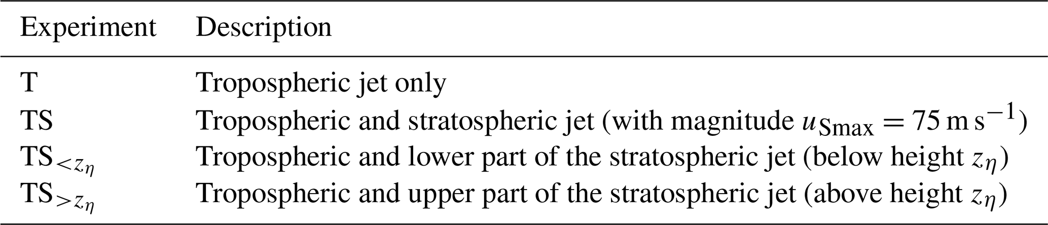
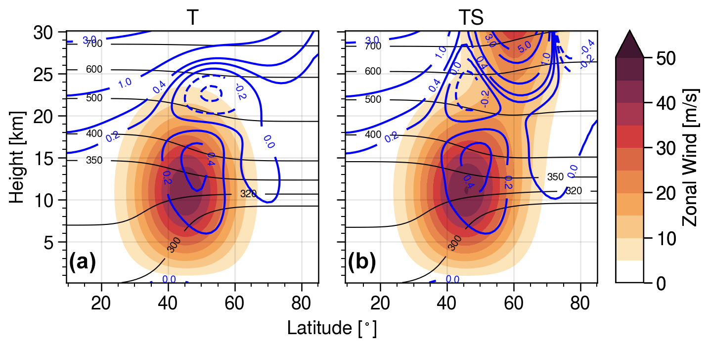
Figure 1 Examples of the basic state used in this study, with different choices for parameter values to include either (a) a tropospheric jet only (experiment T) or (b) a tropospheric and a stratospheric jet (experiment TS). The shading shows the zonal wind, thin black contours show potential temperature (K) and thick blue contours show the meridional PV gradient (PVU per degree), with dashed contours corresponding to negative values.

The temperature distribution of the respective initial state is calculated to be in the thermal wind balance with the prescribed wind field. Note that the resulting meridional PV gradient (thick blue contours in Fig. 1) strongly depends on the vertical curvature of the underlying wind field and, therefore, produces a pronounced local maximum near the tropospheric jet core.

Furthermore, note that both configurations displayed in Fig. 1, due to the strong dependency on the wind field structure, include regions with (a slightly) negative PV gradient, which could potentially influence the evolution of the life cycle. However, the corresponding initial states follow the typical set-up used in this type of idealised life cycle experiment. We further performed a series of sensitivity experiments and concluded that the regions of negative PV gradient have no significant influence on the qualitative results presented in this paper. Magnusdottir and Haynes (1996) also raised the question of the effect of negative PV gradients in typical life cycle set-ups on the evolution of the baroclinic wave and concluded that these regions can have an effect on certain details of the non-linear phase (e.g. details of the energetics) but seem to have no impact on most aspects of the qualitative behaviour.

To trigger the growth of a baroclinic wave, the initial state is perturbed by superimposing a zonally periodic near-surface temperature perturbation of fixed zonal wave number 6, centred around 45^∘ latitude. We found our results to be qualitatively similar for perturbations with wave number 7, but the stratospheric jet has almost no influence on the life cycle for wave numbers 5 and 8 (in these cases, the purely tropospheric life cycle is generally weaker than for perturbations with wave numbers 6 and 7). Our main focus is to study the behaviour of tropospheric waves at synoptic scales, which are primarily forced as a result of baroclinic instability. We expect the mechanisms discussed in the present study to be relevant for synoptic eddy feedbacks involved in real atmospheric stratosphere–troposphere coupling, while acknowledging that planetary waves, which are not explicitly considered here, may also play an important role.

More details on how the basic state is constructed are given in the Appendix. Starting from the described initial conditions, the experiments are then either run freely (without any external forcing) or include a linear Rayleigh surface friction, following the friction profile specified by Held and Suarez (1994), with a maximum friction coefficient of k_f=1 d⁻¹ at the surface, gradually reducing to zero at 700 hPa (z≈3 km).

3 Modification of the life cycle by a stratospheric jet

We start our study by investigating in what way the general evolution of an idealised baroclinic life cycle is altered when the initial conditions include a tropospheric and a stratospheric jet, with the latter representing the wintertime polar vortex, compared to when they include a tropospheric jet only, as is usually the case after a SSW, and it is the conventional life cycle set-up. In the rest of this section, we therefore analyse a set of life cycle experiments with varying values of the stratospheric jet strength parameter u_Smax (see Eq. (A2) in the Appendix) and thus the varying strength of the stratospheric jet that is added to the system with tropospheric jet only.

3.1 Modification of the baroclinic wave breaking

The evolution of idealised baroclinic life cycles is often described in terms of the distribution of potential vorticity (PV) on an isentropic surface close to the jet core (or equivalently close to the tropopause). Zonal modulations in PV contours in this region of sharp PV gradient (also seen in Fig. 1) give insights into the growth and decay of the eddy field, while any change in the position of the maximum in zonally averaged PV gradient represents a meridional shift in the jet. The top and middle rows in Fig. 2 show the horizontal PV distribution on the 350 K isentrope on selected days for the two initial state configurations with tropospheric jet only (experiment T) and tropospheric and stratospheric jet (experiment TS).

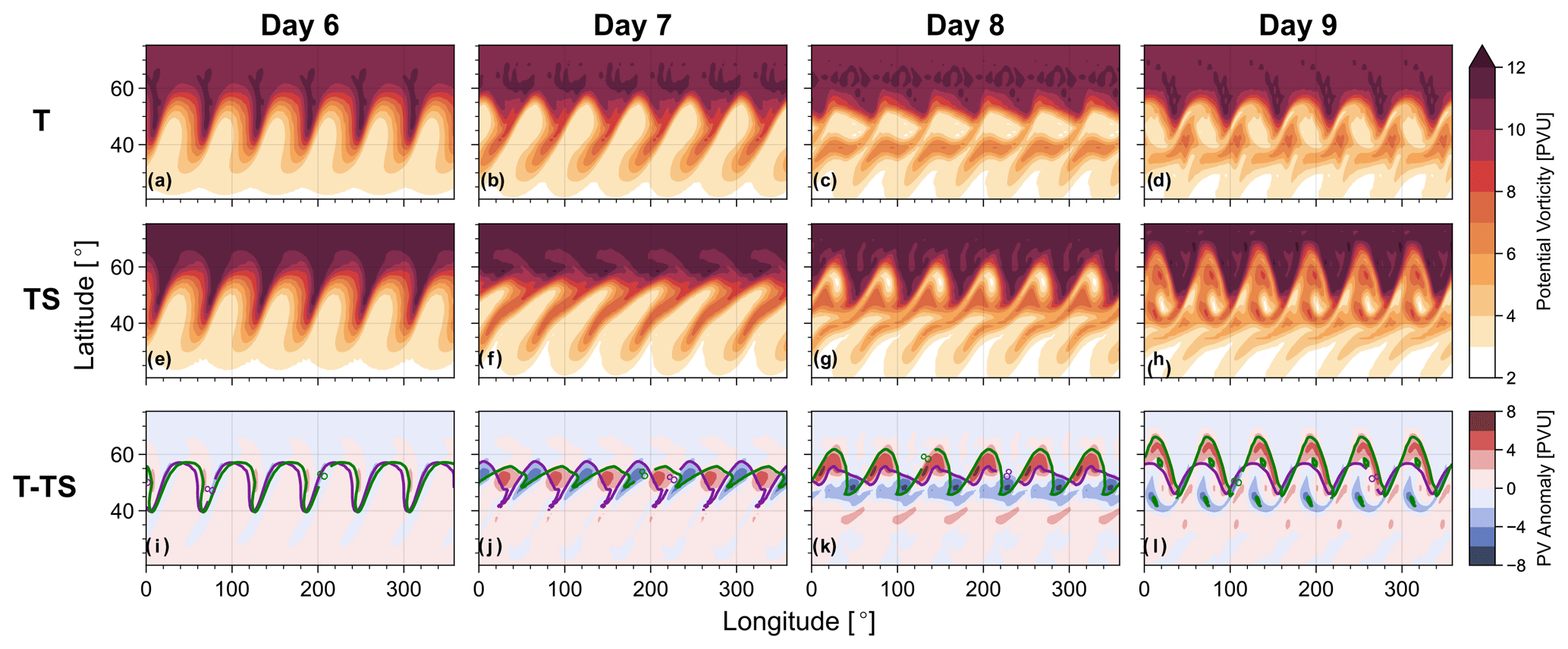
Figure 2 Evolution of PV distribution on the 350 K isentrope on different days for a system with tropospheric jet only (experiment T; a–d) or a tropospheric and stratospheric jet (experiment TS; e–h). Panels (i)–(l) show the difference in both experiments (T–TS), with 8 PVU contours of the respective full fields superimposed.

The general evolution of both experiments is similar to each other in the sense that the baroclinic wave grows gradually until about day 6. At that point, the wave becomes non-linear, breaks and eventually decays. Note that the PV distributions at day 6 are almost identical for the experiments T and TS, suggesting that the difference in evolution during the linear growth phase induced by stratospheric winds is rather small. This represents an important distinction from the previous baroclinic life cycle studies that have highlighted stratospheric impacts during the growth phase (e.g. Wittman et al., 2007; Smy and Scott, 2009). We will discuss this apparent contradiction in more detail later in this section. In contrast to the small differences during the linear phase, the non-linear decay phase shows substantial differences in the specific evolution of the PV field when a stratospheric jet is present. The wave breaking is still characterised by filaments of high PV that stretch out on the equatorward side of the jet core, break off and eventually roll up anticyclonically, but the timing of events and the details of the small-scale structures are altered considerably compared to the tropospheric jet only case. The decay of the baroclinic wave happens faster, and at day 9, a new wave structure seems to have grown already, showing strong characteristics of cyclonic wave breaking (sometimes referred to as the LC2 life cycle in contrast to the anticyclonic LC1 life cycle; see, for example, Thorncroft et al. (1993) for further details).

To highlight the modification in PV evolution induced by the presence of a stratospheric jet, Fig. 2i–l show the difference in the PV field of a simulation with and without stratospheric jet. Overlaid are the corresponding 8 PVU contours of the two respective experiments. It can be seen that at day 6, i.e. at the end of the linear growth phase, the two baroclinic waves have a similar magnitude and structure but are slightly phase shifted with respect to each other. This shift can potentially be explained by a minor increase in phase speed in the case of a stratospheric jet. This might be due to a minor increase in wind speed near the tropopause (also further discussed in Sects. 4 and 5) and/or a change in the corresponding PV gradient in that region due to the slightly modified wind structure in the case of the stratospheric jet. While a pure zonal phase shift in the wave should not have any influence on the subsequent behaviour of the wave breaking due to the zonal symmetry of the system, it does indicate a change in the dispersion relation.

At days 7 to 9, i.e. during the non-linear phase, the evolution of the system is strongly influenced by the stratospheric jet, and Fig. 2 shows a large difference in PV distribution. Especially at days 8 and 9, the baroclinic wave in experiment TS, including a stratospheric jet, seems to have entered a second growth phase, while the wave in experiment T still seems to be decaying. As mentioned in Sect. 1 these secondary life cycles during the non-linear decay phase have been discussed previously by Barnes and Young (1992). We find the details of the non-linear phase, like the occurrence, timing or apparent flavour (in a LC1/LC2 sense) of secondary cycles, to be very sensitive to small changes in the initial conditions or the details of the physical processes involved, as can also be seen in Fig. 2. Recall that, as mentioned in Sect. 2, the occurrence and strength of these secondary cycles varied in a set of sensitivity experiments with lower vertical resolution. For the purpose of this study, we therefore focus primarily on the evolution of the entire life cycle, e.g. in terms of the difference between the initial and some final state.

3.2 Dependency on stratospheric jet magnitude

In addition to the evolution of the PV field, baroclinic life cycles can be quantified in terms of the global energetics of the system, typically with a strong focus on eddy kinetic energy (EKE), which describes the growth and decay of the baroclinic wave in the region of a large meridional PV gradient near the jet core (see Fig. 1). In particular, the decay of EKE is associated with an energy transfer to the zonal mean state, i.e. an increase in the mean kinetic energy (MKE). This increase in MKE can be associated with a poleward shift, and a corresponding acceleration, of the tropospheric jet due to wave–mean-flow interactions and poleward eddy momentum fluxes during the decay phase of the life cycle.

The way the evolution of the life cycle is altered by a stratospheric jet can be seen in terms of EKE and MKE time series, shown in Fig. 3, for experiments with different values for the stratospheric jet magnitude u_Smax (see the Appendix for details). Note that here we use ΔMKE, which is simply the change in MKE with respect to the initial conditions and that both EKE and ΔMKE are displayed as vertically integrated (over the entire atmosphere) and horizontally averaged (over the Northern Hemisphere) energy densities.

In agreement with Fig. 2, which suggests only a phase shift in the baroclinic waves during the linear phase but no difference in magnitudes, Fig. 3 shows essentially no sensitivity to introducing a stratospheric jet before day 6. In particular, we do not find any significant change in growth rate as has been reported by other authors (e.g. Wittman et al., 2007). A potential explanation for the strong change in growth rate found by Wittman et al. (2007) could be a substantial difference in meridional PV gradient (due to the substantial modification of the vertical curvature of zonal wind at the tropopause) between their different experimental set-ups. The basic states used in the present study, on the other hand, only slightly differ in terms of their tropopause level PV gradients (see Fig. 1). However, during the non-linear phase, so from day 7 onwards, the stratospheric jet seems to extensively alter the evolution of the life cycle. This is especially so because the onset of a secondary phase of wave growth (with EKE peaking again at about day 10) seems to happen about a day earlier, when a stratospheric jet is present in the system, and leads to a much stronger and more persistent secondary peak. The persistently elevated EKE of the secondary cycles during the non-linear phase (with EKE reducing again towards the final state) is consistent with the idea of a stronger LC2 flavour (which is often characterised by persistently increased EKE in the decay phase) in the secondary cycles, as also suggested by Fig. 2 and further discussed in Sect. 5.

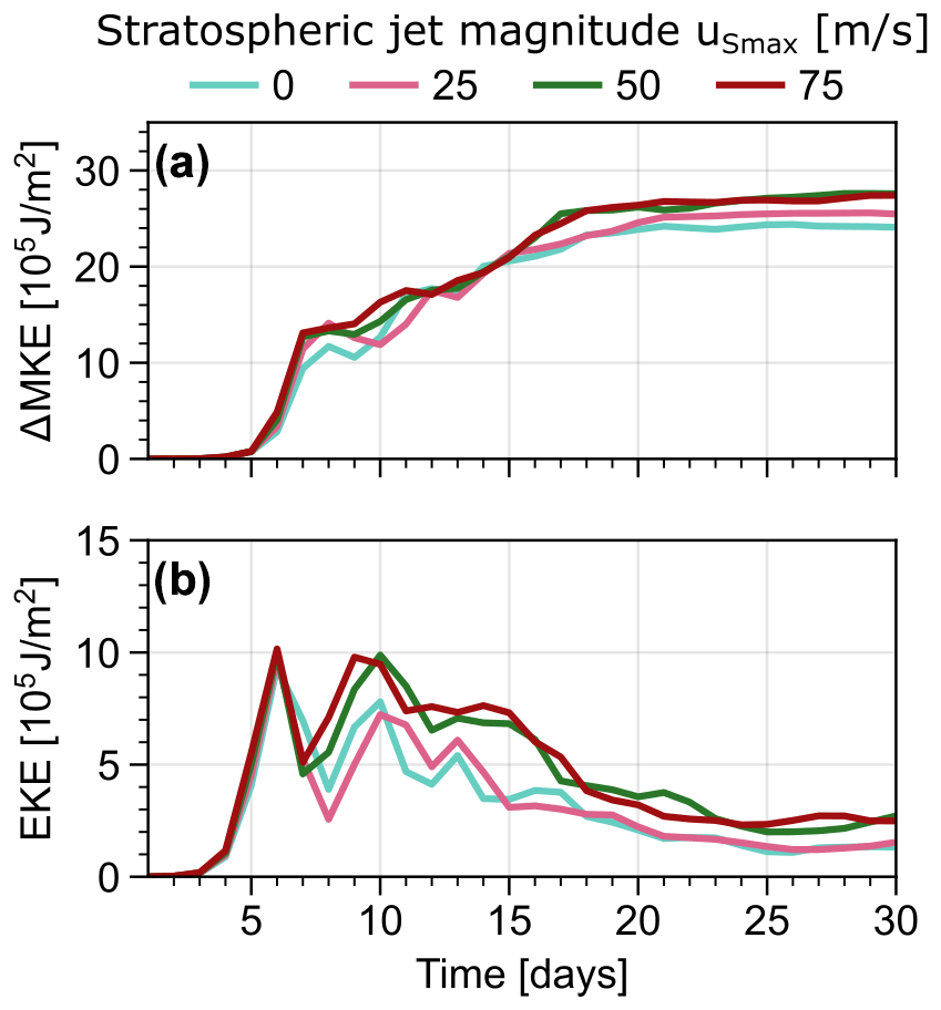
Figure 3 Evolution of mean kinetic energy change (a) and eddy kinetic energy (b) of the system with a tropospheric jet and a stratospheric jet, with varying strength parameter u_Smax (see Eq. A2). The case with u_Smax=0 corresponds to experiment T and the case u_Smax=75 m s⁻¹ to experiment TS. Energies are displayed as vertically integrated and horizontally averaged energy densities.

The alteration of the system as we increase u_Smax not only manifests as changes in the details of how the wave breaking evolves but also leads to a change in the final state (here defined as the average over days 20–30), in particular a systematic increase in ΔMKE.

The elevated values of EKE during the decay phase and ΔMKE in the final state are consistent with an enhanced barotropic conversion of energy from EKE to MKE (see Fig. S2), as also further discussed in Sect. 5. The increase in final state ΔMKE can further be linked to a stronger poleward shift (and correspondingly a stronger acceleration) in the tropospheric jet over the course of the life cycle when a stratospheric jet is present.

This relative shift (compared to the experiment T, with tropospheric jet only) can be seen in Fig. 4, which shows, in all panels, black contours indicating the evolution of the zonal mean zonal wind field at 10 km. Figure 4a furthermore shows the zonal wind anomaly of experiment T with respect to the initial conditions. One can clearly see a dipole pattern developing around the initial jet core (45^∘ latitude) at the start of the non-linear phase at about day 6 and strengthening roughly until day 15, corresponding to a poleward shift in the jet core to about 60^∘ latitude during the life cycle.

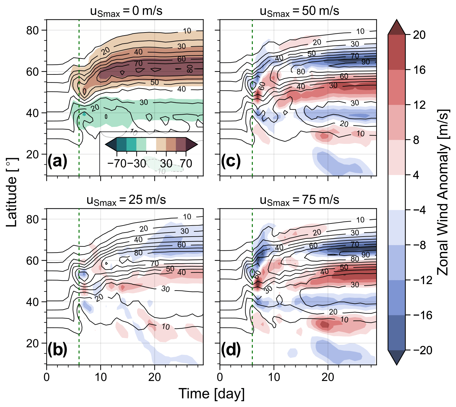
Figure 4 Black contours show the evolution of zonal mean zonal wind (m s⁻¹) on the 10 km surface for experiments with tropospheric jet only (a) or tropospheric and stratospheric jet of varying strength (b–d); the case with u_Smax=0 corresponds to experiment T and the case u_Smax=75 m s⁻¹ to experiment TS. The shading in panel (a) shows the wind anomaly with respect to the initial state. The shading in panels (b–d) shows the wind anomaly induced when the stratospheric jet is removed from the system – i.e. the wind anomalies in panels (b–d) are formed by subtracting the respective wind fields from the wind field shown in panel (a). The vertical dashed lines indicate day 6.

Figure 4b–d show the evolution of the zonal mean zonal wind anomaly at 10 km of experiment TS, with varying strength of the imposed stratospheric jet, relative to experiment T, with tropospheric jet only (i.e. the difference between the wind field of experiment T and the wind field of the respective experiment). The displayed anomaly therefore indicates the changes in zonal mean zonal wind induced by a removal of the stratospheric jet from a system (hence, modelling changes induced by a SSW). As suggested by the MKE time series shown earlier, the zonal wind anomaly evolution indicates a dipole around the position of the final jet core emerging during the non-linear phase of the life cycle. The change in zonal wind corresponds to a stronger poleward shift in the jet during the final state in cases where a stratospheric jet is present or, equivalently, a relative equatorward shift in the tropospheric jet when the stratospheric jet is removed. This jet shift is analogous to the NAM-like signature that has been observed after SSW events, and its appearance in response to stratospheric conditions in the framework of a dry dynamical model further indicates the fundamental importance of tropospheric synoptic-scale eddy feedback in causing the observed negative NAM signal, as has previously been shown by other studies (e.g. Domeisen et al., 2013; Hitchcock and Simpson, 2014), and allows for a way of quantifying these eddy feedback processes (e.g. in terms of EKE and MKE evolution) in a simple and idealised setting.

3.3 Vertical structure of the response and influence of surface friction

The vertical structure of the relative jet shift in the final state can be seen in Fig. 5, showing the difference in zonal mean zonal wind during the final state (days 20–30 mean) between experiments T (with tropospheric jet only) and TS (also including a stratospheric jet of magnitude u_Smax=75 m s⁻¹). Figure 5a shows the latitude height equivalent of Fig. 4d averaged over the final state, while Fig. 5b illustrates the corresponding zonal wind anomaly for an experiment with surface friction applied to the system (see Sect. 2 for details). Both panels show a clear equatorward jet shift signature around the jet core of the final jet when the stratospheric jet is removed. Note that the inclusion of surface friction will lead to a continuous dissipation of energy and, thus, a steady final state is not reached (see the Supplement). However, we define the final state as being analogous to the case without friction (days 20–30 average) in order to analyse the effect of surface friction on the evolution of the main life cycle.

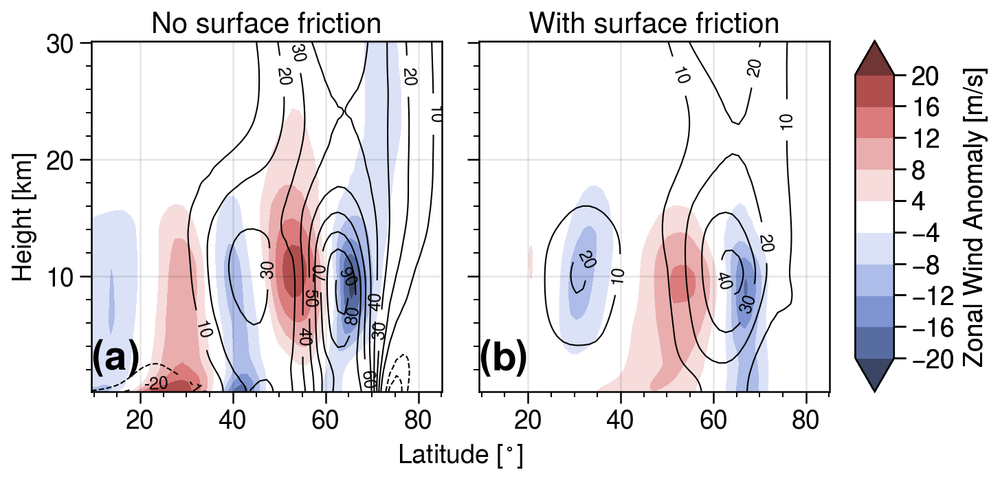
Figure 5 Contours show the zonal mean zonal wind (m s⁻¹) of the final state (days 20–30 average) of a system with a stratospheric jet. Shading indicates changes to the final state zonal mean zonal wind when the stratospheric jet is removed from the system. Panel (a) shows an experiment without surface friction, while panel (b) displays an experiment with surface friction as described in Sect. 2.

Several differences can be observed in the final state of the life cycle for systems with and without surface friction. First, an overall weakening of the jet in the final state (black contours) can be observed when surface friction is included, which is easily explained by the direct dissipation of kinetic energy over the course of the life cycle due to the added friction process. The same argument holds for the disappearance of the strong wind anomaly patterns close to the surface at about 30 and 40^∘ latitude in the case without friction. These patterns develop due to strong temperature fluxes in this region arising from the large meridional surface temperature gradient (see Fig. 1), and they are likely not influential on the standard baroclinic life cycle evolution. More importantly, however, the vertical structure of the dipole pattern around the final jet core at 60^∘ latitude is drastically different between the experiments with and without surface friction displayed in Fig. 5. When the system is subject to surface friction during the life cycle, the corresponding dipole pattern is more barotropic; thus, it extends much further down and shows much stronger anomalies at the surface.

Figures 4 and 5 indicate a tendency of the tropospheric jet to exhibit a weaker poleward shift during the baroclinic life cycle if there is no stratospheric jet present compared to when there is. This behaviour is consistent with the negative NAM response, associated with an equatorward shift in the tropospheric jet, observed during periods following SSWs (see Baldwin and Dunkerton, 2001). It further provides a simple model framework to quantify the eddy feedback processes (e.g. in terms of EKE and MKE response) potentially involved in creating the corresponding jet shift signal. Figure 5 shows the shift signal to only have a significant surface contribution if the system is subject to surface friction.

To further illustrate the surface signal observed in our model experiments, Fig. 6 shows the geostrophic geopotential height field Z, calculated by solving the following equation:

$$\begin{array}{}\text{(2)}& {\partial }_{\mathit{\varphi }}Z=-fa\stackrel{\mathrm{‾}}{u}-{\stackrel{\mathrm{‾}}{u}}^{\mathrm{2}}\tan \mathit{\varphi },\end{array}$$

via simple numerical integration with boundary condition $Z(\mathit{\varphi }=\mathrm{0})=\mathrm{0}$ for the zonal mean zonal wind field $\stackrel{\mathrm{‾}}{u}$ of the final state (note that we neglected the surface friction term in Eq. (2) as it tends to be small during the final state of our experiments). Here, f is the Coriolis parameter, a the radius of the Earth, g the gravitational acceleration and ϕ the latitude. Since $\stackrel{\mathrm{‾}}{u}(z=\mathrm{0})$ vanishes for the initial state, the surface geopotential height $Z_{\mathrm{sfc}}\equiv Z(z=\mathrm{0})$ of the final state (or more precisely its gradient) describes the change in surface winds induced over the course of the baroclinic life cycle.

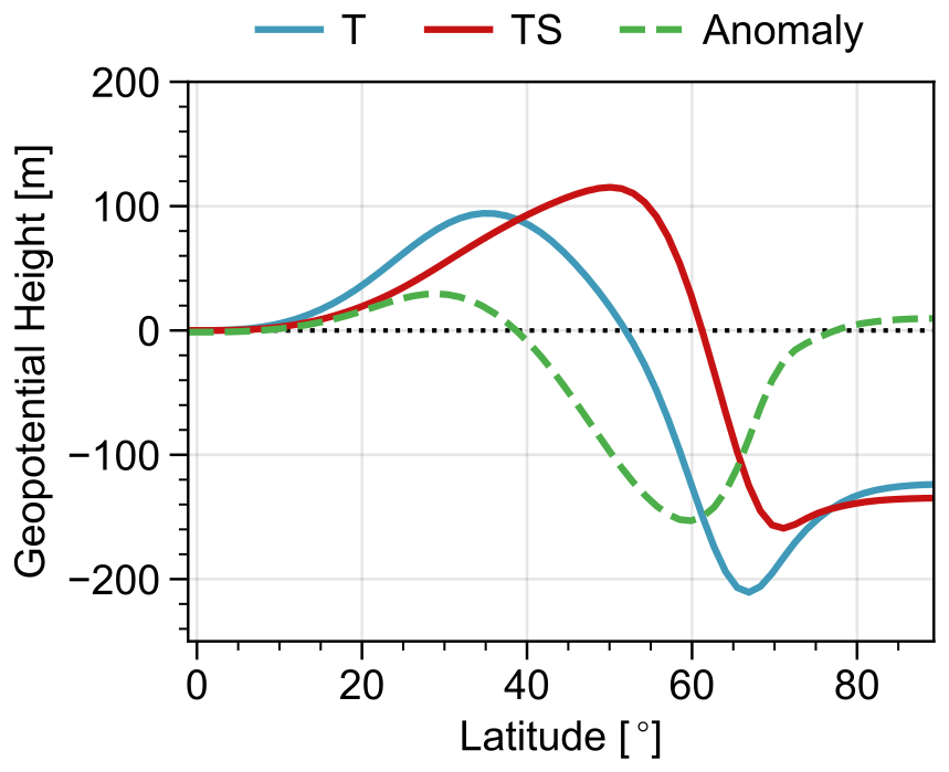
Figure 6 Zonal mean geopotential height at 1000 hPa (or, equivalently, z=0) of the final state for two experiments with surface friction and with tropospheric jet only (T) and tropospheric and stratospheric jet (TS), respectively. The dashed line shows the difference in both.

Figure 6 shows Z_sfc for experiments that include surface friction and two different sets of initial conditions, i.e. T and TS, which, respectively, include a tropospheric jet only and include both a tropospheric and a stratospheric jet. For both experiments, we find the development of strong meridional gradients in Z_sfc at around 50 or 60^∘ latitude, respectively, consistent with strong surface winds. The further equatorward shifted position of the gradient of Z_sfc in experiment T, relative to experiment TS, indicates again the relative equatorward shift in the final tropospheric jet if the stratospheric jet is removed from the initial conditions, corresponding to the NAM signal discussed earlier.

The strength of the NAM-like jet shift signal depends on the magnitude of the stratospheric jet (u_Smax) included in the system, as can be seen in Fig. 7. First, the NAM signal, in the form of a dipole jet shift pattern around 60^∘ latitude, seems to develop for stratospheric jet magnitudes below about u_Smax⪅50 m s⁻¹ but stays mostly unchanged for stratospheric jets exceeding u_Smax⪆50 m s⁻¹. Second, the NAM response does not seem to be symmetric for positive and negative values of u_Smax. While the jet shift signal develops for relatively weak westerly stratospheric jets, no coherent signal can be observed for easterly stratospheric jets for the parameter range shown (a positive NAM signal, i.e. a relative poleward shift, only starts to develop for u_Smax⪅−40 m s⁻¹).

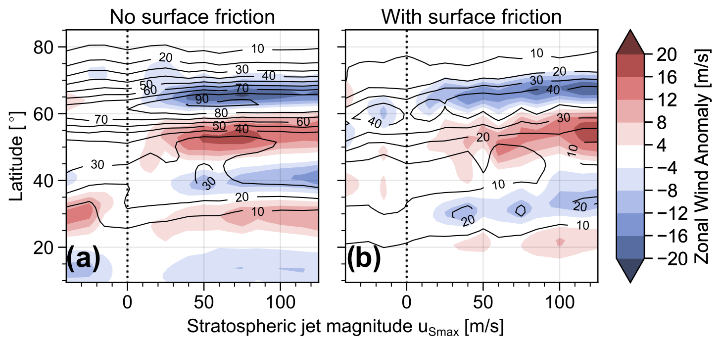
Figure 7 Contours show the zonal mean zonal wind at 10 km of the final state of experiments that include a stratospheric jet with the varying strength parameter u_Smax. Shading represents the changes induced when the stratospheric jet is removed from the system. Panels (a) and (b) show the experiment without and with surface friction, respectively. The vertical dotted line indicates u_Smax=0 and, thus, experiment T.

In the rest of this paper, we investigate the influence of a stratospheric jet on the final state of the baroclinic life cycle, and the resulting NAM-like signature, in more detail. In particular, we identify a region in the lower stratosphere which is highly sensitive to changes in the zonal wind that are induced by the inclusion of a stratospheric jet.

4 Sensitivity of the life cycle to changes in the extratropical lower stratosphere

In the previous section, we established that introducing a stratospheric jet can modify the evolution of the system in an idealised baroclinic life experiment, as has also been shown by other authors (e.g. Wittman et al., 2004). In this section, we show that the system is particularly sensitive to changes in wind structure in the extratropical lower stratosphere (heights below about 25 km), while changes in the middle and upper stratosphere have almost no influence on the final state. In order to investigate this sensitivity, we analyse a set of experiments with initial conditions that include a tropospheric jet and a stratospheric jet with a modified vertical structure.

We modify the structure by multiplying the profile of the stratospheric jet used in experiment TS by a function η(z) (see Eq. A2). We choose η(z) to follow a Tanh profile, which allows us to smoothly set the winds of the stratospheric jet component to zero, either below or above a set transition height z_η, and thus investigate which part of the stratospheric jet has the strongest influence on the life cycle. We hereby refer to the experiments in which we only include the part of the stratospheric jet below height z_η as “${\mathrm{TS}}_{<z_{\mathit{\eta }}}$”, and correspondingly refer to the experiments in which we keep the part above z_η as ${\mathrm{TS}}_{>z_{\mathit{\eta }}}$ (for simplicity, we drop the units of z_η within this notation and set it to be kilometres). See the Appendix for details on how the basic state is defined.

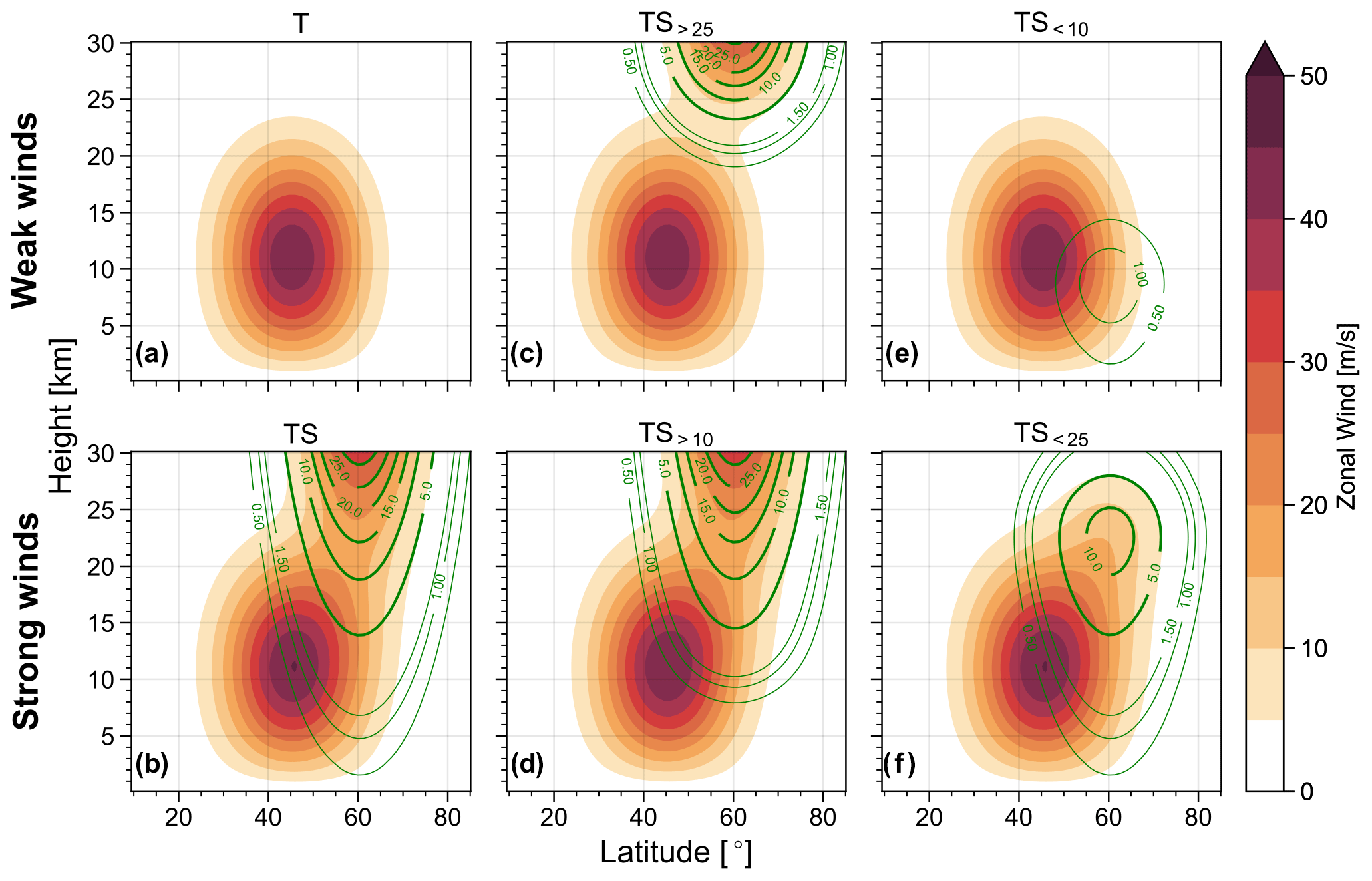
Figure 8 Zonal wind (shading) and anomaly from experiment T (green contours in m s⁻¹) of the initial conditions for experiments with a tropospheric jet and varying vertical profiles of the superimposed stratospheric jet, depending on the function η(z) in Eq. (A2). Note that both sets of green contours, thick and thin, show the same quantity but for different level ranges.

Figure 8 illustrates the different basic states in terms of the full zonal mean zonal wind field and the anomaly with respect to experiment T, i.e. the experiment without any superimposed stratospheric jet. Figure 8a and b show experiments T and TS, including either no or the full stratospheric jet, respectively. The experiments displayed in Fig. 8b and c only superimpose the upper part of the stratospheric jet, above either 25 or 10 km, while the experiments displayed in Fig. 8e and f only include the respective lower parts.

Details of the vertical structure of the various initial wind fields can also be seen in Fig. 9, displaying the zonal wind at 60^∘ latitude, i.e. at the northern flank of the tropospheric jet and through the core of the stratospheric jet. A very prominent difference is that profiles in which the stratospheric jet reaches into the lower stratosphere have substantially increased wind speeds in that region (roughly between 10 and 25 km), compared to profiles in which the contribution of the jet is mostly confined to the troposphere or the middle and upper stratosphere. This criterion divides the six profiles into two groups, with one consisting of profiles T, TS_>25 and TS_<10 with weak winds in the lower stratosphere, and the other consisting of profiles TS, TS_>10 and TS_<25 with strong winds in the lower stratosphere. In most of the rest of this section, we analyse the experiments with different initial conditions, keeping in mind the grouping into these two sets.

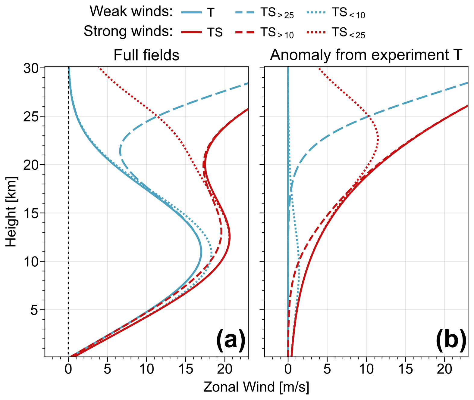
Figure 9 Vertical profiles of zonal mean zonal wind at 60^∘ latitude of the initial conditions for different experiments without (T), with full (TS) or with partial stratospheric jet (other profiles). Panel (a) shows the full fields, and panel (b) shows the anomaly from experiment T.

To visualise the NAM-like jet shift signature of the final state, and to investigate which contribution to this jet shift can be associated the different parts of the stratospheric jet, Fig. 10 shows the zonal mean zonal wind averaged over days 20–30 and the corresponding anomaly from experiment T (with tropospheric jet only).

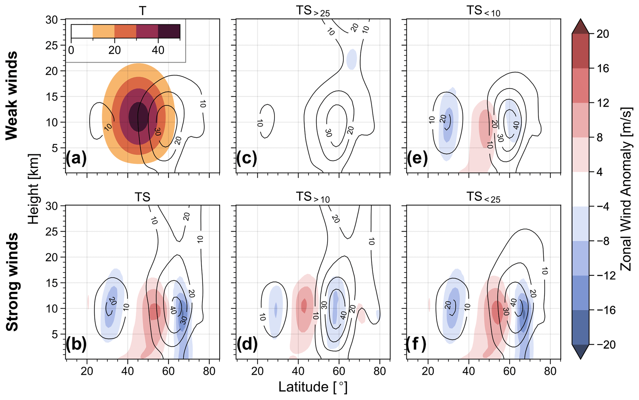
Figure 10 Black contours show the zonal mean zonal wind (m s⁻¹) distribution of the final state for different experiments. The shading in panel (a) indicates the initial zonal winds (m s⁻¹) of experiment T, and the shading in panels (b–f) shows the anomaly from experiment T in zonal mean zonal wind of the final state. All experiments include surface friction.

We first look at the experiments with weak winds in the lower stratosphere. The final state zonal wind field of experiment TS_>25 (Fig. 10c) does not show any substantial deviation from experiment T, indicating that winds in the middle and upper stratosphere have virtually no influence on the life cycle. Experiment TS_<10, with superimposed winds confined to the troposphere, shows a dipole pattern, which could potentially be attributed to the projection of the wind modification on, for example, the increase in tropospheric jet magnitude or the vertical shear, which is also further discussed in Sect. 5. However, also note that the superimposed winds of the stratospheric jet do not abruptly vanish at the given cut-off height (e.g. above 10 km for TS_<10) but follow a smooth transition over the course of about 4 km and, therefore, still reach into the lower stratosphere region.

The experiments with strong winds in the lower stratosphere (bottom row of Fig. 10) all show a clear dipole structure in the anomaly field, centred at about 60^∘ latitude. Note, in particular, the strong signal of experiment TS_<25, where the superimposed winds are confined to the troposphere and lower stratosphere, further suggesting that the winds in the middle and upper troposphere have no significant contribution to causing the observed jet shift. Experiment TS_>10, including a stratospheric jet that reaches into the lower stratosphere but does not reach far into the troposphere, also shows a clear dipole pattern in zonal wind anomaly. In particular, compare experiments TS_>10 and TS_>25 as well as TS_<25 and TS_<10. In both cases, the jet shift signal increases in strength when the superimposed stratospheric jet reaches into the lower stratosphere (10 to 25 km) compared to when it does not. The significance of the lower stratospheric wind anomalies is discussed further in Sect. 5.

The surface signal of the NAM-like response discussed above can be seen in Fig. 11, which displays the zonally averaged geopotential height field calculated via Eq. (2). It can clearly be seen how the different experiments show indications for NAM-like surface signals, which is in good agreement with what is shown in Fig. 10. In particular, the experiments with strong lower stratospheric winds (bottom row) show a poleward shift and acceleration in the surface winds (in terms of the gradient of the shown curves) relative to the reference experiment T, with only the tropospheric jet.

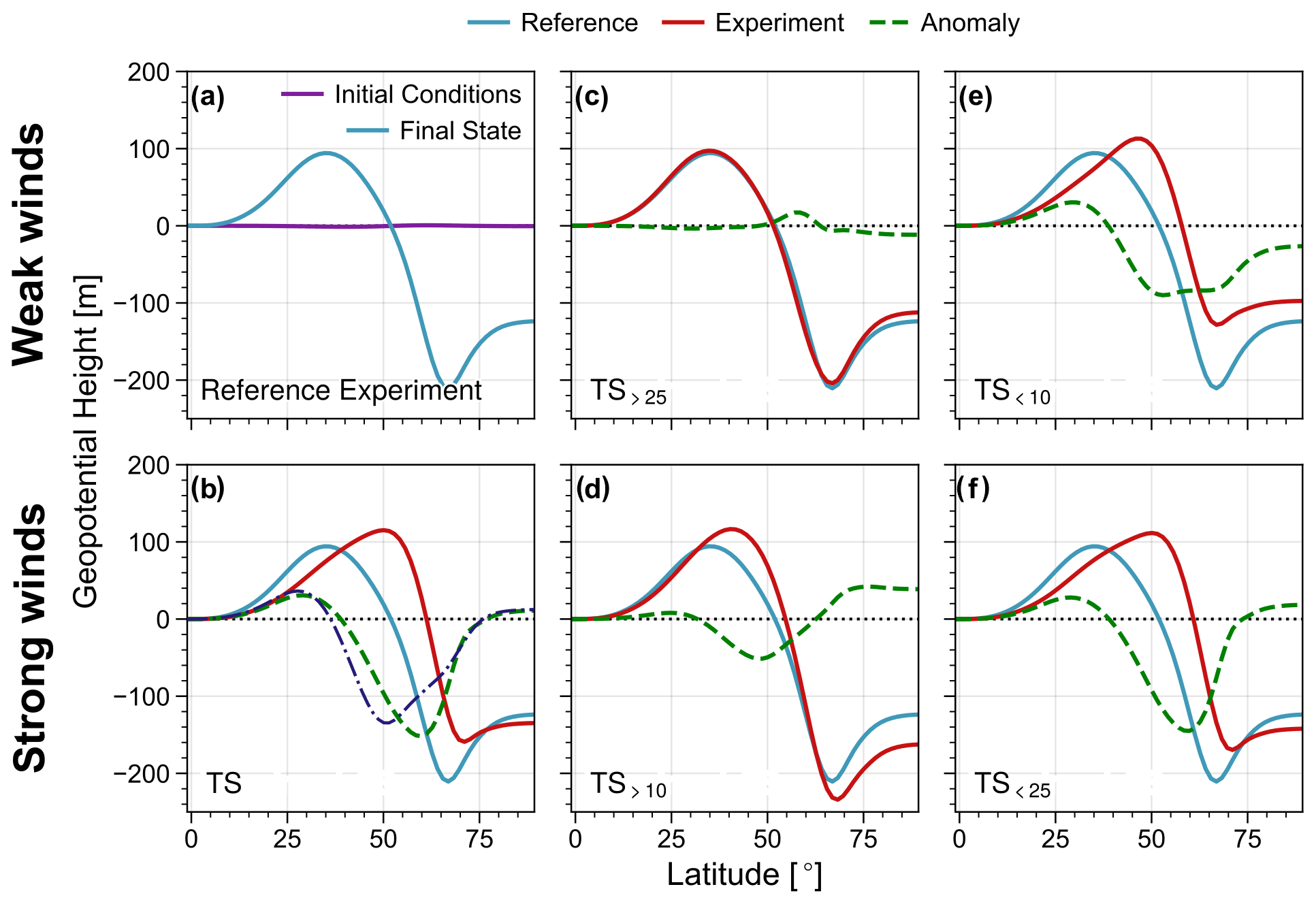
Figure 11 Geopotential height at 1000 hPa of the final state of the experiments displayed in Fig. 8. Panel (a) illustrates the difference in the initial and final state geopotential height for experiment T; all other panels illustrate the difference between the respective experiment and the reference experiment T. The purple dashed–dotted line in panel (b) shows the sum of the anomalies for the cases T_<10 and T_>10. All experiments include surface friction.

Figure 11b further shows the sum of the geopotential height anomalies induced by removal of the (partial) stratospheric jet from the experiments T_<10 and T_>10, i.e, experiments where we only include the part of the stratospheric jet above or below 10 km. The similarity of this sum to the corresponding geopotential height anomaly of experiment TS, with full stratospheric jet included, suggests a certain additivity of the response to the stratospheric jet¹, which is also further discussed in Sect. 5.

5 Discussion

In Sect. 3 we showed that the growth phase of an idealised baroclinic life cycle is almost unchanged when introducing a stratospheric jet to the system. In particular, the linear growth rate of the baroclinic wave (in terms of EKE) is not sensitive to changes in stratospheric conditions. These findings seem to contradict previously reported results (e.g. Wittman et al., 2007; Smy and Scott, 2009). A likely explanation for this discrepancy is that the linear growth phase is highly sensitive to tropopause level PV gradients of the initial conditions, which had been altered due to changes in the stratosphere in these previous studies. The structure of the PV gradient in our experiments, on the other hand, is essentially not altered by the inclusion of stratospheric winds, and the linear growth of baroclinic waves (driven by tropospheric heat fluxes) is therefore unchanged. However, we found that the presence of a stratospheric jet substantially altered the non-linear decay phase of the life cycle. Notably, it is during this decay phase when the eddy momentum flux acts to convert the eddy kinetic to mean kinetic energy while, at the same time, driving a meridional shift in the tropospheric jet. Given that the momentum flux is proportional to the equatorward wave activity flux, our findings are consistent with a stratospheric influence via modifications to meridional wave propagation near the tropopause.

Figures 2 and 3 show changes in the secondary cycles occurring during the non-linear decay stage, including changes in number, strength, duration, timing and the apparent type (or flavour) of these secondary cycles. The different types of baroclinic wave breaking (LC1 and LC2) have been linked to different weather regimes, and thus, corresponding transitions within a life cycle can potentially have a large impact on surface weather (e.g. Michel and Rivière, 2011). As discussed, the baroclinic decay phase of experiment TS shows characteristics of both the LC1 and LC2 flavour or, equivalently, cyclonic and anticyclonic wave breaking, while experiment T shows more LC1 characteristics. However, the general behaviour of the TS life cycle (e.g. in terms of its final state) still primarily follows the (anticyclonic) LC1 type, and it only seems to experience individual, transient (cyclonic) LC2 wave breaking events. The importance of these transient LC2 events for the overall meteorological regime is presently not clear. Note that other authors have previously also reported on transitions between LC1 and LC2 wave breaking states based on stratospheric conditions (e.g. Kunz et al., 2009), but mostly in terms of the entire life cycle, rather than in terms of more transient events.

Further note that the introduction of a stratospheric jet not only modifies the details of the wave breaking during the decay phase, but also the (quasi-steady) final state of the life cycle. In particular, generally elevated values of EKE during the decay phase and increased MKE during the final state suggest an enhanced barotropic EKE to MKE conversion (as also seen in Fig. S2). The inclusion of a stratospheric jet to a basic state also formally corresponds to an increase in MPE (mean potential energy, also referred to as available potential energy or APE), where the latter, in principle, forms the main energy source for the life cycle and is, via EKE, ultimately converted into MKE. However, since this increase in MPE is primarily associated with stratospheric temperature structure, it is unlikely to contribute to the predominantly tropospheric energy conversions during the life cycle.

Consistent with the change in final state MKE, we observed a relative equatorward shift in the tropospheric jet in the final state when removing the stratospheric jet from the initial conditions of the system, as can be seen in Figs. 5 and 6. This relative jet shift is analogous to the NAM-like signature that has been observed after SSW events. To what extent the observed NAM response to SSWs is similarly influenced by tropospheric eddy feedbacks, as suggested by our results, remains to be quantified further. It also is important to remember that the coupling of troposphere and stratosphere works in both directions, and the coupled system will generally react as a whole to any (tropospheric or stratospheric) forcing.

We further want to point out that the relative meridional shift between the final jet in the experiments T and TS results from differences in the meridional eddy momentum transport during the life cycle (not shown). The increased momentum fluxes in experiment TS, compared to T, can be related to increased wave activity around tropopause level, which is consistent with the increase in EKE shown in Fig. 3. Similar changes in eddy momentum transport as a result of (in particular lower stratospheric) climate anomalies have been observed previously in idealised general circulation model experiments by various authors (e.g. Polvani and Kushner, 2002; Butler et al., 2010).

Figure 5 further shows that the surface signal of the NAM response in the final state, given by the zonal mean zonal wind difference between experiments T and TS, is enhanced when the system is subject to surface friction. The effect of surface friction on increasing the surface wind signal of the NAM response might seem counter-intuitive. However, as we already pointed out in Sect. 1.3, surface friction can provide a way for tropopause level eddy momentum fluxes to couple to the surface winds. The modification of the baroclinic eddy field by the presence of a stratospheric jet can therefore project more strongly onto the surface winds and produce a stronger surface signal. The evolution equation of the vertically averaged zonal mean zonal wind (Eq. 1) is often used to argue that, on long timescales (where ${\partial }_t\left[\stackrel{\mathrm{‾}}{u}\right]\approx \mathrm{0}$), the eddy flux convergence has to be balanced by the (dissipation of) surface winds. In our (transient) life cycle experiments, we cannot neglect the wind tendency term, and the main balance is given by ${\partial }_t\left[\stackrel{\mathrm{‾}}{u}\right]\approx -{\partial }_y\left[\stackrel{\mathrm{‾}}{u^{\prime }{v}^{\prime }}\right]$. However, the dissipation term ${\stackrel{\mathrm{‾}}{u}}_{\mathrm{sfc}}/\mathit{\tau }$ provides an important contribution to the equation and strongly modifies the acceleration of the jet, as is already suggested by the factor 2 difference of the final jet magnitude in the cases with and without surface friction (see Fig. 5).

When interpreting Eq. (1), one also has to keep in mind that it describes the evolution of the full (vertically and zonally averaged) wind field, whereas we are mostly interested in the enhanced surface signal of the difference in wind field between experiments TS and T (see Fig. 5), i.e. the NAM-like shift signal. The line of argument, however, is analogous. The introduction (or removal) of a stratospheric jet influences the evolution of baroclinic eddies at tropopause level. Following Eq. 1, the corresponding changes in eddy momentum flux then induce changes in the wind tendency (which will tend to be close to the level of the eddy flux, primarily near the tropopause) but also couple directly to the surface winds.

The enhancement of the surface signal by surface friction can potentially be understood via the following mechanism: the decay stage of the life cycle is characterised by a barotropisation of the tropospheric jet and, thus, a reduction in vertical shear and a strengthening of surface winds. The surface friction, on the other hand, tends to increase the vertical wind shear and, therefore, act as a source of baroclinicity. This increase in baroclinicity then leads to an enhanced barotropisation of the jet (similar to what was observed by Barnes and Young, 1992) and a correspondingly enhanced downward propagation of the jet shift signal. The idea of an enhanced baroclinisation/barotropisation is consistent with the formation of additional life cycles which we observed during the late stages of the life cycle in experiments with surface friction (seen roughly between days 15 and 25 in Fig. S3).

Figure 7 indicated that the strength of the NAM response following the removal of the stratospheric jet depends non-linearly on the magnitude of the stratospheric jet. In particular, the signal seems to saturate when the stratospheric jet magnitude exceeds a certain value, and stronger jets do not lead to a stronger NAM signal any more. This behaviour suggests that an anomalously strong polar vortex does not necessarily lead to anomalously positive NAM signals. Similarly, Fig. 7 indicates that a reversal of the stratospheric jet (with u_Smax<0) does not lead to a negative NAM response with respect to experiment T, which suggests that, in terms of NAM response, it is not important whether a SSW leads to slightly or strongly reversed winds of the polar vortex. However, the set-up of the baroclinic life cycle experiments does, of course, not capture the dynamics around SSWs in their entire complexity, and these results do not necessarily carry over to the real atmosphere.

In Sect. 4, we showed that the NAM response observed in the final state of our life cycle experiments is mostly caused by the change in wind structure in the lower stratosphere when including the stratospheric jet, rather than wind anomalies, in the middle and upper stratosphere (Fig. 10). The sensitivity of the eddy feedback to wind anomalies in the lower stratosphere is consistent with results previously reported by various authors (e.g. Butler et al., 2010).

It should be noted that changing the wind structure in the lower stratosphere also introduces changes in various other characteristics of the corresponding initial conditions, like the height of maximum wind speed, the vertical wind shear in the upper troposphere (roughly up to 10 km) and the magnitude of the tropospheric jet (especially obvious for profiles T and TS in Fig. 9). However, these three characteristics are intrinsically not completely independent and can all potentially affect the evolution of the life cycle. This can be seen, for example, since the vertical wind shear is (via thermal wind balance) related to the horizontal temperature gradient, which drives the growth of baroclinic waves and can, among other things, modify their (linear) growth rate (although note that the near-surface shear is almost identical in the different experiments).

We performed a set of sensitivity experiments (not shown) with tropospheric jet only and varying tropospheric jet magnitude (and therefore increased vertical shear in the troposphere). We found that an increase in tropospheric jet strength also leads to an increased poleward shift during the life cycle (i.e. an equatorward shift in the jet in the final state of experiment T relative to a case with stronger tropospheric jet), similar to the shift observed in Fig. 5a. In order to achieve a jet shift signal of similar magnitude to the one shown in Fig. 5, however, it was necessary to increase the jet magnitude by an order of 10 m s⁻¹ in these sensitivity experiments (the difference in tropospheric jet magnitude between experiments T and TS is only of the order of 1 m s⁻¹), indicating that other characteristics of the initial state need to contribute, and the observed jet shift cannot purely be a result of a strengthened tropospheric jet. The inclusion of the stratospheric jet does, to some extent, project the mentioned characteristics (e.g. height of the jet core and tropospheric shear) of the total zonal wind profile, and the resulting jet shift can potentially be interpreted as the result of a combination of factors.

Figure 11 further suggests that we essentially recover the surface geopotential height signal of experiment TS (with full stratospheric jet) when adding the corresponding signals of experiments T_<10 and T_>10. Such additivity of the responses might be another indication that the stratospheric jet projects onto various other structures and characteristics (e.g. tropospheric shear and jet core height), and the corresponding jet shift response forms as a result of a combination of responses to those modifications. However, while the anomalies of the respective experiments seem to be additive when it comes to the surface geopotential height (although not perfect), the middle tropospheric jet shift response in Fig. 10 does not appear to follow the same additive behaviour.

As discussed, Fig. 10 shows the NAM-like jet shift signature of the life cycle due to the inclusion of a stratospheric jet to be mainly caused by the corresponding change in winds in the lower stratosphere, rather than the winds in the middle and upper stratosphere, where the stratospheric jet itself is strongest. A similar conclusion can be drawn from the energetics of the system (provided in the Supplement), which shows a consistent increase in the MKE of the final state for the experiments with strong winds in the lower stratosphere (as defined in Sect. 4), compared to the experiments with weak winds in a system that does not include surface friction. As also explained in Sect. 3, this increase in MKE is caused by the relative meridional shift in the final tropospheric jet. Note that if the system includes surface friction, the constant dissipation of wind leads to a gradual and flow-dependent decrease of MKE, which makes the interpretation of the energetics in terms of a final state difficult. However, we find basic states which include a stratospheric jet to be associated with an enhanced barotropic energy conversion of EKE to MKE during the life cycle in both systems that do and do not include surface friction (see Fig. S2).

While the present study discusses the sensitivity of the tropospheric jet shift to the presence of a stratospheric jet during baroclinic life cycles in some detail, various questions remain open and provide the potential for future work. It might be possible to use the idealised life cycle set-up discussed above to gain insights into the distinction between the responses to different types of SSWs. For example, sudden stratospheric warming events, characterised as split or displacement, have been found to be associated with different lower stratospheric wind anomalies, while the question of differences in their tropospheric response has not been fully answered (see Charlton and Polvani, 2007; Mitchell et al., 2011; Maycock and Hitchcock, 2015). Smy and Scott (2009) studied the distinction between split and displacement events in idealised life cycle experiments and found strong differences in the tropospheric response. However, it should be noted that their experiments are initialised with a basic state constructed via the inversion of an imposed PV field, which will inevitably have an influence on the tropospheric initial state and, thus, directly affect the evolution of the life cycle. The distinct stratospheric influences via direct remote PV signatures or indirect influences on non-linear baroclinic eddy dynamics remains to be investigated further.

6 Summary and conclusions

In this paper, we discussed changes in the evolution of idealised baroclinic life cycles induced by the presence of a stratospheric jet. Particular attention was given to a jet shift signal in the zonal wind anomaly of the final state of the life cycle, similar to the signature of negative (surface) anomalies of the northern annular mode (NAM) often observed after sudden stratospheric warming (SSW) events.

We found that the final state of the life cycle is associated with increased zonal mean kinetic energy when a stratospheric jet is included in the system, roughly representing the polar vortex of typical wintertime conditions, compared to the typical life cycle set-up including only a tropospheric jet, roughly representing post-SSW conditions. This increase in mean kinetic energy corresponds to a negative NAM signal in the final state zonal wind, i.e. a relative equatorward shift in the tropospheric jet in the case with the tropospheric jet only compared to the case with tropospheric and stratospheric jet. The negative NAM signal is the result of a reduced poleward shift over the course of the life cycle induced by a reduction in eddy momentum transport at tropopause level.

The corresponding NAM-like jet shift response has an increased surface signal if the system includes surface friction, which might seem counter-intuitive but is consistent with the idea of an increased coupling of surface winds to the eddy momentum transport at the tropopause level due to the friction.

We further showed that the system is mainly sensitive to changes in the wind structure in the lower stratosphere (heights between 10 and 25 km) rather than to zonal wind anomalies in the middle and upper stratosphere.

The findings of this paper provide further evidence of the role of tropospheric eddy feedbacks in shaping the tropospheric response to stratospheric events. In particular, they help to explain the observed negative surface NAM signal following SSWs. The simplified nature of the idealised life cycle set-up allows for a clean separation of tropospheric eddy feedbacks in the surface response to different stratospheric conditions, highlighting the role of tropopause level momentum fluxes in the non-linear phase of the life cycle. It furthermore offers quantitative insights into the role of surface friction in modulating the surface response to stratospheric events in a simplified setting.

Appendix A: Construction of initial state

The basic state used to initialise our experiments is defined via a zonally symmetric zonal wind field consisting of the following two individual components: a tropospheric jet U_T (representing the mid-latitude jet) and a stratospheric jet U_S (representing the polar vortex). The total wind field is then given by the sum of both components $U=U_{\mathrm{T}}+U_{\mathrm{S}}$, with the tropospheric jet profile being given by the following:

$$\begin{array}{}\text{(A1)}& \begin{array}{rl}{U}_{\mathrm{T}}=& u_{\mathrm{Tmax}}\left(z/z_{\mathrm{Tmid}}\right)\exp \left(\left(\mathrm{1}-{\left(z/z_{\mathrm{Tmid}}\right)}^{\mathit{\alpha }}\right)/\mathit{\alpha }\right)\\ & {\sin }^{\mathrm{3}}\left(\mathit{\pi }{\sin }^{\mathrm{2}}\left(\mathit{\varphi }\right)\right),\end{array}\end{array}$$

where $z=-H\ln (p/p_{\mathrm{0}})$ is a log-pressure coordinate with scale height H=7.5 km and reference pressure p₀=1000 hPa, and ϕ describes latitude. The parameters u_Tmax, z_Tmid and α can be used to modify the jet strength, the core height and the depth of the jet, respectively. The corresponding stratospheric jet profile is defined as follows:

$$\begin{array}{}\text{(A2)}& \begin{array}{rl}{U}_{\mathrm{S}}& =u_{\mathrm{Smax}}\mathit{\eta }\left(z\right)\exp \left(-{\left(z-z_{\mathrm{Smid}}\right)}^{\mathrm{2}}/\mathrm{\Delta }{z}_{\mathrm{S}}^{\mathrm{2}}\right.\\ & \left.-{\left(\mathit{\varphi }-{\mathit{\varphi }}_{\mathrm{S}}\right)}^{\mathrm{2}}/\mathrm{\Delta }{\mathit{\varphi }}_{\mathrm{S}}^{\mathrm{2}}\right),\end{array}\end{array}$$

where u_Smax determines the strength of the jet, z_Smid and ϕ_S its core position and Δz_S and Δϕ_S its width and depth, respectively. Note that we restrict both jet profiles to the Northern Hemisphere, i.e. for ϕ<0 we choose $u_{\mathrm{Tmax}}=u_{\mathrm{Smax}}=\mathrm{0}$ and, therefore, keep the Southern Hemisphere of the basic state at rest.

The function η(z) can be used to further modify the vertical structure of the stratospheric jet. For all experiments in Sect. 3 we choose η≡1 so the stratospheric jet is unmodified, while for the cut-off experiment in Sect. 4 we choose the following:

$$\begin{array}{}\text{(A3)}& \mathit{\eta }\left(z\right)=\mathrm{0.5}\left(\mathrm{1}\pm \tanh \left(\left(z-z_{\mathit{\eta }}\right)/\mathrm{\Delta }{z}_{\mathit{\eta }}\right)\right),\end{array}$$

in order to set the stratospheric jet strength to zero above or below (depending on whether a plus or minus is used within Eq. A3) the transition height z_η, with a smooth transition of depth Δz_η. This gives us a way to isolate the parts of the stratospheric jet within the troposphere, lower stratosphere or middle and upper stratosphere, respectively, and thus study the corresponding influence on the life cycles individually.

From this initial wind field, we compute the meridionally varying part of the initial temperature field following the thermal wind balance approach used by Polvani and Esler (2007). The meridionally constant part of the (potential) temperature field is specified by the profile θ(z), which is constructed by solving Eq. (A4) for the given (horizontally constant) static stability N² and surface potential temperature θ_sfc.

$$\begin{array}{}\text{(A4)}& N^{\mathrm{2}}\left(z\right)=(g/\mathit{\theta }){\partial }_z\mathit{\theta },\end{array}$$

with gravitational acceleration g. The imposed profile of N²(z) is defined by Eq. (A5) and consists of two regions of constant static stability ($N_{\mathrm{T}}^{\mathrm{2}}$ and $N_{\mathrm{S}}^{\mathrm{2}}$, corresponding to troposphere and stratosphere) with a smooth transition at height z_TP.

$$\begin{array}{}\text{(A5)}& \begin{array}{rl}{N}^{\mathrm{2}}\left(z\right)=& N_{\mathrm{T}}^{\mathrm{2}}+\mathrm{0.5}\left(N_{\mathrm{S}}^{\mathrm{2}}-N_{\mathrm{T}}^{\mathrm{2}}\right)\\ & \left(\mathrm{1}+\tanh \left(\left(z-z_{\mathrm{TP}}\right)/\mathrm{\Delta }{z}_{\mathrm{TP}}\right)\right).\end{array}\end{array}$$

To trigger wave growth due to the baroclinic instability of the system, we perturb the temperature field of the initial state with a vertically and meridionally confined and zonally periodic disturbance of the fixed zonal wave number k. The spatial structure T_pert of this temperature perturbation is defined via Eq. (A6). Following Polvani et al. (2004), we do not introduce an equivalent balanced wind perturbation, as the small imbalance of this initial perturbation only has a negligible effect on the general evolution of the flow compared to the rapidly growing unstable modes of the system.

$$\begin{array}{}\text{(A6)}& \begin{array}{rl}{T}_{\mathrm{pert}}=& T_{\max }\cos \left(k\mathit{\lambda }\right)\cosh {\left(\mathrm{2}\left(\mathit{\varphi }-{\mathit{\varphi }}_{\mathrm{pert}}\right)\right)}^{-\mathrm{2}}\\ & \exp \left(\left(p-p_{\mathrm{0}}\right)/\left(p_{\mathrm{0}}-p_{\mathrm{pert}}\right)\right),\end{array}\end{array}$$

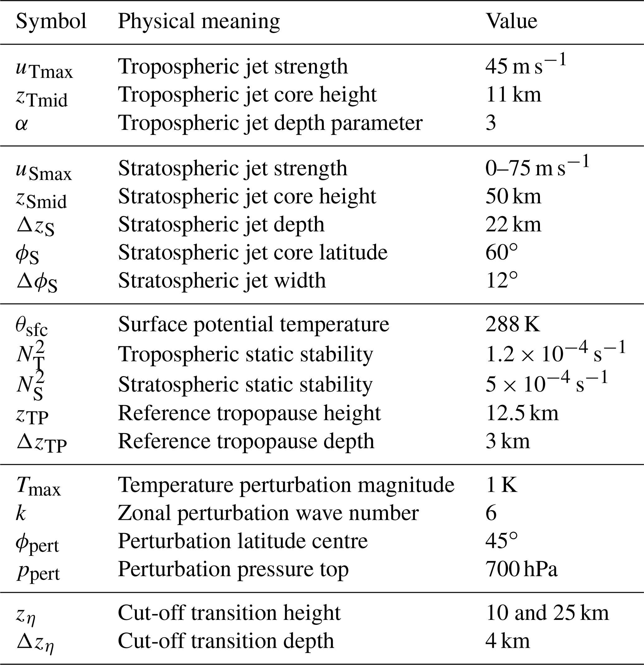
where p₀=1000 hPa and λ is longitude. Table A1 lists the physical parameters and parameter ranges used to define the different basic states used in the present paper.

Table A1 Physical parameters used in the different model experiments.