the Creative Commons Attribution 4.0 License.
the Creative Commons Attribution 4.0 License.
 | 22 Mar 2021
Representation by two climate models of the dynamical and diabatic processes involved in the development of an explosively deepening cyclone during NAWDEX
David L. A. Flack
Ionela Musat
Romain Roehrig
Sandrine Bony
Julien Delanoë
Quitterie Cazenave
Jacques Pelon
The dynamical and microphysical properties of a well-observed cyclone from the North Atlantic Waveguide and Downstream Impact Experiment (NAWDEX), called the Stalactite cyclone and corresponding to intensive observation period 6, is examined using two atmospheric components (ARPEGE-Climat 6.3 and LMDZ6A) of the global climate models CNRM-CM6-1 and IPSL-CM6A, respectively. The hindcasts are performed in “weather forecast mode”, run at approximately 150–200 km (low resolution, LR) and approximately 50 km (high resolution, HR) grid spacings, and initialised during the initiation stage of the cyclone. Cyclogenesis results from the merging of two relative vorticity maxima at low levels: one associated with a diabatic Rossby vortex (DRV) and the other initiated by baroclinic interaction with a pre-existing upper-level potential vorticity (PV) cut-off. All hindcasts produce (to some extent) a DRV. However, the second vorticity maximum is almost absent in LR hindcasts because of an underestimated upper-level PV cut-off. The evolution of the cyclone is examined via the quasi-geostrophic ω equation which separates the diabatic heating component from the dynamical one. In contrast to some previous studies, there is no change in the relative importance of diabatic heating with increased resolution. The analysis shows that LMDZ6A produces stronger diabatic heating compared to ARPEGE-Climat 6.3. Hindcasts initialised during the mature stage of the cyclone are compared with airborne remote-sensing measurements. There is an underestimation of the ice water content in the model compared to the one retrieved from radar-lidar measurements. Consistent with the increased heating rate in LMDZ6A compared to ARPEGE-Climat 6.3, the sum of liquid and ice water contents is higher in LMDZ6A than ARPEGE-Climat 6.3 and, in that sense, LMDZ6A is closer to the observations. However, LMDZ6A strongly overestimates the fraction of super-cooled liquid compared to the observations by a factor of approximately 50.
- Article
(11619 KB) - Full-text XML
-
Supplement
(6247 KB) - BibTeX
- EndNote


Extratropical cyclones are one of the leading hazards in the mid-latitudes, but their projected behaviour under climate change remains uncertain (e.g. Harvey et al., 2012). This uncertainty lies in the location of the extratropical cyclones and the intensity and position of the storm track (e.g. McDonald, 2011; Zappa et al., 2013b) rather than in the total number of extratropical cyclones (e.g. Finnis et al., 2007; Bengtsson et al., 2009; Catto et al., 2011; Zappa et al., 2013b).
Uncertainties in climate simulations can arise from three different factors: model physics, internal variability, and forcings (e.g. Hawkins and Sutton, 2009). Therefore, to determine confidence in future projections, the historical model climate is compared to observations or re-analyses (e.g. Seiler and Zwiers, 2016). Typically, the representation of cyclones in climate models is considered through statistics, e.g. number and frequency (e.g. Zappa et al., 2013a; Seiler and Zwiers, 2016). These studies generally indicate systematic limitations of coarse-resolution models rarely producing explosively deepening cyclones, producing too many weak cyclones, and a storm track that is both too zonal and too far south.
Recently, studies have started to investigate the 3D structure of cyclones (e.g. Catto et al., 2010) and the roles of diabatic heating in climate models (e.g. Willison et al., 2013; Trzeciak et al., 2016; Sinclair et al., 2020). Willison et al. (2013) and Trzeciak et al. (2016) showed that increased resolution, compared to that of the Coupled Model Intercomparison Project (CMIP) models at the time (CMIP5), was required to improve the representation of the diabatic heating and hence representation of the cyclone. This improved representation of diabatic heating could be important as Sinclair et al. (2020) indicated that diabatic processes could become more important in a warming climate. However, fundamental processes linked to extratropical cyclone formation and development need further investigation in global circulation models (GCMs). Fundamental processes linked to factors such as cyclogenesis and cyclone development are hard to examine in full-length free-running climate simulations and could explain a lack of consideration of this to date. Therefore, to examine the representation of the physical processes in cyclone formation and development, different techniques are required. These techniques include running climate model configurations in “weather forecast mode” (e.g. Phillips et al., 2004) or running short ensemble forecasts (e.g. Wan et al., 2014).
The idea of running climate model configurations in “weather forecast mode” culminated in the formation of the Transpose – Atmospheric Model Intercomparison Project (T-AMIP) experiments (Williams et al., 2013). The T-AMIP experiments are primarily used to assess whether any long-term model biases occur within the first few days of the simulations. It was hoped that, if these biases formed early in the climate simulations, model improvements to reduce those biases could be tested with less computational expense (e.g. Williams et al., 2013; Ma et al., 2013). It was further thought this application could help disentangle the origin of the model biases in a more causal way (e.g. Brient et al., 2019). The T-AMIP experiments have considered factors such as cloud cover behind fronts in extratropical cyclones (e.g. Williams et al., 2013); radiative feedbacks (e.g. Williams et al., 2013; Bony et al., 2013; Fermepin and Bony, 2014); 2 m temperature (e.g. Fermepin and Bony, 2014; Ma et al., 2014); precipitation (e.g. Ma et al., 2013; Fermepin and Bony, 2014; Pearson et al., 2015; Li et al., 2018); and stratocumulus (e.g. Brient et al., 2019); and they have been used alongside random-parameter ensembles to determine structural vs. parameter sensitivities (e.g. Sexton et al., 2019; Karmalkar et al., 2019).
The T-AMIP type experiments can also be used as a powerful tool for considering the representation of dynamical processes in climate models. For example, Trzeciak et al. (2016) showed that climate models of resolution T127 (ca. 1.1–1.5∘ at mid-latitudes) can represent deep extratropical cyclones and their tracks well. This good representation was attributed to an increased importance of the diabatic heating compared to lower-resolution simulations. Like Trzeciak et al. (2016), we consider the dynamical representation of extratropical cyclones and the impact of resolution in climate models. However, we focus on a single, well-observed cyclone during the intensive observation period (IOP) 6 of the North Atlantic Waveguide and Downstream Impact Experiment (NAWDEX) field campaign (Schäfler et al., 2018), which is called the “Stalactite” cyclone. This cyclone is initiated from the interaction of two features that occur on sub-grid scales of current climate models. The main deepening phase is characterised by the interaction of the surface cyclone with successive synoptic-scale upper-level troughs. Here we answer the following questions on the representation of the cyclone in climate models to provide further insights into whether climate models are producing cyclones for the correct reasons.
-
How well do climate models represent the two stages of the Stalactite cyclone?
-
What are the relative roles of diabatic and dynamic processes in the development of the Stalactite cyclone?
-
Are there any differences between the two models’ diabatic processes that are related to microphysical properties?
The NAWDEX field campaign occurred in September–October 2016 with the aim of making targeted observations of processes that numerical atmospheric models poorly represent (Schäfler et al., 2018). These observations would then be used to help determine how well the models represent these processes (e.g. Maddison et al., 2019; Oertel et al., 2019). The observations taken during the field campaign allow for an extra question to be asked in this study.
- 4.
Can microphysical observations made during the field campaign give any useful information about the climate model's performance?
To our knowledge, this study is the first time that a climate model is compared with flight data taken during a field campaign without nudging analyses into the simulation, and it is only feasible because of the T-AMIP protocol.
The questions asked here are of particular interest for the Stalactite cyclone as it influences the development of a blocking anticyclone over Scandinavia and marks the transition between a North Atlantic Oscillation (NAO) positive regime and a Scandinavian blocking regime over the North Atlantic European sector. Therefore, it is a particularly useful case to determine the capabilities of our current climate models.
The remainder of this paper has the following layout. The key features of the Stalactite cyclone are discussed in Sect. 2. The GCMs, experimental set-up, observations, and diagnostics are described in Sect. 3. The Stalactite cyclone's representation in the two GCMs is discussed in Sect. 4. A summary is made in Sect. 5.
The Stalactite cyclone corresponds to IOP 6 of the NAWDEX field campaign (Schäfler et al., 2018). It was an explosively deepening cyclone that initially formed at 18:00 UTC 29 September 2016 (Fig. 1a) off the coast of Newfoundland (ca. 45∘ N, 56∘ W; Fig. 1b). Cyclogenesis occurred as a result of the merging of two vorticity maxima at low levels (Fig. 1c). The northern maximum over Newfoundland is formed via baroclinic interaction with an upper-level potential vorticity (PV) cut-off that extended down to the surface like a stalactite (hence the name of the cyclone). The southern maximum corresponds to a diabatic Rossby vortex (DRV). A DRV corresponds to an isolated positive PV anomaly rapidly travelling eastward in a moist and baroclinic region1. To determine if this diabatic precursor is a DRV, we use the criteria set by Boettcher and Wernli (2013). All of the criteria are met in ECMWF analysis, which confirms the identification of a DRV. It was formed on 27–28 September off the coast of Florida and South Carolina (not shown). The DRV was probably produced from a mesoscale convective system, as confirmed by satellite images showing cold brightness temperature (e.g. Fig. 1e).

Figure 1An overview of the Stalactite cyclone. (a) The ECMWF analysis minimum pressure evolution. (b) The track of the Stalactite cyclone (black). The dashed magenta line is the flight path of SAFIRE Falcon-20 flight 6 and the solid is for flight 7. The star and triangle in (a) and (b) represent the timing of panels (c) and (e) and (d) and (f), respectively. (c) The ECMWF analysis of the 250 hPa PV > 2 PVU (contoured) and 850 hPa relative vorticity (shaded) at cyclogenesis (18:00 UTC 29 September), and (d) is like (c) but just before maximum deepening at 12:00 UTC 1 October. The bold lines are to indicate the PV signature of different PV regions interacting with the cyclone. “A” is the upper-level signature of the Stalactite cyclone at that time, “B” is the second PV region to interact with the cyclone, and “C” is the third. The colour scale applies to both (c) and (d). (e) A visible satellite image from MODIS on 29 September indicating the Stalactite cyclone at cyclogenesis. The brightness temperature has been overlaid and saturated at 50 %. (f) The visible satellite imagery from MODIS on 1 October 2016. The satellite images are produced by courtesy of NOAA Worldview (https://worldview.earthdata.nasa.gov/, last access: 1 September 2020).
The two low-level precursors merge into a single cyclonic vorticity maximum in a vortex roll-up by the subsequent analysis (not shown). The initial cyclogenesis phase led to a short deepening stage over 18 h as the cyclone travelled east past Newfoundland. The cyclone underwent a second, more substantial, deepening as a result of an interaction with a large-scale region of high PV at upper levels as the cyclone began to cross the North Atlantic. This region is marked by multiple regions of high PV (“B” and “C” in Fig. 1d) that are successively injected into the upper-level disturbance (“A”) and interact with the Stalactite cyclone. The deepening occurred at a rate of 24.1 hPa in 24 h and so meets the criterion set in Sanders and Gyakum (1980)2 to be classified as an explosively developing cyclone. The explosive deepening occurred between 18:00 UTC 30 September and 18:00 UTC 1 October (Fig. 1a). During the interaction with the second large-scale trough cyclonic wave breaking occurred and the cyclone re-curved towards Greenland (Fig. 1b). On reaching the coast of Greenland cyclolysis (i.e. cyclone decay) occurred; the cyclone had filled in by 00:00 UTC 4 October. The cyclone posed an interesting challenge for operational numerical weather prediction models as the cyclone participated in a regime transition from an NAO positive regime to a Scandinavian blocking regime which dominated the North Atlantic European sector for the rest of the field campaign (e.g. Schäfler et al., 2018; Maddison et al., 2019). Correspondingly, there was a reduction in the forecast skill (Schäfler et al., 2018). To determine whether the climate models are correctly simulating the Stalactite cyclone three criteria are developed from its life cycle.
-
Initial cyclogenesis occurs as a result of the merger of a DRV and another near-surface cyclonic vortex associated with baroclinic interaction with an upper-level PV cut-off.
-
A main deepening phase associated with large-scale troughs is present.
-
There is a minimum pressure deepening rate of 24 hPa in 24 h during the secondary deepening phase.
If all of these criteria are met, then the climate models are able to correctly represent the Stalactite cyclone. The climate models and experimental set-up used are discussed in the following section.
In this section, we discuss the model set-up and experimental protocol of the T-AMIP experiments (Sect. 3.1), the observations (Sect. 3.2), and diagnostics considered (Sect. 3.3). We also compare our simulations against the European Centre for Medium Range Weather Forecasting (ECMWF) analysis as a consistent baseline with the initiation state.
3.1 Models and experimental set-up
We use two atmospheric GCMs: ARPEGE-Climat 6.3 (hereafter ARPEGE) and LMDZ6A (hereafter LMDZ) of the CNRM-Cerfacs (Centre National de Recherches Météorologiques – Centre Européen de Recherche et de Formation Avancée en Calcul Scientifique; Voldoire et al., 2019) and IPSL (Institut Pierre Simon Laplace; Boucher et al., 2020) climate models: CNRM-CM6-1 and IPSL-CM6A, respectively. Both climate models recently contributed to CMIP6 (Eyring et al., 2016), and here we make use of the same model versions and configurations. Table 1 shows the details of the model configurations used. These GCMs are run in “weather forecast mode” to represent T-AMIP-style experiments. Hereafter, ARPEGE-LR (-HR) and LMDZ-LR (-HR) refer to low-resolution (high-resolution) runs of the two models.
(Roehrig et al., 2020)(Hourdin et al., 2020)Piriou et al. (2007)Guérémy (2011)Rochetin et al. (2014)Mlawer et al. (1997)Mlawer et al. (1997)Fouquart and Bonnel (1980); Morcrette et al. (2008)Fouquart and Bonnel (1980)Lopez (2002)Madeleine et al. (2020)Hourdin et al. (2019)Table 1Model descriptions with key parameterisations and hindcast resolutions.

The LMDZ-HR configuration utilises its zoom function, in which the resolution over part of the domain is increased compared to the rest in a variable resolution configuration. Here the zoomed domain is centred at 55∘ N, 40∘ E with a resolution equivalent to 0.33∘. The resolution decreases away from the centre, resulting in a resolution of approximately 0.5∘ over the North Atlantic and 1.1∘ elsewhere.
For ARPEGE, microphysics state variables and turbulent kinetic energy were initialised to zero, and aerosols are prescribed from a present-day climatology. On the other hand, in the LMDZ model, state variables not defined in the analysis are set to zero, alongside the aerosols. All hindcasts are performed out to a lead time of T+10 d. Furthermore, all hindcast output data are interpolated onto a pressure grid in the vertical, every 25 hPa, from 1000 to 100 hPa. Output is also produced using the CFMIP (Cloud Feedback Model Intercomparison Project) Observation Simulator Package (COSP; Bodas-Salcedo et al., 2011) for radar reflectivities from CloudSat to be compared with the observed aircraft-borne radar reflectivities from the NAWDEX field campaign.
The hindcasts are initiated at 00:00 UTC 29 September and 1 October 2016 from the ECMWF analysis (including sea surface and ice cover). The first initiation time is used to examine the entire life cycle of the Stalactite cyclone; the second is used for observational comparisons (Sect. 4.4) to ensure similar cyclone structure and position to reality. We restrict the number of hindcasts to take into account the impact of the overall synoptic situation at the time being largely unpredictable (e.g. Schäfler et al., 2018). Initial shock (e.g. Klocke and Rodwell, 2014) is checked for but is not significant. However, as a precautionary measure, we do not analyse hindcasts prior to T+18 h.
3.2 Observations
During the NAWDEX field campaign, the French SAFIRE Falcon aircraft operated from 1–15 October (Schäfler et al., 2018). The SAFIRE Falcon made two flights to observe the Stalactite cyclone on 2 October 2016: F6 (towards Greenland) and F7 (south of Iceland; Fig. 1b). The second flight (F7) was directly into the cyclone in the ascending branch of the associated warm conveyor belt. The first flight (F6) considered the warm conveyor belt outflow. In the main paper we focus on F7. The first leg of F7 (the most easterly one) was chosen because there was an overpass with CloudSat–CALIPSO track at 14:09 UTC which allows us to assess observation uncertainties by comparing airborne and satellite measurements. The payload on board the SAFIRE Falcon included a 95 GHz Doppler cloud radar and a high-spectral-resolution Doppler lidar capable of measuring at 355, 532, and 1064 nm (e.g. Delanoë et al., 2013). Measurements by these two instruments allow for the retrieval of ice water content (IWC) thanks to the variational algorithm of Delanoë and Hogan (2008), updated by Cazenave et al. (2019). The combination of radar and lidar allows for the identification of the phase of the particles to be identified (e.g. super-cooled liquid, ice, liquid, etc.) using principles outlined in Delanoë and Hogan (2010). Furthermore, Doppler-derived wind speeds and radar reflectivities are also used. Retrievals from radar products only (RASTA) and a combined radar and lidar product (RALI) are used to account for uncertainty in the measurements. Complementary information on the flight and measurements is available in Blanchard et al. (2020).
3.3 Vertical motion and baroclinic conversion budgets
Extratropical cyclone evolution can be considered through many methods, for example, the surface pressure tendency equation (e.g. Fink et al., 2012); through a potential vorticity framework (e.g. Davis et al., 1993); or the quasi-geostrophic (QG) vertical motion (ω) equation (e.g. Sinclair et al., 2020). Here, as in Sinclair et al. (2020), we consider the evolution through the QG ω equation. We also consider the energetics of the cyclone through the baroclinic conversion (BC).
The QG ω equation, which includes diabatic heating and the β term, can be written in terms of the so-called Q vector following Hoskins et al. (1978) and Hoskins and Pedder (1980). We use the formulation of Holton (2004) that includes the diabatic heating too:
for
where σ is the static stability (obtained by temporally averaging the temperature across the lifetime of the Stalactite cyclone), f0 is a reference coriolis parameter, β is the beta term in the coriolis forcing, p is the pressure, R is the specific gas constant, cp is the specific heat, J is the rate of heating per unit mass, ug is the geostrophic wind vector, T is the temperature, x and y are the positions in the meridional and zonal directions, respectively, and ωQG is the vertical velocity obtained from inverting the QG ω equation.
Equation (1) allows us to distinguish between the dynamical and diabatic contributions to the vertical motion in the cyclone. Physically, the Q vector and the β terms represent the dynamical components of the flow and the Laplacian of the rate of heating per unit mass represents the diabatic heating.
To solve Eq. (1) the 3D Laplacian is inverted over the region 35–75∘ N and 70∘ W–0∘ E using Liebmann successive over-relaxation with boundary conditions such that ω is zero at 1000 hPa, 100 hPa, and all horizontal boundaries. The vertical motion is computed every 25 hPa in the vertical. Comparisons of modelled ω and ωQG occur in Sect. 4.3. We also invert the dynamic and diabatic components of the ωQG (ωdyn, ωdiab) to gain further insights into the development of the cyclone.
Vertical velocity occurs in different key terms of the classical equations for the development of extratropical cyclones. We adopt the energetic framework and compute the baroclinic conversion from eddy potential energy to eddy kinetic energy within the extratropical cyclone (e.g. Orlanski and Katzfey, 1991; Rivière and Joly, 2006). The baroclinic conversion is proportional to the vertical heat flux and can be written as
where , ps is the surface pressure, and θ is the potential temperature. Primes denote the difference from the 5 d temporal average of that quantity centred over the life cycle of the Stalactite cyclone. The results are insensitive to the definition of the temporal average provided it is made over an interval equal to or longer than the life cycle of the cyclone to suppress the cyclone's signal. The baroclinic conversion term is mainly positive in areas following the cyclone trajectory (Rivière and Joly, 2006; Rivière et al., 2015).
We approximate BC by replacing the vertical velocity by its QG formulation in Eq. (1), denoted as ωQG, and keeping θ′ unchanged. The approximated is decomposed into its dynamic and diabatic components (respectively and ) by inverting the corresponding components of vertical velocity in Eq. (1) separately.
Throughout this section the dynamical and diabatic representation of the Stalactite cyclone is discussed. The minimum pressure evolution and cyclone track are considered in Sect. 4.1. An in-depth consideration of the cyclogenesis and development occur in Sect. 4.2 and 4.3, respectively. The two climate models are compared to the flight observations and discussed in relation to diabatic heating in Sect. 4.4.
4.1 Pressure evolution and track
The representation of the Stalactite cyclone is first considered via an overview of the cyclone through its track and minimum sea level pressure evolution (Fig. 2). All hindcasts produce a rapidly deepening cyclone: slightly more than 24 hPa in 24 h in HR hindcasts and slightly less than 24 hPa in 24 h in LR hindcasts. However, this deepening is delayed by 24 h compared to the analysis in the LR simulations. Furthermore, the initial cyclogenesis is not as intense in LR simulations compared to the analysis. This weaker cyclogenesis results in an initially weaker cyclone compared to the analysis in both models (Fig. 2a). However, the explosive deepening in LMDZ-LR compensates for the lack of initial deepening. Conversely, ARPEGE-LR has the same secondary deepening strength as the analysis, so it produces a weaker cyclone. The HR hindcasts both have an improved representation of the initial cyclogenesis, so they show more realistic cyclone development in terms of pressure evolution.

Figure 2An overview of the Stalactite cyclone: (a) the minimum pressure evolution and (b) the cyclone track. The ECMWF analyses are in black, LMDZ hindcasts in red, and ARPEGE hindcasts in blue. The LR hindcasts are the solid lines, and the HR hindcasts are dashed. All hindcasts are initiated at 00:00 UTC 29 September 2016.
The cyclone track also differs from the analysis. The difference occurs 18 h after the start of initialisation. The two LR hindcasts produce a track that is too far south and has a later re-curvature, so the cyclone track occurs further east compared to the analysis and HR hindcasts (Fig. 2b). The eastward shift in the track agrees with global weather forecasts prior to 29 September 2016 (e.g. Maddison et al., 2020). Given the rapid divergence of the forecast track from the analysis, differences in the cyclogenesis could be one aspect leading to the track occurring too far east as argued later in that section. The cyclogenesis being important for the cyclone track is also corroborated by the track representation having improved (i.e. no eastward shift) after the cyclone appears in the initial conditions (not shown).
The main differences to the representation of the Stalactite cyclone compared to the analysis, on initial inspection, appear to be within the cyclogenesis phase of the cyclone and the different deepening rate of LMDZ compared to ARPEGE and the analysis. These two aspects are examined further within the following subsections.
4.2 Cyclogenesis
The cyclogenesis of the Stalactite cyclone occurs on the mesoscale as the merging of two low-level vorticity precursors: a DRV coming from the subtropics and a vortex located further north baroclinically interacting with an upper-level PV cut-off (Fig. 1c). In the present section we analyse the representation of the two precursors and their subsequent merging in the different simulations. The same vorticity fields as in Fig. 1c are shown in Fig. 3 for the different simulations. Figures 4 and 5 show the baroclinic conversion at T+18 h for both ARPEGE and LMDZ, respectively, and help identify the mechanisms behind the two precursors for the Stalactite cyclone; there is a close relationship between the two components as the dynamics and diabatic processes are tightly coupled.
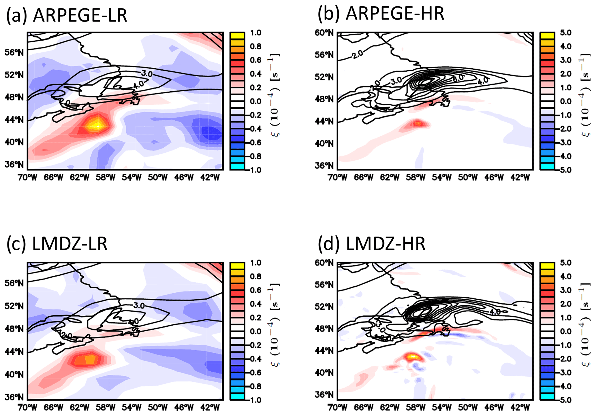
Figure 3Hindcasts for the cyclogenesis of the Stalactite cyclone at 18:00 UTC 29 September (T+18 h) for hindcasts initiated at 00:00 UTC 29 September. The 250 hPa PV above 2 PVU (contoured every 1 PVU) and the 850 hPa relative vorticity (shaded) for (a) ARPEGE-LR, (b) ARPEGE-HR, (c) LMDZ-LR, and (d) LMDZ-HR. The colour scale is different between LR and HR runs.
4.2.1 The diabatic Rossby vortex
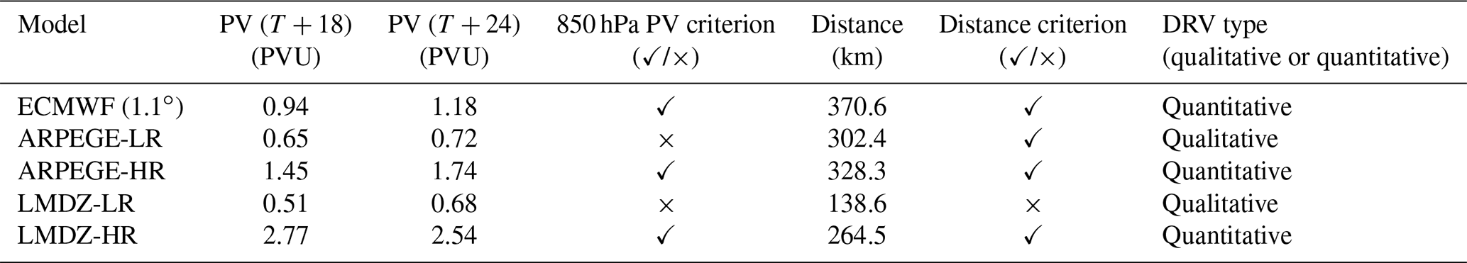
Criteria of DRV introduced by Boettcher and Wernli (2013) have been analysed in the different simulations. The two HR hindcasts fit all the criteria of a DRV, producing a stronger DRV than the ECMWF, which shows that 50 km grid spacing is enough to represent the DRV. The LR hindcasts meet all but two of the criteria of Boettcher and Wernli (2013): the PV intensity (for both) and propagation speed (LMDZ-LR; Table 2). However, it is encouraging to see that the LR hindcasts produce a qualitative representation of a DRV despite the coarse resolution of the models and the mesoscale nature of this self-sustaining phenomenon. The identification of the southern precursor as a DRV is confirmed by the baroclinic conversion of Figs. 4 and 5 which show that the diabatic component is almost equal to the total in the vicinity of the vortex and that the dynamical component is negligible. The DRV is more active in LMDZ-LR compared to ARPEGE-LR as the associated heating rate reaches higher values in LMDZ-LR compared to ARPEGE-LR (cf. Figs. 4c and 5c). Vertical cross sections of the heating rates across the DRV indicate that its structure extends throughout the atmospheric column (Fig. S1 in the Supplement) confirming the impression left by the satellite image (Fig. 1e).
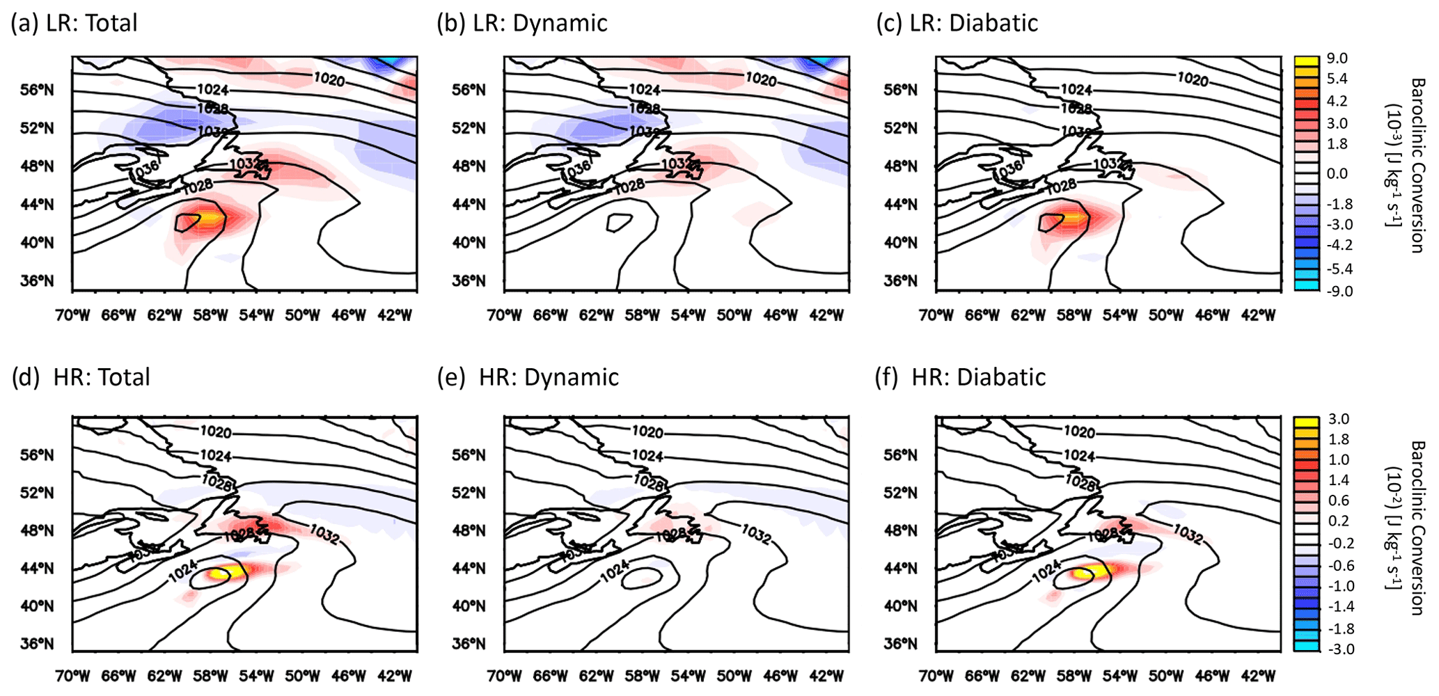
Figure 4Vertically averaged baroclinic conversion between 850 and 300 hPa (shaded) and mean sea level pressure (contoured) at 18:00 UTC 29 September 2016 (T+18 h from hindcast initiation at 00:00 UTC 29 September 2016) for ARPEGE hindcasts. (a–c) ARPEGE-LR hindcast and (d–f) ARPEGE-HR hindcast. (a, d) Total (dynamic plus diabatic) baroclinic conversion, (b, e) baroclinic conversion from dynamical processes, and (c, f) baroclinic conversion from diabatic processes. The colour scales refer to each row.
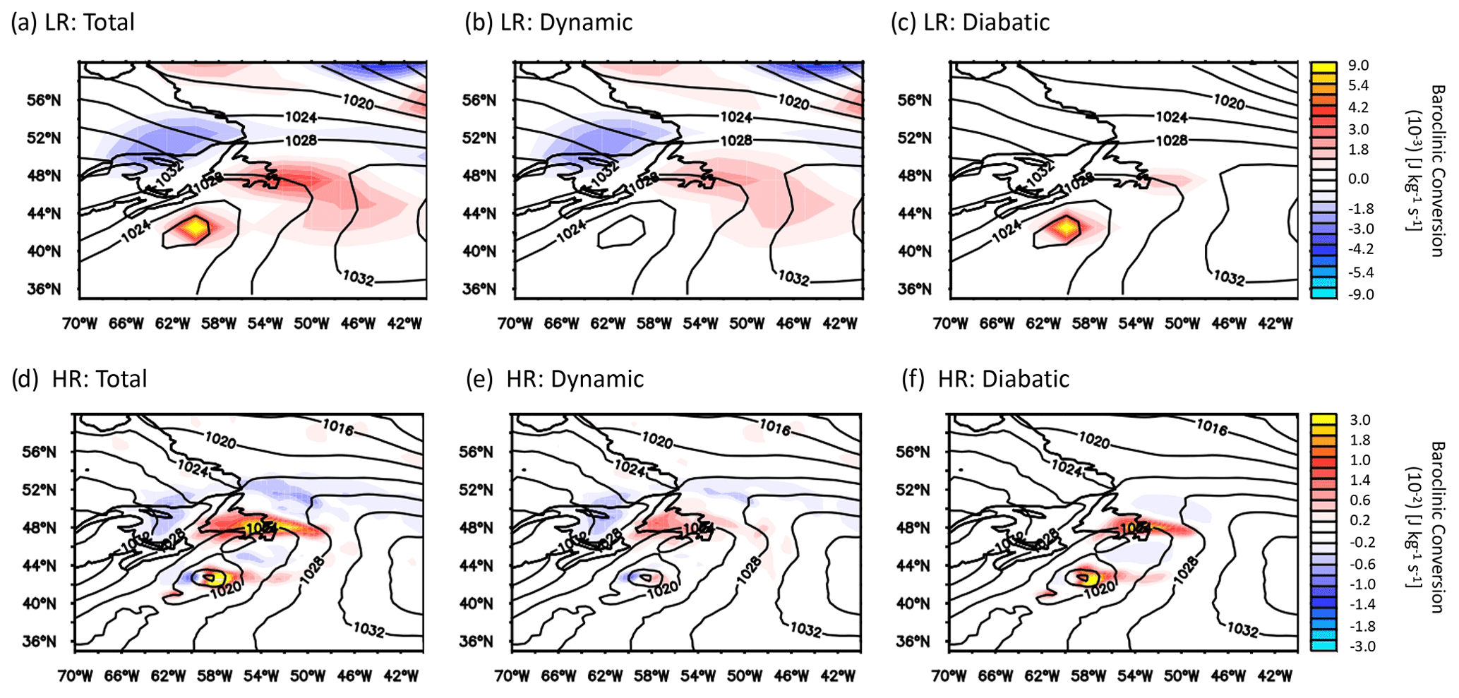
Figure 5As in Fig. 4 but for LMDZ-LR (and -HR) hindcasts.
Table 2Distance and PV criteria from Boettcher and Wernli (2013) for identifying DRVs between T+18 and T+24 from the hindcast initialised at 00:00 UTC 29 September. The PV criterion is based on a minimum PV value when averaged at the minimum MSLP location and the eight surrounding grid boxes, which is set to 0.8 PVU. The distance criterion is based on a minimum distance travelled by the vortex in 6 h, which is 250 km. When the threshold is reached a ✓ is present, otherwise a ×. The DRV is described as quantitative if all the thresholds are reached and qualitative otherwise. Only criteria for which at least one of the hindcasts do not meet the criteria are shown.
4.2.2 Formation of the northern precursor via baroclinic interaction with the PV cut-off
More important differences appear between LR and HR runs in the representation of the northern precursor. In the LR hindcasts the vorticity of the northern precursor is much smaller than the vorticity of the DRV precursor (reduced by factors of 2.4 in ARPEGE-LR and 3.3 in LMDZ-LR), whereas it is only slightly smaller in HR runs (ratio of 1.6 in ARPEGE-HR and 1.3 in LMDZ-HR). Furthermore, the LR runs (Fig. 3a, c) have a more zonal PV cut-off than in the analysis (Fig. 1c) and in the two HR runs (Fig. 3b, d). Also, the low-level northern vorticity maximum moves to the east of the cut-off in the HR runs and analysis, which is typical of strong baroclinic interaction, whereas it stays to the south of the cut-off in LR runs (Fig. 3a and c).
Unlike the DRV, the northern precursor is a mixture of diabatic and dynamic processes, as shown by the baroclinic conversion rates of Figs. 4 and 5. The vertical cross sections of Fig. 6 show that the dynamical component is mainly centred at upper levels but with an equivalent barotropic structure. This suggests that the northern precursor is forced by the vertical velocity associated with the PV cut-off, which is characteristic of type-B cyclogenesis (Petterssen and Smebye, 1971). In LR hindcasts the dynamical forcing has a smaller vertical extent and is more spread out than the HR hindcasts. The dynamical forcing in LR hindcasts is located further east than the diabatic forcing (Fig. 6b and c), while the two forcings are more superimposed in HR hindcasts (Fig. 6e and f and Fig. S2 for ARPEGE). Both forcings increase with resolution by a factor of more than 5 in the two models. However, the peak values of the diabatic baroclinic conversion exhibit a larger increase than those of the dynamical baroclinic conversion during the formation of the northern precursor (Figs. 5b, c, e, f and 6b, c, e, f).
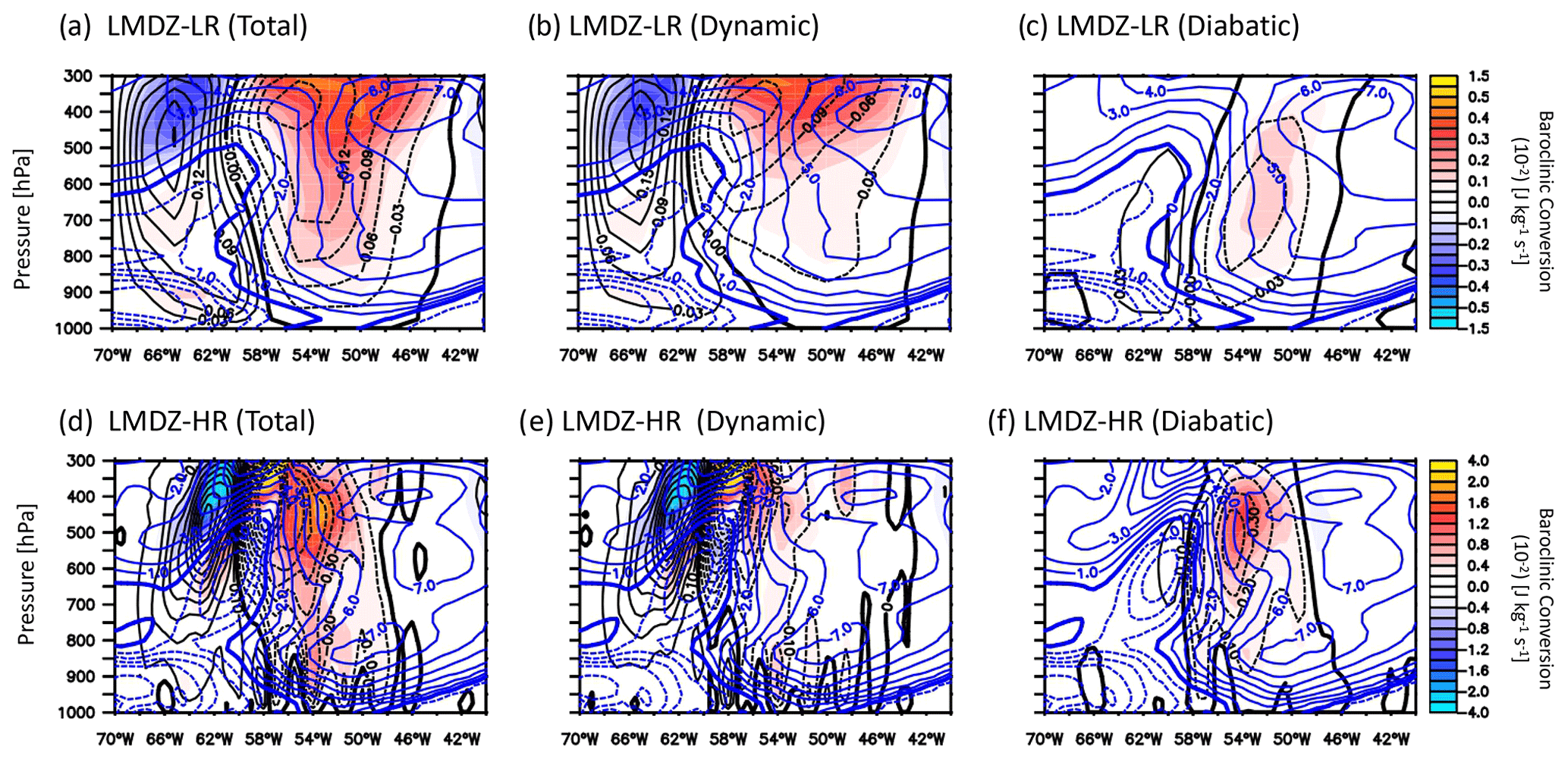
Figure 6A vertical cross section averaged across the northern precursor in the LMDZ hindcasts at 18:00 UTC 29 September 2016 (T+18 h). The baroclinic conversion (shaded), potential temperature anomaly (blue contours), and inverted ω (black contours) for (a, d) total baroclinic conversion, (b, e) the baroclinic conversion due to dynamic processes only, and (c, f) the baroclinic conversion from diabatic processes. (a–c) LMDZ-LR and (d–f) LMDZ-HR. Note that the colour scales and contours are different between the LR and HR runs.
To conclude, the northern precursor is rather poorly represented in LR compared to HR hindcasts because the less intense, and more spatially diluted, PV inside the cut-off induces a weaker dynamical forcing. An additional factor is the more active diabatic forcing in HR hindcasts in the vicinity of the northern precursor. So whilst both the dynamical and diabatic terms improve with resolution, it is difficult to determine which component matters most.
4.2.3 Merging of the two precursors
For the hindcasts shown here, the merger of these two different precursors differs in timing from the analysis and between resolutions. The HR configurations (although delayed by 6 h compared to the ECMWF analysis) merge the DRV and upper-level dynamical precursor 12–18 h earlier than the LR runs (not shown). For LMDZ-LR there is even no merging of the two precursors. The delay or absence of interaction between the two precursors likely has an impact on the track of the cyclone which was systematically located too far east in the LR runs (Fig. 2b) as the precursor merger starts the more northward movement of the cyclone in the track. This is understandable by the fact that the earlier merging is associated with a stronger upper-level forcing which is required for a cyclone to move northward perpendicularly to the jet axis (Coronel et al., 2015). There are two factors to explain the delayed or missed merging. One is the more rapidly eastward propagation of the DRV in HR than LR runs (Fig. 3; Table 2), which is consistent with stronger latent heating in the former runs. The second is that the low-level northern precursor and the upper-level cut-off are moving less rapidly eastward in HR runs (not shown). This can be partly explained by the difference in longitude of the dynamical forcing between LR and HR hindcasts (compare Fig. 6b and e). The more rapid propagation of the DRV and less rapid motion of the northern precursor explain why the DRV is more able to catch up to the northern precursor in HR runs as in the analysis.
To conclude on cyclogenesis, the LR hindcasts struggle to correctly represent the initiation of the cyclone because they miss the initial deepening of the northern small-scale low-level vortex and the roll-up of the merging of the two low-level vortices around the PV cut-off. However, the unexpected result is that the LR hindcasts are able to reproduce the behaviour of the DRV rather well, albeit with a smaller propagation speed.
4.3 Main deepening
The main focus of this section is the main deepening stage of the Stalactite cyclone. Like the cyclogenesis phase, the main deepening phase is considered by analysing the baroclinic conversion. The baroclinic conversion is considered either as an average over a 1010∘ area centred on the minimum pressure of the Stalactite cyclone (Fig. 7) or from its local maximum (Fig. S3). The averaged QG baroclinic conversion roughly recovers 60 %–70 % of the amplitude of that directly calculated from the model ω (Fig. 7) throughout the cyclone life cycle. In addition, the model and QG baroclinic conversions are very similar in the timing, evolution, structure (not shown), and maximum peaks (Fig. S3). This good correspondence provides confidence in our inversions and results.
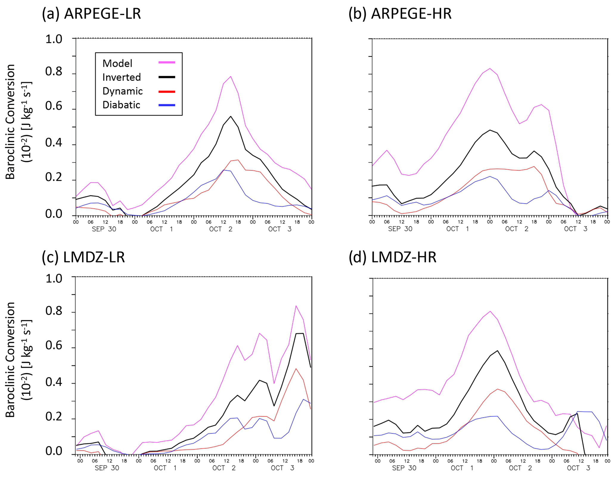
Figure 7The evolution of the average baroclinic conversion in a 10 ∘ × 10 ∘ box around the minimum pressure of the Stalactite cyclone for (a) ARPEGE-LR, (b) ARPEGE-HR, (c) LMDZ-LR, and (d) LMDZ-HR. The magenta line is for the baroclinic conversion calculated with the model ω, the black line is the total inverted ω, the red line is the inverted ω from dynamical processes, and the blue line is the inverted ω from diabatic processes. All hindcasts were initiated at 00:00 UTC 29 September 2016, and average times are defined, subtly, differently in LMDZ and ARPEGE, hence the 1.5 h extension in LMDZ plots. Maximum point values of baroclinic conversion are shown in Fig. S3.
In the cyclone average values (Fig. 7) the two stages of cyclone development are well separated: (i) the initial cyclogenesis stage occurring on 29–30 September (Sect. 4.2) and (ii) the main development stage that is dominated by the presence of a large-scale trough and an explosively developing cyclone. The initiation stage is clearly dominated by diabatic processes. During the main deepening stage the dynamical processes begin to be more important, and more so in the HR hindcasts compared to the LR hindcasts. In the HR runs the dynamical term is even larger than the diabatic term during the whole main deepening stage. The delay in the dynamical processes compared to diabatic processes is particularly clear in LR hindcasts, suggesting a delayed forcing by the large-scale upper-level trough. Therefore, there is an increased importance of the dynamic term relative to the diabatic term with increased resolution. This ratio consistency is true for both the maximum (Fig. S3) and average values (Fig. 7) in both models and lead times. Furthermore, the ratio consistency in the main deepening stage disagrees with the previous studies of Willison et al. (2013) and Trzeciak et al. (2016). However, for the northern precursor at cyclogenesis we do agree with their studies.

Figure 8The 250 hPa PV (shaded) and mean sea level pressure (contoured) during the maximum deepening phase of the Stalactite cyclone. (a–c) 00:00 UTC 1 October 2016 and (d–f) 12:00 UTC 1 October 2016. (a, d) ECMWF analysis, (b, e) ARPEGE-LR hindcast, and (c, f) ARPEGE-HR hindcast. All hindcasts were initiated at 00:00 UTC 29 September 2016, and the colour scale applies to all plots. LMDZ-LR(-HR) plots at the same time are shown in Fig. S4.
Considering the dynamical processes in more detail (Figs. 8 and S4) helps to indicate the reason for the delay in the maximum deepening in the LR hindcasts compared to the analysis and the HR hindcasts. On 1 October at 00:00 UTC an upper-level PV signature is clearly visible above the surface cyclone in HR hindcasts, while in the LR hindcast the cyclone is still mainly a DRV. The PV injection coming from the large-scale region of high PV, located to the north-east, into the upper-level disturbance interacting with the surface cyclone is delayed in the hindcasts. In the analysis some PV injection has already occurred (Fig. 8a) but is just starting in the HR runs (Fig. 8c). The situation in ARPEGE-HR on 1 October at 12:00 UTC (Fig. 8f) resembles more that of the analysis approximately 6 h earlier (not shown), with the cyclonic wave breaking being more advanced in the ECMWF analysis (Fig. 8d). Several studies have shown that the PV of the upper-level trough baroclinically interacting with a surface extratropical cyclone tends to advect the cyclone polewards (Rivière et al., 2012; Oruba et al., 2013; Coronel et al., 2015). Therefore, the earlier non-linear interaction of the cyclone with the large-scale upper-level PV reservoir and the earlier roll-up of the two features around each other explain the earlier deviation of the cyclone track to the north and the more westward position of the track in the analysis than in the hindcasts. For the HR hindcasts the delay is a maximum of 6 h and the eastward shift is minimal, while for LR hindcasts the delay is about 24 h and the eastward shift is more marked.
4.4 Interpretation of the difference between the models and comparison with aircraft observations
As previously said, to have cyclone features roughly at the same place in the models as in the observations, for a clean comparison, simulations initiated at 00:00 UTC 1 October 2016 are analysed in the present section.
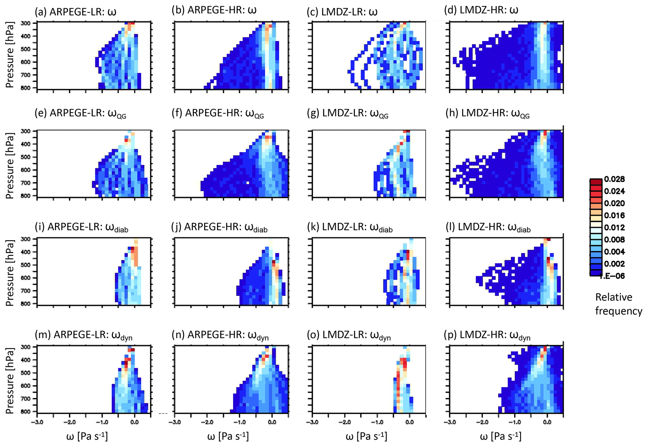
Figure 9Bivariate histograms of vertical velocity vs. pressure in a 6∘ × 6∘ box around the minimum pressure during the mature stage of the cyclone around maximum depth (ca. 12:00 UTC 2 October 2016; T+33–36 h) for (a–d) modelled ω, (e–h) ωQG, (i–l) ωdiab, and (m–p) ωdyn and for (a, e, i, m) ARPEGE-LR, (b, f, j, n) ARPEGE-HR, (c, g, k, o) LMDZ-LR, and (d, h, l, p) LMDZ-HR. The colour scale applies to all plots. The hindcasts were initiated at 00:00 UTC 1 October 2016.
4.4.1 Diabatic heating in the models
To more deeply investigate the relative contributions of dynamics and diabatic components, as well as to assess potential differences between the models, Fig. 9 shows distributions of vertical velocities around the cyclone centre for hindcasts initiated at 00:00 UTC 1 October 2016, but similar results occur for the hindcasts initiated at 00:00 UTC 29 September 2016 (not shown). Figure 9 first shows that the distribution of the model ω is rather well represented by its QG approximation ωQG (Fig. 9a–d and e–h). Only some peak values of model ω near −2 Pa s−1 for LMDZ-LR are missing in ωQG. Second, both vertical velocities increase with increased resolution (Fig. 9a, c, e, g and b, d, f, h). Distributions of ωQG are rather similar in ARPEGE-LR and LMDZ-LR, but the relative contributions of dynamic and diabatic parts differ between the two runs. There are more frequent strong ascents of the diabatic component for LMDZ-LR than ARPEGE-LR (Fig. 9i, k), while the dynamical component partly offsets this difference (Fig. 9m, o). In HR hindcasts, there are the largest values of ωQG in LMDZ-HR compared to ARPEGE-HR (Fig. 9f, h) which is mainly due to the diabatic term.
To conclude, diabatic processes have a stronger impact on vertical velocities in LMDZ than ARPEGE, and the diabatic heating in the former model is stronger than in the latter. The terms that dominate the heating profiles both in ARPEGE and LMDZ are the large-scale condensational heating and convective terms (not shown). Thus, it is likely that observations of microphysical properties of the Stalactite cyclone could be used to qualitatively determine which model has the better heating rates or structure. These comparisons are considered next.
4.4.2 Microphysical properties in the models and in observations
To determine whether observations of microphysical properties from field campaign flights can provide information on the underlying diabatic heating, the Stalactite cyclone hindcasts are compared with flight F7 (Fig. 1b) of the SAFIRE Falcon during the NAWDEX field campaign. To ensure a fair comparison, the observation data have been linearly interpolated onto the model grid, and a nearest-neighbour approach has been used to convert the model onto the flight track. Observed IWC is compared against “potential” IWC (cloud ice plus snow) and “maximum” IWC (cloud ice plus snow plus liquid water content, LWC) to take super-cooled liquid into account.
The wind speeds in the cyclone are well represented in all hindcasts with there only being a small shift in the probability density function toward smaller values by less than 5 m s−1 (not shown). This comparison provides confidence in the large-scale features of the cyclone. Therefore, microphysical features can be further considered. Figure 10 shows bivariate histograms of the IWC for F7 from two observation platforms: RASTA (Fig. 10a) and RALI (Fig. 10f). There are larger values of IWC in RASTA compared to RALI because the lidar (being sensitive to smaller ice particles and smaller quantities of ice) information in RALI leads to a reduction of IWC compared to RASTA. Both platforms show the same shape with increasing values of IWC to around 600 hPa and then a uniform distribution until around 800 hPa, below which the instruments no longer detect ice clouds. The two retrieved IWC histograms provide an indication of uncertainty in the observations, which is useful to be compared with model outputs.
The model contribution to Fig. 10 consists of four rows: the first two rows show “potential” IWC, while the last two show “maximum” IWC. Comparing the first two rows (Fig. 10b–e and g–j) with the observations shows an underestimation of the model IWC. This underestimation is by a factor of 3–4, similar to what Rysman et al. (2018) found when comparing observations and Weather Researching and Forecasting (WRF) model simulations of Mediterranean systems. Furthermore, the peak of the model IWC distribution occurs at 700–750 hPa, 100–150 hPa lower than in the observations. There are small improvements with resolution: the HR simulations have a larger IWC throughout, particularly aloft and in the maximum values. Furthermore, there are differences between the models. The first difference is that the IWC values of LMDZ-LR are more dispersed than those of ARPEGE-LR, suggesting a larger number of ice clouds at this altitude in LMDZ-LR (Figs. 10b, d, g, i; 11a, b). The greater values at upper levels in LMDZ are more in line with the values given by the observations than ARPEGE (cf. Fig. 10a–j). However, although LMDZ may be better at representing the IWC at upper levels, the overall shape of the distribution is better in ARPEGE compared to LMDZ. Indeed, the decreased IWC from 600 to 300 hPa is better represented in ARPEGE. Applying the observation mask to the models (Fig. 10g–j) brings the frequencies more in line with the observations compared to those without the mask by removing all the lowest values seen in the no-mask statistics. This is due to instruments not being sensitive to very small IWC, and also the models do not create discontinuities in IWC between cloudy and clear-sky regions. The comparisons between the mask (Fig. 10g–j) and no-mask (Fig. 10b–e) values implies that there are very small IWC values in the model outside of the observed region (particularly for ARPEGE-LR), indicating the horizontal structure of the cyclone is reasonable.

Figure 10Bivariate histograms of ice water content vs. pressure for F7 for (a) RASTA observations (radar only), (f) RALI (radar plus lidar) observations, (b–e) hindcast output using “potential” ice water content (cloud ice plus snow) without applying a mask to the observations, (g–j) hindcast output of “potential” ice water content with the observation mask applied, (k–n) hindcast for “maximum” ice water content (ice water content plus liquid water content) without the observation mask applied, and (o–r) hindcast of “maximum” ice water content with the observation mask applied for (b, g, k, o) ARPEGE-LR, (c, h, l, p) ARPEGE-HR, (d, i, m, q) LMDZ-LR, and (e, j, n, r) LMDZ-HR. The hindcast data are initiated at 00:00 UTC 1 October 2016 and use the nearest grid point to the flight path from the two times surrounding the flight path (12:00 and 15:00 UTC 2 October 2016; T+36–39 h). The flight occurred from 13:00–16:00 UTC. The colour scale applies to all panels, and the histograms have been normalised by all points.
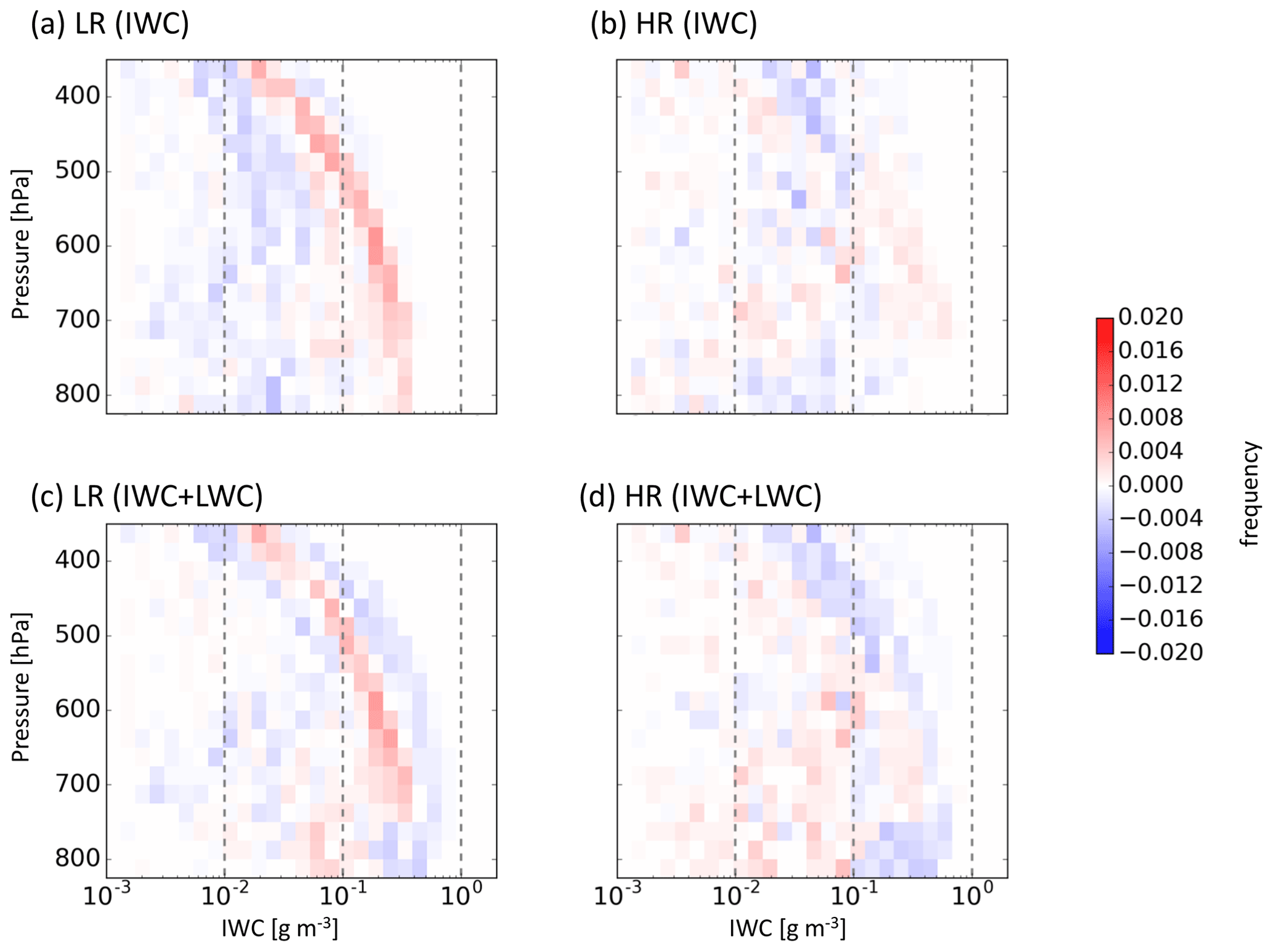
Figure 11Difference bivariate histograms for F7 of ice water content vs. pressure between ARPEGE and LMDZ for (a) LR differences in “potential” ice water content (cloud ice plus snow) only (Fig. 10b–d), (b) HR differences in “potential” ice water content only (Fig. 10c–e), (c) LR differences in “maximum” ice water content (ice water content plus liquid water content) (Fig. 10k–m), and (d) HR differences in “maximum” ice water content (Fig. 10l–n). Reds refer to ARPEGE having a larger quantity and blues for LMDZ. The colour scale applies to all panels. The hindcasts are initiated at 00:00 UTC 1 October 2016 and use the nearest grid point to the flight path from the two times surrounding the flight path (12:00 and 15:00 UTC 2 October 2016; T+36–39 h).
Is the underestimated IWC in the models due to the underestimated liquid-to-solid transition for cold temperatures or to the underestimation of condensates as a whole? To answer this question the LWC below 273 K is added to the IWC to create the last two rows (“maximum” IWC; Fig. 10k–r). Adding the LWC makes limited difference to either of the ARPEGE hindcasts (Fig. 10k, l, o, p), suggesting that either there are fewer LWC points added or the LWC points added have a small magnitude. On the other hand, adding LWC into the LMDZ definition drastically changes the shape and increases the values of total IWC at lower levels (Fig. 10m, n, q, r). The LMDZ distributions have been changed to the extent that the shape now shows more agreement with the observations than when the LWC was not taken into account. These changes in LMDZ are also apparent in Fig. 11, although the model difference is reduced at increased resolution (Fig. 11c and d). The much larger “maximum” IWC in LMDZ compared to ARPEGE over all the levels is consistent with the larger diabatic heating shown in Fig. 9e–h.
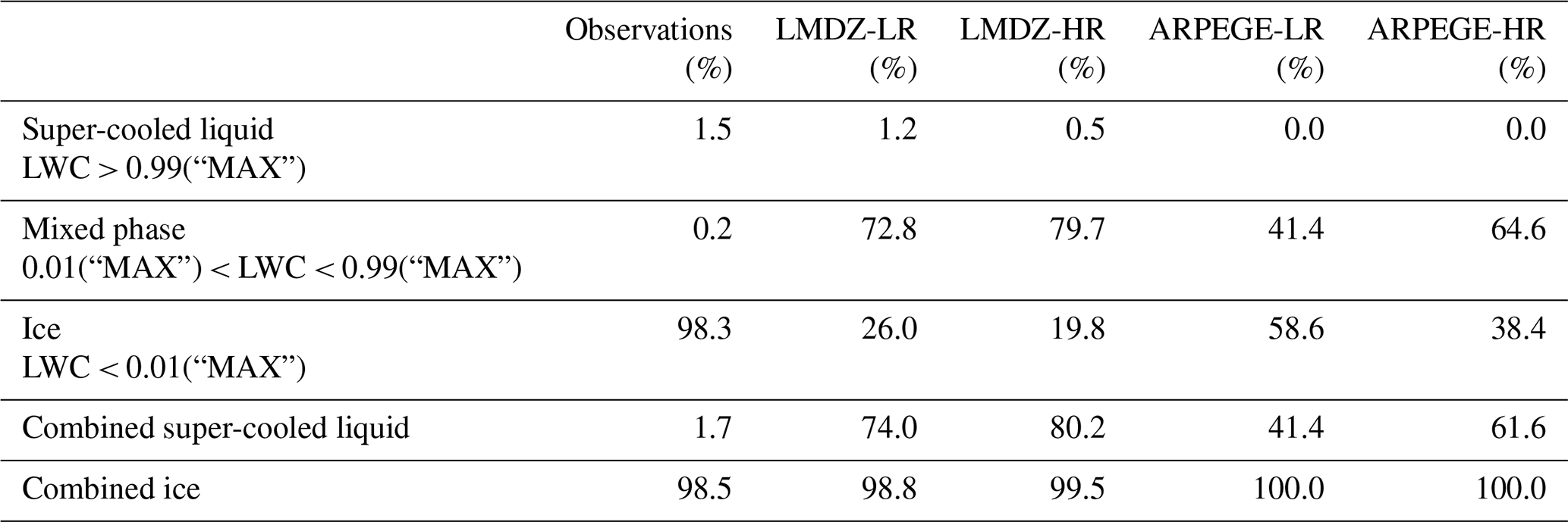
Given the change by the inclusion of LWC in the definition of the IWC, it is useful to know the proportion of ice, mixed-phase, and super-cooled liquid points that make up these distributions. We arbitrarily define ice points in the model to be those in which the LWC component of the “maximum” IWC is less than 1 % and “pure” super-cooled liquid to be points in which the LWC component is greater than 99 % of the “maximum” IWC; all other points are mixed phase. These results are compared with those points defined as super-cooled liquid, mixed phase, and ice retrieved IWC from RALI measurements. To ensure a fair comparison between ice and super-cooled liquid water, the “pure” values are combined with the mixed-phase values. Table 3 shows that whilst the combined ice points exceed those of the observations (particularly for ARPEGE) the values are not unreasonable. However, when the combined super-cooled liquid water is considered, the models significantly overestimate the amount of super-cooled liquid points by factors of 24–47. Considering Table 3 alongside the earlier discussion of the impact of adding LWC shows that the super-cooled liquid water being added to ARPEGE is of a smaller magnitude than that of LMDZ. It is also worth noting that although the LR hindcasts are more largely underestimating the IWC than the HR hindcasts, they are closer to the observations than the HR hindcasts in the percentage of super-cooled water.
Table 3The fraction of points within F7 that have values deemed as super-cooled liquid, mixed phase, and ice. “MAX” equals IWC plus LWC, combined super-cooled liquid equals super-cooled liquid plus mixed phase, and combined ice equals ice plus mixed phase. The hindcasts are initiated at 00:00 UTC 1 October 2016 and use the nearest grid point to the flight path from the two times surrounding the flight path (12:00 and 15:00 UTC 2 October 2016; T+36–39 h).
Radar reflectivities confirm the strong underestimation of IWC in the hindcasts (Fig. 12). The smaller values reached by LMDZ compared to ARPEGE are probably due to the larger percentage of liquid hydrometeors which induce smaller reflectivities than ice. It also confirms that the LR hindcasts outperform the HR hindcasts and ARPEGE is better than LMDZ in terms of shape of the IWC distribution. Despite a systematic underestimation of reflectivity at all levels, the ARPEGE-LR reflectivity exhibits the closest shape to the observations compared to the other three hindcasts.

Figure 12Contour frequency altitude diagrams (CFADs) of radar reflectivity for F7 (a) RASTA observations, (b) ARPEGE-LR, (c) ARPEGE-HR, (d) LMDZ-LR, and (e) LMDZ-HR. The hindcasts are initiated at 00:00 UTC 1 October 2016 and use the nearest grid point to the flight path from the two times surrounding the flight path (12:00 and 15:00 UTC 2 October 2016; T+36–39 h). The colour scale applies to all panels. No mask to the observations has been applied here.
Finally, to be confident in the above results, additional figures are presented in the Supplement. Figures S5 to S7 support the above findings by doing the same analysis along flight F6. Also, a comparison between RALI and CloudSat–CALIPSO measurements has been made along the common path of flight F7 and the A-train. The CloudSat reflectivities have a similar structure and similar amplitude to the RALI reflectivities (Fig. S8c, d). The DARDAR and RALI target classifications tend to agree with the main discrepancies originating from the time shift and the higher noise in CALIPSO backscatter and the lower sensitivity of RASTA close to the surface. This explains why the super-cooled layer detection is consistent, but the mixed-phase attribution is slightly different due to the radars sensitivity (Fig. S8e, f). Despite these differences regions of combined super-cooled liquid (super-cooled plus mixed phase) are rather similar, which gives confidence in the above conclusions.
To conclude, LMDZ produces more IWC which is associated with a more intense latent heating than ARPEGE. In that sense, it is closer to the observations. However, the ratio between liquid vs. solid species contributing to the IWC is less realistic in LMDZ than ARPEGE. Hence, it is worth noting that whilst the IWC can provide some information about the diabatic heating, caution is needed in interpreting the results as it does not provide complete information to be able to determine which of the two models produce the better heating compared to reality. However, the microphysical observations from flights during field campaigns are still useful in helping to identify the deficiencies of each model and determine what processes are linked in the models and why one of the models produces a more active cyclone compared to the other.
The representation of the Stalactite cyclone in the two atmospheric GCMs, ARPEGE-Climat 6.3 (hereafter ARPEGE) and LMDZ6A (hereafter LMDZ), corresponding to the atmospheric components of the CNRM and IPSL climate models (CNRM-CM6-1 and IPSL-CM6A) has been examined in detail. The two models are run at two resolutions: one at a coarse resolution of approximately 150–200 km (LR) and the other at a higher resolution of approximately 50 km (HR). The T-AMIP protocol is used to determine how well the climate models can represent the physical processes linked to the Stalactite cyclone and how well it compares to flight observations made during the NAWDEX field campaign. The protocol gives us valuable insight into the formation of the Stalactite cyclone.

Figure 13A schematic of the Stalactite cyclone. The mesoscale convective system (0) that initiates the diabatic Rossby vortex (1) that travels along the blue arrow. The northern precursor (2) with upper-level PV cut-off that moves towards the diabatic Rossby vortex and initiates a roll-up between the two precursors at cyclogenesis to create the Stalactite cyclone (3). Explosive deepening occurs as a result of strong diabatic heating throughout the column and the interaction with a series of embedded upper-level high-PV regions (the upper-level forcing here is depicted in the form of successive troughs in geopotential height moving in the direction of the white arrow; 4). Flight observations (5) indicate that ice water content is underestimated and so could have impacts on the diabatic heating and evolution of the cyclone.
Figure 13 shows a schematic of the many stages of the Stalactite cyclone: from initiation as a diabatic Rossby vortex (DRV) initiated from a mesoscale convective system (point 0) through the merger of the DRV (point 1) and a dynamical forcing factor (point 2) at cyclogenesis (point 3) to its rapid deepening (point 4) and comparisons with the observations (point 5) then around to cyclolysis. There are differences between each of the models and with the analysis at each of these points, and these are summarised in the main results below. The points are numbered based on the schematic (Fig. 13).
- 1.
All hindcasts produce a DRV to some degree of accuracy: LR hindcasts produce a qualitative DRV, whereas HR hindcasts produce a quantitative DRV that meets the criteria of Boettcher and Wernli (2013).
- 2.
All models produce an upper-level potential vorticity cut-off. However, due to its fine-scale structure, the cut-off is not as intense nor as deep in the LR hindcasts as in the HR hindcasts and analysis.
- 3.
Due to the above, the initial deepening associated with the vortex roll-up between the two precursors at cyclogenesis is weaker in LR hindcasts, and the initial deepening is better represented when the resolution increases. The reduced initial deepening implies that LR versions cannot fully (dynamically) represent the Stalactite cyclone. In particular, they do not represent the right tracks because their interaction with the upper-level PV reservoir is too late.
- 4a.
All hindcasts produce an explosively deepening cyclone with near 24 hPa deepening in 24 h during the mature stage similar to the analysis. However, the strong deepening stage is delayed by 24 h in LR hindcasts.
- 4b.
Diabatic heating extends throughout the troposphere during maximum deepening for both models but is larger in LMDZ compared to ARPEGE. Increasing the resolution does not increase the relative contribution of diabatic heating to the main deepening of the cyclone unlike in previous studies (e.g. Willison et al., 2013; Trzeciak et al., 2016). Instead, there are local increases in the diabatic heating which are particularly important for the northern precursor at cyclogenesis (Figs. 6 and S2).
- 5a.
Both models and resolutions underestimate the IWC from flight observations, even when super-cooled liquid water is taken into account, by a factor of 3–4 which is in agreement with Rysman et al. (2018). However, the shape of the vertical distribution of IWC is in good agreement for ARPEGE. The LMDZ hindcasts only come into agreement for the shape of the distribution with the observations when super-cooled liquid water is added to the ice. When all condensates are considered, the LMDZ model presents larger values compared to ARPEGE over the whole troposphere. This larger content of condensates is associated with larger diabatic heating and larger vertical velocities, and hence it provides an explanation for the larger deepening rate in LMDZ compared to ARPEGE.
- 5b.
Both models appear to substantially overestimate the amount of super-cooled liquid water content in the cyclone. This comes as a result of an increased number of mixed-phase grid points.
Thus, returning to the originally proposed questions and criteria for the correct representation of the Stalactite cyclone, the evidence suggests that climate models, when they are run at a coarse resolution, cannot represent the initial stage of the Stalactite cyclone, but they can produce the main deepening during the mature stage. The results also indicate that improvements in dynamical processes are as (if not more) important as improvements in diabatic processes with increasing resolution. The results further show that microphysical properties can be used, with caution, qualitatively to provide indirect information on the diabatic heating in climate models. Therefore, the flight observations provide (albeit not complete) an interesting insight into whether the climate models are producing the correct heating. This last topic is currently being investigated further by the authors with respect to the downstream impact of extratropical cyclones in climate models on subsequent ridge building.
Although the present results only apply for this particular case study3, the results have important implications and show areas that warrant further investigation. Firstly, it shows that the T-AMIP protocol is useful for considering the physical mechanisms that occur within cyclones and their interaction with dynamics. Secondly, it shows that increasing resolution does help with the representation of cyclones such that within the next few years, when climate models will be regularly run at ca. 50 km, many synoptic-scale features of the atmosphere will be dynamically well represented. Finally, and arguably most critically, it warns that although climate models may produce similar cyclones they can be doing so for very different reasons, and these reasons are likely to have an influence upon other areas of the climate system and the response of model cyclones to climate change. We recommend that further research occurs into the partition of super-cooled liquid water, mixed phase, and ice water in models (and the influence this has on cyclone representation) and that further comparisons with observations are made in all regions as this will have a strong influence on the development of microphysical schemes in climate and weather prediction models. Therefore, whilst signs are encouraging for future versions of climate models, caution is still needed when considering current simulations of future climate scenarios and the impact of extratropical cyclones, particularly for regional impact-based studies.
Data are available by contacting either David L. A. Flack at david.flack1@metoffice.gov.uk or the corresponding author.
The supplement related to this article is available online at: https://doi.org/10.5194/wcd-2-233-2021-supplement.
All authors contributed to the writing and editing of the paper, as well as the scientific discussions. DLAF produced the first draft and conducted the model analysis. IM performed the IPSL-CM6A simulations and RR the CNRM-CM6-1 simulations. GR and SB designed the study. JD, QC, and JP provided the observational datasets.
The authors declare that they have no conflict of interest.
This work is part of the DIP-NAWDEX (DIabatic Processes in the North Atlantic Waveguide and Downstream impact EXperiment) project which is supported and funded by the Agence Nationale de la Recherche (ANR). The authors wish to acknowledge the use of the Ferret programme for analysis and Figs. 1–9 and S1–S4 in this paper. Ferret is a product of NOAA's Pacific Marine Environmental Laboratory (information is available at http://ferret.pmel.noaa.gov/Ferret/, last access: 19 March 2021). We further acknowledge the use of imagery from the NASA Worldview application (https://worldview.earthdata.nasa.gov, last access: 19 March 2021), part of the NASA Earth Observing System Data and Information System (EOSDIS). We also wish to thank the two anonymous reviewers whose comments have helped improve the manuscript.
This research has been supported by the Agence Nationale de la Recherche (grant no. ANR-17-CE01-0010-01). The funding for Ionela Musat for running the LMDZ T-AMIP experiments was from the European Research Council (grant no. 694768). The LMDZ simulations were performed using the HPC from GENCI-IDRIS (grant no. 0292). The airborne measurements and the SAFIRE Falcon flights received direct funding from IPSL, Météo-France, INSU-LEFE, EUFAR-NEAREX, and ESA (EPATAN, contract no. 4000119015/16/NL/CT/gp).
This paper was edited by Martin Singh and reviewed by two anonymous referees.
Bengtsson, L., Hodges, K. I., and Keenlyside, N.: Will Extratropical Storms Intensify in a Warmer Climate?, J. Climate, 22, 2276–2301, https://doi.org/10.1175/2008JCLI2678.1, 2009. a
Blanchard, N., Pantillon, F., Chaboureau, J.-P., and Delanoë, J.: Organization of convective ascents in a warm conveyor belt, Weather Clim. Dynam., 1, 617–634, https://doi.org/10.5194/wcd-1-617-2020, 2020. a
Bodas-Salcedo, A., Webb, M. J., Bony, S., Chepfer, H., Dufresne, J.-L., Klein, S. A., Zhang, Y., Marchand, R., Haynes, J. M., Pincus, R., and John, V. O.: COSP: Satellite simulation software for model assessment, B. Am. Meteorol. Soc., 92, 1023–1043, https://doi.org/10.1175/2011BAMS2856.1, 2011. a
Boettcher, M. and Wernli, H.: A 10-yr Climatology of Diabatic Rossby Waves in the Northern Hemisphere, Mon. Weather Rev., 141, 1139–1154, https://doi.org/10.1175/MWR-D-12-00012.1, 2013. a, b, c, d, e, f
Bony, S., Bellon, G., Klocke, D., Sherwood, S., Fermepin, S., and Denvil, S.: Robust direct effect of carbon dioxide on tropical circulation and regional precipitation, Nat. Geosci., 6, 447–451, https://doi.org/10.1038/ngeo1799, 2013. a
Boucher O., Servonnat, J., Albright, A. L., et al.: Presentation and evaluation of the IPSL-CM6A-LR climate model, J. Adv. Model. Earth Sy., 12, e2019MS002010, https://doi.org/10.1029/2019MS002010, 2020. a
Brient, F., Roehrig, R., and Voldoire, A.: Evaluating Marine Stratocumulus Clouds in the CNRM-CM6-1 Model Using Short-Term Hindcasts, J. Atmos. Model Dev., 11, 127–148, https://doi.org/10.1029/2018MS001461, 2019. a, b
Catto, J. L., Shaffrey, L. C., and Hodges, K. I.: Can Climate Models Capture the Structure of Extratropical Cyclones?, J. Climate, 23, 1621–1635, https://doi.org/10.1175/2009JCLI3318.1, 2010. a
Catto, J. L., Shaffrey, L. C., and Hodges, K. I.: Northern Hemisphere Extratropical Cyclones in a Warming Climate in the HiGEM High-Resolution Climate Model, J. Climate, 24, 5336–5352, https://doi.org/10.1175/2011JCLI4181.1, 2011. a
Cazenave, Q., Ceccaldi, M., Delanoë, J., Pelon, J., Groß, S., and Heymsfield, A.: Evolution of DARDAR-CLOUD ice cloud retrievals: new parameters and impacts on the retrieved microphysical properties, Atmos. Meas. Tech., 12, 2819–2835, https://doi.org/10.5194/amt-12-2819-2019, 2019. a
Coronel, B., Ricard, D., Rivière, G., and Arbogast, P.: Role of moist processes in the tracks of idealized midlatitude surface cyclones, J. Atmos. Sci., 72, 2979–2996, 2015. a, b
Davis, C. A., Stoelinga, M. T., and Kuo, Y.-H.: The integrated effect of condensation in numerical simulations of extratropical cyclogenesis, Mon. Weather Rev., 121, 2309–2330, 1993. a
Delanoë, J., Protat, A., Jourdan, O., Pelon, J., Papazzoni, M., Dupuy, R., Gayet, J.-F., and Jouan, C.: Comparison of Airborne In Situ, Airborne Radar–Lidar, and Spaceborne Radar–Lidar Retrievals of Polar Ice Cloud Properties Sampled during the POLARCAT Campaign, J. Atmos. Ocean. Technol., 30, 57–73, https://doi.org/10.1175/JTECH-D-11-00200.1, 2013. a
Delanoë, J. and Hogan, R. J.: A variational scheme for retrieving ice cloud properties from combined radar, lidar, and infrared radiometer, J. Geophys. Res.-Atmos., 113, D07204, https://doi.org/10.1029/2007JD009000, 2008. a
Delanoë, J. and Hogan, R. J.: Combined CloudSat-CALIPSO-MODIS retrievals of the properties of ice clouds, J. Geophys. Res.-Atmos., 115, D00H29, https://doi.org/10.1029/2009JD012346, 2010. a
Eyring, V., Bony, S., Meehl, G. A., Senior, C. A., Stevens, B., Stouffer, R. J., and Taylor, K. E.: Overview of the Coupled Model Intercomparison Project Phase 6 (CMIP6) experimental design and organization, Geosci. Model Dev., 9, 1937–1958, https://doi.org/10.5194/gmd-9-1937-2016, 2016. a
Fermepin, S. and Bony, S.: Influence of low-cloud radiative effects on tropical circulation and precipitation, J. Atmos. Model Dev., 6, 513–526, https://doi.org/10.1002/2013MS000288, 2014. a, b, c
Fink, A. H., Pohle, S., Pinto, J. G., and Knippertz, P.: Diagnosing the influence of diabatic processes on the explosive deepening of extratropical cyclones, Geophys. Res. Lett., 39, L07803, https://doi.org/10.1029/2012GL051025, 2012. a
Finnis, J., Holland, M. M., Serreze, M. C., and Cassano, J. J.: Response of Northern Hemisphere extratropical cyclone activity and associated precipitation to climate change, as represented by the Community Climate System Model, J. Geophys. Res.-Biogeosci., 112, G04S42, https://doi.org/10.1029/2006JG000286, 2007. a
Fouquart, Y. and Bonnel, B.: Computations of solar heating of the Earth's atmosphere: A new parameterization, Beitr. Phys. Atmosph., 53, 35–61, 1980. a, b
Guérémy, J.: A continuous buoyancy based convection scheme: one-and three-dimensional validation, Tellus A, 63, 687–706, https://doi.org/10.1111/j.1600-0870.2011.00521.x, 2011. a
Harvey, B. J., Shaffrey, L. C., Woollings, T. J., Zappa, G., and Hodges, K. I.: How large are projected 21st century storm track changes?, Geophys. Res. Lett., 39, L18707, https://doi.org/10.1029/2012GL052873, 2012. a
Hawkins, E. and Sutton, R.: The Potential to Narrow Uncertainty in Regional Climate Predictions, B. Am. Meteorol. Soc., 90, 1095–1108, https://doi.org/10.1175/2009BAMS2607.1, 2009. a
Holton, J.: An Introduction to Dynamic Meteorology, 4th ed. International Geophysics Series, Vol. 88, Elsevier Academic Press, Burlington, Massachusetts, 535 pp., 2004. a
Hoskins, B. J. and Pedder, M. A.: The diagnosis of middle latitude synoptic development, Q. J. Roy. Meteor. Soc., 106, 707–719, https://doi.org/10.1002/qj.49710645004, 1980. a
Hoskins, B. J., Draghici, I., and Davies, H. C.: A new look at the ω-equation, Q. J. Roy. Meteor. Soc., 104, 31–38, https://doi.org/10.1002/qj.49710443903, 1978. a
Hourdin, F., Jam, A., Rio, C., Couvreux, F., Sandu, I., Lefebvre, M.-P., Brient, F., and Idelkadi, A.: Unified Parameterization of Convective Boundary Layer Transport and Clouds With the Thermal Plume Model, J. Atmos. Model Dev., 11, 2910–2933, https://doi.org/10.1029/2019MS001666, 2019. a
Hourdin, F., Rio, C., Grandpeix, J.-Y., Madeleine, J.-B., Cheruy, F., Rochetin, N., Jam, A., Musat, I., Idelkadi, A., Fairhead, L., Foujols, M.-A., Mellul, L., Traore, A.-K., Dufresne, J.-L., Boucher, O., Lefebvre, M.-P., Millour, E., Vignon, E., Jouhaud, J. F., Diallo, B., Lott, F., Gastineau, G., Caubel, A., Meurdesoif, Y., and Ghattas, J.: LMDZ6A: the atmospheric component of the IPSL climate model with improved and better tuned physics, J. Atmos. Model Dev., 12, e2019MS001892, https://doi.org/10.1029/2019MS001892, 2020. a
Karmalkar, A. V., Sexton, D. M. H., Murphy, J. M., Booth, B. B. B., Rostron, J. W., and McNeall, D. J.: Finding plausible and diverse variants of a climate model. Part II: development and validation of methodology, Clim. Dynam., 53, 847–877, https://doi.org/10.1007/s00382-019-04617-3, 2019. a
Klocke, D. and Rodwell, M. J.: A comparison of two numerical weather prediction methods for diagnosing fast-physics errors in climate models, Q. J. Roy. Meteor. Soc., 140, 517–524, https://doi.org/10.1002/qj.2172, 2014. a
Li, J., Chen, H., Rong, X., Su, J., Xin, Y., Furtado, K., Milton, S., and Li, N.: How Well Can a Climate Model Simulate an Extreme Precipitation Event: A Case Study Using the Transpose-AMIP Experiment, J. Climate, 31, 6543–6556, https://doi.org/10.1175/JCLI-D-17-0801.1, 2018. a
Lopez, P.: Implementation and validation of a new prognostic large-scale cloud and precipitation scheme for climate and data-assimilation purposes, Q. J. Roy. Meteor. Soc., 128, 229–257, https://doi.org/10.1256/00359000260498879, 2002. a
Ma, H.-Y., Xie, S., Boyle, J. S., Klein, S. A., and Zhang, Y.: Metrics and Diagnostics for Precipitation-Related Processes in Climate Model Short-Range Hindcasts, J. Climate, 26, 1516–1534, https://doi.org/10.1175/JCLI-D-12-00235.1, 2013. a, b
Ma, H.-Y., Xie, S., Klein, S. A., Williams, K. D., Boyle, J. S., Bony, S., Douville, H., Fermepin, S., Medeiros, B., Tyteca, S., Watanabe, M., and Williamson, D.: On the Correspondence between Mean Forecast Errors and Climate Errors in CMIP5 Models, J. Climate, 27, 1781–1798, https://doi.org/10.1175/JCLI-D-13-00474.1, 2014. a
Maddison, J. W., Gray, S. L., Martínez-Alvarado, O., and Williams, K. D.: Upstream Cyclone Influence on the Predictability of Block Onsets over the Euro-Atlantic Region, Mon. Weather Rev., 147, 1277–1296, https://doi.org/10.1175/MWR-D-18-0226.1, 2019. a, b
Maddison, J. W., Gray, S. L., Martínez-Alvarado, O., and Williams, K. D.: Impact of model upgrades on diabatic processes in extratropical cyclones and downstream forecast evolution, Q. J. Roy. Meteor. Soc., 146, 1322–1350, https://doi.org/10.1002/qj.3739, 2020. a
Madeleine, J.-B., Hourdin, F., Grandpeix, J.-P., Rio, C., Dufresne, J.-L., Vignon, E., Boucher, O., Konsta, D., Cheruy, F., Musat, I., Idelkadi, A., Fairhead, L., Millour, E., Lefebvre, M.-P., Mellul, L., Rochetin, N., Lemonnier, F., Touzé‐Peiffer, L., and Bonazzola, M.: Improvedrepresentation of clouds in theatmospheric component LMDZ6A ofthe IPSL-CM6A Earth system model, J. Adv. Model. Earth Sy., 12, e2020MS002046, https://doi.org/10.1029/2020MS002046, 2020. a
McDonald, R. E.: Understanding the impact of climate change on Northern Hemisphere extra-tropical cyclones, Clim. Dynam., 37, 1399–1425, https://doi.org/10.1007/s00382-010-0916-x, 2011. a
Mlawer, E. J., Taubman, S. J., Brown, P. D., Iacono, M. J., and Clough, S. A.: Radiative transfer for inhomogeneous atmospheres: RRTM, a validated correlated-k model for the longwave, J. Geophys. Res.-Atmos., 102, 16663–16682, https://doi.org/10.1029/97JD00237, 1997. a, b
Morcrette, J.-J., Barker, H. W., Cole, J. N. S., Iacono, M. J., and Pincus, R.: Impact of a New Radiation Package, McRad, in the ECMWF Integrated Forecasting System, Mon. Weather Rev., 136, 4773–4798, https://doi.org/10.1175/2008MWR2363.1, 2008. a
Oertel, A., Boettcher, M., Joos, H., Sprenger, M., Konow, H., Hagen, M., and Wernli, H.: Convective activity in an extratropical cyclone and its warm conveyor belt – a case-study combining observations and a convection-permitting model simulation, Q. J. Roy. Meteor. Soc., 145, 1406–1426, https://doi.org/10.1002/qj.3500, 2019. a
Orlanski, I. and Katzfey, J.: The Life Cycle of a Cyclone Wave in the Southern Hemisphere. Part I: Eddy Energy Budget, J. Atmos. Sci., 48, 1972–1998, https://doi.org/10.1175/1520-0469(1991)048<1972:TLCOAC>2.0.CO;2, 1991. a
Oruba, L., Lapeyre, G., and Rivière, G.: On the Poleward Motion of Midlatitude Cyclones in a Baroclinic Meandering Jet, J. Atmos. Sci., 70, 2629–2649, 2013. a
Pearson, K. J., Shaffrey, L. C., Methven, J., and Hodges, K. I.: Can a climate model reproduce extreme regional precipitation events over England and Wales?, Q. J. Roy. Meteor. Soc., 141, 1466–1472, https://doi.org/10.1002/qj.2428, 2015. a
Petterssen, S. and Smebye, S. J.: On the development of extratropical cyclones, Q. J. Roy. Meteor. Soc., 97, 457–482, 1971. a
Phillips, T. J., Potter, G. L., Williamson, D. L., Cederwall, R. T., Boyle, J. S., Fiorino, M., Hnilo, J. J., Olson, J. G., Xie, S., and Yio, J. J.: Evaluating Parameterizations in General Circulation Models: Climate Simulation Meets Weather Prediction, B. Am. Meteor. Soc., 85, 1903–1916, https://doi.org/10.1175/BAMS-85-12-1903, 2004. a
Piriou, J.-M., Redelsperger, J.-L., Geleyn, J.-F., Lafore, J.-P., and Guichard, F.: An Approach for Convective Parameterization with Memory: Separating Microphysics and Transport in Grid-Scale Equations, J. Atmos. Sci., 64, 4127–4139, https://doi.org/10.1175/2007JAS2144.1, 2007. a
Rivière, G. and Joly, A.: Role of the Low-Frequency Deformation Field on the Explosive Growth of Extratropical Cyclones at the Jet Exit. Part II: Baroclinic Critical Region, J. Atmos. Sci., 63, 1982–1995, https://doi.org/10.1175/JAS3729.1, 2006. a, b
Rivière, G., Arbogast, P., Lapeyre, G., and Maynard, K.: A potential vorticity perspective on the motion of a mid-latitude winter storm, Geophys. Res. Lett., 39, L12808, https://doi.org/10.1029/2012GL052440, 2012. a
Rivière, G., Arbogast, P., and Joly, A.: Eddy kinetic energy redistribution within windstorms Klaus and Friedhelm, Q. J. Roy. Meteor. Soc., 141, 925–938, 2015. a
Rochetin, N., Grandpeix, J.-Y., Rio, C., and Couvreux, F.: Deep Convection Triggering by Boundary Layer Thermals. Part II: Stochastic Triggering Parameterization for the LMDZ GCM, J. Atmos. Sci., 71, 515–538, https://doi.org/10.1175/JAS-D-12-0337.1, 2014. a
Roehrig, R., Beau, I., Saint-Martin, D., Alias, A., Decharme, B., Guérémy, J.-F., Voldoire, A., Ahmat Younous, A.-L., Bazile, E., Belamari, S., Blein, S., Bouniol, D., Bouteloup, Y., Cattiaux, J., Chauvin, F., Chevallier, M., Colin, J., Douville, H., Marquet, P., Michou, M., Nabat, P., Oudar, T., Peyrillé, P., Piriou, J.-M., Salas y Melia, D., Séférian, R., and Sénési, S.: The CNRM global atmosphere model ARPEGE-Climat 6.3: description and evaluation, J. Atmos. Model Dev., 12, e2020MS002075, https://doi.org/10.1029/2020MS002075, 2020. a
Rysman, J.-F., Berthou, S., Claud, C., Drobinski, P., Chaboureau, J.-P., and Delanoë, J.: Potential of microwave observations for the evaluation of rainfall and convection in a regional climate model in the frame of HyMeX and MED-CORDEX, Clim. Dynam., 51, 837–855, https://doi.org/10.1007/s00382-016-3203-7, 2018. a, b
Sanders, F. and Gyakum, J. R.: Synoptic-Dynamic Climatology of the “Bomb”, Mon. Weather Rev., 108, 1589–1606, https://doi.org/10.1175/1520-0493(1980)108<1589:SDCOT>2.0.CO;2, 1980. a
Schäfler, A., Craig, G., Wernli, H., Arbogast, P., Doyle, J. D., McTaggart-Cowan, R., Methven, J., Rivière, G., Ament, F., Boettcher, M., Bramberger, M., Cazenave, Q., Cotton, R., Crewell, S., Delanoë, J., Dörnbrack, A., Ehrlich, A., Ewald, F., Fix, A., Grams, C. M., Gray, S. L., Grob, H., Groß, S., Hagen, M., Harvey, B., Hirsch, L., Jacob, M., Kölling, T., Konow, H., Lemmerz, C., Lux, O., Magnusson, L., Mayer, B., Mech, M., Moore, R., Pelon, J., Quinting, J., Rahm, S., Rapp, M., Rautenhaus, M., Reitebuch, O., Reynolds, C. A., Sodemann, H., Spengler, T., Vaughan, G., Wendisch, M., Wirth, M., Witschas, B., Wolf, K., and Zinner, T.: The North Atlantic Waveguide and Downstream Impact Experiment, B. Am. Meteor. Soc., 99, 1607–1637, https://doi.org/10.1175/BAMS-D-17-0003.1, 2018. a, b, c, d, e, f, g
Seiler, C. and Zwiers, F. W.: How well do CMIP5 climate models reproduce explosive cyclones in the extratropics of the Northern Hemisphere?, Clim. Dynam., 46, 1241–1256, https://doi.org/10.1007/s00382-015-2642-x, 2016. a, b
Sexton, D. M. H., Karmalkar, A. V., Murphy, J. M., Williams, K. D., Boutle, I. A., Morcrette, C. J., Stirling, A. J., and Vosper, S. B.: Finding plausible and diverse variants of a climate model. Part I: establishing the relationship between errors at weather and climate time scales, Clim. Dynam., 53, 989–1022, https://doi.org/10.1007/s00382-019-04625-3, 2019. a
Sinclair, V. A., Rantanen, M., Haapanala, P., Räisänen, J., and Järvinen, H.: The characteristics and structure of extra-tropical cyclones in a warmer climate, Weather Clim. Dynam., 1, 1–25, https://doi.org/10.5194/wcd-1-1-2020, 2020. a, b, c, d
Trzeciak, T. M., Knippertz, P., Pirret, J. S. R., and Williams, K. D.: Can we trust climate models to realistically represent severe European windstorms?, Clim. Dynam., 46, 3431–3451, https://doi.org/10.1007/s00382-015-2777-9, 2016. a, b, c, d, e, f
Voldoire, A., Saint-Martin, D., Sénési, S., Decharme, B., Alias, A., Chevallier, M., Colin, J., Guérémy, J.-F., Michou, M., Moine, M.-P., Nabat, P., Roehrig, R., Salas y Mélia, D., Séférian, R., Valcke, S., Beau, I., Belamari, S., Berthet, S., Cassou, C., Cattiaux, J., Deshayes, J., Douville, H., Ethé, C., Franchistéguy, L., Geoffroy, O., Lévy, C., Madec, G., Meurdesoif, Y., Msadek, R., Ribes, A., Sanchez-Gomez, E., Terray, L., and Waldman, R.: Evaluation of CMIP6 DECK Experiments With CNRM-CM6-1, J. Atmos. Model Dev., 11, 2177–2213, https://doi.org/10.1029/2019MS001683, 2019. a
Wan, H., Rasch, P. J., Zhang, K., Qian, Y., Yan, H., and Zhao, C.: Short ensembles: an efficient method for discerning climate-relevant sensitivities in atmospheric general circulation models, Geosci. Model Dev., 7, 1961–1977, https://doi.org/10.5194/gmd-7-1961-2014, 2014. a
Williams, K. D., Bodas-Salcedo, A., Déqué, M., Fermepin, S., Medeiros, B., Watanabe, M., Jakob, C., Klein, S. A., Senior, C. A., and Williamson, D. L.: The Transpose-AMIP II Experiment and Its Application to the Understanding of Southern Ocean Cloud Biases in Climate Models, J. Climate, 26, 3258–3274, https://doi.org/10.1175/JCLI-D-12-00429.1, 2013. a, b, c, d
Willison, J., Robinson, W. A., and Lackmann, G. M.: The Importance of Resolving Mesoscale Latent Heating in the North Atlantic Storm Track, J. Atmos. Sci., 70, 2234–2250, https://doi.org/10.1175/JAS-D-12-0226.1, 2013. a, b, c, d
Zappa, G., Shaffrey, L. C., and Hodges, K. I.: The Ability of CMIP5 Models to Simulate North Atlantic Extratropical Cyclones, J. Climate, 26, 5379–5396, https://doi.org/10.1175/JCLI-D-12-00501.1, 2013a. a
Zappa, G., Shaffrey, L. C., Hodges, K. I., Sansom, P. G., and Stephenson, D. B.: A Multimodel Assessment of Future Projections of North Atlantic and European Extratropical Cyclones in the CMIP5 Climate Models, J. Climate, 26, 5846–5862, https://doi.org/10.1175/JCLI-D-12-00573.1, 2013b. a, b
In essence, this is the same phenomenon as a diabatic Rossby wave (see Appendix of Boettcher and Wernli, 2013).
A deepening rate of 1 hPa h−1 for 24 h multiplied by sin(ϕ)sin(60) to adjust to the appropriate latitude to make it equivalent to at least 1 bergeron, where ϕ is the latitude.
A second cyclone (the following cyclone; IOP 7 of NAWDEX) related to the future work shows the same results (not shown).