Atmospheric convergence zones stemming from large-scale mixing

Organised cloud bands are important features of tropical and subtropical rainfall. These structures are often regarded as convergence zones, alluding to an association with coherent atmospheric flow. However, the flow kinematics is not usually taken into account in classification methods for this type of event, as large-scale lines are rarely evident in instantaneous diagnostics such as Eulerian convergence. Instead, existing convergence zone definitions rely on heuristic rules of shape, duration and size of cloudiness fields. Here we investigate the role of large-scale turbulence in shaping atmospheric moisture in South America. We employ the finite-time Lyapunov exponent (FTLE), a metric of deformation among neighbouring trajectories, to define convergence zones as attracting Lagrangian coherent structures (LCSs). Attracting LCSs frequent tropical and subtropical South America, with climatologies consistent with the South Atlantic Convergence Zone (SACZ), the South American Low-Level Jet (SALLJ) and the Intertropical Convergence Zone (ITCZ). In regions under the direct influence of the ITCZ and the SACZ, rainfall is significantly positively correlated with large-scale mixing measured by the FTLE. Attracting LCSs in south and southeast Brazil are associated with significant positive rainfall and moisture flux anomalies. Geopotential height composites suggest that the occurrence of attracting LCSs in these regions is related with teleconnection mechanisms such as the Pacific–South Atlantic. We believe that this kinematical approach can be used as an alternative to region-specific convergence zone classification algorithms; it may help advance the understanding of underlying mechanisms of tropical and subtropical rain bands and their role in the hydrological cycle.

1 Introduction

Large-scale organised zones of cloudiness and rainfall stand out in tropical and subtropical weather, which is otherwise dominated by non-organised convection. These cloud bands were initially identified in the equatorial belt (Alpert, 1945) and associated with the interaction of inter-hemispheric air masses along the easterlies (Fletcher, 1945; Simpson, 1947), i.e. the Intertropical Convergence Zone (ITCZ). Despite these historical associations with coherent trajectories, convergence zones have been more frequently identified by heuristic rules applied to satellite imagery or cloudiness/rainfall data (Barros et al., 2000; Van Der Wiel et al., 2015; Ambrizzi and Ferraz, 2015; Vindel et al., 2020). These approaches require detailed previous knowledge of the spatio-temporal characteristics of convergence zones in specific locations. Therefore, they do not provide a general definition for these events.

In other studies, convergence zones were characterised using the divergence of instantaneous or average velocity fields (Berry and Reeder, 2014; Weller et al., 2017). These approaches are in principle more general. However, because Eulerian metrics such as divergence reveal instantaneous features in their immediate neighbourhoods, they respond strongly to local processes such as convection. More generally, in unsteady flows, Eulerian features do not reveal the underlying structures of tracer mixing such as air mass interfaces (Boffetta et al., 2001; d'Ovidio et al., 2009). Rather, from the kinematics point of view, flow structures shaping tracer evolution are more suitably inspected under Lagrangian frameworks (Ottino, 1989; Pierrehumbert, 1991; Bowman, 2000; Haller and Yuan, 2000). By offering temporally integrated trajectory information, Lagrangian diagnostics synthesise pathline features that determine atmospheric transport.

In this study, we investigate attracting coherent structures arising from large-scale mixing in South America and their relationship with rainfall and water vapour. We propose that such structures are skeletons of atmospheric convergence zones and provide an identification criterion that can be applied to reanalyses and model data (Sects. 2 and 3). In Sect. 4, we discuss the physical interpretation of the quantities involved. In Sect. 5, we discuss the methodology applied to a recent South Atlantic Convergence Zone (SACZ) event. Finally, we present their impacts on rainfall and moisture fluxes in South America (Sect. 6) and associate them with teleconnections (Sect. 7).

1.1 Mixing and Lagrangian coherent structures in the atmosphere

In time-dependent flows, advection reshapes the distribution of tracers into complex filamentous patterns (Aref, 1984). This process of mixing intensifies tracer gradients and is characterised by the stretching and folding of parcels (Ottino, 1989); it can be observed in the atmosphere on synoptic timescales even in relatively simple flows (Welander, 1955). We consider convergence zones, from the point of view of mixing, as coherent structures associated with strong attraction of trajectories with the potential to organise moisture filaments or bands.

The finite-time Lyapunov exponent (FTLE) is a convenient tool to visualise underlying structures of flow mixing. It is defined as the average separation rate among neighbouring trajectories in a fixed propagation time interval. Ridges of the FTLE identify Lagrangian coherent structures (LCSs) (Haller, 2001; Shadden et al., 2005), structures by which advected passive tracer is strongly attracted or repelled within the time interval of interest. While this is an active area of research and more rigorous methods to investigate Lagrangian coherence exist (Haller and Beron-Vera, 2012; Farazmand et al., 2014), the FTLE has been employed in previous studies to investigate features of atmospheric and oceanic transport.

Pioneering studies by Pierrehumbert (1991) and Pierrehumbert and Yang (1993) applied the FTLE to investigate large-scale atmospheric mixing and tropics–extratropics transport barriers. Shepherd et al. (2000) computed probability density functions of the FTLE to investigate chaotic advection in the stratosphere. Rutherford et al. (2011) and Guo et al. (2016) employed the FTLE to visualise flow features in tropical cyclones. Garaboa-Paz et al. (2015, 2017) suggested that FTLE ridges are closely linked to atmospheric rivers in boreal winter, when advection shapes the spatial distribution of water vapour. The criterion for convergence zones proposed here is closely related to the framework proposed by Garaboa-Paz et al. (2015) for atmospheric rivers. We leverage the framework of LCSs to investigate the underlying flow features organising rainfall and moisture accumulation in South America.

1.2 Aspects of the moisture transport in South America

The largest portion of the South American continent is located in tropical and subtropical latitudes (Fig. 1). Along the western coast, the Andes mountain range extends across a considerable latitudinal interval as the dominant topographical feature. Its high altitudes pose a barrier to low and mid-tropospheric zonal flow. This barrier to the zonal flow deflects the climatological sea-to-land easterly flow as it enters the continent from the equatorial Atlantic, forming a meridional channel of north-to-south moisture transport between 850 and 700 hPa (Gimeno et al., 2016) that supplies moisture for rainfall in populated areas in southeastern and southern South America (Zemp et al., 2014). When intensified, this north-to-south moisture flux characterises the South American Low-Level Jet (SALLJ, Vera et al., 2006). Occasionally, the SALLJ resembles atmospheric rivers (Arraut et al., 2012; Poveda et al., 2014), filaments of intense moisture associated with the motion of extratropical cyclones (Dacre et al., 2015).

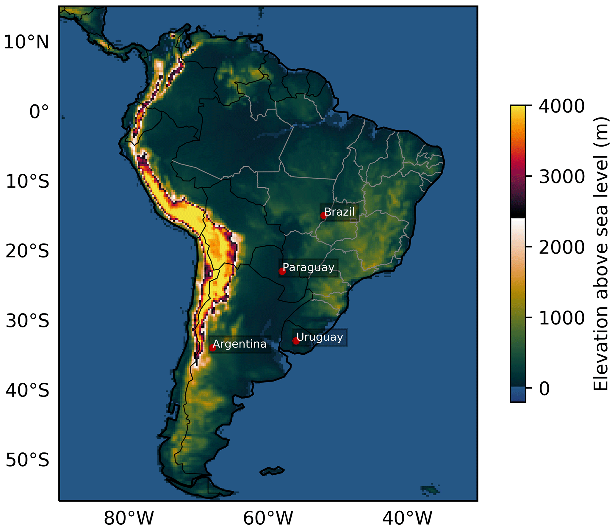
Figure 1 Elevation above the sea level. Derived from ECMWF's ERA5 surface geopotential.

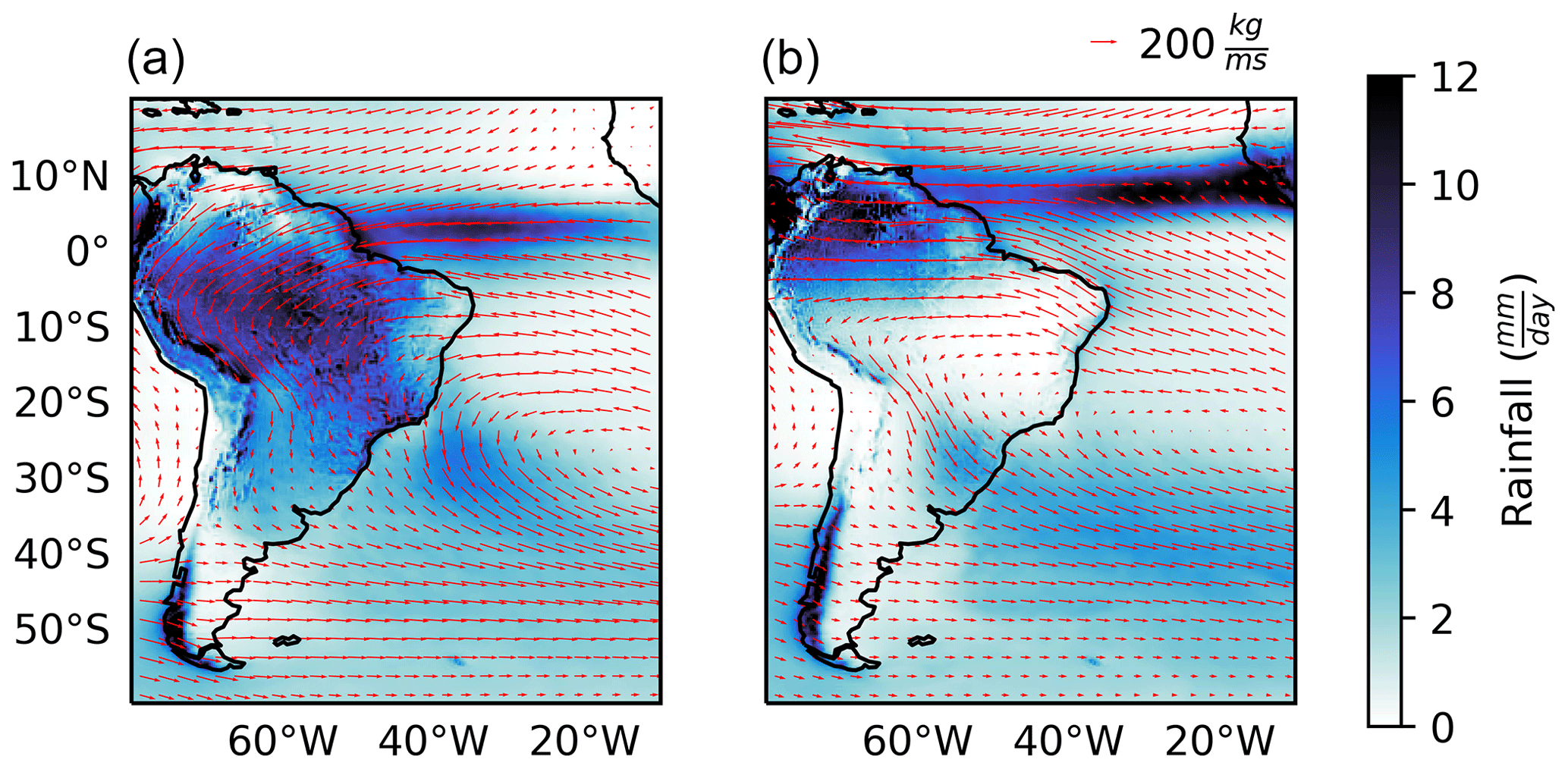
Figure 2 Mean rainfall and vertically integrated moisture flux (vectors) in DJF (a) and JJA (b). Averages were computed from ECMWF's ERA5 from 1980 to 2009.

During austral summer, increased sensible heat flux from the land surface and latent heat released through Amazonian convection, combined with the southward seasonal shift of the ITCZ, intensify the sea-to-land moisture transport, characterising the wet phase of the South American Monsoon System (SAMS, Marengo et al., 2012). The SAMS can be illustrated by the contrast between rainfall and moisture flux climatologies in summer and winter (Fig. 2). In summer, there is increased oceanic moist air input to the continent, associated with the tropical Atlantic easterlies and the South Atlantic subtropical high. The northeasterly moisture flux is deflected southeast after crossing the Amazon, supplying moisture for southeastern and southern South America (Zemp et al., 2014). This higher moisture input in summer coincides with higher rainfall, particularly in central and southeast Brazil. In winter, the angle of the easterlies in the Atlantic tilts northwards and the moisture flux from the South Atlantic subtropical high weakens, such that the moisture flux and rainfall are stronger in northernmost South America and weaker in most other parts of the continent. These observations point to the sensitivity of rainfall in central and southern South America to disruptions in the climatological SAMS moisture transport.

Extratropical cyclones are central to the synoptic-scale variability of the South American climate. These structures originate most frequently in cyclogenesis regions spanning from south Argentina to the coast of southeast Brazil (Crespo et al., 2020). These cyclones have an average life cycle of 3 d (Mendes et al., 2010); their associated cold fronts cause cold incursions (Lanfredi and De Camargo, 2018) and rainfall over the continent (Lenters and Cook, 1999; Vera et al., 2002). In the wet season of the SAMS, the interaction between tropical sources of heat and moisture with extratropical cyclones resonates at sub-monthly scales often manifested as diagonally oriented (northwest–southeast) cloud bands (Nieto and Chao, 2013; Raupp and Silva Dias, 2010). The diagonal aspect of these cloud bands is a characteristic feature of the SACZ; it has been attributed to the deformation of low-level vorticity centres by equatorward Rossby waves originating from circulation anomalies in the Pacific (Van Der Wiel et al., 2015). This relationship renders circulation and rainfall in the SACZ region sensitive to the Pacific–South American (PSA) teleconnection patterns (Mo and Paegle, 2001).

The objective definition and automatic identification of large-scale features shaping the moisture distribution in a long-term climatology is, thus, key to understanding the processes driving the seasonal and intraseasonal variability of the South American hydrological cycle. Currently, most identification algorithms for convergence zones focus on the SACZ and rely on rules of shape, duration and intensity of cloud bands usually given by an empirical orthogonal function (EOF) analysis of outgoing longwave radiation or rainfall (Barros et al., 2000; Jorgetti et al., 2014; Van Der Wiel et al., 2015; Ambrizzi and Ferraz, 2015). A drawback of cloudiness-based approaches is that they lack the means for attributing contributions from processes at different scales to a single cloud band. For example, cloudiness originating from local convection adjacent to cloudiness originating from large-scale flow coherence would appear to be the same structure from a satellite image. Furthermore, describing a physical phenomenon with a single EOF is problematic, as EOFs do not necessarily individually correspond to dynamical modes and can produce patterns with little connection to physical processes (Dommenget and Latif, 2002; Monahan et al., 2009; Fulton and Hegerl, 2019).

2 Mathematical framework

2.1 Vertically scaled horizontal moisture flux

Water vapour in the atmosphere concentrates close to its source at the Earth's surface. Thus, it is natural to analyse features of moisture transport using the low-level flow. Weller et al. (2017) employed an Eulerian metric to identify convergence lines at 950 hPa over the Pacific Ocean and Australian landmass. Garaboa-Paz et al. (2017) investigated atmospheric rivers at 850 hPa. While water vapour is concentrated at lower levels, selecting a particular level becomes problematic near topography, such as the Andes, for two reasons: (a) topography often crosses lower tropospheric pressure levels, and (b) it causes the level of maximum moisture transport to rise in its vicinity (Insel et al., 2010). The SALLJ, for example, transports substantial amounts of water vapour and flows parallel to the Andes between 850 and 700 hPa (Gimeno et al., 2016).

We employed a horizontal flow ${\mathit{V}}_{{\mathit{\rho }}_{\mathrm{v}}}$ derived from a vertical scaling of the horizontal momentum V_H that takes into account the vertical distribution of water vapour density (ρ_v). The scaling divides the vertically integrated moisture flux by the total column water vapour (Eq. 1). Physically, ${\mathit{V}}_{{\mathit{\rho }}_{\mathrm{v}}}$ is the average flow by which the total column water vapour is transported. A similar weighting was employed by Garaboa-Paz et al. (2015) to identify atmospheric rivers and by Ruiz-Vasquez et al. (2020) to investigate sources and sinks of water vapour in South America. It is important to notice, however, that strong vertical shear across heights of high moisture concentration may render ${\mathit{V}}_{{\mathit{\rho }}_{\mathrm{v}}}$ not representative of the actual horizontal pathways of moisture, obscuring the interpretation of attracting structures in this flow.

$$\begin{array}{}\text{(1)}& {\mathit{V}}_{{\mathit{\rho }}_{\mathrm{v}}}={\displaystyle \frac{\underset{\mathrm{0}}{\overset{\mathrm{\infty }}{\int }}{\mathit{\rho }}_{\mathrm{v}}{\mathit{V}}_{\mathrm{H}}\mathrm{d}z}{\underset{\mathrm{0}}{\overset{\mathrm{\infty }}{\int }}{\mathit{\rho }}_{\mathrm{v}}\mathrm{d}z}}\left[\mathrm{m}{\mathrm{s}}^{-\mathrm{1}}\right]\end{array}$$

We expect $V_{{\mathit{\rho }}_{\mathrm{v}}}$ not to be affected by moisture sources and sinks as the water vapour density ρ_v is both in the numerator and denominator of Eq. (1). In other words, the resulting flow is independent of the horizontal water vapour distribution. The role of ρ_v in Eq. (1) is, thus, only to provide a vertical weighting to V_H such that moist levels are favoured. The following sections discuss how we computed the trajectory deformation and identified LCSs in $V_{{\mathit{\rho }}_{\mathrm{v}}}$.

2.2 Finite-time Lyapunov exponent

The FTLE measures the average deformation rate among initially close trajectories after a characteristic advection time $\mathrm{\Delta }t=t_{\mathrm{1}}-t_{\mathrm{0}}$, where t₁ and t₀ are respectively the times of arrival and departure of these trajectories. The flow map $F_{t_{\mathrm{0}}}^{t_{\mathrm{1}}}$ (Eq. 2) links the departure position x₀(t₀) of a parcel to its arrival position ${\mathit{x}}_{\mathrm{1}}(t_{\mathrm{1}};{\mathit{x}}_{\mathrm{0}},t_{\mathrm{0}})$, where x₀ and x₁ are in IR² representing positions on the Earth's surface (latitude and longitude points).

$$\begin{array}{}\text{(2)}& F_{t_{\mathrm{0}}}^{t_{\mathrm{1}}}\left({\mathit{x}}_{\mathrm{0}}\right):={\mathit{x}}_{\mathrm{1}}\left(t_{\mathrm{1}};{\mathit{x}}_{\mathrm{0}},t_{\mathrm{0}}\right)\end{array}$$

The flow map can be found at any given point in time and space by numerically integrating the trajectories for every departure point on a discrete grid:

$$\begin{array}{}\text{(3)}& {\displaystyle \frac{D\mathit{x}}{\mathrm{D}t}}={\mathit{V}}_{{\mathit{\rho }}_{\mathrm{v}}}(\mathit{x},t).\end{array}$$

The exponential rate of separation of trajectories departing from the neighbourhood of x₀ is expressed by the FTLE, represented by σ:

$$\begin{array}{}\text{(4)}& \mathit{\sigma }\left({\mathit{x}}_{\mathrm{0}}\right)={\displaystyle \frac{\mathrm{1}}{\left|\mathrm{\Delta }t\right|}}\ln \left(\sqrt{{\mathit{\lambda }}_{\max }\left(C\right)}\right),\end{array}$$

where λ_max(C) is most positive eigenvalue of the right-hand Cauchy–Green strain tensor (Eq. 5).

$$\begin{array}{}\text{(5)}& C={\left[\mathrm{\nabla }{F}_{t_{\mathrm{0}}}^t\right]}^T\mathrm{\nabla }{F}_{t_{\mathrm{0}}}^t\end{array}$$

The gradient of the flow map $\mathrm{\nabla }{F}_{t_{\mathrm{0}}}^t$ was obtained by a centred finite-difference scheme (Haller, 2001) by converting x₀ and x₁ from spherical to Cartesian coordinates in IR³. Higher-accuracy discretisations can be obtained by solving Eq. (3) on unstructured meshes with adaptive resolution (Lekien and Ross, 2010). A more detailed derivation of the FTLE and the Cauchy–Green strain tensor can be found in Haller (2015) and references therein.

The eigenvalue λ_max(C) in Eq. (4) essentially quantifies the stretching or folding along the main axis of deformation experienced by a parcel undergoing transformation by the flow map. If the time trajectories are propagated backwards (i.e. back trajectories), the FTLE represents the exponential rate of folding; its ridges characterise attracting LCSs. In the forward-in-time case, the FTLE represents the stretching rate, and its ridges identify repelling LCSs. As we are interested in the Lagrangian skeletons that potentially organise moisture accumulation and rainfall along a preferred axis, we employ the backwards-in-time convention to identify attracting LCSs as FTLE ridges.

Here we employ an integration time interval of Δt=2 d, such that the trajectories are allowed to explore large-scale flow structures. This timescale is also not too long such that the effect of the typical extratropical cyclone, whose average life cycle is 3 d (Mendes et al., 2010), is filtered out. Although not shown here, features associated with the ITCZ and the SACZ were also found with other integration times (1, 3 and 4 d).

2.3 Convergence zones as FTLE ridges

While the scalar FTLE field at a given time characterises chaotic mixing spatially, its ridges are associated with the most locally intense attraction of back trajectories arriving in its neighbourhood (Haller, 2001; Allshouse and Peacock, 2015). Here we simply define attracting LCSs as curvature ridges of the FTLE scalar field (Shadden et al., 2005). We also impose additional criteria of size and intensity (see Sect. 3) to further isolate strong attracting structures that are more likely to organise large-scale cloud bands.

Shadden et al. (2005) argue that the flux across curvature FTLE ridges is negligible. This would mean that LCSs defined as such could be regarded as transport barriers. While this is not always true and counterexamples exist (Haller, 2011), FTLE can approximate transport barriers in geophysical flows such as stratospheric circulations (Boffetta et al., 2001), oceanic currents in the Gulf of Mexico (Olascoaga et al., 2006), and subtropical and polar jets (Beron-Vera et al., 2012). Moisture flux anomalies in Sect. 5 indicate that FTLE ridges in southeast Brazil act as barriers to important preferential pathways of moisture along the Andes, leading to negative rainfall anomalies in south Brazil and surroundings.

Therefore, by approximating transport barriers, our definition of convergence zone as attracting LCSs is also consistent with the association of convergence zones to air mass interfaces (Simpson, 1947). Such interfaces can be characterised as sharp gradients of the flow map that are directly represented in the scalar FTLE field.

3 Data and implementation

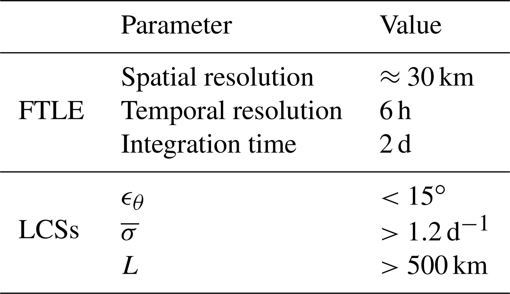
We computed ${\mathit{V}}_{{\mathit{\rho }}_{\mathrm{v}}}$ (Eq. 1) using total column water vapour and the zonal and meridional components of the vertically integrated moisture flux at full spatial resolution (≈30 km) and 6-hourly time resolution from the ECMWF's ERA5 reanalysis between 1980 and 2009. Gridded rainfall data are also obtained from ERA5 at the same spatial and temporal resolutions.

The back trajectories are calculated by numerically solving Eq. (3) with a stable extrapolating two-time-level Lagrangian advection scheme (SETTLS, Hortal, 2002), extrapolated in time iteratively using a second-order Taylor expansion. The velocity ${\mathit{V}}_{{\mathit{\rho }}_{\mathrm{v}}}$ along the trajectories was interpolated with a bivariate spherical spline (Dierckx, 1995). The intensity of the FTLE ridges is dependent on the accuracy of the advection scheme because numerical diffusion can weaken the gradients of the flow map. The trajectory integration domain was chosen as a wide area (85^∘ S/60^∘ N, 180^∘ W/30^∘ E) around South America in order to avoid boundary contamination in the domain of interest.

We identified candidate convergence zones as ridges of the FTLE scalar field by relaxing the criteria proposed by Shadden et al. (2005). The criteria involve isolating curves parallel to the FTLE gradient (condition SR1) and normal to the direction of most negative curvature of the FTLE scalar field (condition SR2). The latter is given by the eigendecomposition of the Hessian matrix. However, in practice, Shadden's criterion is too restrictive (Peikert et al., 2013). Peikert and Sadlo (2008) suggest relaxing SR1 by admitting a tolerance angle (ϵ_θ) between the curve representing the ridge and the gradient. We tested a range of ϵ_θ values and visually inspected the outputs to find that a tolerance angle of ϵ_θ=15^∘ produced satisfactory results. The derivatives for the gradient and the Hessian matrix were computed with a centred-difference scheme on the sphere.

Convergence zones were obtained by subsetting the candidate FTLE ridges by size and average intensity. Ridges with average FTLE ($\stackrel{\mathrm{‾}}{\mathit{\sigma }}$) below 1.2 d⁻¹ and major axis length (L) shorter than 500 km were discarded. While these thresholds are arbitrarily defined to filter out weaker and shorter structures, the relative distribution of convergence zones is robust to slight perturbations of the order of ±20 %. The steps to compute the FTLE and identify attracting LCSs are summarised in Fig. 3, and the relevant parameters are listed in Table 1.

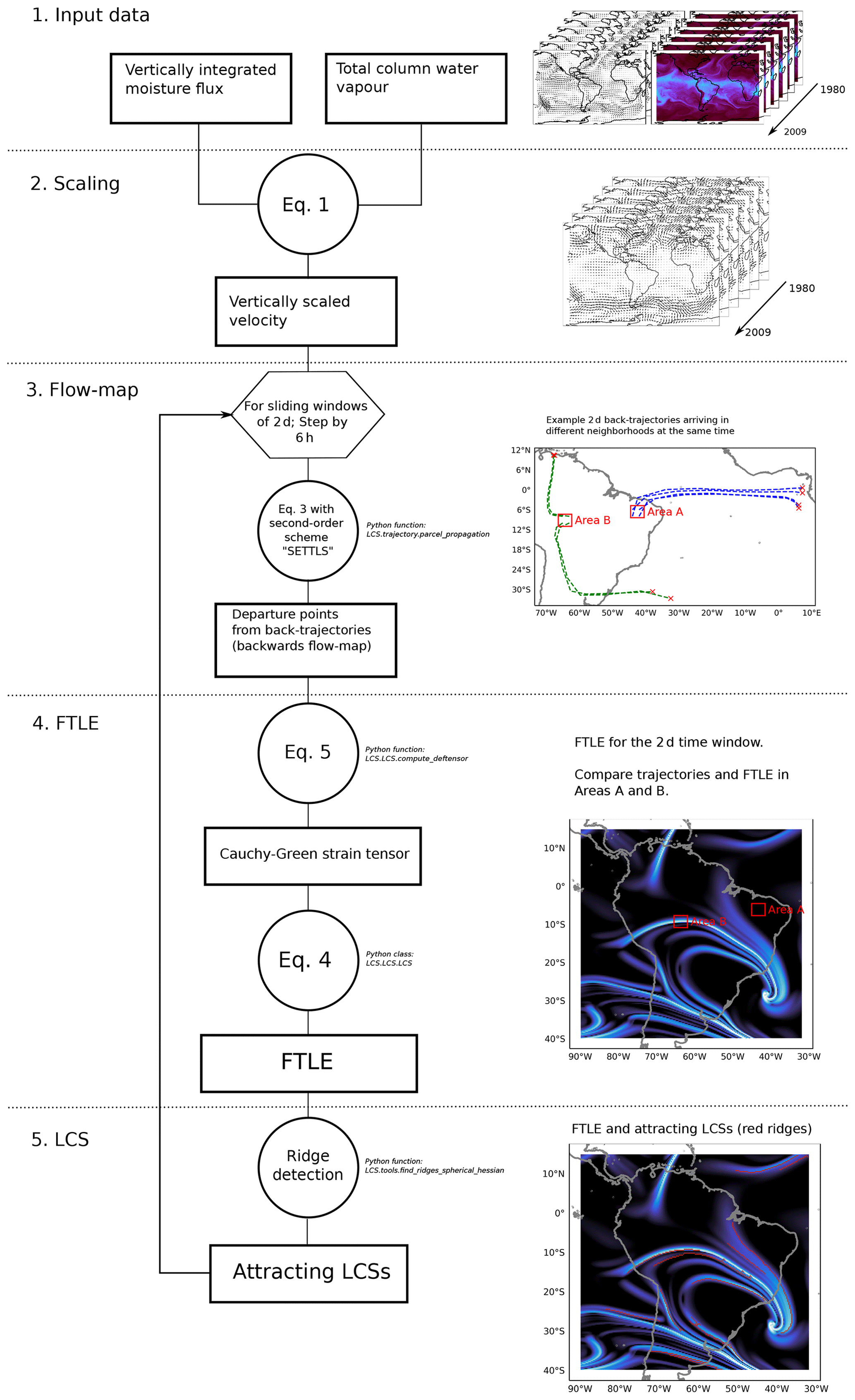
Figure 3 Schematic summary of the methodology employed to compute the FTLE and identify attracting LCSs. Corresponding Python classes and functions are referenced. See “Code and data availability” for repository link.

Table 1 Summary of the parameters employed to compute the FTLE and its ridges (LCSs).

4 Interpreting the FTLE scalar field and LCSs

An important distinction in this study is the one between the FTLE scalar field and the attracting LCSs represented by ridges in this field. The FTLE field at a given time depicts the state of mixing in a particular integration time interval. Relatively high FTLE in the backwards-in-time perspective reveals regions where mixing is stronger. In such regions, the departure distance among parcels back-advected from neighbouring arrival points is large. The FTLE represents this exponential folding rate along the principal axis of deformation. Regions where the FTLE is relatively low experience less mixing; i.e. arriving parcels departed from nearby locations. Ridges in this field correspond to the locally strongest attracting structures (i.e. attracting LCSs) associated with strong flow-map deformation. This relationship between trajectory deformation and the FTLE is exemplified in Fig. 3.

Figure 4a and b represent the zonal and meridional components of the 2 d backwards flow map on 24 January 2020 at 18:00 UTC. This event was classified by Brazilian meteorology agencies as a particularly strong SACZ associated with intense rainfall in southeast Brazil (CPTEC, 2020). The gradients of the departure positions represented in Fig. 4a and b are the components of the strain tensor C used to compute the FTLE scalar field in Fig. 4c. Filaments of high FTLE are immediately evident by visual inspection; ridges corresponding to attracting LCSs are highlighted in red.

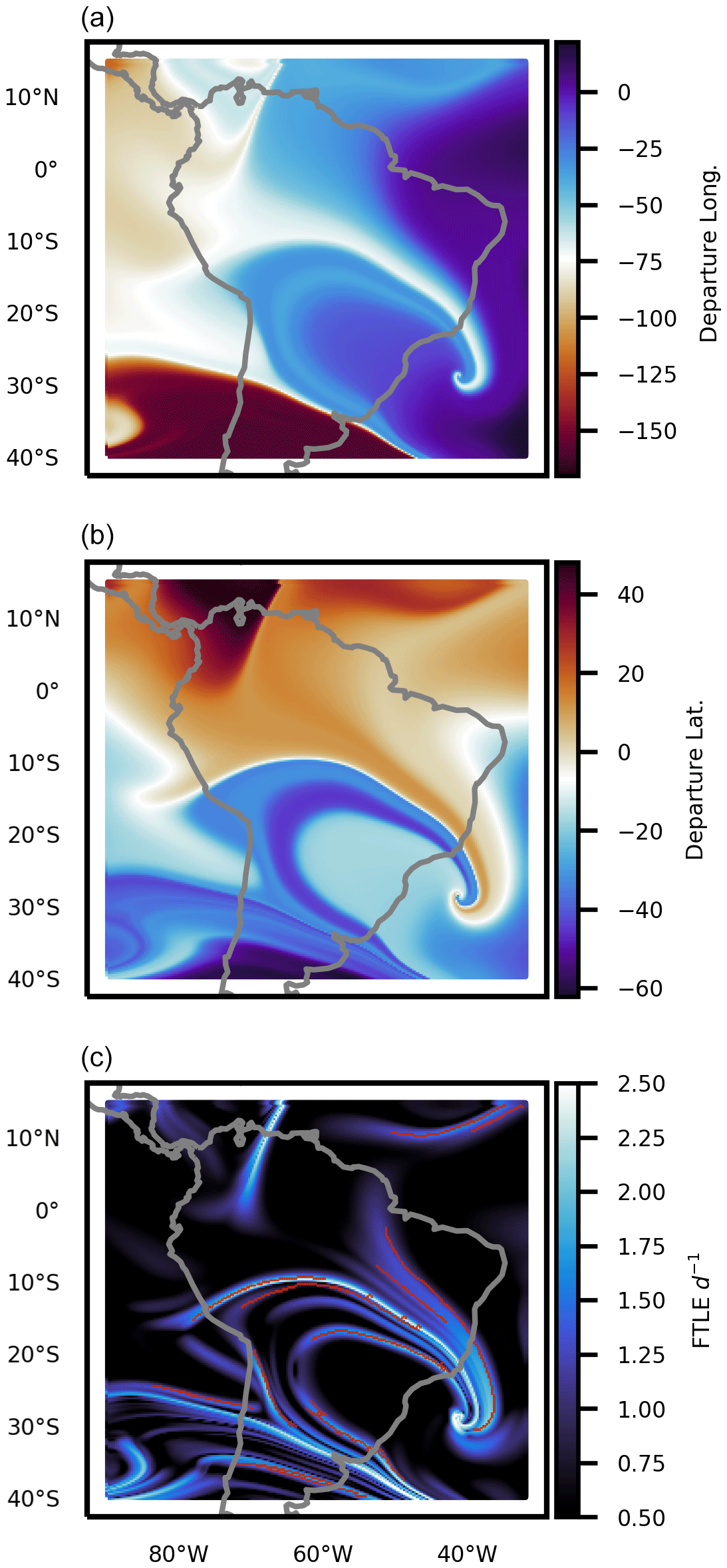
Figure 4 Example of the meridional (a) and zonal (b) components of the flow map, as well as the FTLE scalar field and convergence zones (c). Colours in panels (a) and (b) correspond to the departure longitudes and latitudes, respectively, of trajectories arriving on the ERA5 grid on 24 January 2020 at 18:00 UTC after advection by ${\mathit{V}}_{{\mathit{\rho }}_{\mathrm{v}}}$ for 2 d. Blue shades in panel (c) correspond to the 2 d FTLE (Eq. 4), and red lines correspond to height ridges, i.e. attracting LCSs. This day corresponds to the peak activity of an SACZ event.

The inspection of attracting LCSs and the flow-map components in Fig. 4 indicate that convergence zones represent interfaces of initially separated air masses. These interfaces can be visualised as sharp gradients of departure latitudes and longitudes. We highlight the sharp diagonal gradient in Fig. 4b across Brazil: parcels that originated in equatorial latitudes seem to face a transport barrier at about 10^∘ S; they are deflected east instead of proceeding to southern parts of the continent as they would in the climatological SAMS flow (Fig. 2). This suggests that such structures control the exchanges of moisture between the Amazon and southeastern/southern South America. In the next section we will examine this SACZ event in more detail and discuss how the LCSs relate with rainfall and moisture distribution.

5 LCSs, moisture and rainfall in a recent SACZ event

Attracting LCSs are structures that shape the evolution of passive tracers in time-dependent flows. Atmospheric moisture, however, is not a passive tracer, nor is it homogeneously distributed in the initial times of integration. Therefore, it is not guaranteed that flow entities such as attracting LCSs will shape moisture or rainfall in any meaningful way. In other words, the horizontal distribution of atmospheric moisture could be simply dominated by local sources and sinks. We know, however, from a climatological perspective that advection is important for the global hydrological cycle (Trenberth, 1999; Demory et al., 2014). In this section we explore the interplay of attracting LCSs, moisture and rainfall in a recent and significant SACZ event.

Figure 5 shows the evolution of attracting LCSs, total column water vapour, ${\mathit{V}}_{{\mathit{\rho }}_{\mathrm{v}}}$ and rainfall during an SACZ event in January 2020. In Fig. 5a, the SACZ is not yet formed and water vapour is roughly uniformly distributed around the continent. In the equatorial Atlantic, rainfall and moisture are closely aligned along an attracting LCS revealing the Atlantic ITCZ. In the South Atlantic (bottom-right corner of Fig. 5a), LCSs and rainfall appear near a cyclonic circulation. During the next day (Fig. 5b), an attracting LCS appears in western/central Brazil (label 1) as an interface along which northward flux from southern South America meets southward flux from the Amazon; they are both deflected east. This interface, identified by the LCS, appears to behave as a transport barrier to the climatological southward Amazonian moisture flux (Fig. 2) that supplies moisture to southern South America. In fact, this barrier (labels 1 to 5 in Fig. 5b–f) persists as total column water vapour remains low in southern South America.

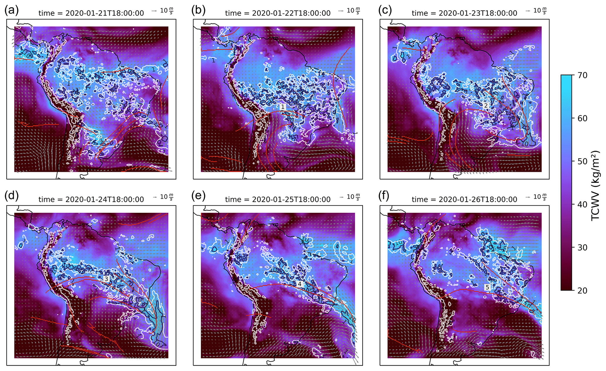
Figure 5 Rainfall (contours of 1, 5 and 10 mm h⁻¹), vectors of ${\mathit{V}}_{{\mathit{\rho }}_{\mathrm{v}}}$ and attracting LCSs (red lines) computed as ridges of the FTLE scalar field given by Eq. (4). Time labels are in UTC.

However, the LCSs in this case study are perhaps most evidently associated with the organisation of moisture and rainfall along a well-defined convergence zone. By definition, these LCSs are the locally strongest attracting structures; therefore, we expect that they are the cause of the well-organised rainfall bands in Fig. 5d–f. The initial situation of uniformly distributed moisture in Fig. 5a and scattered rainfall evolves into a situation where moisture and rainfall are narrowly distributed along attracting LCSs (Fig. 5d–f), forming a single diagonal band across the continent. The whole entity, which we may call the SACZ, stems from a favourable configuration of the large-scale mixing depicted by an ensemble of attracting LCSs. The attracting LCSs, in their turn, arise from large-scale stirring, caused by the motion of a cyclone.

Convergence features such as the SACZ are responsible for intraseasonal rainfall variability in South America and, in their turn, are subject to seasonal and interannual variations (Carvalho et al., 2004; Muza et al., 2009). In the following sections we provide a long-term analysis of the seasonal occurrence of LCSs in South America as well as their impact on intraseasonal rainfall and moisture flux variability.

6 Climatology and impact on rainfall and moisture

6.1 Frequency of occurrence

The annual and seasonal frequencies of occurrence of convergence zones defined as attracting LCS are shown in Fig. 6. Here the frequency of occurrence is computed as the number of LCS events in a grid box divided by the total number of time steps. A local maximum in the tropical Atlantic coincides with the climatological position of the ITCZ; its frequency increases in austral winter consistent with the increase in rainfall in the ITCZ (de Souza Custodio et al., 2017). Between 10 and 30^∘ S at 60^∘ W, there is a band of higher frequencies along the eastern side of the Andes in all seasons, coinciding with the SALLJ position (Montini et al., 2019). In austral summer, the frequency of convergence zones increases in southeast Brazil and the South Atlantic near the climatological SACZ position. The local frequency maximum in the South Atlantic (approx. 20^∘ S, 40^∘ W) is somewhat oriented along the coast. This could result from the interactions of the large-scale flow, sea breezes and coastal mountain ranges (Fig. 1), which contribute substantially to the wind and rainfall regimes in that region (Silva Dias et al., 1995; Perez and Silva Dias, 2017).

Figure 6 Annual (a) and seasonal (b) average frequency of occurrence of convergence zones defined as attracting LCSs between 1980 and 2009. Frequency of occurrence represents the number of LCS events in a grid box divided by the number of samples.

Given that LCSs frequent regions that coincide with the aforementioned rainfall mechanisms, we expect large-scale mixing to be playing a role in intensifying or generating these rainfall and moisture features such as the ITCZ or the SACZ. In the next section we quantify the local linear influence of mixing as measured by the FTLE on moisture and rainfall.

6.2 Correlation between the FTLE and rainfall

In this section we investigate how the FTLE correlates with rainfall and water vapour at grid-point scale during austral summer and winter. Since these are Eulerian quantities, a degree of care must be taken when interpreting these correlations. From the moisture budget, changes in the moisture content and rainfall are associated with moisture advection, mass convergence and evaporation in the immediate neighbourhood of the atmospheric column considered. The FTLE is a Lagrangian quantity representing the average deformation of arriving trajectories. It is only directly associated with Eulerian mass convergence in slowly varying or steady flows, where the Lagrangian strain can be approximated by the Eulerian strain (Ottino, 1989). Nevertheless, correlating the FTLE with rainfall and moisture is a simple way to quantify their dependence on mixing. Garaboa-Paz et al. (2017) have similarly correlated the FTLE with other atmospheric variables such as the Eady growth to identify the dependence of atmospheric rivers on the mixing variability.

Figure 7 shows the Pearson correlation coefficient between the FTLE, rainfall and total column water vapour at 2 d intervals in summer and winter. The 99 % confidence interval was calculated for the null hypothesis of zero correlation. Significant correlations are seen throughout most of the domain, indicating that the moisture content and rainfall in most regions are related, to some degree, to large-scale mixing. Two features of positive correlations are prominent in summer in Fig. 7a and b: a maximum in southeastern/central Brazil and a zonal band in equatorial northern/northeastern Brazil. Rainfall in these regions is directly influenced by the ITCZ and SACZ (Uvo et al., 1998; Ambrizzi and Ferraz, 2015). Negative correlations with total column water vapour in summer can be seen in the western Amazon (approx. 5^∘ S, 70^∘ W), indicating that the rainfall and moisture content rely on local sources or non-mixed (parallel trajectories) transport. In winter (Fig. 7c and d), the FTLE is positively correlated with rainfall in south Brazil; Paraguay and Uruguay are the most correlated with rainfall, while the storm track in the South Atlantic is where the positive correlation of FTLE with total column water vapour is highest.

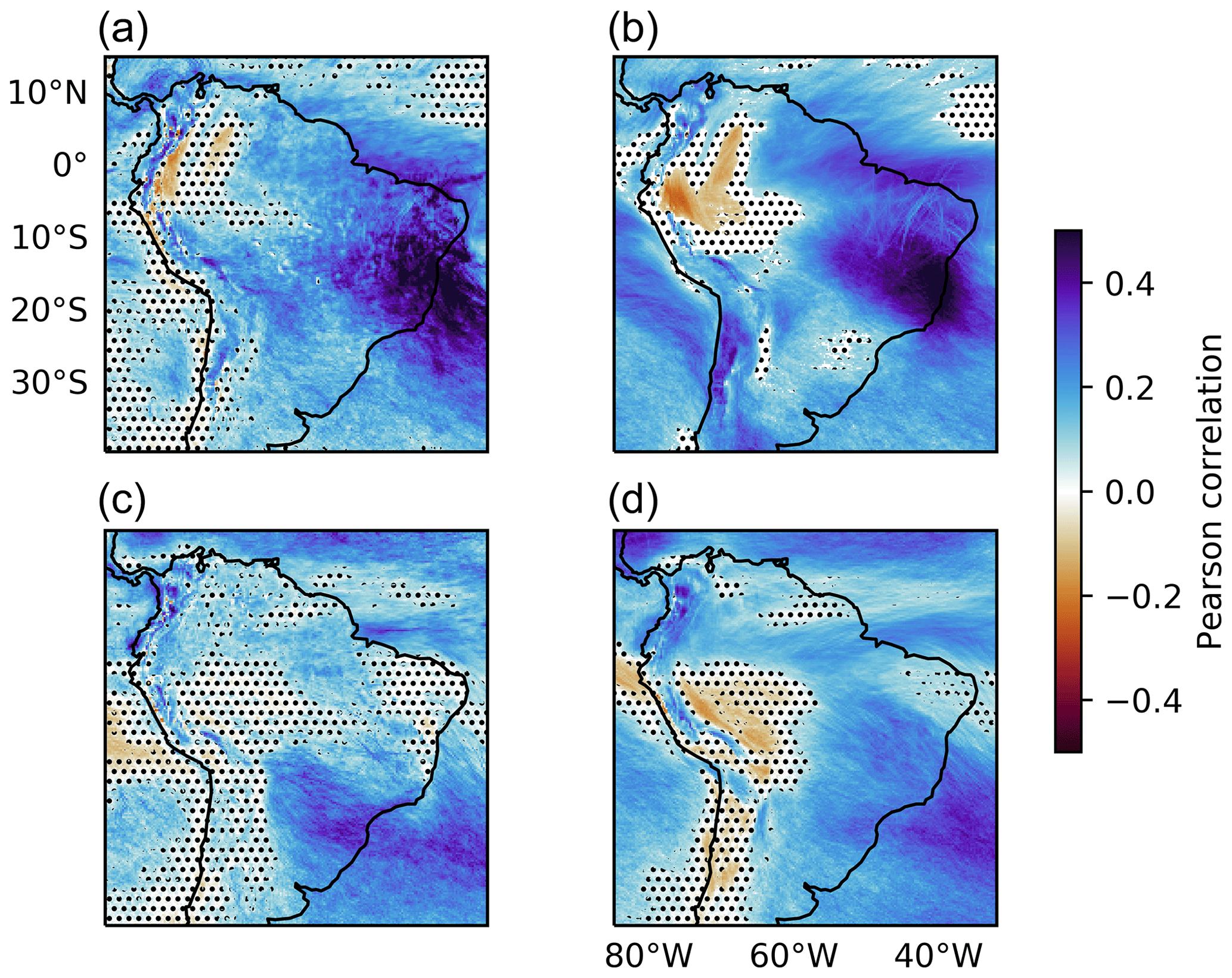
Figure 7 Pearson's correlation coefficient between the FTLE and rainfall (a, c) and total column water vapour (b, d) in DJF (a, b) and JJA (c, d). Correlations were computed in 6-hourly data. Stippled regions are inside the 99 % confidence interval for the null hypothesis of zero correlation.

While the FTLE scalar field presents significant grid-point correlations with rainfall and moisture, we expect that distinct features of large-scale mixing also influence these variables in the surroundings. For example, in the case study in Sect. 5 we have seen that LCSs intensified the moisture gradients and organised a continental-scale rainfall band. In the next section we investigate this regional impact of LCSs in intraseasonal variability by the composite analysis of LCS events on key regions in south and southeast Brazil.

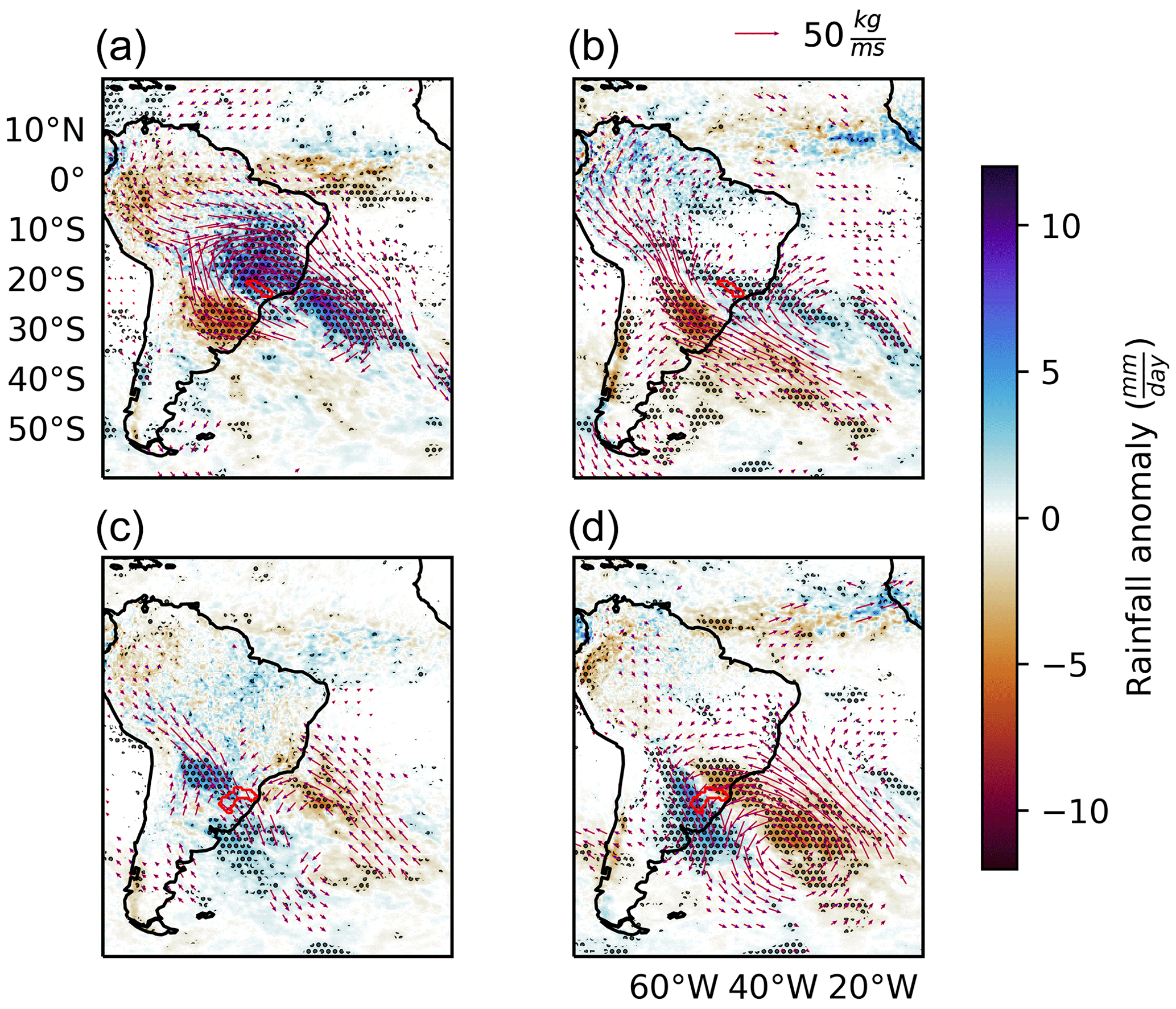
Figure 8 Anomalies of rainfall and vertically integrated moisture flux (vectors) during attracting LCS events in the Tietê (a, b) and Uruguay (c, d) basins in DJF (a, c) and JJA (b, d). Anomalies significant at the 99 % confidence level are stippled. The watershed boundaries are represented by red polygons.

6.3 Moisture flux and rainfall anomalies in the SACZ and the SALLJ regions

To investigate how the location of attracting LCSs influences rainfall and moisture transport variability, we focus on two watersheds that are tributaries of the La Plata River: Tietê and Uruguay. These basins were chosen because they are typically influenced by two of the mechanisms of interest: the SACZ in Tietê and the SALLJ in Uruguay. Economic activity in both watersheds depends on rainfall particularly due to hydroelectric power generation and agriculture. Moreover, a number of densely populated cities, including São Paulo, are located in the Tietê catchment area.

Figure 8 shows the anomalies of rainfall and vertically integrated moisture flux in summer and winter during events of attracting LCSs over the Tietê and Uruguay watersheds. The events were selected when LCSs intersected the watershed areas. In summer in the Tietê basin (Fig. 8a), attracting LCS events are associated with a significant anomalous rainfall dipole and cyclonic moisture flux. North of the basin, positive rainfall anomalies form a diagonal band extending from central Brazil to the South Atlantic; to the south, there is a negative rainfall anomaly. Similar anomalies were associated with the SACZ by Muza et al. (2009). A northward anomalous flux along the Andes indicates a weaker SALLJ during attracting LCS events in Tietê. This is also noticed in winter (Fig. 8b), although the positive rainfall anomalies are weaker and the cyclonic anomaly is centred in the South Atlantic. The SALLJ weakening could produce the significant negative rainfall anomalies near south Brazil and Paraguay. This interplay between the SACZ and SALLJ is a documented feature of the South American climate (Boers et al., 2014).

During LCS events in the Uruguay basin (Fig. 8c and d), there is an anti-cyclonic moisture flux anomaly in the South Atlantic associated with a southward flux along the Andes, indicating stronger SALLJ. The rainfall anomalies are positive near south Brazil, Uruguay and Paraguay. Liebmann et al. (2004) found similar rainfall anomalies of about 4 mm d⁻¹ in the vicinity of the Uruguay basin during strong SALLJ events.

The consistency of the anomalies in Fig. 8 with previous studies about the SACZ and SALLJ highlights the potential of the methodology to identify important mechanisms of moisture transport. Moreover, it indicates that the SACZ and the SALLJ, from a kinematical point of view, are similar coherent structures stemming from large-scale mixing. This raises a question about the dynamical mechanisms that create these kinematical features. Both the SACZ and the SALLJ have been associated with teleconnection patterns across the Pacific; thus, in the next section we verify if LCS events in the Tietê and Uruguay basins are associated with similar dynamical settings.

6.4 Dynamical mechanisms of LCS in the SACZ and the SALLJ regions

Figure 9 shows the geopotential anomalies at 250 hPa in summer and winter during LCS events in the Tietê and Uruguay basins. During events in Tietê in summer (Fig. 9a and c), an anomalous trough is positioned south of the watershed roughly aligned with the cyclonic circulation in Fig. 8a. This trough is connected with a wave pattern that appears to propagate from the South Pacific (Fig. 9c). This observation is consistent with the mechanism of SACZ formation proposed by Van Der Wiel et al. (2015) based on ray-tracing diagnostics of Rossby waves initiated by a heat source in the same location. Anomalous convective activity in the western Pacific and a pulse of the Madden–Julian Oscillation have also been reported to create similar wave-train patterns (Cunningham et al., 2006; Grimm, 2019).

Figure 9 Geopotential height anomalies at 250 hPa during attracting LCS events in the Tietê (a–d) and Uruguay (e–h) basins during the austral summer (DJF) and winter (JJA) for lags 0 and −3 d. Anomalies significant at the 99 % confidence interval are stippled. Red polygons represent the watershed boundaries.

In winter in Tietê (Fig. 9b and d), a wave pattern arises similar to the Pacific–South Atlantic teleconnection (Ambrizzi et al., 1995), positioning a trough south of the Tietê watershed. This trough is slightly to the east (downstream) of the anomalous low-level circulation in Fig. 8b, indicating baroclinicity. This type of configuration has been noted as a cyclogenesis mechanism in southeast and south Brazil (Crespo et al., 2020). During LCS events in the Uruguay basin in both seasons (Fig. 9e and f), an anomalous 250 hPa ridge is positioned in the South Atlantic, aligned with the anti-cyclonic circulation in Fig. 8c and d. The lagged anomalies (Fig. 8g and h) indicate that this ridge originates from a perturbation in higher latitudes.

These geopotential anomalies associated with LCS events indicate that large-scale dynamical mechanisms are providing a favourable kinematical configuration for the development of LCSs and the further organisation of moisture and rainfall in bands. This is consistent with the discussion in Shepherd et al. (2000) that increased Rossby wave activity changes the kinetic energy spectrum such that coherent structures of tracer accumulation are more likely to appear.

7 Summary and conclusions

This is the first study to investigate the role of Lagrangian coherent structures (LCSs) in tropical and subtropical rainfall. We defined skeletons of atmospheric convergence zones as attracting LCSs given by ridges of the finite-time Lyapunov exponent (FTLE). The FTLE is a measure of deformation among neighbouring trajectories that synthesises the state of mixing in fixed time intervals and allows the visualisation of transport barriers. Defining convergence zones as attracting LCSs is consistent with a Lagrangian understanding of convergence zones as regions where remotely sourced air masses interact (Simpson, 1947). This definition also implies that convergence zone skeletons are associated with tracer accumulation, potentially explaining the organisation of cloud and rainfall bands.

Attracting LCSs frequent tropical and subtropical South America, with climatologies consistent with previous studies of large-scale phenomena such as the Intertropical Convergence Zone, the South Atlantic Convergence Zone (SACZ) and the South American Low-Level Jet (SALLJ). Point-by-point correlations showed that, in the typical areas of action of these mechanisms, moisture and rainfall depend to some extent on the large-scale mixing represented by the FTLE scalar field.

Fixing locations of interest in watersheds in south and southeast Brazil, we showed that significant rainfall and moisture flux anomalies are associated with attracting LCS events. These anomalies are consistent with previous climatologies (e.g. Boers et al., 2014) of the SACZ and the SALLJ. We also analysed geopotential anomalies at 250 hPa during LCS events in these two basins. The geopotential composites suggest that remotely sourced perturbations are stirring the low-level synoptic-scale flow such that attracting LCSs arise and organise the moisture transport and rainfall in fine bands. This behaviour resembles the spectrally non-local regime in the stratosphere, where the evolution of tracer features is set by low wavenumber perturbations (Shepherd et al., 2000).

In the case of the SACZ, our approach differs substantially from existing classifications that equate the SACZ to patterns associated with convective or rainfall variability (Carvalho et al., 2004; Ambrizzi and Ferraz, 2015). Our approach first asserts the existence of coherent flow features organising atmospheric moisture. Only then do we associate them with rainfall variability. Because of that, the approach is general and may be applied in other locations to identify similar structures. Nonetheless, our results are consistent with the current understanding of the main features of the SAMS (Marengo et al., 2012), supporting that the methodology can be employed as a detection criterion for these features, particularly the SACZ. Such objective classification of convergence zone skeletons could assist operational weather forecasters in identifying these weather systems. By considering the mean FTLE along an LCS, the forecaster could estimate their potential to intensify moisture gradients, thus anticipating the development of rain bands or moisture channels.

For future developments, we suggest refining the classification by allowing different types of convergence zones. This could be done by analysing physical quantities across and along the attracting LCSs. For example, if the temperature gradient is strong perpendicular to the FTLE ridge, such convergence zone could be associated with a frontal system. Similarly, a convergence zone could be associated with orography if the LCS is parallel to elevation features. Alternatively, convergence zones could be filtered by properties of the arriving parcels, such as temperature and water vapour concentration, likewise the trajectory filtering available in LAGRANTO (Sprenger and Wernli, 2015). This refined classification would help understand the mechanisms that generate the LCSs and, ultimately, organised rainfall bands. As a final goal, the proposed framework could serve as basis for a global criterion for convergence zones, replacing or being combined with region-specific classification methods.