the Creative Commons Attribution 4.0 License.
the Creative Commons Attribution 4.0 License.
 | 02 Dec 2022
Reanalysis representation of low-level winds in the Antarctic near-coastal region
Stavroula Biri
Thomas J. Bracegirdle
John C. King
Elizabeth C. Kent
Étienne Vignon
John Turner
Low-level easterly winds encircling Antarctica help drive coastal currents which modify transport of circumpolar deep water to ice shelves, and the formation and distribution of sea ice. Reanalysis datasets are especially important at high southern latitudes where observations are few. Here, we investigate the representation of the mean state and short-term variability of coastal easterlies in three recent reanalyses, ERA5, MERRA-2 and JRA-55. Reanalysed winds are compared with summertime marine near-surface wind observations from the Advanced Scatterometer (ASCAT) and surface and upper air measurements from coastal stations. Reanalysis coastal easterlies correlate highly with ASCAT (r= 0.91, 0.89 and 0.85 for ERA5, MERRA-2 and JRA-55, respectively) but notable wind speed biases are found close to the coastal margins, especially near complex orography and at high wind speeds. To characterise short-term variability, 12-hourly reanalysis and coastal station winds are composited using self-organising maps (SOMs), which cluster timesteps under similar synoptic and mesoscale influences. Reanalysis performance is sensitive to the flow configuration at stations near steep coastal slopes, where they fail to capture the magnitude of near-surface wind speed variability when synoptic forcing is weak and conditions favour katabatic forcing. ERA5 exhibits the best overall performance, has more realistic orography, and a more realistic jet structure and temperature profile. These results demonstrate the regime behaviour of Antarctica's coastal winds and indicate important features of the coastal winds which are not well characterised by reanalysis datasets.
- Article
(16095 KB) - Full-text XML
-
Supplement
(11108 KB) - BibTeX
- EndNote


Easterly winds prevail over most of coastal Antarctica and extend up to about 2 km above surface level. Easterly wind stress is in turn an important driver of the westward Antarctic Coastal Current, a circulation coupled in many regions to the Antarctic Slope Front (ASF) between shelf waters and warmer circumpolar deep water (Thompson et al., 2018). The Southern Ocean meridional overturning circulation may respond more to changes in Antarctic coastal winds (or “polar easterlies”) than to the westerlies further north (Stewart and Thompson, 2012). It has been shown that modifications to easterly wind stress and Ekman pumping near the coast could enhance subsurface advective heat fluxes across the ASF, contributing to ice shelf basal melt (Spence et al., 2014; Goddard et al., 2017; Stewart et al., 2019). Antarctic coastal winds also have a large non-easterly component, especially on short timescales. Meridional winds could act as a control on ice shelf stability in some regions (Hazel and Stewart, 2020) and have a major impact on sea ice concentrations, for example off the Ross Ice Shelf (Kurtz and Bromwich, 1985; Petrelli et al., 2008; Mathiot et al., 2012; Silvano et al., 2020), and in other prominent regions of sea ice production (Wang et al., 2021). Given the sparsity of nearby observations, reanalysis datasets are critical for characterising Antarctic coastal winds, and often provide boundary conditions for atmospheric and ocean models. As an observational benchmark they are also important for evaluation of coupled models used for future projections.
In part due to the paucity of assimilated observations, historical trends of coastal winds from reanalysis are uncertain and differ among datasets, though all indicate an increase in the seasonality of the easterlies over the last few decades (Hazel and Stewart, 2019). Over Antarctica itself, the magnitude of the late 20th century trend in near-surface winds differs considerably in its pattern and magnitude between reanalyses, especially in the coastal region (Dong et al., 2020). On average, reanalyses exhibit higher wind speed correlation coefficients with surface station measurements in summer compared to winter and over inland regions compared to the coast (Tetzner et al., 2019; Dong et al., 2020). The realism of tropospheric wind profiles is improved in the more recent ERA5 reanalysis with respect to the earlier ERA-Interim at coastal stations, but large deficiencies remain (Vignon et al., 2019). Reanalysis evaluations have tended to focus on the onshore coastal region, in part due to the limited availability of satellite observations near the coast (Bourassa et al., 2019), but since offshore winds play a key role in interactions between the atmosphere, ocean and cryosphere, an evaluation of performance against observations from the marine coastal sector is needed.
Alongside the lack of evaluation offshore, relatively little attention has been given to reanalysis representation of wind variability and extremes. Jones et al. (2016) show how considerable underestimation of low-level wind speeds occurs in the Amundsen Sea Embayment when a “low-level jet” is present, reminiscent of underestimated elevated wind speeds in regions of complex orography in the Arctic (e.g. Moore et al., 2016). Extreme coastal winds are important for rapid sea ice loss (Jena et al., 2022) and calving events (Francis et al., 2021), so a characterisation of reanalysis performance during high-wind states is needed. However, Antarctic coastal winds are influenced by a range of drivers, each of which presents a different set of challenges for reanalysis representation. Although mean coastal wind speeds peak onshore, the variability on 12-hourly timescales is highest just offshore where the interaction between directionally-constant continental winds and highly variable synoptic flows becomes important (Fig. 1). One important driver is katabatic forcing, which sustains shallow terrain-following drainage flow towards the coast (Ball, 1960; Parish and Bromwich, 1987) but its flow often stops abruptly at the coastal margin (e.g. Yu and Cai, 2006; Tomikawa et al., 2015; Vignon et al., 2020) and its behaviour in models is sensitive to the representation of the atmospheric boundary layer (King et al., 2001; Parish and Cassano, 2003; Orr et al., 2014). As a result, the indirect effect of katabatic forcing on offshore flow, for example due to momentum advection, is uncertain. Representation of orography is important as long-wave cooling over the steep coastal slopes sets up both katabatic flows near the surface and a deeper layer of terrain-following isentropes above it which explains the easterly “low-level jet” structure (Fulton et al., 2017). Orography is also critical for blocking and barrier winds induced by steep Antarctic coastal slopes (Parish and Cassano, 2001, 2003; Orr et al., 2014; Weber et al., 2016; Yamada and Hirasawa, 2018). Other drivers include the large-scale pressure gradient force (van den Broeke and van Lipzig, 2003) and, on shorter timescales, synoptic storms.
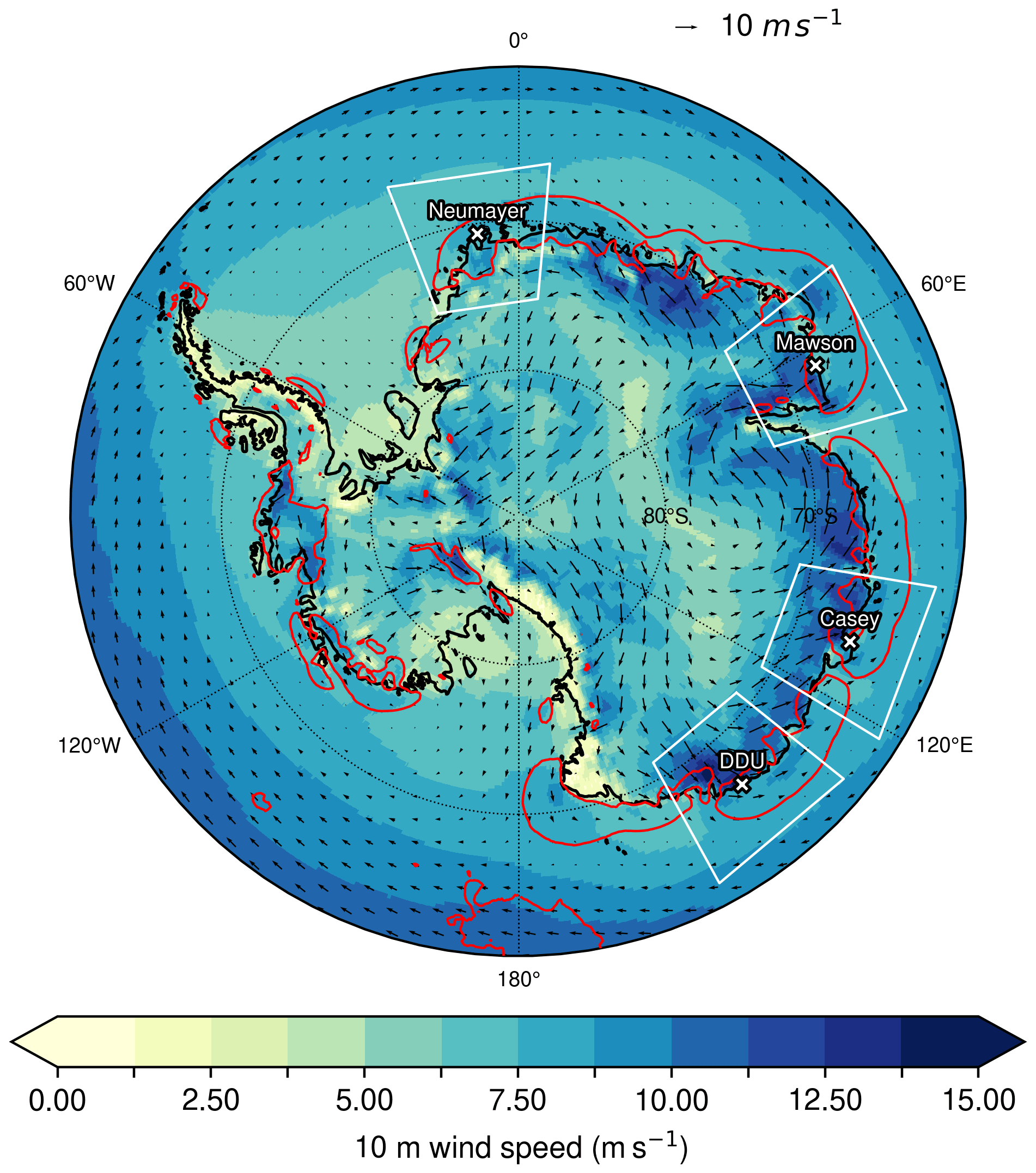
Figure 1Mean ERA5 10 m wind speed for the period January 2010 to December 2017 (shaded). The 4 m s−1 contour of the standard deviation of 12-hourly 10 m wind speed for the same period is overlain in red. White boxes indicate the regions selected for the SOM analysis, with labelled station locations. The arrows represent vector average wind speed, and thus go to zero length in regions with zero directional constancy.
In this paper, we aim to provide both a representative overview of reanalysis performance in the coastal easterly sector but also to test whether that performance is sensitive to short-term variations in the large-scale pressure conditions driving the coastal winds. By comparing reanalysis performance across driving states and geographic locations, we aim to shed light on possible sources of error and offer a process-oriented perspective to help select the most appropriate reanalysis to use when characterising the Antarctic coastal easterlies. Throughout this paper, we refer to “synoptic” and “katabatic” forcing to characterise short-term variability. By “synoptic” we are referring to variations in flow linked to large-scale pressure gradients (order of 1000 km) set up over a timescale of days, for example due to the passage of low pressure systems. “Katabatic” forcing is instead associated with near-surface thermodynamic processes driving downslope flow, with uncertain variability through time.
The research in this paper is guided by three questions:
-
How well do reanalyses represent the spatial patterns and short-term variability of near-surface winds within the Antarctic coastal easterly sector?
-
To what extent is reanalysis representation of Antarctic coastal winds sensitive to variations in the driving flow regime?
-
Which reanalysis most accurately represents Antarctic coastal winds?
Our analysis has two components; firstly, to quantify reanalysis performance across the entire coastal region we compare with observations from the EUMETSAT MetOP-ASCAT sensor, which has near-coastal data available during austral summer. Next, to evaluate reanalysis representation of variability on short timescales, a self-organising map (SOM) methodology is used to composite surface and upper air wind data available from four coastal surface stations which have high-resolution radiosonde data compiled by Vignon et al. (2019).
Section 2 details the datasets used as well as the collocation and SOM approach. Results are presented in Sect. 3, including an evaluation against ASCAT (Sect. 3.1) and a SOM-based evaluation against station measurements (Sect. 3.2). Results are discussed and an overall assessment of reanalysis reliability is given in Sect. 4 with conclusions in Sect. 5.
2.1 Reanalysis datasets
For this analysis, we evaluate ERA5, MERRA-2 and JRA-55, which belong to the latest generation of reanalyses which have been widely adopted for studies of the Antarctic circulation and for quantifying historical trends and evaluating climate models. Near-surface winds are evaluated against in situ and scatterometer-derived winds for the period January 2010 to December 2017. For the comparison with scatterometer winds, the reanalysis neutral 10 m winds are used. This is because the same assumption of a neutral profile is made when deriving ASCAT 10 m winds from surface stress (the feature directly observed by scatterometers) so, as in the ECMWF assimilation scheme Hersbach (2010), we consider them to be more comparable.
2.1.1 ERA5
ERA5 is the fifth generation in the European Centre for Medium-range Weather Forecasts (ECMWF) series of reanalyses. A full technical description of the setup is given by Hersbach et al. (2020). The dataset is derived using a 2016 version of the operational ECMWF Integrated Forecasting System (IFS) model (cycle 41r2) and a hybrid incremental 4D-Var data assimilation methodology. ERA5 is available on a regular 0.25∘ grid at 31 km horizontal grid spacing and on 137 vertical levels. Both surface-level diagnostics and data on pressure levels are available hourly. A final release of ERA5 is publicly available for 1959 onwards. ERA5 near-surface winds are a diagnostic derived in IFS output by scaling the winds at the 40 m height level to 10 m assuming a roughness length for short grass (0.03 m) when the surface roughness is less than or equal to 0.03 m and otherwise using the tile roughness length. For our comparison with ASCAT ocean winds, the ERA5 10 m neutral wind product is used instead, which is derived from surface stress using the tile roughness length and assuming neutral stability.
2.1.2 MERRA-2
The Modern-Era Retrospective Analysis for Research and Applications, version 2 (MERRA-2) has been developed by NASA's Global Modeling and Assimilation Office (GMAO) as an intermediate reanalysis intended to incorporate updates to GMAO modelling and data assimilation into the MERRA framework (Gelaro et al., 2017). MERRA-2 is based on the Goddard Earth Observing System-5 (GEOS-5) forecast model and is available from 1979 on an approximately grid (50 km grid spacing) with 72 vertical levels. Surface fields (including 10 m wind speed) are available hourly, with 3-hourly vertical fields on pressure levels. Wind speeds at 10 m are derived in MERRA-2 by interpolating from the lowest model level using Monin–Obukhov similarity theory, thereby accounting for the effects of varying near-surface atmospheric stability (Torralba et al., 2017). These stability-dependent winds are compared with station measurements. For comparison with ASCAT, we calculated 10 m neutral wind speeds using the hourly output of friction velocity (u∗) and roughness length (z0 m) from the MERRA2 flux diagnostics (GMAO, 2015c) following
where k=0.4 is the von Kármán constant.
2.1.3 JRA-55
The Japanese 55-year Reanalysis (JRA-55) developed by the Japan Meteorological Agency (JMA) covers a period from 1958 onwards and is an update to JRA-25, incorporating novel observations and a 4D-Var data assimilation system (Kobayashi et al., 2015). The JMA global spectral model (GSM) is used as the underlying forecast model. The JRA-55 grid corresponds to approximately 55 km horizontal grid spacing, with 60 vertical levels. Surface fields are available on 6-hourly timesteps, so compared to ERA5 and MERRA-2, the comparison with relatively infrequent scatterometer observations is more limited (Sect. 2.2.1). JRA-55 10 m winds are interpolated from the lowest model level as in MERRA-2, but unlike the stability-dependent ERA5 and MERRA-2, near-surface winds are calculated assuming neutral stability in the surface layer (Torralba et al., 2017).
2.2 ASCAT
Remote Sensing Systems (RSS, http://www.remss.com, last access: 11 August 2021) use radar backscatter data from the EUMETSAT MetOP-ASCAT sensor to derive near-surface wind vectors at 10 m height above sea surface over ice-free open water surfaces from 1 March 2007 onwards on a Cartesian grid (Ricciardulli and Wentz, 2016) with good coverage of polar latitudes. The open-ocean backscatter data are converted into winds using a geophysical model function (GMF). Advanced Scatterometer (ASCAT, version 2.1) is a C-band scatterometer used to measure surface radar backscatter along two swaths each ∼500 km wide separated by a 360 km gap processed to provide wind vectors for a grid spacing of about 25 km. The data contain a rain flag, since rain can produce a positive bias at low wind speeds due to backscatter from rain drops and negative bias at high wind speeds due to atmospheric attenuation of the signal. Undetected sea ice can limit the quality of scatterometer data and wind speeds higher than 35 m s−1 (Ricciardulli and Wentz, 2016). Belmonte Rivas and Stoffelen (2019) report that the magnitude of ASCAT wind component errors on the scatterometer measurement globally is ∼0.7 m s−1 with negligible bias. We use ASCAT to evaluate reanalysis near-surface winds offshore, but it is important to note that ASCAT wind observations are assimilated into all three reanalyses used in this paper from 2008. A close correspondence between ASCAT and the reanalyses is expected therefore. Remaining differences could be due to large biases in the first guess model, inadequacies in the assimilation system, scale mismatches and inclusion of observations in our results which were not assimilated by the respective reanalyses. We do not intend to provide an independent evaluation of skill using ASCAT, but instead to compare between reanalyses, and to highlight aspects of the observed wind field and variability which are not captured by the reanalyses in spite of the observational constraints applied.
Collocation of reanalyses and ASCAT
For comparison, the reanalysis winds were mapped to the ASCAT grid by selecting the nearest neighbour in space and time and requiring a time match within an hour. To collocate spatially, we remap the reanalysis data onto the ASCAT grid using a nearest neighbour interpolation scheme. Every ASCAT swath pair has a different overpass time with the observation times of ascending and descending pass segments being interleaved throughout the day. For the collocation in time, we first round the time of each ASCAT observation to the nearest full hour and store these values as an array. Then for each grid point we collocate the rounded timestep in the array with the timestep in the reanalysis for the same point. The time resolution for JRA-55 is coarser (6 hourly), thus the rounded ASCAT timestep can only be “matched” on four timesteps (i.e. 00:00, 06:00, 12:00, 18:00), and as a result certain overpasses cannot be collocated following our time-collocation methodology. The points that cannot be collocated are left missing.
Analysis is primarily constrained to austral summer due to the seasonal expansion of sea ice which prevents wind speed observations near the coast. A breakdown of the results by season is given in Sect. S2 (Supplement).
2.3 In situ wind observations
Surface (10 m) and upper air (radiosonde) wind observations from four representative permanent East Antarctic sites are used. These include Neumayer on the Ekström Ice Shelf and three stations at the foot of steep coastal slopes, Mawson, Casey and Dumont d'Urville (DDU) (Fig. 1). 10 m wind speed measurements from surface stations are withheld from assimilation into JRA-55, MERRA-2 and ERA5 (Kobayashi et al., 2015; Gelaro et al., 2017; Hersbach et al., 2020), but the local wind field is not entirely independent from observations due to the assimilation of upper air wind, pressure and temperature profiles. Surface meteorological observations were obtained via the SCAR READER database (Turner et al., 2004). Neumayer, Mawson and DDU were selected for this analysis to evenly sample the East Antarctic coastline and due to their high representativeness of the coastal lower troposphere (see Vignon et al., 2019, Fig. 11). Casey, on the other hand, is less representative but is situated near complex orography which is represented differently in the three reanalyses (see Sect. 2.3.1). Long-term vertical profile data from West Antarctica are currently lacking but would be highly valuable for an evaluation of reanalysis performance of this kind, for example under various configurations of the Amundsen Sea Low.
High-resolution vertical wind profiles measured with Vaisala RS-92 radiosondes (Modem M2K2-DC at DDU) from the dataset collated by Vignon et al. (2019) are used, with technical details described in Sect. 2.1 therein. Important post-processing steps include calculation of measurement heights using a standard hydrostatic approximation based on temperature, humidity and pressure readings (König-Langlo et al., 1998), followed by linear interpolation to 10 m resolution from data available at 1 s intervals at Mawson, DDU and Casey, and 5 s intervals at Neumayer. Following Vignon et al. (2019), the lowest 100 m of data are not used due to possible thermal lag error (e.g. the radiosonde not equilibrating with outdoor temperatures prior to launch) and to allow the balloon to reach ambient flow velocity.
Collocation of reanalyses and station measurements
Comparison of gridded datasets with point observations is not straightforward, especially in regions of complex orography or where steep slopes generate an offset between the actual station elevation and that at the station location in the model (Dong et al., 2020). In this evaluation we compare station observations with the nearest reanalysis grid point for both the surface and upper air data as in a number of previous analyses (Jones et al., 2016; Gossart et al., 2019; Tetzner et al., 2019; Vignon et al., 2019). Within the lowest 3000 m, sondes do not generally drift more than a few kilometres horizontally (Vignon et al., 2019, Appendix C) so we do not account for sonde drift in this analysis. We recognise that the chosen grid point may not be fully representative of the local conditions at the station however. To explore this further, we map the correlation between measured 10 m near-surface winds and all nearby grid points (Fig. 2).
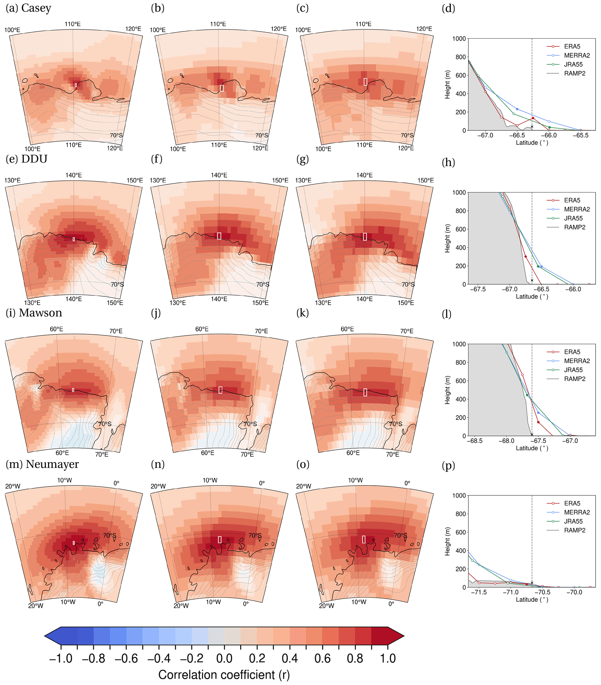
Figure 2Three left columns (ERA5 leftmost, MERRA-2 in the centre and JRA-55 the rightmost) show correlations between 10 m wind speed measured at surface stations with the local 10 m reanalysis wind field, with the selected nearest neighbour reanalysis grid point outlined in white. Rightmost column shows south–north cross sections through the location of the station, with orography from the RAMP2 dataset shaded in grey, and reanalysis orography from ERA5 (red), MERRA-2 (blue) and JRA-55 (green) indicated as a line. Filled markers on the lines mark the respective nearest neighbour reanalysis grid point. Shown are Casey (a–d), DDU (e–h), Mawson (i–l) and Neumayer (m–p).
Correlations between reanalysis and station 10 m wind speeds (Fig. 2, three left columns) are high over a large region surrounding most stations, suggesting local factors do not dominate the observed winds so a comparison with coarser gridded data is meaningful. A possible exception to this is Casey (Fig. 2a–c), where although correlations close to the station are high, shifting the selected reanalysis grid point slightly could have a large impact upon results. This is likely due to the Law Dome east of Casey (66∘ S, 112∘ E) which, at a peak altitude of 1395 m, is both a barrier to the large-scale flow and a likely source of topographically induced gravity waves with highly localised effects (Murphy and Simmonds, 1993; Turner et al., 2001; Adams, 2004). All reanalyses include some representation of the Law Dome but in ERA5 the peak rises to 1259 m compared to 964 m in MERRA-2 and 952 m in JRA-55.
Orographic slopes from the plateau to the coast differ considerably between reanalyses (Fig. 2, rightmost column). All three datasets have orography that is noticeably smoothed compared to the 1 km Radarsat Antarctic Mapping Project digital elevation model (DEM) version 2 (RAMP2) (Liu et al., 2015). ERA5 orography is derived from RAMP2 south of 60∘ S and so is closest to this benchmark, but in general the slope gradient is not as steep meaning the altitude of the matched grid point is greater than the station altitude along the coastal slopes and approximately equal (within 60 m) at Neumayer on the flat Ekström Ice Shelf.
To test the sensitivity of the results to grid point collocation, the analysis was repeated with station wind data matched to each of the two grid points immediately north and south of the nearest neighbour (i.e. the grid box outlined in white in the three left columns of Fig. 2), with results described in Appendix A. In brief, the value of the bias for states with a primarily katabatic influence is very sensitive to this collocation test due to the sharp cutoff which occurs at the coast, but other performance characteristics and the differences between stations are robust.
2.4 Self-organising maps
Wind field variability local to observing stations is characterised in this study using self-organising maps (SOMs). The goal is to group periods with similar local pressure conditions, including the magnitude, gradient and orientation, without needing to create a priori metrics to distinguish them. SOMs are a data-driven approach used to cluster multidimensional data into similar groups arranged in a 2D grid with a user-specified number of “nodes”. A summary of the unsupervised learning algorithm applied in a climate context is given by Skific and Francis (2012). The iterative SOM approach allows non-linearities in the data distribution to be accounted for, compared for instance to a principal component analysis which produces linear combinations of features in the data space (when the important underlying patterns may not in fact vary linearly). The main advantage of SOMs over other similar techniques is that nearby nodes are updated during training such that in the final set of nodes similar patterns or states are grouped together. Examples of use in an Antarctic context include the study of patterns and drivers of the Ross Ice Shelf Airstream (Nigro and Cassano, 2014b, a) and evaluation of the Antarctic Mesoscale Prediction System (AMPS) against station data (Jolly et al., 2016), with similar clustering techniques used to classify synoptic states associated with Antarctic surface melt episodes (Scott et al., 2019).
SOMs in our analysis are driven using the 12-hourly ERA5 mean sea level pressure (MSLP) field over a 200×200 km grid centred upon the location of each station for 2010–2017. Each 12-hourly MSLP field in ERA5 is then matched to the closest SOM node (lowest squared difference) to determine a set of dates for each SOM. Observations and reanalysis winds are then composited by these dates. 12-hourly data are used to match the approximate frequency of sonde launches at coastal stations. SOMs are calculated using the Somoclu library for Python: https://somoclu.readthedocs.io/en/stable/download.html (last access: 15 November 2022; Wittek et al., 2017).
Several metrics are used to determine the appropriate number of SOM nodes. With fewer nodes, the SOM representation of synoptic states may be too generalised. Conversely, with a larger array, duplicates are introduced (Cassano et al., 2015; Gibson et al., 2017) though how undesirable this is depends on the application (Hewitson and Crane, 2002). The similarity among SOM nodes, similarity of the composited wind fields, and correlations between data points (in this case 12-hourly MSLP fields) and their respective SOMs are quantified for various configurations in Fig. B1. Appendix B also provides further details on the selection of SOM configuration. Here, we use six SOM nodes (organised onto a 2×3 grid) which represents approximately four states with relatively strong synoptic forcing, and two with weaker forcing and conditions favouring katabatic low-level winds of continental origin.
The period 2010–2017 is used in this analysis for several reasons. Firstly, Neumayer station is in a fixed position on the ice shelf throughout this period (Neumayer Station III data available since February 2009). Secondly, surface anemometer instrumental models are mostly consistent through this period (Synchrotac 706 series at Mawson and Casey, Thies at Neumayer). Thirdly, ASCAT scatterometer observations are assimilated into the three analysed reanalyses from 2008 onwards (Koster et al., 2016; Hersbach et al., 2020; Kobayashi et al., 2015). Lastly, high-resolution upper air winds measured with Vaisala RS-92 radiosondes (Modem M2K2-DC at DDU) are available through this period as used in Vignon et al. (2019).
3.1 Performance against ASCAT
Here we compare the ASCAT 10 m wind dataset with collocated reanalysis 10 m neutral winds from the 2010–2017 sampling period. A breakdown of the results by month is given in Sect. S2, which shows how the availability of ASCAT data from the near-coastal region is affected by the presence of sea ice. The fullest coverage comes from the late-summer January to March period when most of this sea ice has melted. Statistics and scatterplots shown in Fig. 3 are calculated from the region of the coastal easterlies demarcated in red in Fig. 4, defined as where either the mean ASCAT zonal wind for the period 2010–2017 is less than zero (i.e. easterly) or the grid point is within a 12-grid box buffer zone drawn around the ERA5 land–sea mask coastline. Henceforth this is referred to as the coastal easterly domain.
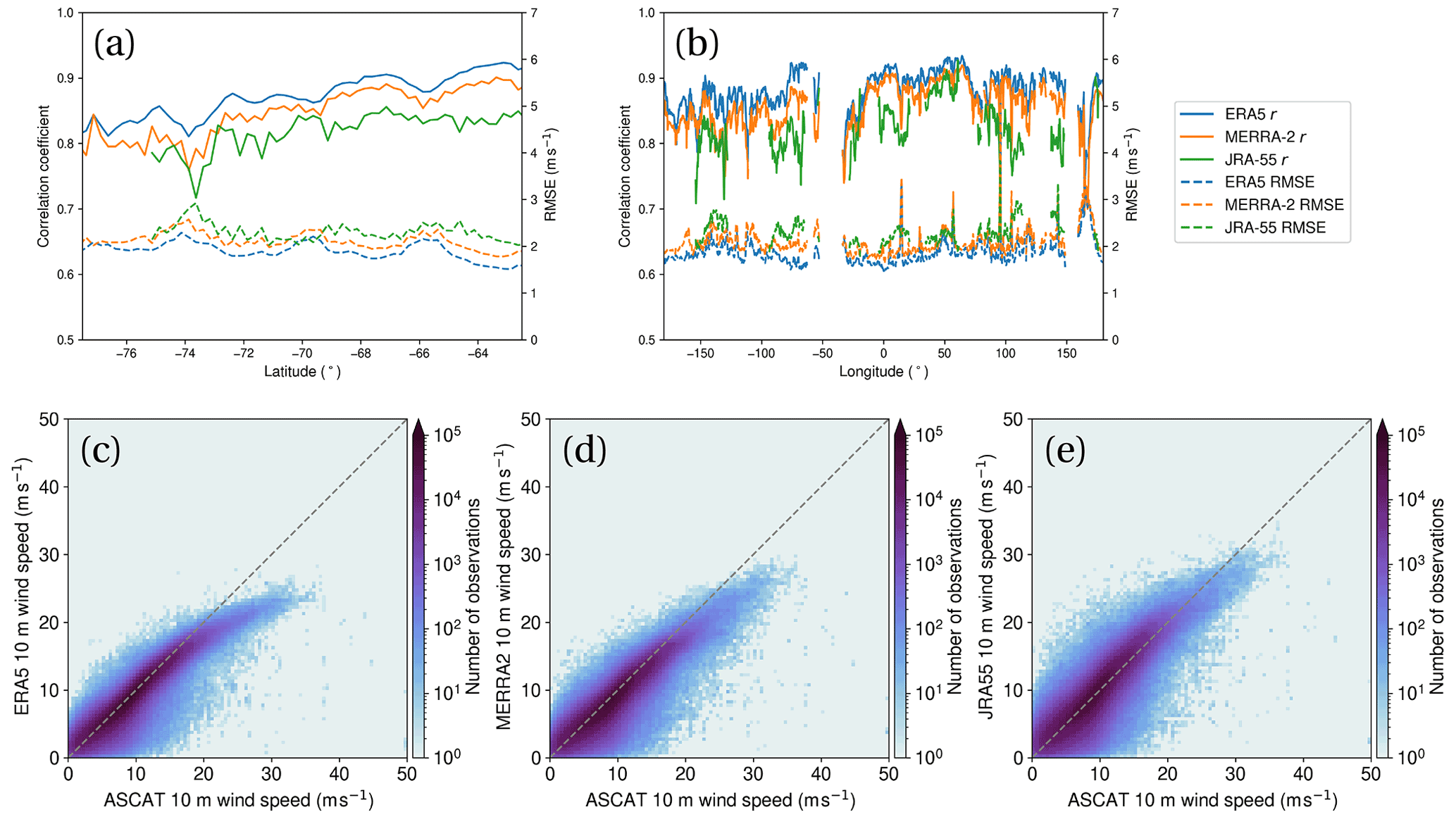
Figure 3Mean wind speed performance metrics by (a) latitude and (b) longitude against ASCAT for ERA5 (blue), MERRA-2 (orange) and JRA-55 (green). Includes correlation coefficient (solid) and RMSE (dashed). (c–e) Heat map scatterplots of collocated data points within the coastal easterly domain for (c) ERA5, (d) MERRA-2 and (e) JRA-55. Only data points collocated in all three reanalyses are included in panels (c)–(e). Data points which are rain flagged or have a GMF-matchup flag value over 2 are not included.
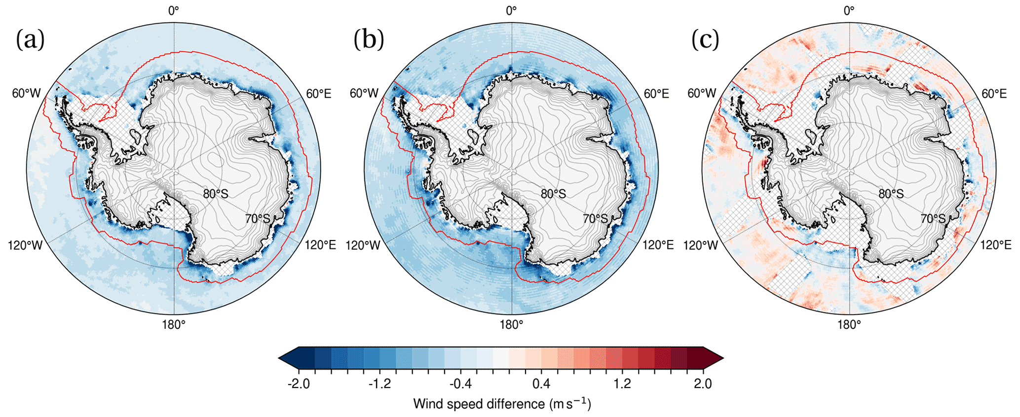
Figure 4Mean reanalysis minus ASCAT 10 m wind speed for the period 2010–2017 for (a) ERA5, (b) MERRA-2 and (c) JRA-55. Hourly data are used for ERA5 and MERRA-2 with 6-hourly from JRA-55. Data points which are rain flagged or have a GMF-matchup flag value over 2 are not included and pixels with fewer than 50 ASCAT-reanalysis collocations are masked (hatched region). Orography at 300 m intervals (from the ERA5 invariant fields) is marked with grey contours. The region within the red contour is the coastal easterlies domain, identified where either the ERA5 2010–2017 mean zonal wind is less than zero or the location is within a 12-grid box buffer drawn from the coast.
Values of the ASCAT-reanalysis Pearson correlation coefficient within the coastal easterly domain are highest in ERA5 at 0.91, but MERRA-2 and JRA-55 near-surface winds are also closely correlated with ASCAT at 0.89 and 0.85, respectively. Latitude–mean correlation coefficients are highest in ERA5 at all longitudes (Fig. 3b) but longitudinal variations in performance are very similar between reanalyses. Correlation coefficients decline and RMSE increases with increasing proximity to the coast itself (i.e. higher southern latitudes) (Fig. 3a). Scatterplots (Fig. 3c–e) indicate a high density of points clustered close to the 1:1 line (dashed grey) between 0 and 20 m s−1 though JRA-55 exhibits a higher spread of overestimated wind speeds. All three reanalyses exhibit a tendency towards negative bias with respect to ASCAT at high wind speeds (above 20 m s−1). This may in part relate to the localised and short-term nature of extreme winds observed with the scatterometer. It is also possible that the representation of extremes is affected by the assimilation method; for example, the assimilation of extreme scatterometer winds into ECMWF analyses is sensitive to the data thinning and quality control procedures (De Chiara et al., 2017). Underestimation of high wind speeds is also a characteristic of ERA-Interim when compared with in situ wave glider wind observations from the sub-Antarctic Southern Ocean by Schmidt et al. (2017). The mean bias across the coastal easterly domain for ERA5, MERRA-2 and JRA-55 is −0.51, −0.72 and −0.06 m s−1, respectively, but sampling only wind speeds above 20 m s−1 this bias changes by −3.89, −3.88 and −1.54 m s−1 (i.e. becomes more negative). For reference, on average across all the 10 m surface station wind speed data from Mawson, Neumayer and Dumont d'Urville (the better exposed sites), this change in the bias induced by sampling only wind speeds above 20 m s−1 would be −4.65, −5.13 and −4.53 m s−1, respectively.
Maps of the reanalysis bias with respect to ASCAT (Fig. 4) indicate that the largest differences between the reanalyses and observations are found in the near-coastal region. Both ERA5 and MERRA-2 exhibit a band of negatively biased wind speeds close to the coastal margins. Note that regions of missing data in JRA-55 are where not enough points could be collocated (i.e. fewer than 50) between ASCAT and the reanalysis due to the reduced frequency (6-hourly) of data compared to ERA5 and MERRA-2 (hourly). Some regions of elevated bias are found close to complex or steep orography. For example, ERA5 and MERRA-2 exhibit stronger negative biases along Enderby Land at 50–55∘ E, a site identified by Sampe and Xie (2007) as a likely hotspot of orographically-driven winds. The western Antarctic Peninsula (west of 60∘ W) is a region of underestimated wind speeds in all three reanalyses, and underestimation of winds north of the Ross Ice Shelf along the Transantarctic Mountains (from about 65–75∘ S and 170∘ E) is found in ERA5 and MERRA-2. JRA-55 does not have as consistent a sign of difference in wind speed compared to the other two reanalyses, but some similar patterns emerge, including more pronounced bias close to the east Antarctic coast and along the western peninsula. Near-coastal negative wind speed biases increase in ERA5 and MERRA-2 from January to March (Figs. S2 and S3a–c in the Supplement) as wind speeds over the region increase (Fig. S1a–c).
It is interesting to note that although the selected domain has an overall easterly low-level wind regime, biases in the zonal and meridional components of ERA5, MERRA-2 and JRA-55 10 m winds are mixed around the coast (Fig. S5). The offshore easterly sector has much lower mean directional constancy than the onshore sector (van den Broeke and van Lipzig, 2003) meaning near-surface wind directions are more variable. As a result, biases may cancel out to an extent when individual wind components are calculated if the reanalysis bias is insensitive to wind direction.
Our analysis agrees with that of Carvalho (2019) who shows increasing reanalysis errors with respect to satellite wind products near the poles. Carvalho (2019) also finds that MERRA-2 generally outperforms JRA-55, CFSR, JRA-55 and ERA-Interim winds at high southern latitudes. We find that the more recent ERA5 now slightly outperforms MERRA-2 in the coastal region, consistent with the findings of Belmonte Rivas and Stoffelen (2019) who report an improvement in ERA5 ocean winds relative to ERA-Interim.
Some of the observed differences between ASCAT and the reanalyses may be due to inconsistencies in how scatterometer and reanalysis 10 m winds are derived, although the effects of atmospheric stability are accounted for in our analysis by making use of the reanalysis neutral winds rather than stability-dependent winds. One possible remaining issue is mismatches in the designation of open ocean and sea ice in the reanalysis and scatterometer datasets; some regions of non-zero ERA5 sea ice concentrations were found within the collocated ASCAT fields. Excessively smooth sea ice distributions in the marginal ice zone have been linked to increased wind speed RMSE with respect to aircraft observations at high northern latitudes (Renfrew et al., 2021). To estimate the effect of mismatched sea ice, the evaluation of ERA5 was recalculated with the regions of non-zero ERA5 sea ice concentration masked out. With this masking applied, the overall mean bias in coastal easterly domain was reduced from −0.67 to −0.59 m s−1 with some error-prone regions around the edge of the ice pack removed (not shown), but the correlation coefficient only increased from 0.91 to 0.92.
Ocean currents may also have an effect on the results as ASCAT measures surface wind stress relative to a moving surface, but within the region of the easterlies this effect is expected to be small with an estimated mean surface speed south of 65∘ S for the 2010–2017 period of 0.007 m s−1 from the OSCAR Surface Currents dataset (ESR, 2009). The analysis of Belmonte Rivas and Stoffelen (2019) includes a correction for ocean currents which reduces a positive zonal wind bias north of the coastal easterly domain in the Southern Ocean (i.e. too strong westerlies) in ERA5, with the magnitude of the effect around 0.1 m s−1 (see Fig. 10 therein). The effects of air density differences on the estimation of neutral winds are also expected to have a small impact on the results. Accounting for this could reduce reanalysis biases by about 0.1 m s−1 in the near-coastal region based upon the analysis of de Kloe et al. (2017) (see Fig. 13). In summary, these sources of inconsistency do have a small impact but are not able to explain large wind speed biases exceeding 2 m s−1 such as those found close to complex Antarctic orography.
3.2 State-dependent performance against station measurements: SOM regimes
3.2.1 Composited synoptic and katabatic conditions
Coastal stations are exposed to a variety of synoptic and mesoscale flow regimes, with the largest short-term variability in winds observed offshore (Fig. 1). SOM nodes for each station organise broadly into states for which the pressure gradient is more intense and ones where it is reduced (Fig. 5 and Table S1 in the Supplement). However, the SOM nodes are not a simple continuum between those two extremes; a number of nodes represent the varied orientation of synoptic pressure gradients relative to the location of the station. For example, at Dumont d'Urville (Fig. 5b), nodes (1,1) and (1,2) have comparable large-scale pressure gradients but the low-level pressure contours associated with the offshore low are orientated along the coast for (1,1) whereas in (1,2) they are oriented more perpendicular to the coast. This is due to the differing position of the low pressure centre with respect to the station. The strongest 10 m wind speeds near each station are observed during states with the largest synoptic pressure gradient ((1,2) at Casey, (1,1) at Mawson and Neumayer and both at DDU). The maximum in wind speed is generally found onshore, which could be an indication of combined katabatic and synoptic forcing (e.g. Turner et al., 2009; Orr et al., 2014) but is also the region of maximum large-scale pressure gradient force on average (van den Broeke and van Lipzig, 2003).
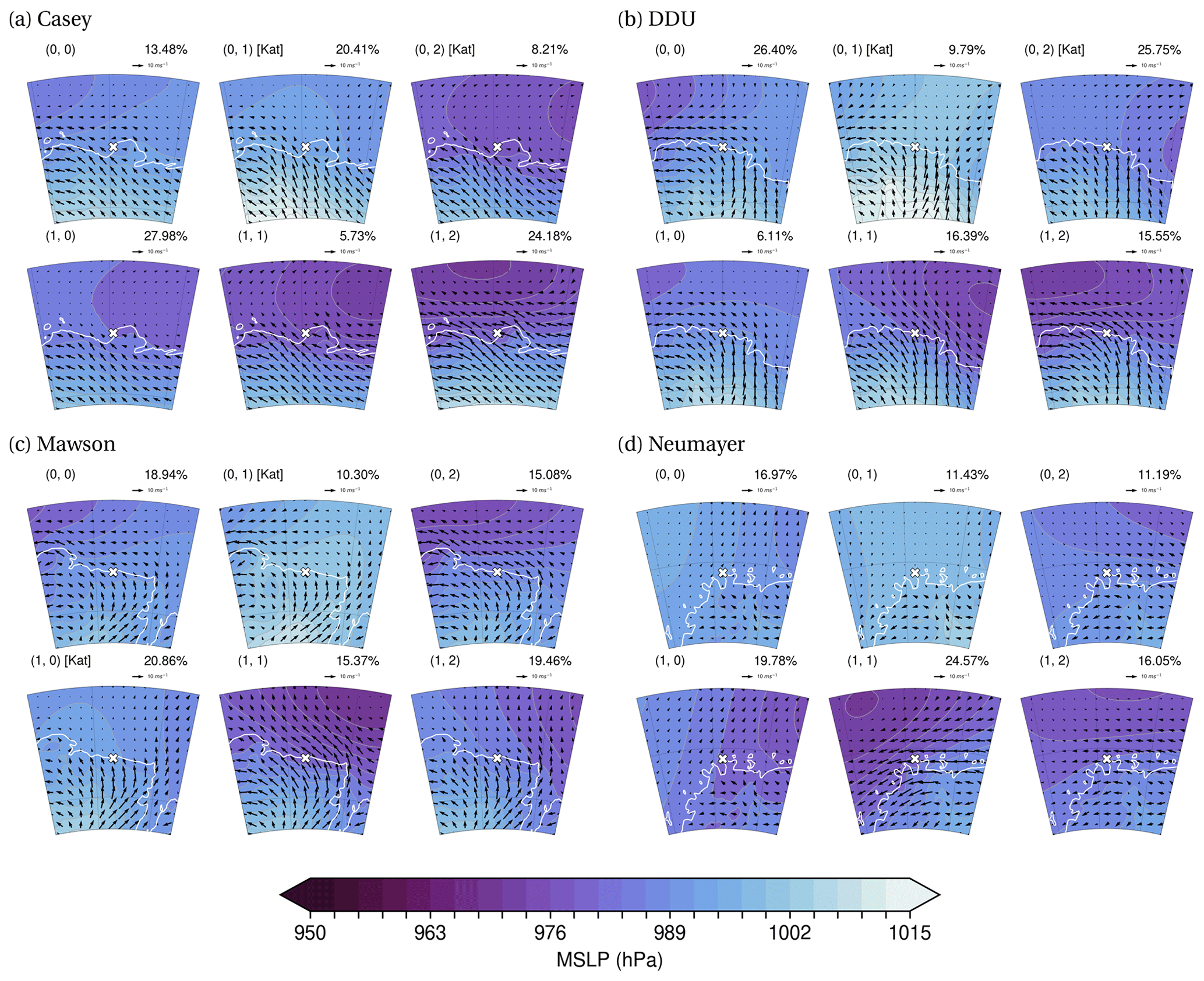
Figure 5Composited ERA5 mean sea-level pressure (MSLP) with 10 m wind vectors for each node at (a) Casey, (b) DDU, (c) Mawson and (d) Neumayer from SOMs calculated for the period 2010–2017. Station locations are marked as a white cross. Nodes with limited synoptic forcing but favourable conditions for katabatic forcing are labelled with a [Kat].
Each station has two or three nodes which correspond to reduced pressure gradients (Table S1), including one with high pressure onshore (node (0,1) in Fig. 5). To assess the likely contribution of katabatic flow to these states, the acceleration term due to katabatic forcing K (KAT index, hereafter) is calculated for each ERA5 grid point following the approach described in van den Broeke and van Lipzig (2003). Our implementation of this approach is detailed in Appendix C.
Composites of the katabatic index (Fig. 6) reveal that the exposure to conditions favouring katabatic forcing varies considerably between stations. The highest index values are observed to the east of Dumont d'Urville, where the nearby steep coastal slopes favour considerable local baroclinicity. For all stations, the largest nearby composited KAT index values are for node (0,1), i.e. during high pressure conditions. These nodes are also associated with the lowest mean total cloud cover in ERA5 (not shown), favouring long-wave cooling and a stable boundary layer, and exhibit a sharp cutoff in wind speeds at the coast. Nodes which exhibit these signs of strong katabatic influence but little synoptic influence (i.e. a low background pressure gradient) will be referenced several times in the reanalysis evaluation, so to help quickly identify them they have been marked with a “[Kat]” in Figs. 5 to 10. However, these are subjectively classified and large-scale synoptic forcing in other nodes, for instance due to offshore cyclones, does not preclude the continued occurrence of katabatic winds, hence SOM states other than those marked with a “[Kat]” are still likely to contain a katabatic influence.
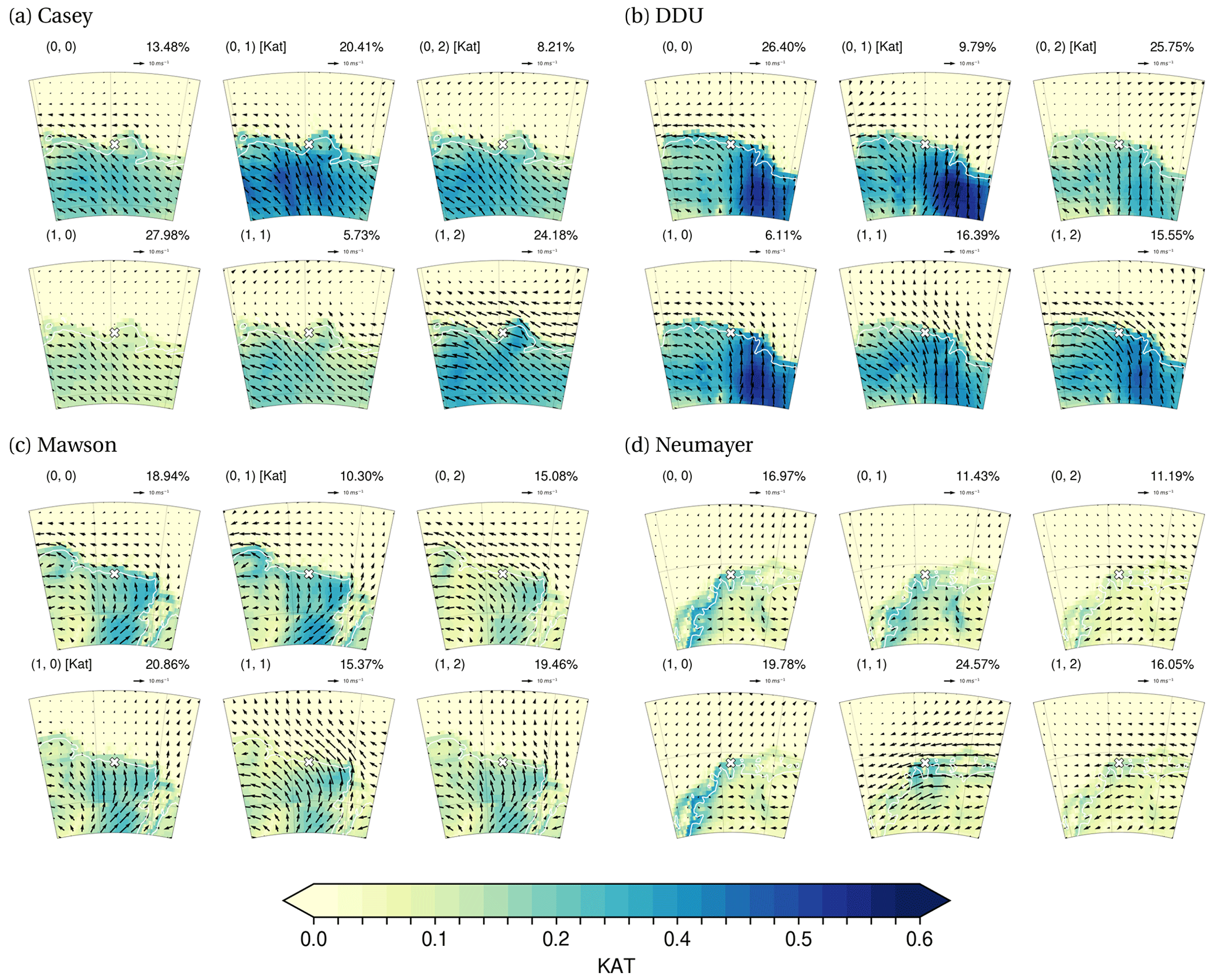
Figure 6Composited ERA5 katabatic acceleration term with 10 m wind vectors overlain for each node at (a) Casey, (b) DDU, (c) Mawson and (d) Neumayer from SOMs calculated for the period 2010–2017. Station locations are marked as a white cross. Nodes with limited synoptic forcing but favourable conditions for katabatic forcing are labelled with a [Kat].
3.2.2 Performance at Casey station
With the lowest Pearson correlation coefficient (r) across reanalyses, near-surface winds observed at Casey station are poorly represented (Fig. 7), especially in JRA-55 and MERRA-2 in which the topography of the Law Dome is highly smoothed (Fig. 2). Large differences in both the zonal and meridional wind components between observations and reanalysis occur at Casey (Fig. 7 profiles). One standout is node (1,2), a state in which the pressure contours are aligned to favour some flow around the Law Dome. r values for node (1,2) are higher than for other nodes (Table D1a), largely due to better representation of wind speed variability above 15 m s−1. In JRA-55, for instance, there is considerable overestimation of near-surface wind speeds below 10 m s−1 (Fig. 7i) and large spread where the orographic flow blocking is unrepresented, shifting abruptly to consistent underestimation but improved correlation above 10–15 m s−1. This large negative bias at elevated wind speeds is present in the other two reanalyses and is in fact greatest in ERA5 (Fig. 7c).
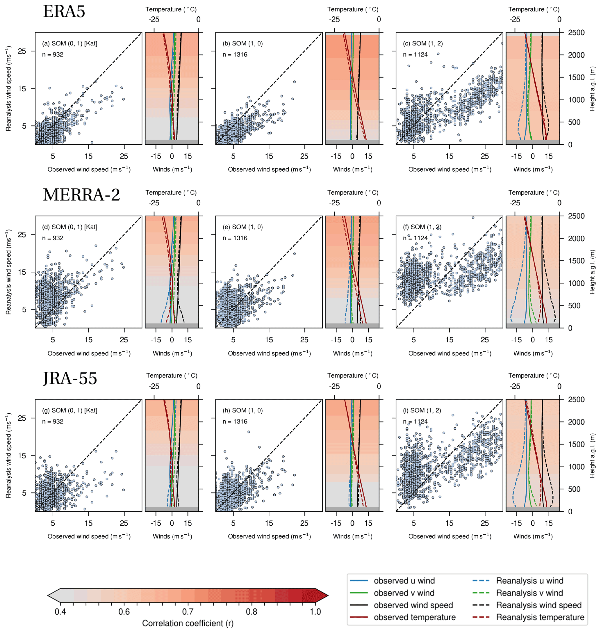
Figure 7Reanalysis–observation wind intercomparison by SOM node at Casey for (a–f) ERA5, (g–l) MERRA-2 and (m–r) JRA-55 for the period 2010–2017. The three most frequently occurring nodes (accounting for 72.6 % of the total variability) are shown, with the full set in Sect. S4. For each node the following is plotted: (left) scatterplots of observed vs. reanalysis 10 m wind speeds and (right) vertical profiles of mean wind speed (black), u wind (blue), and v wind (green) and temperature (red) from observations (solid) and reanalysis (dashed). Shading in the background of each profile indicates the correlation coefficient between observed and reanalysis wind speed at that level. Nodes with limited synoptic forcing but favourable conditions for katabatic forcing are labelled with a [Kat]. All shaded correlation coefficients are significant at the 99 % level, according to a two-sided t test.
Reanalysis wind profiles at Casey (Fig. 7, profiles) exhibit an excessively strong and deep easterly (negative u) jet at 300–400 m height above ground level (a.g.l.) which is absent in the observations and particularly pronounced when a large-scale pressure gradient is present and oriented to allow flow around the Law Dome (node (1,2)). This bias is largest in MERRA-2. Wind speed correlation coefficients improve with height across most nodes. Temperature profiles in the lowest 1000 m are most realistic in ERA5 and are generally biased low in MERRA-2 and JRA-55, especially for the strong synoptic forcing node (1,2). The temperature profile observed at Casey is often characterised by a near-surface inversion layer in the lowest 100–200 m (see Fig. S10) topped by a constant lapse rate which may not be well captured in the coarser products.
3.2.3 Performance at Dumont D'Urville station
At Dumont d'Urville (DDU), 10 m reanalysis winds are more closely aligned with observations than at Casey but performance characteristics vary considerably by SOM state (Fig. 8 scatterplots). ERA5 has a systematic negative bias at high wind speeds (Fig. 8a and c). By contrast, MERRA-2 and JRA-55 exhibit quite distinct performance regimes at high wind speeds, which can be seen by comparing node (0,0) and (1,1) for the two reanalyses. These reanalyses consistently overestimate wind speeds when the pressure contours favour a more northerly flow (node (0,0)) but underestimate it when the observed low-level flow has a stronger southerly component (node (1,1)). Root mean square error (RMSE) is also slightly higher for all reanalyses in node (1,1) compared to node (0,0) (Table D1b).
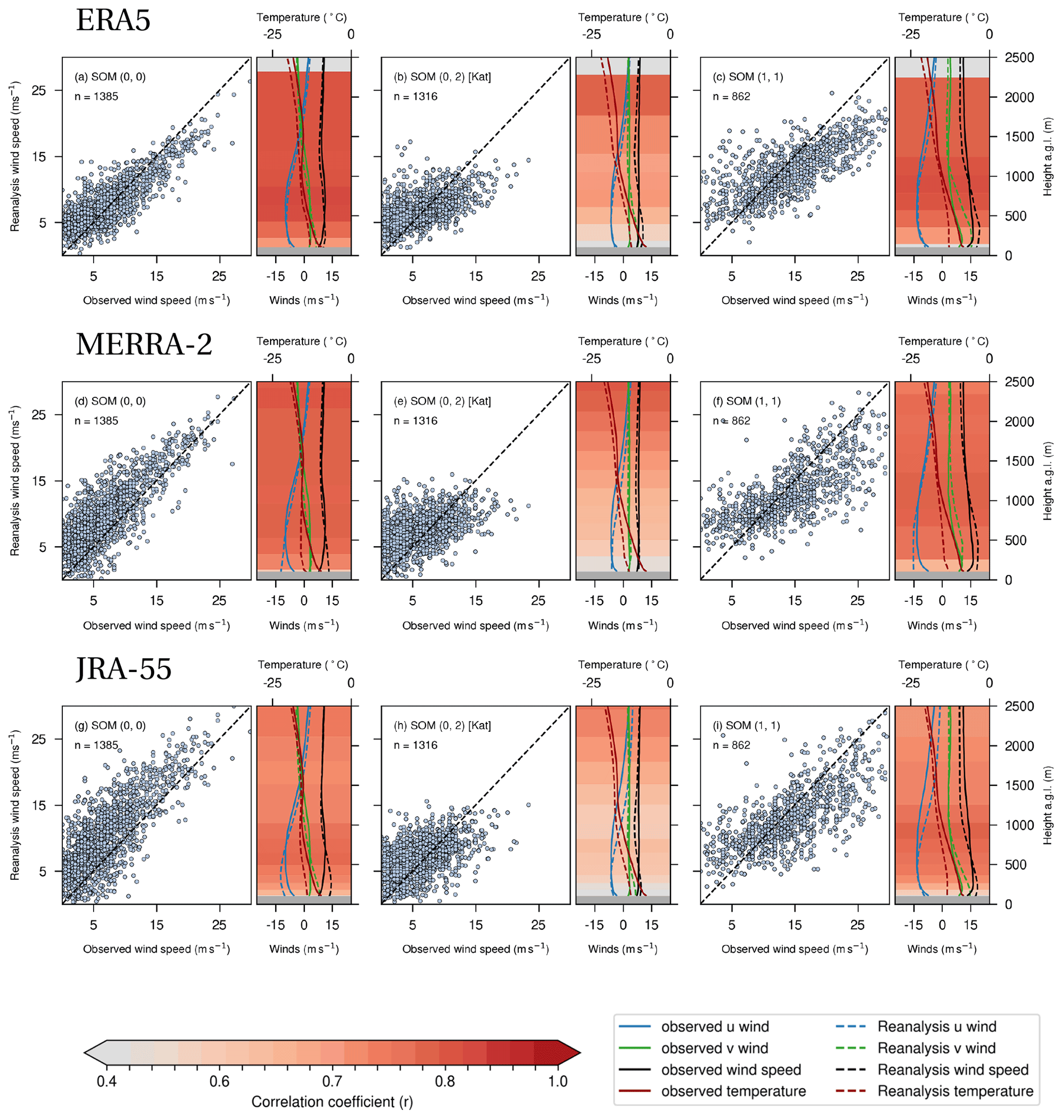
Figure 8As in Fig. 7 but for DDU. All shaded correlation coefficients are significant at the 99 % level, according to a two-sided t test. These three SOM nodes account for 68.5 % of the total variability at DDU.
The displayed state which favours katabatic forcing ((0,2)) is characterised by a reduced interquartile range (IQR) with respect to the observations in all three reanalyses (Table D1b), resulting in overestimated low wind speeds and underestimated high wind speeds. Correlation coefficients (r) are also reduced for this state, in part due to the smaller range of wind speeds. As with Casey, r values are consistently highest in ERA5 across nodes.
Observed DDU wind profiles exhibit a deep easterly jet accompanied by a shallower southerly layer, both of which are strongest in node (1,1) and (1,2) when the synoptic pressure gradient is highest (Fig. 8c, f, i). Correlation coefficients in the lowest 2500 m are higher at DDU compared to Casey, consistent with near-surface wind data. The core of the easterly winds in jet regimes is similar to observations in all three reanalyses (Fig. 8 nodes (1,1)), with the main difference between reanalyses being in the height of the jet. The observed jet during the strongest synoptic forcing in node (1,1) is a deep but uniform feature between 200 and 1000 m a.g.l. whereas the reanalyses represent it with greater shear above and below a jet core. The jet structure appears to be more realistic in ERA5 for the katabatic (0,2) state compared to MERRA-2 and JRA-55 which position the core of the easterlies several hundred metres too close to the surface and subsequently have considerably lower r values in the lowest 1000 m compared to other nodes. The structure of the meridional winds at DDU is a point of disagreement between reanalyses; in ERA5 the southerly layer is deep and excessively strong in the jet case (Fig. 8c) whereas in JRA-55 the structure is realistic but the southerlies are too consistently strong (Fig. 8i).
Compared to Casey, a more complex temperature profile is observed at DDU. Although not clear from the averaged temperature profiles, near-surface inversions are again common (Fig. S10) but they are also accompanied by inversions at altitudes above 1000 m a.g.l., generating a distinct reverse S shape in the temperature profile which is present in reanalyses but is smoothed and varies considerably in vertical structure between dataset. Substantial negative temperature biases occur in the lowest 1000 m in JRA-55 and MERRA-2, reaching 5 K at 100 m a.g.l.
3.2.4 Performance at Mawson station
Compared to other stations, performance statistics differ little between reanalyses at Mawson (Fig. 9), though as before ERA5 has marginally higher r in all nodes. All three underestimate the highest wind speeds, for example in node (0,0) (Fig. 9a, d, g). This underestimation of elevated wind speeds at Mawson is also a feature of the Met Office Unified Model (UM) which was not rectified by switching to a very high horizontal or vertical grid resolution (Orr et al., 2014).
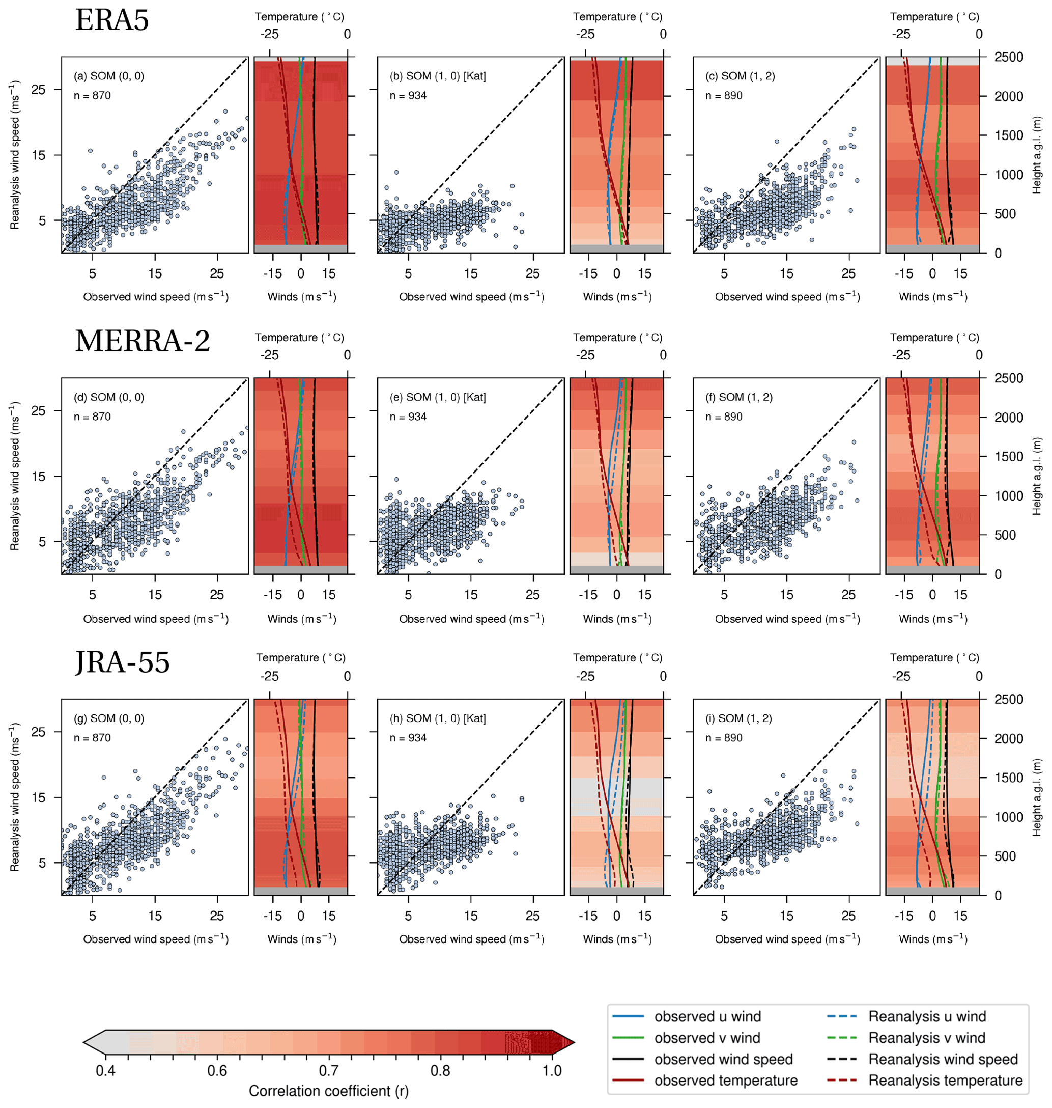
Figure 9As in Fig. 7 but for Mawson. All shaded correlation coefficients are significant at the 99 % level, according to a two-sided t test. These three SOM nodes account for 59.3 % of the total variability at Mawson.
As at DDU, the katabatic state shown for Mawson ((1,0)) is characterised by a considerably reduced IQR of reanalysis wind speeds with respect to observations (Table D1c); when an intense pressure gradient is absent, reanalyses appear to fall into a regime of underestimating the large local wind speed variability. One interpretation is that there are two distinct flow regimes at Mawson. If the large-scale pressure gradient is strong enough, the onshore and offshore wind field become continuous, whereas when it is weaker terrestrial (likely katabatic) winds are cut off abruptly at the coast, and the representation of the winds becomes sensitive to the placement and turbulent characteristics of the katabatic jump.
The easterly jet at Mawson is similar to DDU (Fig. 9). As with DDU, correlation coefficients against vertical wind measurements vary by SOM node at Mawson. Interestingly, high and consistent r values are found throughout the 2500 m profile for each of the three reanalyses in node (0,0) during which the pressure gradient is high but the southerly layer is shallow as a result of the orientation of the low pressure centre offshore, directing geostrophic flow of maritime origin towards Mawson station.
The temperature profile at Mawson is comparable to DDU in its reverse S shape. Again, this is a feature that varies greatly between reanalyses; the structure is most realistic in JRA-55 and ERA5. This may explain why the jet structure (with an elevated easterly core and lower southerly core) is also more realistic in those reanalyses compared to MERRA-2 for which this structure in the vertical wind profile is not seen. As with other stations, JRA-55 and MERRA-2 exhibit a cold bias in the lowest 1000 m, with that of JRA-55 equalling or exceeding 5 K at the surface.
3.2.5 Performance at Neumayer station
As described in Sect. 2.3.1, Neumayer has quite different local terrain characteristics compared to other stations, being situated on a flat ice shelf with comparably small orographic height differences between reanalyses and reality. Near-surface wind disagreements are much smaller at Neumayer than at the other stations considered here (Fig. 10). As a result, the lowest mean RMSE values are found here (Table D1d). ERA5 appears to be the best performing reanalysis by a larger margin than at Mawson. By contrast, lower r values and higher RMSE are found for all SOM nodes in JRA-55 (Table D1d). There is little discernible difference in the scatterplot characteristics between SOM nodes at Neumayer.
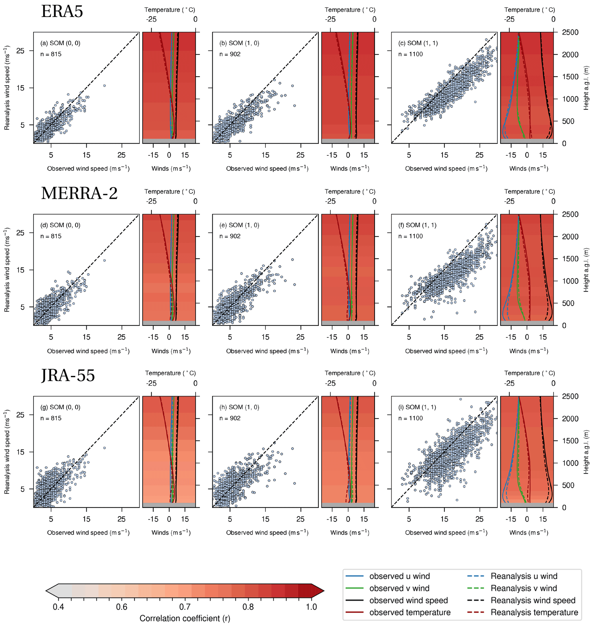
Figure 10As in Fig. 7 but for Neumayer. All shaded correlation coefficients are significant at the 99 % level, according to a two-sided t test. These three SOM nodes account for 61.3 % of the total variability at Neumayer.
Consistent with better reanalysis performance against surface station winds, both reanalysis wind profiles and reanalysis temperature profiles (Fig. 10) compare relatively favourably with Neumayer upper air data. ERA5 and MERRA-2 stand out here with consistently high wind speed r values across SOM nodes while JRA-55 exhibits some degradation in fidelity in the lowest 500 m, especially for nodes (0,2) and (1,2) (Fig. S9o and r), both of which are subject to low-level flow passing over the complex coastal terrain east of Neumayer. The jet structure is well represented, including a shallow southerly flow. However, the core of the easterly jet, seen most clearly in node (1,1), is consistently underestimated by all three datasets. Baroclinicity and the coastal slopes nearby are thought to introduce ageostrophic motions at Neumayer (Kottmeier, 1986; Klöwer et al., 2014) though the katabatic pressure gradient force is not as large over the ice shelf as further inland (van den Broeke and van Lipzig, 2003). Gorodetskaya et al. (2020) show that a slight negative ERA5 wind speed bias is also a characteristic of low-level jets occurring in atmospheric river conditions at Neumayer; our analysis indicates that this bias applies more generally to strong wind conditions, for example as in node (1,1).
In this paper, we have evaluated the representation of Antarctic coastal winds in three current reanalyses. The analysis aims to quantify representation of the mean state and short-term variability of coastal winds, making use of the few observational datasets available within the coastal easterly domain. There is a great deal in common between reanalyses in the representation of time–mean coastal winds and their variability. These similarities and the differences which do exist point to some critical processes which are important for representation of the coastal winds.
Firstly, the representation of orography is especially important at the coast and has a large impact on reanalysis performance. As shown in Sect. 2.3.1, the slope of the coastal orography in reanalyses is smoothed, leading to large differences in surface height at the latitudes of most coastal stations, with the exception of Neumayer where the local terrain is flat. At Casey, the reanalysis performance is poor across the board, especially for the coarser MERRA-2 and JRA-55, suggesting the local orography (in particular the Law Dome) has a large effect on the winds, including those well above the surface layer. Whereas reanalysis winds are quite realistic at Neumayer, correlation coefficients only improve at Casey when the large-scale flow is relatively unimpeded by the Law Dome. The comparison with ASCAT also points to a critical role for orography in the coastal margins; reanalysis performance with respect to ASCAT declines with increasing proximity to the coast, and biases are especially large close to complex orography such as the Transantarctic Mountains, Law Dome and around Enderby Land. Orographic processes such as barrier and tip jet formation are likely to be important in the Antarctic coastal margins and sources of marine wind speed biases in reanalyses.
A second and related theme is the difficulty in characterising low-wind states dominated by katabatic forcing when a strong large-scale synoptic pressure gradient is absent (nodes marked with a “[Kat]” in Figs. 7, 8 and 9). This is clearest at DDU and Mawson which are subject to semi-permanent katabatic winds. Vignon et al. (2019) show how a typical feature of ERA-Interim and ERA5 is an underestimated range between the 5th and 95th percentiles of wind speed in the lowest 200–300 m. Our analysis indicates this effect may be greatly enhanced during these [Kat] states; at DDU this mostly appears as an overestimate of low wind speeds whereas at Mawson high wind speeds are underestimated. The exact source of this misrepresentation is not clear from this analysis but the implication is that winds in the coastal margins are more variable than reanalyses suggest. A caveat of this analysis is that katabatic winds are a highly terrain-dependent and locally variable phenomenon at the coast; the sign of the bias is quite sensitive to the collocation. Furthermore, the contribution of momentum from katabatic flow to maritime winds responsible for coastal currents remains unquantified, but our analysis indicates that katabatic regimes may be a substantial source of model error.
A third point of interest is that temperature profiles at coastal stations differ between reanalyses, and although this research focuses on winds, these differences could be important for the baroclinic conditions which influence coastal winds. A realistic zonal jet feature does occur in the lowest 1500 m in reanalyses during states with strong synoptic forcing (except at Casey where it is greatly overestimated), but MERRA-2 and JRA-55 exhibit substantial cold biases in approximately the lowest 1000–1500 m. A MERRA-2 cold bias in both East and West Antarctica was also found when compared with observations from the 2010 Concordiasi field campaign (Ganeshan and Yang, 2019) and against coastal surface stations (Jones et al., 2016; Gossart et al., 2019). Reduced wind speed correlation coefficients at height, especially in MERRA-2 and JRA-55 during low-wind katabatic states, may be in part related to these temperature biases and in part to the representation of temperature inversions. A dual inversion structure as shown for Mawson and DDU in Fig. S10 is common for the Antarctic coastline (Truong et al., 2020) and poses a challenge for faithful representation of near-coastal thermodynamic profiles, but its role in the representation of wind profiles warrants further investigation.
Implications for use of reanalysis datasets
Reanalyses are capable of representing important features of the coastal wind field and its variability, including the existence of a jet feature peaking during strong synoptic forcing. Many of the differences against observations are consistent between datasets, including underestimated near-surface winds above 20 m s−1, underestimated interquartile range in states with reduced pressure gradients where katabatic winds dominate, poor representation at Casey where a local orographic feature plays a major role, and improved performance at Neumayer over relatively flat surface conditions.
Alongside the detailed breakdown of performance statistics across various metrics, rankings for each reanalysis by station and by metric (using only surface wind speed) are given in Appendix D. These indicate that ERA5 exhibits the best performance overall, especially for r (as with ASCAT). Higher resolution in ERA5 also supports more realistic coastal orography; steeper coastal slopes are in turn likely to be important for realistic terrain-driven baroclinicity and katabatic forcing (Fulton et al., 2017). Temperature profiles also appear to be most realistic in ERA5, with JRA-55 and MERRA-2 exhibiting substantial cold biases in the lowest 1000 m a.g.l. and a decline in wind speed r values near the top of the easterly jet region in some SOM states. However, JRA-55 and MERRA-2 exhibit lower mean bias and bias in interquartile range. Negative bias is especially large at high wind speeds in ERA5 when compared with both station measurements and ASCAT. The contribution of this substantial and time-varying bias to long-term trends and wind stress in the coastal sector warrants further investigation but these results suggest that using ERA5 to analyse coastal extremes requires careful consideration of the effect that a systematic negative bias could have upon the results.
ASCAT observations and sonde data were assimilated into all three reanalyses, meaning only the 10 m wind observations are quasi-independent in our evaluation. The assimilated observations were likely important for reanalysis performance and so further evaluation with unassimilated observations would be valuable. For example, the effect of assimilating new Antarctic dropsonde observations from the Concordiasi field experiment on ECMWF forecasts was found to be larger away from the coastal regions where most of the existing radiosondes are launched (Boullot et al., 2016) and additional sonde observations from the Year of Polar Prediction improved wind speed forecasts over West Antarctica (Bromwich et al., 2022).
The representation of winds within the region of the Antarctic coastal easterlies in the ERA5, MERRA-2 and JRA-55 reanalyses has been evaluated by comparison with in situ and satellite observations, including summertime ASCAT observations over the marine sector and observations from four coastal stations. For each station, the sensitivity of reanalysis performance to changes in the driving flow regime was analysed using SOMs derived from ERA5 MSLP fields.
A comparison with ASCAT scatterometer winds shows that wind speed variability within the region of the coastal easterlies is well represented by the reanalyses, with correlation coefficients of 0.91 in ERA5, 0.89 in MERRA-2 and 0.85 in JRA-55. Generally, near-surface wind speeds offshore are biased slightly low across the whole coastal easterly sector in ERA5 and MERRA-2 whereas JRA-55 biases are closer to zero on average but have large local variations. Correlation coefficients decrease with proximity to the coast and the ASCAT fields reveal near-coastal wind features (especially close to complex orography) whose magnitude is not well captured by the reanalyses. All three reanalyses exhibit larger negative biases relative to scatterometer data at wind speeds exceeding 20 m s−1.
Reanalysis performance against observations is much more sensitive to different flow regimes (characterised with SOMs) at coastal slope stations (in particular Mawson and DDU) than over the flatter terrain of Neumayer. Time series correlation coefficients (r) between both surface and upper air wind speeds and collocated reanalysis wind speeds are consistently higher in states with strong synoptic forcing and especially when low-level flow is directed onshore. By contrast, r values consistently drop for states with limited synoptic forcing but favourable conditions for katabatic forcing. This is in part due to the lower wind speeds but also because the reanalyses' interquartile range is lower than observations at both Mawson and DDU during those states. Performance against observations from Casey is poor due to the effect of the Law Dome on the low-level flow. Representation of orography is likely critical to variations in reanalysis fidelity by state and station. MERRA-2 and JRA-55 have large cold biases in the lowest 1500 m which may be important for the realism of low-level coastal winds.
Overall, ERA5 has the highest near-surface wind r values compared to both station measurements and ASCAT over the coastal easterly sector. High r values are generally mirrored by low RMSE. A more realistic temperature profile, better characterisation of variability and more faithful representation of orography gives greater confidence in ERA5 as a benchmark dataset for Antarctic coastal winds. It should be emphasised, however, that performance is similar between reanalyses and many key deficiencies are shared, including relatively large biases against ASCAT near the coast and at high wind speeds, poor performance close to the Law Dome and underestimation of the wind speed variability when synoptic forcing is reduced, and katabatic forcing is important.
These results shed light on some of the challenges associated with evaluating model-based datasets in the Antarctic coastal region and underscore the role of orography. Furthermore, they demonstrate the usefulness of an evaluation approach designed to interrogate reanalysis or model performance under varied atmospheric states, given the high variability of the coastal sector. This SOM-based methodology offers an approach to reanalysis evaluation that is process-oriented and could be applied to other reconstruction datasets or assessment of climate models. In future work the insights from this analysis will be used to guide regional model sensitivity experiments and to help constrain future projections of the coastal easterlies in coupled climate models.
For the comparison with station measurements, all results were recalculated after shifting the collocated reanalysis grid point one point to the north and south.
Although this shift causes a slight degradation in correlation coefficients for all reanalyses, stations and SOM nodes, the main results reported in Sect. 3.2.2 to 3.2.5 are robust, except for a large impact upon the value of the bias for wind speeds below 10 m s−1 in states and at stations where the synoptic forcing is reduced but katabatic forcing is favoured. Low-wind states in steep-slope coastal regions therefore appear to be highly sensitive to collocation. For example, in ERA5 for SOM node (0,2) at DDU the bias is 0.77 m s−1, but shifting the collocated point south increases this to a 5.19 m s−1 bias (with a similar effect on low winds in other states) and, conversely, shifting it north gives a −0.9 m s−1 bias. Large wind speed gradients occur at the Antarctic coast, especially during katabatic-dominated states, meaning winds upslope (south) of surface stations may be much stronger than those just offshore (north). Estimates of reanalysis or model bias in the representation of katabatic winds based upon point collocation with coastal station measurements should therefore be treated with caution. Our focus is primarily upon differences between nodes, stations and reanalyses.
A variety of SOM configurations were tested (Fig. B1). Node correlation and pair correlation were calculated based on the approach of Gibson et al. (2017). Node correlation is defined as the mean correlation between the data points comprising individual SOM nodes and the data points of timesteps to which they were assigned (i.e. a reanalysis timestep is assigned to a SOM node based on the mean squared difference, and then the correlation is calculated between all data points in that timestep and all data points in the SOM node). The pair correlation is defined as the mean correlation between all possible pairs of SOM nodes. The node correlation is therefore intended as a measure of how realistic SOM nodes are (larger values are desirable) whereas pair correlation is a measure of how similar they are to each other (lower values are desirable). It should be noted that pair correlations near one for configurations with few nodes are a result of the background large-scale conditions of the Antarctic; high pressure over the continent and low pressure offshore within the circumpolar trough, with this dipole not differing greatly between nodes in Fig. 5 despite varying patterns. Only at Neumayer is there some evidence in Fig. 5 of this dipole reversing.
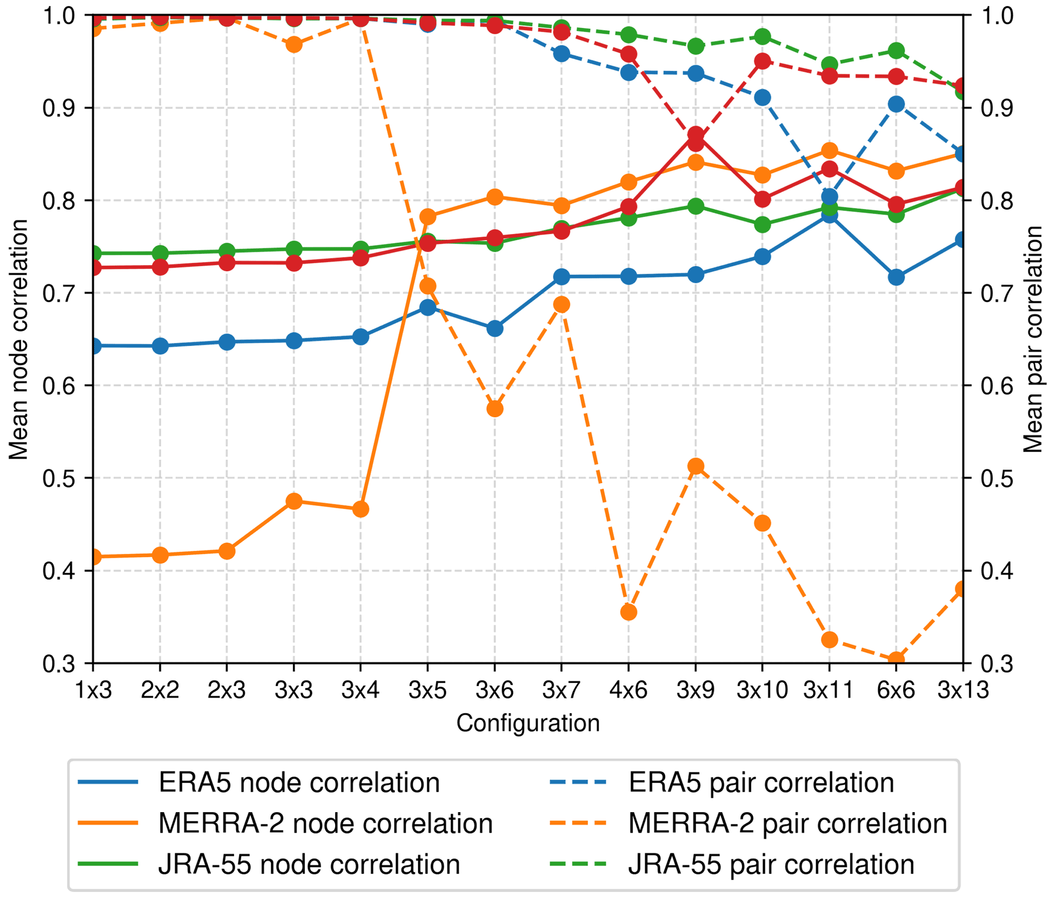
Figure B1Indicators of SOM realism and node uniqueness for different configurations (grid sizes). Solid lines are the mean node correlation and dashed lines the mean pair correlation for Casey (green), DDU (red), Mawson (blue) and Neumayer (orange).
SOMs for Casey, Mawson and DDU were found to be relatively insensitive to the number of nodes, with very little change in the above statistics until around a 3×6 configuration (Fig. B1). Neumayer, on the other hand, is much more sensitive to the number of SOM nodes. This is likely because it is situated within a region of high MSLP variability (near the northern edge of the peak 12-hourly wind speed standard deviation in Fig. 1) compared to other stations where the local flow is much more constrained by orography. It could be argued then that a 3×5 configuration would be preferable for Neumayer. However, the performance of the reanalyses was found not to vary by node at Neumayer even for SOM grids with many nodes. For ease of interpretation, therefore, we opt for a grid with fewer nodes. Inclusion of additional SOM nodes at other stations was not found to add much value to the analysis except in distinguishing different varieties of extreme wind events, which is beyond the scope of the current work but may be useful for a more targeted analysis in future.
The effect of the length of the time series upon the selection of SOM configuration was also tested. Repeating the analysis used to produce Fig. B1 yielded very similar results with the time series artificially reduced from 8 years to 1. MSLP composites were also found to be very visually similar to Fig. 5, including when driven with hourly data instead of 12-hourly (not shown).
Overall, A SOM configuration of 2×3 was deemed to be capable of capturing critical differences in reanalysis performance (associated with katabatic and synoptic states as well as variations in flow orientation) without being too large for the reader to interpret easily.
The katabatic index used in this paper is calculated as
where g is acceleration due to gravity and α is the angle of the slope in the direction for which K is evaluated. The terms θ0 and Δθ are, respectively, the “background” potential temperature if long-wave cooling of the surface layer was neglected, and the departure from this background. These terms therefore represent the perturbation to the lapse rate near the surface assumed to drive katabatic flow. Here, the value of θ0 is approximated by assuming a linear background lapse rate between 600 hPa and the surface, and extrapolating based on the potential temperature gradient between 500 and 600 hPa down to the ERA5 surface height. Δθ is then calculated by subtracting the observed surface potential temperature (linearly extrapolated from the pressure level closest to the surface to the ERA5 surface height) from θ0.
As shown in the paper for Casey station (Sect. 3.2.2), a visual comparison of scatterplots between SOM nodes is arguably more informative than summary statistics given the regime behaviour in the winds. To supplement this analysis, however, we here provide a ranking of reanalyses based upon four performance metrics calculated from station near-surface wind measurements, the correlation coefficient (r), root mean square error (RMSE), mean bias (MB), and bias in the interquartile range (IQRB).
We rank the performance of each reanalysis for each station by calculating each statistic separately for each SOM node (Table D1). Each reanalysis is assigned a ranking for that node and metric (1 for the best, 3 for the worst), which is then weighted by the frequency of that node. Summing the rankings for each metric gives a final score for that station. By this measure, the overall rankings for each station are as follows:
-
Casey: 1. ERA5, 2. JRA-55, 3. MERRA-2
-
DDU: 1. ERA5, 2. JRA-55, 3. MERRA-2
-
Mawson: 1. JRA-55, 2. MERRA-2, 3. ERA5
-
Neumayer: 1. ERA5, 2. MERRA-2, 3. JRA-55
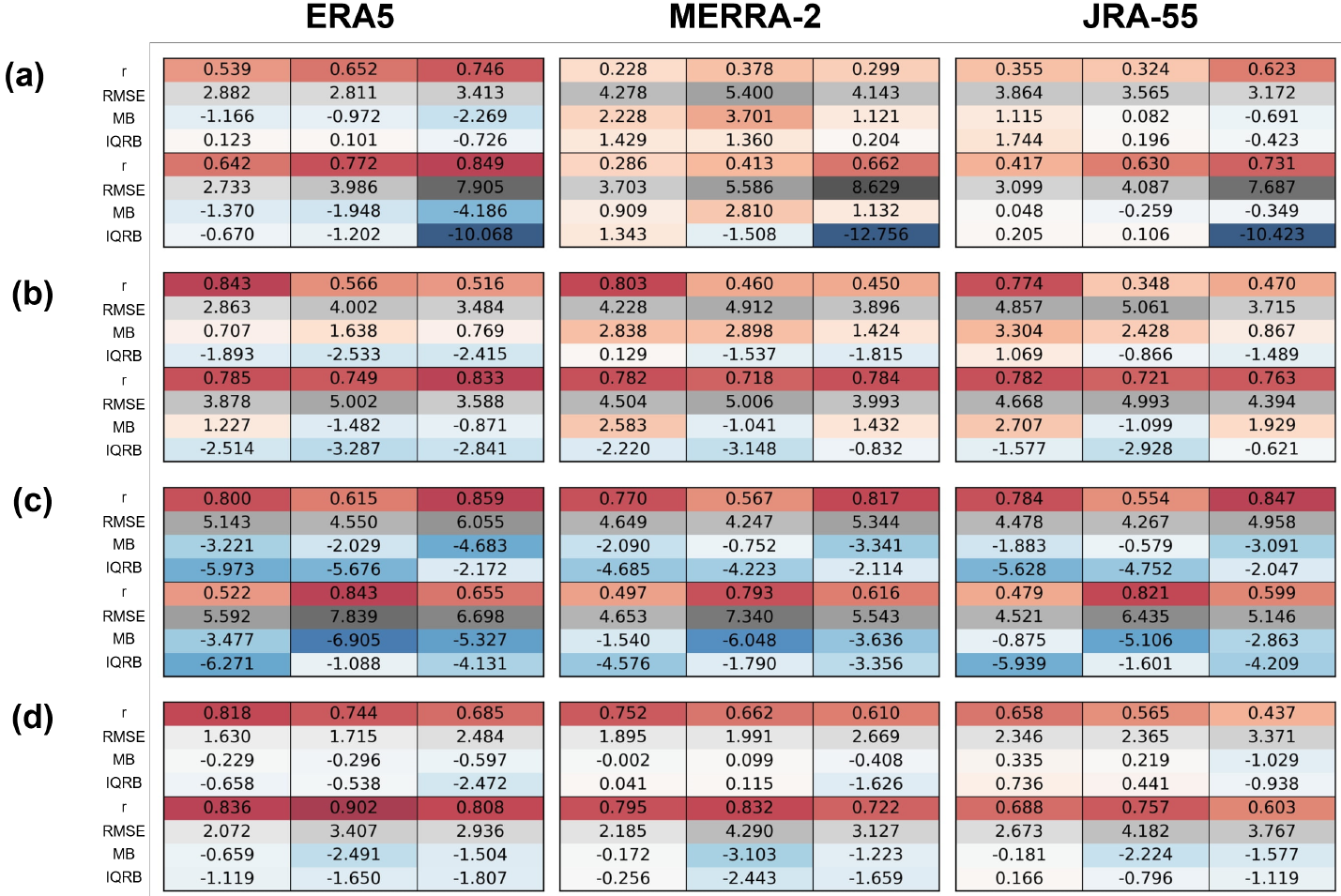
Table D1Performance statistics calculated from reanalysis vs. observed 12-hourly 10 m wind speed for (a) Casey, (b) DDU, (c) Mawson and (d) Neumayer. Left three columns correspond to ERA5, middle three MERRA-2 and right three JRA-55, with individual outlined boxes corresponding to SOM nodes as laid out in Fig. 5. Statistics shown include (by row) Pearson's correlation coefficient (r), root mean square error (RMSE, m s−1), mean bias (MB, m s−1), and reanalysis minus observed interquartile range (IQRB, m s−1).
Note that this ranking assigns equal weighting to each metric. If instead we sum across stations and rank by metric the results are as follows:
-
r: 1. ERA5, 2. MERRA-2, 3. JRA-55
-
RMSE: 1. ERA5, 2. JRA-55, 3. MERRA-2
-
MB: 1. JRA-55, 2. MERRA-2, 3. ERA5
-
IQRB: 1. JRA-55, 2. MERRA-2, 3. ERA5
ERA5 reanalysis data can be accessed from the Climate Data Store at https://cds.climate.copernicus.eu/cdsapp#!/home (last access: 10 November 2021; https://doi.org/10.24381/cds.adbb2d47, Hersbach et al., 2018b and https://doi.org/10.24381/cds.bd0915c6, Hersbach et al., 2018a). MERRA-2 can be accessed for surface-level data at https://doi.org/10.5067/3Z173KIE2TPD (GMAO, 2015a) and for pressure-level data at https://doi.org/10.5067/QBZ6MG944HW0 (GMAO, 2015b). JRA-55 can be accessed from the Research Data Archive at https://doi.org/10.5065/D6HH6H41 (Japan Meteorological Agency, 2013). C-2015 ASCAT data are produced by Remote Sensing Systems and sponsored by the NASA Ocean Vector Winds Science Team. Data are available at https://www.remss.com/missions/ascat/ (last access: 11 August 2021; Ricciardulli and Wentz, 2016). Radiosonde data from Neumayer station are available online at https://doi.org/10.1594/PANGAEA.874564 (König-Langlo, 2017). Other radiosonde datasets should be requested directly from the institutes referenced in the Acknowledgements. SCAR READER data are available online at https://www.bas.ac.uk/project/reader/ (last access: 5 April 2021; Colwell, 2002).
The supplement related to this article is available online at: https://doi.org/10.5194/wcd-3-1415-2022-supplement.
TCH led the analysis, interpretation of results and paper preparation with contributions from all co-authors. TCH and SB designed and implemented the analysis techniques and developed the analysis code. ÉV maintains and provided access to the high-resolution radiosonde data.
The contact author has declared that none of the authors has any competing interests.
Publisher’s note: Copernicus Publications remains neutral with regard to jurisdictional claims in published maps and institutional affiliations.
Thomas Caton Harrison and Stavroula Biri were funded by NERC grant “Improved projections of winds at the crossroads between Antarctica and the Southern Ocean” (NE/V000691/1 at BAS and NE/V000969/1 at NOC). This work forms part of the Polar Science for Planet Earth program of the British Antarctic Survey. We are grateful to the European Centre for Medium-range Weather Forecasts (ECMWF), the NASA Global Modeling and Assimilation Office (GMAO) and the Japan Meteorological Agency (JMA) for making ERA5, MERRA-2 and JRA-55 available, respectively. For radiosonde data from Casey and Mawson station, we thank the Australian Bureau of Meteorology. For radiosonde data from Neumauyer, we gratefully acknowledge König-Langlo (2017) who make the data openly available at the link in the data statement. For radiosonde data from Dumont d'Urville, we thank Météo France, the DSO/DOA service for the acquisition and distribution of the data. We are grateful to Steve Colwell for supporting and disseminating the READER dataset. C-2015 ASCAT data are produced by remote sensing systems and sponsored by the NASA Ocean Vector Winds Science Team. Data are available at http://www.remss.com (last access: 11 August 2021); thanks to ICDC, CEN, University of Hamburg for data support. We also thank two anonymous reviewers whose insightful comments helped to improve the paper.
This research has been supported by the Natural Environment Research Council (NERC; Improved projections of winds at the crossroads between Antarctica and the Southern Ocean (grant nos. NE/V000691/1 and NE/V000969/1)).
This paper was edited by Tiina Nygård and reviewed by two anonymous referees.
Adams, N.: A numerical modeling study of the weather in East Antarctica and the surrounding Southern Ocean, Weather Forecast., 19, 653–672, 2004. a
Ball, F. K.: Winds on the ice slopes of Antarctica, in: Antarctic Meteorology: Proceedings of the Symposium Held in Melbourne, February 1959, Australian Academy of Science, 9–16, 1960. a
Belmonte Rivas, M. and Stoffelen, A.: Characterizing ERA-Interim and ERA5 surface wind biases using ASCAT, Ocean Sci., 15, 831–852, https://doi.org/10.5194/os-15-831-2019, 2019. a, b, c
Boullot, N., Rabier, F., Langland, R., Gelaro, R., Cardinali, C., Guidard, V., Bauer, P., and Doerenbecher, A.: Observation impact over the southern polar area during the Concordiasi field campaign, Q. J. Roy. Meteorol. Soc., 142, 597–610, 2016. a
Bourassa, M. A., Meissner, T., Cerovecki, I., Chang, P. S., Dong, X., De Chiara, G., Donlon, C., Dukhovskoy, D. S., Elya, J., Fore, A., Fewings, M. R., Foster, R. C., Gille, S. T., Haus, B. K., Hristova-Veleva, S., Holbach, H. M., Jelenak, Z., Knaff, J. A., Kranz, S. A., Manaster, A., Mazloff, M., Mears, C., Mouche, A., Portabella, M., Reul, N., Ricciardulli, L., Rodriguez, E., Sampson, C., Solis, D., Stoffelen, A., Stukel, M. R., Stiles, B., Weissman, D., and Wentz, F.: Remotely sensed winds and wind stresses for marine forecasting and ocean modeling, Frontiers in Marine Science, 6, 443, https://doi.org/10.3389/fmars.2019.00443, 2019. a
Bromwich, D. H., Powers, J. G., Manning, K. W., and Zou, X.: Antarctic Data Impact Experiments with Polar WRF During the YOPP-SH Summer Special Observing Period, Q. J. Roy. Meteor. Soc., 2022. a
Carvalho, D.: An assessment of NASA’s GMAO MERRA-2 reanalysis surface winds, J. Climate, 32, 8261–8281, 2019. a, b
Cassano, E. N., Glisan, J. M., Cassano, J. J., Gutowski Jr., W. J., and Seefeldt, M. W.: Self-organizing map analysis of widespread temperature extremes in Alaska and Canada, Clim. Res., 62, 199–218, 2015. a
Colwell, S: Long-term dataset of mean surface and upper air meteorological measurements from a selection of Antarctic stations and automatic weather stations - READER (REference Antarctic Data for Environmental Research) project, British Antarctic Survey (BAS) [data set], https://www.bas.ac.uk/project/reader/ (last access: 5 April 2021), 2002. a
De Chiara, G., Bonavita, M., and English, S. J.: Improving the assimilation of scatterometer wind observations in global NWP, IEEE J. Sel. Top. Appl., 10, 2415–2423, 2017. a
de Kloe, J., Stoffelen, A., and Verhoef, A.: Improved use of scatterometer measurements by using stress-equivalent reference winds, IEEE J. Sel. Top. Appl., 10, 2340–2347, 2017. a
Dong, X., Wang, Y., Hou, S., Ding, M., Yin, B., and Zhang, Y.: Robustness of the recent global atmospheric reanalyses for Antarctic near-surface wind speed climatology, J. Climate, 33, 4027–4043, 2020. a, b, c
Francis, D., Mattingly, K. S., Lhermitte, S., Temimi, M., and Heil, P.: Atmospheric extremes caused high oceanward sea surface slope triggering the biggest calving event in more than 50 years at the Amery Ice Shelf, The Cryosphere, 15, 2147–2165, https://doi.org/10.5194/tc-15-2147-2021, 2021. a
Fulton, S. R., Schubert, W. H., Chen, Z., and Ciesielski, P. E.: A Dynamical Explanation of the Topographically Bound Easterly Low-Level Jet Surrounding Antarctica, J. Geophys. Res.-Atmos., 122, 12–635, 2017. a, b
Ganeshan, M. and Yang, Y.: Evaluation of the Antarctic boundary layer thermodynamic structure in MERRA2 using dropsonde observations from the Concordiasi campaign, Earth and Space Science, 6, 2397–2409, 2019. a
Gelaro, R., McCarty, W., Suárez, M. J., Todling, R., Molod, A., Takacs, L., Randles, C. A., Darmenov, A., Bosilovich, M. G., Reichle, R., Wargan, K., Coy, L., Cullather, R., Draper, C., Akella, S., Buchard, V., Conaty, A., da Silva, A. M., Gu, W., Kim, G., Koster, R., Lucchesi, R., Merkova, D., Nielsen, J. E., Partyka, G., Pawson, S., Putman, W., Rienecker, M., Schubert, S. D., Sienkiewicz, M., and Zhao, B.: The modern-era retrospective analysis for research and applications, Version 2 (MERRA-2), J. Climate, 30, 5419–5454, 2017. a, b
Gibson, P. B., Perkins-Kirkpatrick, S. E., Uotila, P., Pepler, A. S., and Alexander, L. V.: On the use of self-organizing maps for studying climate extremes, J. Geophys. Res.-Atmos., 122, 3891–3903, 2017. a, b
GMAO (Global Modeling and Assimilation Office): MERRA-2 inst1_2d_asm_Nx: 2d,1-Hourly,Instantaneous,Single-Level,Assimilation,Single-Level Diagnostics V5.12.4, Goddard Earth Sciences Data and Information Services Center (GES DISC) [data set], Greenbelt, MD, USA, https://doi.org/10.5067/3Z173KIE2TPD, 2015a. a
GMAO (Global Modeling and Assimilation Office): MERRA-2 inst3_3d_asm_Np: 3d,3-Hourly,Instantaneous,Pressure-Level,Assimilation,Assimilated Meteorological Fields V5.12.4, Goddard Earth Sciences Data and Information Services Center (GES DISC) [data set], Greenbelt, MD, USA, https://doi.org/10.5067/QBZ6MG944HW0, 2015b. a
GMAO (Global Modeling and Assimilation Office): MERRA-2 tavg1_2d_flx_Nx: 2d, 1-Hourly, Time-Averaged, Single-Level, Assimilation, Surface Flux Diagnostics V5.12.4, Goddard Earth Sciences Data and Information Services Center (GES DISC) [data set], Greenbelt, MD, USA, https://doi.org/10.5067/7MCPBJ41Y0K6, 2015c. a
Goddard, P. B., Dufour, C. O., Yin, J., Griffies, S. M., and Winton, M.: CO2-induced ocean warming of the Antarctic continental shelf in an eddying global climate model, J. Geophys. Res.-Oceans, 122, 8079–8101, 2017. a
Gorodetskaya, I. V., Silva, T., Schmithüsen, H., and Hirasawa, N.: Atmospheric river signatures in radiosonde profiles and reanalyses at the Dronning Maud Land coast, East Antarctica, Adv. Atmos. Sci., 37, 455–476, 2020. a
Gossart, A., Helsen, S., Lenaerts, J., Broucke, S. V., Van Lipzig, N., and Souverijns, N.: An evaluation of surface climatology in state-of-the-art reanalyses over the Antarctic Ice Sheet, J. Climate, 32, 6899–6915, 2019. a, b
Hazel, J. E. and Stewart, A. L.: Are the near-Antarctic easterly winds weakening in response to enhancement of the southern annular mode?, J. Climate, 32, 1895–1918, 2019. a
Hazel, J. E. and Stewart, A. L.: Bistability of the Filchner-Ronne Ice Shelf Cavity Circulation and Basal Melt, J. Geophys. Res.-Oceans, 125, e2019JC015848, https://doi.org/10.1029/2019JC015848, 2020. a
Hersbach, H.: Assimilation of scatterometer data as equivalent-neutral wind, ECMWF, 2010. a
Hersbach, H., Bell, B., Berrisford, P., Biavati, G., Horányi, A., Muñoz Sabater, J., Nicolas, J., Peubey, C., Radu, R., Rozum, I., Schepers, D., Simmons, A., Soci, C., Dee, D., and Thépaut, J.-N.: ERA5 hourly data on pressure levels from 1959 to present, Copernicus Climate Change Service (C3S) Climate Data Store (CDS) [data set], https://doi.org/10.24381/cds.bd0915c6, 2018a (data available at: https://cds.climate.copernicus.eu/cdsapp#!/home, last access: 10 November 2021). a
Hersbach, H., Bell, B., Berrisford, P., Biavati, G., Horányi, A., Muñoz Sabater, J., Nicolas, J., Peubey, C., Radu, R., Rozum, I., Schepers, D., Simmons, A., Soci, C., Dee, D., and Thépaut, J.-N.: ERA5 hourly data on single levels from 1959 to present, Copernicus Climate Change Service (C3S) Climate Data Store (CDS) [data set], https://doi.org/10.24381/cds.adbb2d47, 2018b (data available at: https://cds.climate.copernicus.eu/cdsapp#!/home, last access: 10 November 2021). a
Hersbach, H., Bell, B., Berrisford, P., et al.: The ERA5 global reanalysis, Q. J. Roy. Meteor. Soc., 146, 1999–2049, 2020. a, b, c
Hewitson, B. C. and Crane, R. G.: Self-organizing maps: applications to synoptic climatology, Clim. Res., 22, 13–26, 2002. a
Japan Meteorological Agency: JRA-55: Japanese 55-year Reanalysis, Daily 3-Hourly and 6-Hourly Data, Research Data Archive at the National Center for Atmospheric Research, Computational and Information Systems Laboratory [data set], Boulder, CO, https://doi.org/10.5065/D6HH6H41, 2013. a
Jena, B., Bajish, C., Turner, J., Ravichandran, M., Anilkumar, N., and Kshitija, S.: Record low sea ice extent in the Weddell Sea, Antarctica in April/May 2019 driven by intense and explosive polar cyclones, npj Climate and Atmospheric Science, 5, 1–15, 2022. a
Jolly, B., Mcdonald, A. J., Coggins, J. H., Zawar-Reza, P., Cassano, J., Lazzara, M., Graham, G., Plank, G., Petterson, O., and Dale, E.: A validation of the Antarctic mesoscale prediction system using self-organizing maps and high-density observations from SNOWWEB, Mon. Weather Rev., 144, 3181–3200, 2016. a
Jones, R., Renfrew, I., Orr, A., Webber, B., Holland, D., and Lazzara, M.: Evaluation of four global reanalysis products using in situ observations in the Amundsen Sea Embayment, Antarctica, J. Geophys. Res.-Atmos., 121, 6240–6257, 2016. a, b, c
King, J., Connolley, W., and Derbyshire, S.: Sensitivity of modelled Antarctic climate to surface and boundary-layer flux parametrizations, Q. J. Roy. Meteor. Soc., 127, 779–794, 2001. a
Klöwer, M., Jung, T., König-Langlo, G., and Semmler, T.: Aspects of weather parameters at Neumayer station, Antarctica, and their representation in reanalysis and climate model data, Meteorol. Z., https://doi.org/10.1127/0941-2948/2013/0505, 2014. a
Kobayashi, S., Ota, Y., Harada, Y., Ebita, A., Moriya, M., Onoda, H., Onogi, K., Kamahori, H., Kobayashi, C., Endo, H., Miyaoka, K., and Takahashi, K.: The JRA-55 reanalysis: General specifications and basic characteristics, J. Meteorol. Soc. Jpn. Ser. II, 93, 5–48, 2015. a, b, c
König-Langlo, G.: Radiosonde measurements from Neumayer Station (2016-12), Alfred Wegener Institute, Helmholtz Centre for Polar and Marine Research, Bremerhaven, PANGAEA [data set], https://doi.org/10.1594/PANGAEA.874564, 2017. a, b
König-Langlo, G., King, J., and Pettré, P.: Climatology of the three coastal Antarctic stations Dumont d'Urville, Neumayer, and Halley, J. Geophys. Res.-Atmos., 103, 10935–10946, 1998. a
Koster, R. D., McCarty, W., Coy, L., Gelaro, R., Huang, A., Merkova, D., Smith, E. B., Sienkiewicz, M. and Wargan, K.. MERRA-2 input observations: Summary and assessment, No. GSFC-E-DAA-TN37524, 2016. a
Kottmeier, C.: The influence of baroclinicity and stability on the wind and temperature conditions at the Georg von Neumayer Antarctic station, Tellus A, 38, 263–276, 1986. a
Kurtz, D. D. and Bromwich, D. H.: A recurring, atmospherically forced polynya in Terra Nova Bay, Oceanology of the Antarctic Continental Shelf, 43, 177–201, 1985. a
Liu, H., Jezek, K. C., Li, B., and Zhao, Z.: Radarsat Antarctic Mapping Project Digital Elevation Model, Version 2, NASA National Snow and Ice Data Center Distributed Active Archive Center [data set], Boulder, Colorado USA, https://doi.org/10.5067/8JKNEW6BFRVD, 2015. a
Mathiot, P., Jourdain, N. C., Barnier, B., Gallée, H., Molines, J. M., Le Sommer, J., and Penduff, T.: Sensitivity of coastal polynyas and high-salinity shelf water production in the Ross Sea, Antarctica, to the atmospheric forcing, Ocean Dynam., 62, 701–723, 2012. a
Moore, G., Bromwich, D. H., Wilson, A. B., Renfrew, I., and Bai, L.: Arctic System Reanalysis improvements in topographically forced winds near Greenland, Q. J. Roy. Meteor. Soc., 142, 2033–2045, 2016. a
Murphy, B. F. and Simmonds, I.: An analysis of strong wind events simulated in a GCM near Casey in the Antarctic, Mon. Weather Rev., 121, 522–534, 1993. a
Nigro, M. A. and Cassano, J. J.: Analysis of the Ross Ice Shelf airstream forcing mechanisms using self-organizing maps, Mon. Weather Rev., 142, 4719–4734, 2014a. a
Nigro, M. A. and Cassano, J. J.: Identification of surface wind patterns over the Ross Ice Shelf, Antarctica, using self-organizing maps, Mon. Weather Rev., 142, 2361–2378, 2014b. a
Orr, A., Phillips, T., Webster, S., Elvidge, A., Weeks, M., Hosking, S., and Turner, J.: Met Office Unified Model high-resolution simulations of a strong wind event in Antarctica, Q. J. Roy. Meteor. Soc., 140, 2287–2297, 2014. a, b, c, d
Parish, T. R. and Bromwich, D. H.: The surface windfield over the Antarctic ice sheets, Nature, 328, 51–54, 1987. a
Parish, T. R. and Cassano, J. J.: Forcing of the wintertime Antarctic boundary layer winds from the NCEP–NCAR global reanalysis, J. Appl. Meteorol., 40, 810–821, 2001. a
Parish, T. R. and Cassano, J. J.: The role of katabatic winds on the Antarctic surface wind regime, Mon. Weather Rev., 131, 317–333, 2003. a, b
Petrelli, P., Bindoff, N., and Bergamasco, A.: The sea ice dynamics of Terra Nova Bay and Ross Ice Shelf Polynyas during a spring and winter simulation, J. Geophys. Res.-Oceans, 113, C09003, https://doi.org/10.1029/2006JC004048, 2008. a
Renfrew, I. A., Barrell, C., Elvidge, A., Brooke, J., Duscha, C., King, J., Kristiansen, J., Cope, T. L., Moore, G. W. K., Pickart, R. S., Reuder, J., Sandu, I., Sergeev, D., Terpstra, A., Våge, K., and Weiss, A.: An evaluation of surface meteorology and fluxes over the Iceland and Greenland Seas in ERA5 reanalysis: The impact of sea ice distribution, Q. J. Roy. Meteor. Soc., 147, 691–712, 2021. a
Ricciardulli, L. and Wentz, F. J.: Remote Sensing Systems ASCAT C-2015 Daily Ocean Vector Winds on 0.25 deg grid, Version 02.1, Remote Sensing Systems [data set], Santa Rosa, CA, https://www.remss.com/missions/ascat/ (last access: 11 August 2021), 2016. a, b, c
Sampe, T. and Xie, S.-P.: Mapping high sea winds from space: A global climatology, B. Am. Meteorol. Soc., 88, 1965–1978, 2007. a
Schmidt, K. M., Swart, S., Reason, C., and Nicholson, S.-A.: Evaluation of satellite and reanalysis wind products with in situ wave glider wind observations in the Southern Ocean, J. Atmos. Ocean. Tech., 34, 2551–2568, 2017. a
Scott, R. C., Nicolas, J. P., Bromwich, D. H., Norris, J. R., and Lubin, D.: Meteorological drivers and large-scale climate forcing of West Antarctic surface melt, J. Climate, 32, 665–684, 2019. a
Silvano, A., Foppert, A., Rintoul, S. R., Holland, P. R., Tamura, T., Kimura, N., Castagno, P., Falco, P., Budillon, G., Haumann, F. A., Naveira Garabato, A. C., and Macdonald, A. M.: Recent recovery of Antarctic Bottom Water formation in the Ross Sea driven by climate anomalies, Nat. Geosci., 13, 780–786, 2020. a
Skific, N. and Francis, J.: Self-organizing maps: a powerful tool for the atmospheric sciences, Applications of self-organizing maps, 251–268, https://doi.org/10.5772/54299, 2012. a
Spence, P., Griffies, S. M., England, M. H., Hogg, A. M., Saenko, O. A., and Jourdain, N. C.: Rapid subsurface warming and circulation changes of Antarctic coastal waters by poleward shifting winds, Geophys. Res. Lett., 41, 4601–4610, 2014. a
Stewart, A. L. and Thompson, A. F.: Sensitivity of the ocean's deep overturning circulation to easterly Antarctic winds, Geophys. Res. Lett., 39, L18604, https://doi.org/10.1029/2012GL053099, 2012. a
Stewart, A. L., Klocker, A., and Menemenlis, D.: Acceleration and overturning of the Antarctic Slope Current by winds, eddies, and tides, J. Phys. Oceanogr., 49, 2043–2074, 2019. a
Tetzner, D., Thomas, E., and Allen, C.: A validation of ERA5 reanalysis data in the Southern Antarctic Peninsula–Ellsworth land region, and its implications for ice core studies, Geosciences, 9, 289, https://doi.org/10.3390/geosciences9070289, 2019. a, b
Thompson, A. F., Stewart, A. L., Spence, P., and Heywood, K. J.: The Antarctic Slope Current in a changing climate, Rev. Geophys., 56, 741–770, 2018. a
Tomikawa, Y., Nomoto, M., Miura, H., Tsutsumi, M., Nishimura, K., Nakamura, T., Yamagishi, H., Yamanouchi, T., Sato, T., and Sato, K.: Vertical wind disturbances during a strong wind event observed by the PANSY radar at Syowa Station, Antarctica, Mon. Weather Rev., 143, 1804–1821, 2015. a
Torralba, V., Doblas-Reyes, F. J., and Gonzalez-Reviriego, N.: Uncertainty in recent near-surface wind speed trends: a global reanalysis intercomparison, Environ. Res. Lett., 12, 114019, https://doi.org/10.1088/1748-9326/aa8a58, 2017. a, b
Truong, S., Huang, Y., Lang, F., Messmer, M., Simmonds, I., Siems, S., and Manton, M.: A climatology of the marine atmospheric boundary layer over the Southern Ocean from four field campaigns during 2016–2018, J. Geophys. Res.-Atmos., 125, e2020JD033214, https://doi.org/10.1029/2020JD033214, 2020. a
Turner, J., Lachlan-Cope, T. A., Marshall, G. J., Pendlebury, S., and Adams, N.: An extreme wind event at Casey Station, Antarctica, J. Geophys. Res.-Atmos., 106, 7291–7311, 2001. a
Turner, J., Colwell, S. R., Marshall, G. J., Lachlan-Cope, T. A., Carleton, A. M., Jones, P. D., Lagun, V., Reid, P. A., and Iagovkina, S.: The SCAR READER project: toward a high-quality database of mean Antarctic meteorological observations, J. Climate, 17, 2890–2898, 2004. a
Turner, J., Chenoli, S. N., Abu Samah, A., Marshall, G., Phillips, T., and Orr, A.: Strong wind events in the Antarctic, J. Geophys. Res.-Atmos., 114, D18103, https://doi.org/10.1029/2008JD011642, 2009. a
van den Broeke, M. and van Lipzig, N.: Factors controlling the near-surface wind field in Antarctica, Mon. Weather Rev., 131, 733–743, 2003. a, b, c, d, e
Vignon, É., Traullé, O., and Berne, A.: On the fine vertical structure of the low troposphere over the coastal margins of East Antarctica, Atmos. Chem. Phys., 19, 4659–4683, https://doi.org/10.5194/acp-19-4659-2019, 2019. a, b, c, d, e, f, g, h, i
Vignon, É., Picard, G., Durán-Alarcón, C., Alexander, S. P., Gallée, H., and Berne, A.: Gravity wave excitation during the coastal transition of an extreme katabatic flow in Antarctica, J. Atmos. Sci., 77, 1295–1312, 2020. a
Wang, X., Zhang, Z., Wang, X., Vihma, T., Zhou, M., Yu, L., Uotila, P., and Sein, D. V.: Impacts of strong wind events on sea ice and water mass properties in Antarctic coastal polynyas, Clim. Dynam., 57, 3505–3528, 2021. a
Weber, N. J., Lazzara, M. A., Keller, L. M., and Cassano, J. J.: The extreme wind events in the ross island region of Antarctica, Weather Forecast., 31, 985–1000, 2016. a
Wittek, P., Gao, S. C., Lim, I. S., and Zhao, L.: somoclu: An Efficient Parallel Library for Self-Organizing Maps, J. Stat. Softw., 78, 1–21, https://doi.org/10.18637/jss.v078.i09, 2017. a
Yamada, K. and Hirasawa, N.: Analysis of a Record-Breaking Strong Wind Event at Syowa Station in January 2015, J. Geophys. Res.-Atmos., 123, 13–643, 2018. a
Yu, Y. and Cai, X.-M.: Structure and dynamics of katabatic flow jumps: Idealised simulations, Bound.-Lay. Meteorol., 118, 527–555, 2006. a
- Abstract
- Introduction
- Data and methods
- Results
- Discussion
- Conclusions
- Appendix A: Collocation sensitivity test
- Appendix B: Selection of SOM configuration
- Appendix C: Calculation of katabatic index
- Appendix D: Detailed SOM state statistics
- Data availability
- Author contributions
- Competing interests
- Disclaimer
- Acknowledgements
- Financial support
- Review statement
- References
- Supplement