the Creative Commons Attribution 4.0 License.
the Creative Commons Attribution 4.0 License.
 | 01 Dec 2023
Variations in boundary layer stability across Antarctica: a comparison between coastal and interior sites
Mckenzie J. Dice
John J. Cassano
Gina C. Jozef
Mark Seefeldt
The range of boundary layer stability profiles, from the surface to 500 m a.g.l. (above ground level), present in radiosonde observations from two continental-interior (South Pole Station and Dome Concordia Station) and three coastal (McMurdo Station, Georg von Neumayer Station III, and Syowa Station) Antarctic sites, is examined using the self-organizing maps (SOMs) neural network algorithm. A wide range of potential temperature profiles is revealed, from shallow boundary layers with strong near-surface stability to deeper boundary layers with weaker or near-neutral stability, as well as profiles with weaker near-surface stability and enhanced stability aloft, above the boundary layer. Boundary layer regimes were defined based on the range of profiles revealed by the SOM analysis; 20 boundary layer regimes were identified to account for differences in stability near the surface as well as above the boundary layer. Strong, very strong, or extremely strong stability, with vertical potential temperature gradients of 5 to in excess of 30 K per 100 m, occurred more than 80 % of the time at South Pole and Dome Concordia in the winter. Weaker stability was found in the winter at the coastal sites, with moderate and strong stability (vertical potential temperature gradients of 1.75 to 15 K per 100 m) occurring 70 % to 85 % of the time. Even in the summer, moderate and strong stability is found across all five sites, either immediately near the surface or aloft, just above the boundary layer. While the mean boundary layer height at the continental-interior sites was found to be approximately 50 m, the mean boundary layer height at the coastal sites was deeper, around 110 m. Further, a commonly described two-stability-regime system in the Arctic associated with clear or cloudy conditions was applied to the 20 boundary layer regimes identified in this study to understand if the two-regime behavior is also observed in the Antarctic. It was found that moderate and strong stability occur more often with clear- than cloudy-sky conditions, but weaker stability regimes occur almost equally for clear and cloudy conditions.
- Article
(10521 KB) - Full-text XML
-
Supplement
(1654 KB) - BibTeX
- EndNote


-
Self-organizing maps are used to examine the range of boundary layer stability profiles at two continental and three coastal Antarctic sites.
-
Near-neutral to weak near-surface stability usually occurs half or more than half of the time in all seasons at the coastal sites but is infrequent at continental-interior sites, except in the summer.
-
When considering maximum stability near the surface or just above the boundary layer, moderate or stronger stability occurs almost always at the interior sites and often more than half of the time at the coastal sites.
-
At two of the three coastal sites analyzed here, moderate and strong stability occur more often with clear- than cloudy-sky conditions at one of the coastal sites; near-neutral and weak stability regimes occur more often with cloudy conditions.
Strong temperature inversions in Antarctica are the result of predominantly high-albedo ice-covered surfaces and a low sun angle in the summer and polar night in the winter. All these factors contribute to prolonged surface radiative cooling, which often results in statically stable boundary layers (King and Turner, 1997; Andreas et al., 2000) with temperature inversions sometimes exceeding 20 K (Lettau and Schwerdtfeger, 1967; Phillpot and Zillman, 1970; Connolley, 1996). Increased solar radiation and warmer surface temperatures can result in near-neutral or weakly stable conditions during the summer. Similar stability conditions can also occur at other times of year as a result of increased wind speeds or increased downwelling longwave radiation due to cloud cover (Hudson and Brandt, 2005; Stone and Kahl, 1991). This study aims to investigate the range of boundary layer stability that exists throughout the year at two continental-interior sites and three coastal sites in Antarctica (Fig. 1).
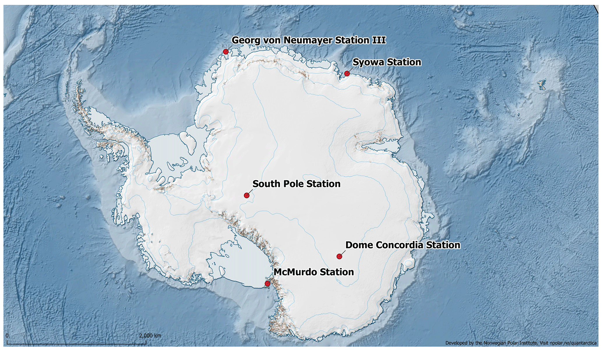
Figure 1Location of study sites (red dots with station names) across the Antarctic continent. Map courtesy of Quantarctica (Matsuoka et al., 2018).
A previous study for McMurdo Station analyzed the range of boundary layer stability regimes present during the year-long Department of Energy (DOE) Atmospheric Radiation Measurement (ARM) West Antarctic Radiation Experiment (AWARE) campaign (Dice and Cassano, 2022). A strong seasonality of varying boundary layer stability was found, with the winter conditions dominated by strongly stable boundary layers (61 % of the time) and summer conditions dominated by weak stability (83 % of the time). Increased wind speeds in the winter were found to be responsible for reducing strong near-surface stability. This reduction in stability occurred near the surface, while enhanced stability remained aloft in some cases. The results presented below aim to expand the analysis of boundary layer stability in Dice and Cassano (2022) to both continental and coastal locations across Antarctica.
Data from two additional coastal stations, Georg von Neumayer Station III (Neumayer Station) and Syowa Station (Fig. 1), will also be analyzed, in addition to revisiting the data at McMurdo Station described above. Previously published results found surface-based temperature inversions occurred year-round at Neumayer Station, with a maximum frequency in the winter and a minimum in the summer, with 75 % of the inversions having a strength of more than 1 K, as well as some up to 25 K, especially in the winter (König-Langlo and Loose, 2007; Silva et al., 2022). Some of the temperature profile structures observed by Silva et al. (2022) revealed multiple inversions within the same profile. This is similar to McMurdo Station, where enhanced stability was often found to exist above a layer of weaker stability (Dice and Cassano, 2022). Cassano et al. (2016) found that stable boundary layer conditions occur 83 % of the year over the northwestern Ross Ice Shelf (approximately 100 km from McMurdo Station), while neutral conditions occur 17 % of the time. Further, 50 % of the summer season was characterized by weakly unstable conditions, while stable stratification is dominant in the other three seasons (84 % to 94 %).
The continental interior of Antarctica is characterized by a short summer and a long, coreless winter (Hudson and Brandt, 2005). Stronger inversions and colder temperatures are often characteristic of higher-elevation continental-interior sites (Phillpot and Zillman, 1970; Comiso, 1994; Zhang et al., 2011), compared to coastal locations with weaker inversions and warmer temperatures (Phillpot and Zillman, 1970; Cassano et al., 2016). Continental-interior sites also have a greater inversion frequency than coastal sites, with the inversion frequency in the fall and winter close to 100 % (Zhang et al., 2011). At South Pole Station, inversions were found to be more common and stronger in the winter than in the summer. Hudson and Brandt (2005) also found inversions in the summer at Dome Concordia (Dome C) to be stronger than those at South Pole. Inversions near the surface at Dome C can reach to 1 K m−1 during polar night, and even stronger inversions, at 10 to 15 m above the surface, of up to 2.5 K m−1 have been observed (Genthon et al., 2013).
Boundary layer stability in the polar regions in the winter has often been described as existing in two distinct states (weak or strongly stable), driven by changes in cloud cover. The weakly stable regimes occur under cloudy conditions, with increased downwelling longwave radiation warming the surface and reducing stability. Cloudy conditions can also result in cloud-top radiative cooling and initiate convective mixing when the atmosphere is cooled aloft by the cloud (Chechin et al., 2023). In contrast, clear-sky conditions allow for strong radiative cooling and strong stability (Stone and Kahl, 1991; Mahrt, 1998, 2014; Solomon et al., 2023). Stone and Kahl (1991) described boundary layer stability at the South Pole as being in either a weakly stable or a strongly stable regime, associated with cloudy or clear conditions, respectively, throughout the summer of 1986. Solomon et al. (2023) distinguished between wintertime clear and cloudy regimes in the Arctic, during the Multidisciplinary Drifting Observatory for the Study of Arctic Climate (MOSAiC) campaign, to evaluate model predictions of near-surface meteorological conditions including boundary layer stability. They separated clear and cloudy regimes using the minima between the two peaks in the observed bimodal probability distribution function (PDF) of net longwave radiation. Following Solomon et al. (2023) we will identify clear and cloudy regimes based on the PDFs of net longwave radiation to determine if this bimodal view of clouds, as well as associated boundary layer stability, found in the Arctic is also applicable to coastal and interior sites across the Antarctic continent. We will also study how the clear–cloudy regimes relate to the continuous range of stability regimes identified in this study.
This paper begins with a description of the observations from five Antarctic sites and details of the methods used to analyze the data at these sites (Sect. 2). The results of this analysis will describe the range and frequency of boundary layer stability profiles (up to 500 m a.g.l.; above ground level) at the sites (Sect. 3). Additionally, differences in boundary layer stability associated with clear and cloudy conditions will be presented. The Results section will be followed by a discussion and comparison across coastal versus continental-interior locations (Sect. 4). A summary of these findings will follow, and the next steps in this research will be identified (Sect. 5).
2.1 Data
The analysis presented in this paper is based on radiosonde and surface longwave radiation observations from three coastal (McMurdo Station, Neumayer Station, and Syowa Station) and two continental-interior sites (South Pole Station and Dome Concordia Station) (Fig. 1, Table 1; hereafter these five stations are referred to as McMurdo, Neumayer, Syowa, South Pole, and Dome C). The period of data used in the analysis at these five sites ranges from 13 months (McMurdo) to 19 years (Syowa). The differing time period evaluated at each site is due to varying amounts of time when radiosonde and radiation data are both continuously available, as well as periods of time when data were readily accessible. At McMurdo, this time period was chosen to coincide with the availability of both radiosonde and radiation data from the AWARE campaign, which were previously analyzed by Dice and Cassano (2022). The Neumayer dataset is shorter than those at Syowa, Dome C, and South Pole, as Neumayer was not fully operational until 2009 and, from 2009 to 2018, only 5 s temporal resolution radiosonde data were available. These data did not have sufficient vertical resolution for this study; thus only data after 2018 with 1 s temporal resolution were used. Syowa, Dome C, and South Pole all have longer continuous radiosonde and radiation datasets that are easily accessible, lasting more than approximately 15 years.
Table 1Information for each of the five study sites: South Pole, Dome C, McMurdo, Neumayer, and Syowa. From left to right, the columns indicate the study site; coordinates and elevation above sea level (a.s.l.) of each site; site location type; type of radiosonde and accuracy of the temperature and wind measurements, respectively; time period of the radiosonde launches; and number of radiosonde launches in the dataset.
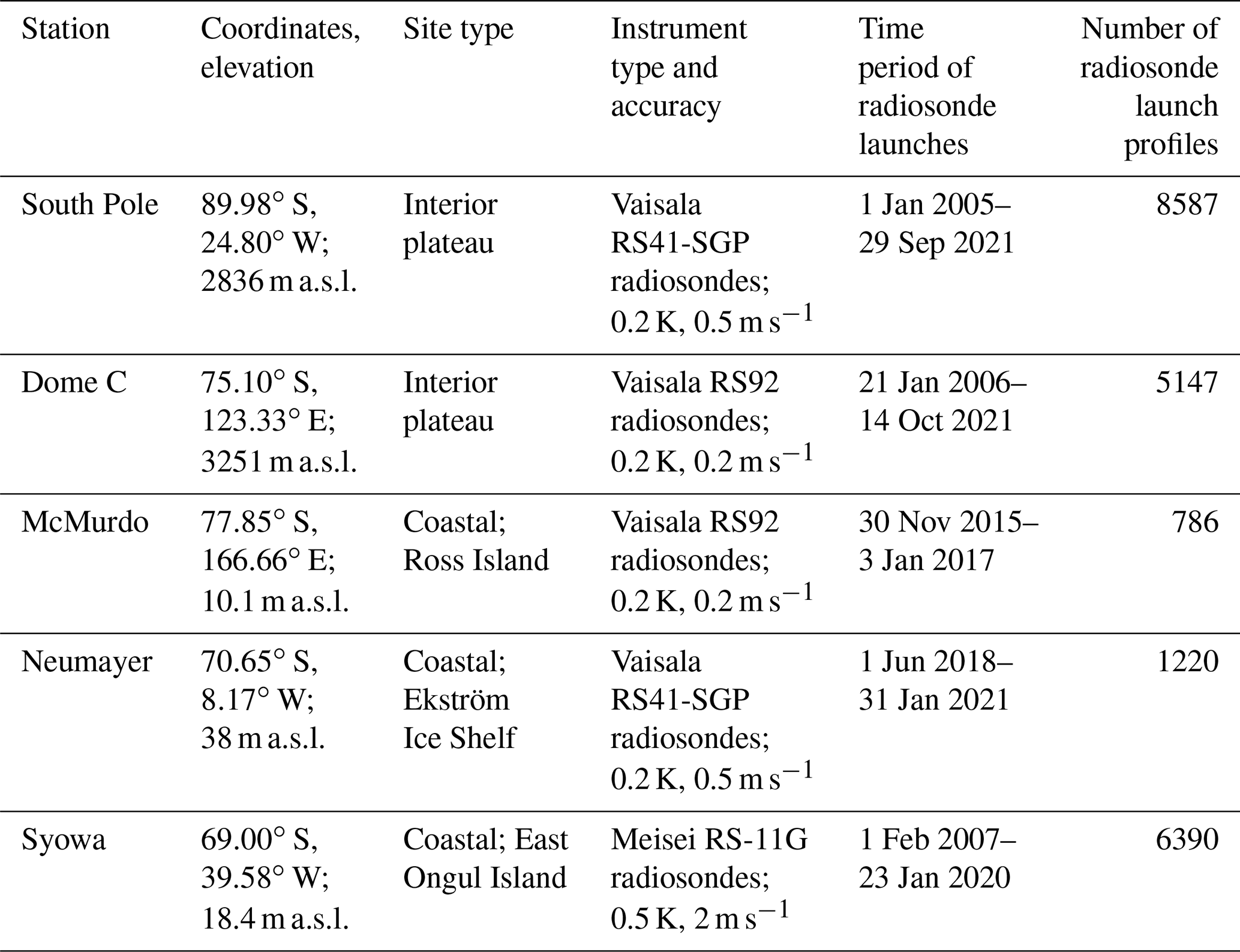
South Pole is a high-elevation (2835 m) continental-interior site where strong surface inversions and extremely cold temperatures dominate (Zhang et al., 2011) and strong stability is almost constantly observed, especially in the winter (Phillpot and Zillman, 1970). The radiosonde data from South Pole were retrieved from the Antarctic Meteorological Research and Data Center from 1 January 2005 to 29 September 2021. Radiosonde launches occur once daily at 21:00 UTC for most of the year, with twice-daily launches at approximately 09:00 and 21:00 UTC during the short austral summer. These launches occur at 22:00 and 10:00 LT (local time), respectively.
Dome C is another high-elevation (3233 m) continental-interior site characterized by cold temperatures and strong surface inversions, which occur throughout most of the year and in the winter on a nearly permanent basis (Genthon et al., 2013; Pietroni et al., 2013; Vignon et al., 2017). The radiosonde data from Dome C are provided by the Antarctic Meteo-Climatological Observatory from 21 January 2006 to 14 October 2021. The radiosonde launches at Dome C are performed once daily at 12:00 UTC year-round. It is important to note here that the 12:00 UTC soundings are at 04:00 LT, which is early morning at Dome C. Thus, at this time, the profiles from the radiosondes are likely to be reflective of shallower, more stable boundary layer conditions, rather than convective conditions, which are sometimes observed in near-surface observations during mid-day or in the summer at Dome C (Mastrantonio et al., 1999; Pietroni et al., 2013).
McMurdo is a coastal site located at the edge of the Ross Ice Shelf on the southwestern tip of Ross Island. The proximity of the Ross Ice Shelf, sea ice, open water, and the complex local topography near McMurdo result in a wide range of boundary layer stability types compared to the continental-interior sites (Dice and Cassano, 2022). The McMurdo radiosonde data are from the DOE AWARE campaign (Lubin et al., 2017, 2020; Silber et al., 2018), which occurred at McMurdo from 20 November 2015 to 3 January 2017. The radiosonde launches during AWARE occurred twice per day at 10:00 and 22:00 UTC (23:00 and 11:00 LT, respectively).
Neumayer is near sea level and located on the Ekström Ice Shelf, a relatively flat and homogeneous site. The meteorology and near-surface conditions are frequently influenced by large-scale cyclonic activity and sea ice fluctuations (Silva et al., 2022), resulting in changing boundary layer conditions. The radiosonde data from Neumayer are from the Baseline Surface Radiation Network (BSRN) from 1 June 2018 to 31 January 2021. Radiosonde launches occur once daily at approximately 12:00 UTC and twice daily during the summer months when conditions allow at 05:00 and 12:00 UTC (where UTC is local time).
Syowa is located on East Ongul Island in Lutzow-Holm Bay near sea level, with some low-elevation slopes around it, and like the other coastal sites, it experiences warmer surface temperatures compared to the continental interior. Syowa also experiences occasional strong wind due to katabatic flow from the continental interior (Murakoshi, 1958). The radiosonde data from Syowa are from the Office of Antarctic Observation Japan Meteorological Agency (Yutaka Ogawa, personal communication, 2021) from 1 February 2001 to 23 January 2020. Radiosonde launches occur twice daily at 11:30 and 23:30 UTC (14:30 and 02:30 LT, respectively).
Longwave radiation data were also obtained for all five sites to identify the clear- and cloudy-sky conditions following the methods from Solomon et al. (2023). The radiation data are from the BSRN, except at McMurdo, where the data are from the AWARE campaign.
2.2 Methods
2.2.1 Self-organizing map
The goal of this paper is to analyze and compare the variability in boundary layer stability, defined by potential temperature profiles, at five Antarctic research stations (Fig. 1). Hundreds to thousands of radiosonde profiles (Table 1), for each of the five sites, will be analyzed. The self-organizing map, or SOM, algorithm is used to objectively identify patterns in the potential temperature profiles that represent the range of conditions in the radiosonde observations.
The SOM algorithm is an unsupervised artificial neural network that groups similar patterns in the training data into a user-specified number of patterns, which span the range of conditions in the training data. The iterative training proceeds until the squared difference between the training data and the SOM patterns is minimized (Kohonen et al., 1996; Hewitson and Crane, 2002; Cassano et al., 2015). The resulting two-dimensional array of patterns is the master SOM, or simply the SOM. The SOM is organized such that similar patterns are located adjacent to each other, while the most distinct patterns are on opposite sides (Cassano et al., 2016). The SOMs presented here are trained using potential temperature gradient profiles from the radiosonde observations. The potential temperature gradient profiles () were used to train the SOM because this gradient defines the local static stability in the profile and allows for classification of boundary layer stability regimes across seasons and sites. The SOMs in this study were trained using the SOM-PAK software (http://www.cis.hut.fi/research/som-research, last access: October 2022), the details of which are described by Kohonen et al. (1996).
The radiosonde data are interpolated onto a regular vertical grid before applying the SOM algorithm, as described in Dice and Cassano (2022). Radiosonde profiles from all sites were interpolated to a 5 m grid from 20 to 500 m a.g.l. The lowest height of 20 m was selected since near-surface warm-biased temperatures are often present in radiosonde data observed below this height in many profiles at the five study sites (Schwartz and Doswell, 1991; Mahesh et al., 1997). The top height of 500 m was chosen since this height encompasses the boundary layer features of interest. It is also important to note here that the boundary layer in Antarctica has been observed to be shallower, with stable conditions extending further to the surface, than the 20 m bottom height in the profiles used in this analysis (e.g., Handorf et al., 1999). However, below this height in the radiosonde profiles, anomalously warm-biased temperatures are important to exclude, since this will indicate weaker stability than is actually present during the radiosonde launches.
To decide on the number of patterns to be identified by the SOM algorithm, several tests were performed to find the appropriate SOM size to adequately represent the range of boundary layer profiles present at each of the five sites. Unlike other iterative, unsupervised training algorithms, the SOM does not identify distinct patterns but rather a range of patterns which vary smoothly across the boundary layer states observed in the radiosonde data. Identifying the proper SOM size is important for visualizing the full range of boundary layer stability profiles present in the training data (Reusch et al., 2005; Cassano et al., 2015). Too small of a SOM will result in important differences in the training data being lost in the few generalized patterns, and too large of a SOM will be difficult to visualize, and only a few samples from the training data may correspond, or “map”, to each SOM pattern. Several SOM sizes were tested for this analysis: 3×2 (6 patterns), 4×3 (12 patterns), 5×4 (20 patterns), 6×5 (30 patterns), and 7×6 (42 patterns). This initial evaluation of different SOM sizes found that a 6×5 SOM (Figs. 2, 4, 6, 8, and 10) best represented the boundary layer states present across the training data at all five sites. The 30 patterns in the 6×5 SOM span the range of potential temperature profile types present in the training data, representing the hundreds to thousands of profiles (Table 1) from each of the five sites.
Once the SOM is trained, each individual radiosonde profile from the training data is “mapped” to a single pattern in the SOM that it is most similar to by finding the pattern that has the smallest squared difference between the radiosonde profile and the SOM-identified pattern. This mapping procedure produces a list of best-matching units, or BMUs, which identify the potential temperature gradient profiles in the training data that correspond to each pattern in the SOM. Using this list, mean potential temperature gradient and mean potential temperature anomaly (defined relative to the potential temperature at 500 m) profiles are calculated and used to visualize the range of stability profiles present at each site (Figs. 2, 4, 6, 8, and 10). The list of BMUs is also used to calculate the frequency of occurrence of each SOM pattern and can be used to identify how boundary layer stability varies annually and seasonally. The seasons are defined in this study as follows: summer (DJ, December–January), fall (FMA, February–March–April), winter (MJJA, May–June–July–August), and spring (SON, September–October–November). These seasons are identified as such following previous definitions of Antarctic seasons (Cassano et al., 2016; Nigro et al., 2017).
2.2.2 Boundary layer regime definitions
The SOM analysis described above provides a relatively compact way to visualize the range of boundary layer conditions present in the radiosonde observations, as well as their seasonality at the various sites. However, this analysis does not allow for direct, quantitative comparison across the five sites since unique SOMs are defined for each location, and the results below will show that the range of stability at each of the five sites is very different. Thus, to compare the range of boundary layer stability present at each of the five sites (Fig. 1), the potential temperature gradient profiles, as shown by the SOMs at each of the study sites, are used to define boundary layer stability regimes that can be applied across all of the sites. The stability regime definitions are based on both the near-surface stability (20 to 50 m) and stability above the height of the boundary layer (up to 500 m) and boundary layer depth.
Table 2Boundary layer regime definition scheme. The left column of the table shows the potential temperature gradient ( in K per 100 m) thresholds used to define each of the six basic near-surface stability regimes from 20 to 50 m. The middle column shows how the very shallow mixed-layer definition was applied to NN and WS cases. The third column shows the maximum potential temperature gradient thresholds ( in K per 100 m) for the aloft stability regimes.
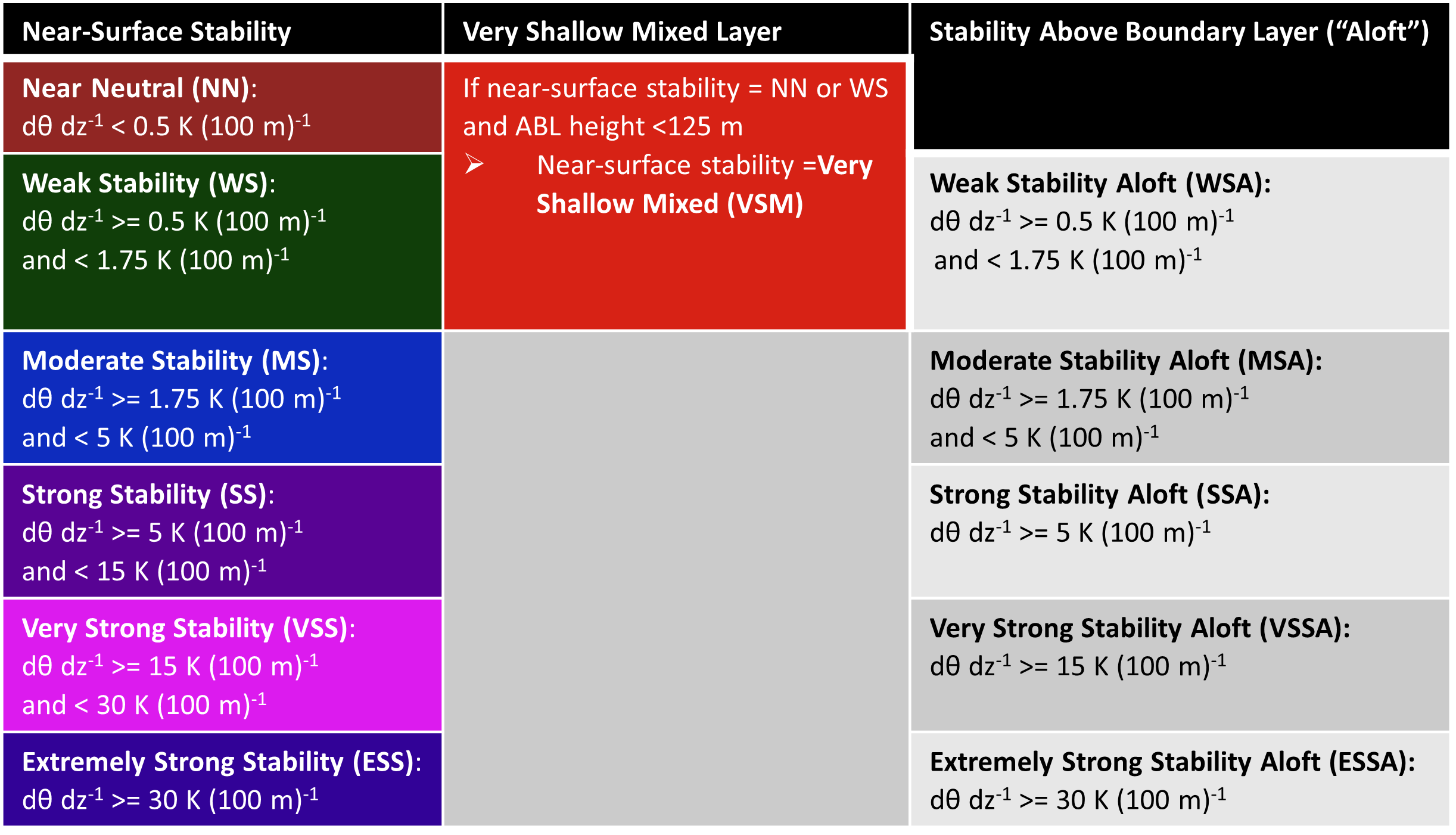
Six near-surface stability regimes were defined (Table 2, left column) based on the potential temperature gradient between 20 and 50 m a.g.l., as this depth captures the near-surface conditions while avoiding measurement errors below 20 m. The near-surface stability regimes range from near neutral (NN; K per 100 m) to extremely strongly stable (ESS; K per 100 m). Various thresholds to distinguish near-neutral (NN), weak (WS), moderate (MS), strong (SS), very strong (VSS), and extremely strong (ESS) stability were evaluated, and the thresholds listed in Table 2 were found to best separate meaningful differences in near-surface stability across all five sites. These thresholds were also evaluated and found to be appropriate in a separate study based on profiles observed over Arctic sea ice as part of the MOSAiC expedition (Jozef et al., 2023). It is also important to note that the NN regime with potential temperature gradients less than 0.5 K per 100 m may include some negative potential temperature gradients; thus convective conditions, while rare in the Antarctic, can occur with strong radiative heating during the austral summer or advection of cold air over a relatively warmer surface.
It was also noted that many of the SOM patterns were characterized by a layer of stronger stability above weaker stability near the surface, which was also noted by Dice and Cassano (2022) at McMurdo. Therefore, the stability above the boundary layer is also used to define the overall stability regime (Table 2). This requires identifying the top of the boundary layer, which is done following Jozef et al. (2022) by using profiles of the bulk Richardson number. The bulk Richardson number is defined as the approximation of the ratio of buoyant turbulence production, or suppression, to mechanical generation of turbulence by wind shear. A critical bulk Richardson number indicates the point at which turbulence cannot be sustained (Stull, 1988). The boundary layer height is defined as the point in the profile where the bulk Richardson number exceeds a critical value of 0.5 and remains above that critical value for at least 20 m consecutively.
where, in Eq. (1), g is the acceleration due to gravity, θ is potential temperature, U is the zonal wind, and V is the meridional wind; Δ indicates the change in variables over the change in altitude (Δz, 5 m); and the overbar indicates the mean potential temperature over the change in altitude (Δz).
Aloft stability regimes were determined with the same potential temperature gradient thresholds as were used for the near-surface stability regimes (Table 2). The maximum potential temperature gradient above the boundary layer height and below 500 m was used to identify the aloft stability regimes. Aloft stability regimes were applied to any potential temperature gradient profile with a greater stability aloft compared to the near-surface stability of that profile. No aloft stability regime is applied for cases with the strongest stability near the surface.
Boundary layer stability regimes were also defined based on the depth of the boundary layer. In analyzing all the boundary layer profiles it was found that there was a clear distinction between a group of NN and WS regimes with boundary layer heights less than 125 m and NN and WS regimes with boundary layer heights much greater than 125 m. Thus, a very shallow mixed (VSM) stability regime was defined to distinguish these cases, specifically for the NN and WS regimes with boundary layer depths less than 125 m.
The near-surface and aloft stability regimes, along with the VSM regimes, were combined into an overall stability regime, as listed in Table 3. For example, a profile identified as having near-neutral stability near the surface with strong stability above the boundary layer would be identified as near neutral, strong stability aloft, or NN-SSA. Thus, we end up with “stability groupings” with the same near-surface stability for multiple regimes but with varying stability aloft. One example of these groupings is the following: NN (near neutral), NN-WSA (near neutral, weak stability aloft), NN-MSA (near neutral, moderate stability aloft), and NN-SSA (near neutral, strong stability aloft; Table 3). The boundary layer stability regimes defined here are then applied to the patterns in the SOMs to show how this definition scheme applies to the range of potential temperature gradient profiles originally identified in the SOM, which was used to inform the development of the boundary layer stability regime definitions.
Table 3Boundary layer regime acronyms and color codes. On the left is the color and acronym used to represent each of the 20 stability regimes in figures and tables throughout this paper, and the full regime name is spelled out on the right. The basic near-surface stability regimes are denoted in bold font.
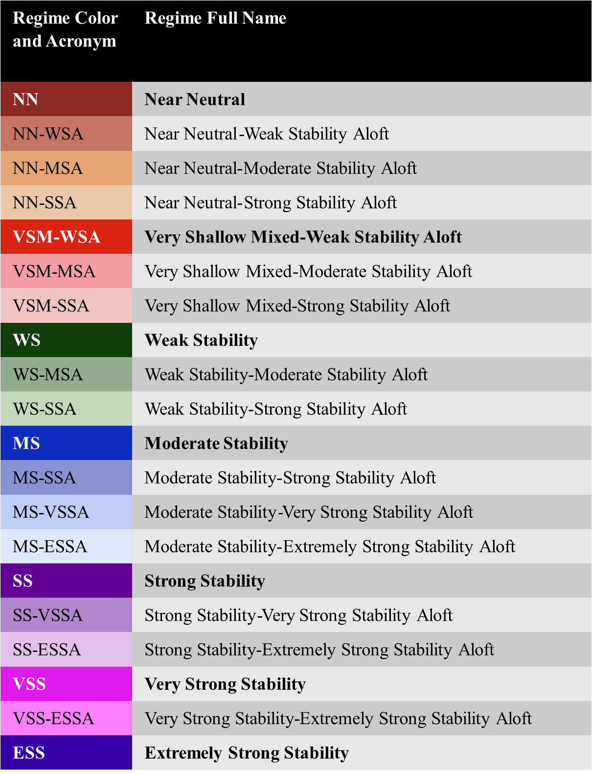
Regimes where no increased stability aloft is present (NN, WS, MS, SS, VSS, or ESS) as well as VSM-WSA will be referred to as “basic near-surface stability regimes”. The reasoning for including VSM-WSA in the basic near-surface stability regimes is that this regime is defined by both stability and boundary layer depth. The VSM regime is derived from the same conditions that define the NN and WS regimes, but in the VSM regime, a much shallower boundary layer exists (less than 125 m). The WSA in this regime is consistent with the potential temperature gradient that defines the VSM regime as a whole and is thus considered part of the basic near-surface stability regimes. Each stability grouping is identified by a distinct color (Table 3; NN – brown, VSM – red, WS – green, MS – blue, SS – purple, VSS – pink, ESS – indigo), in which the darkest color is the basic near-surface regime (no increased stability aloft), with decreasing color intensity as stability aloft in that regime grouping increases.
2.2.3 Clear- and cloudy-regime classification
As mentioned in the Introduction, wintertime boundary layer stability in the polar regions is often described as being made up of two regimes, which differ based on the presence or absence of clouds and the associated differences in downwelling longwave radiation. This two-regime system is often defined as a “clear regime”, with low values of downwelling longwave radiation, strong surface radiative cooling, and strong stability, and a “cloudy regime”, with enhanced downwelling longwave radiation, surface warming and decreased near-surface stability (Phillpot and Zillman, 1970; Stone and Kahl, 1991; Solomon et al., 2023). Here, we will assess how the frequency of the 20 boundary layer regimes (Table 2) relate to the more commonly defined clear (strongly stable) and cloudy (weakly stable) regimes to evaluate the use of this more nuanced view of the relationship between boundary layer stability and cloud cover.
To determine the conditions with which the boundary layer regimes defined in Table 2 occur, we follow the approach of Solomon et al. (2023) that used net longwave radiation observations taken over the Arctic sea ice during the MOSAiC expedition to define clear and cloudy conditions. They found that during the winter there was a bimodal distribution of net longwave radiation. The minimum in frequency between the two peaks of this distribution was used to define clear and cloudy states, which were found to have distinct distributions of downwelling longwave radiation (Solomon et al., 2023). Following Solomon et al. (2023) this analysis will be completed only in the winter season.
PDFs of wintertime net longwave radiation are calculated at the five study sites (Figs. S1 to S5 in the Supplement) to determine if bimodal distributions of net longwave radiation are found at coastal and interior Antarctic sites, like what was found in the Arctic. Then, as in Solomon et al. (2023), we determine if distinct distributions in downwelling longwave radiation are present, which serve as a proxy for clear (small values of downwelling longwave radiation) or cloudy (large values of downwelling longwave radiation) conditions. Solomon et al. (2023) used the minima in the net longwave radiation PDF as a threshold to define clear and cloudy regimes. In this study, we define an overlap ratio (defined below) that quantifies how distinct the distributions of downwelling longwave radiation are for a given net longwave radiation threshold used to separate clear and cloudy states. For the identified net longwave radiation threshold, we create two PDFs of downwelling longwave radiation (Figs. S1 to S5) based on the subset of observations corresponding to net longwave radiation values above (cloudy) or below (clear) the net longwave radiation threshold. Using the two downwelling longwave radiation PDFs, we determine the total number of clear cases and cloudy cases and the number of coincident cases where the clear and cloudy PDFs overlap. The overlap ratio is calculated as the number of overlapping cases divided by the total number of clear and the total number of cloudy cases, and the final overlap ratio is the maximum of these two ratios. This overlap ratio quantifies how much overlap exists between the clear and cloudy downwelling longwave radiation PDFs, and distinct clear and cloudy PDFs are characterized by low overlap ratios. The overlap ratio is calculated for each value of net longwave radiation (from the minimum to the maximum observed), at 1 W m−2 intervals, at each site. The minimum overlap ratio at each site, from the calculations every 1 W m−2, defines the net longwave radiation threshold identifying the most distinct distributions of downwelling longwave radiation for clear and cloudy cases. It generally corresponds to within a few watts per square meter of the minimum in the bimodal PDF of net longwave radiation (vertical black line in Figs. S1 to S5 in the Supplement). The dates and times corresponding to the clear and cloudy states were used to determine the frequency of boundary layer stability regimes for the two states.
3.1 South Pole
At a high-plateau continental-interior site such as South Pole, it is expected that strong stability will be present throughout much of the year (Phillpot and Zillman, 1970; Comiso, 1994; Hudson and Brandt, 2005; Zhang et al., 2011). The SOM in Fig. 2 shows the range of potential temperature profiles (anomaly and gradient) across 16 years of radiosonde observations at South Pole, as well as the stability regime (colored outline and label in the top left of each pattern) corresponding to the mean profiles in each SOM pattern. The left side of the SOM is dominated by the strongest stability patterns, and stability decreases from left to right, with the weakest stability patterns in the upper right corner. Potential temperature gradients of more than 5 K per 100 m in nearly all of the SOM-identified patterns in Fig. 2, with many greater than 15 K per 100 m and some even greater than 30 K per 100 m, show that strong stability is in fact common at this site. Potential temperature gradients in excess of 15 K per 100 m, corresponding to our VSS regime (Table 2), are rarely observed outside of the interior of Antarctica, over the Greenland ice sheet, or over Siberia in the Arctic (Zhang et al., 2011). Potential temperature gradients of less than 1.75 K per 100 m, corresponding to NN or WS regimes, occur only in patterns 6, 12, and 18 in the upper right of the SOM, emphasizing the dominance of strong stability at South Pole.
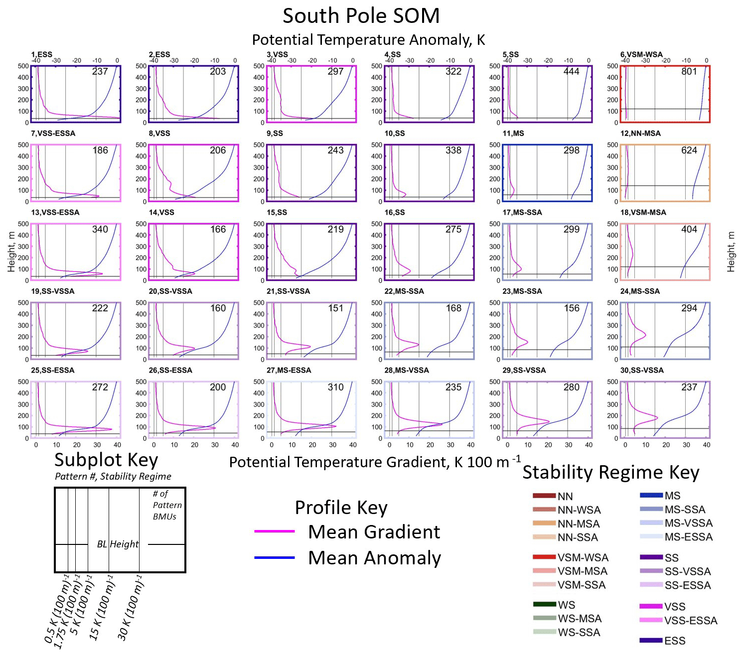
Figure 2Profiles of the mean potential temperature gradient (pink line, bottom axis) and mean potential temperature anomaly (blue line, top axis) calculated from the BMUs that map to each SOM pattern from 20 to 500 m a.g.l. at South Pole. BL: boundary layer.
The height of the maximum potential temperature gradient within the profile varies across the SOM, often being located very close to the surface, as in the top left corner of the SOM, but sometimes the maximum gradient is located above a layer of decreased stability near the surface, as is in the bottom two rows of the SOM. These SOM patterns represent conditions with moderate or strong near-surface stability capped by enhanced stability aloft (strong stability aloft, SSA; very strong stability aloft, VSSA; extremely strong stability aloft, ESSA).
The SOM for South Pole (Fig. 2) shows the boundary layer height for each SOM pattern, in addition to showing potential temperature gradient and anomaly profiles. The boundary layer depth rarely exceeds 100 m across the SOM and is very shallow (less than 50 m a.g.l.) for the SS, VSS, and ESS cases present throughout much of the SOM. The boundary layer depth increases in the MS cases in the bottom right corner of the SOM (approximately 100 m) and is deepest in the NN and VSM cases in the top right of the SOM (just above 100 m).
As mentioned in Sect. 2.2.2, the stability regime for each individual radiosonde profile was identified to allow for comparison of regime frequencies across all five sites. Annual and seasonal stability regime frequencies at South Pole are shown in Fig. 3. When analyzing the frequency of boundary layer stability regimes on an annual basis (Fig. 3, left panel) the strongest near-surface stability regimes (SS, VSS, and ESS) are most common, occurring 58.5 % of the time cumulatively. This observation is consistent with what is seen in the SOM, where most of the profiles are SS, VSS, and ESS regimes. For the weaker stability regimes (NN, VSM, and WS) the most common types of these regimes are the ones with enhanced stability aloft, indicating that most of the time when weak stability is present near the surface moderate or strong stability remains aloft. Regardless of where strong stability occurs in the profile (near the surface or aloft), strong stability, very strong stability, and extremely strong stability occurs 85.1 % of the time annually at South Pole, indicating that this location is dominated by the strongest stability classes.
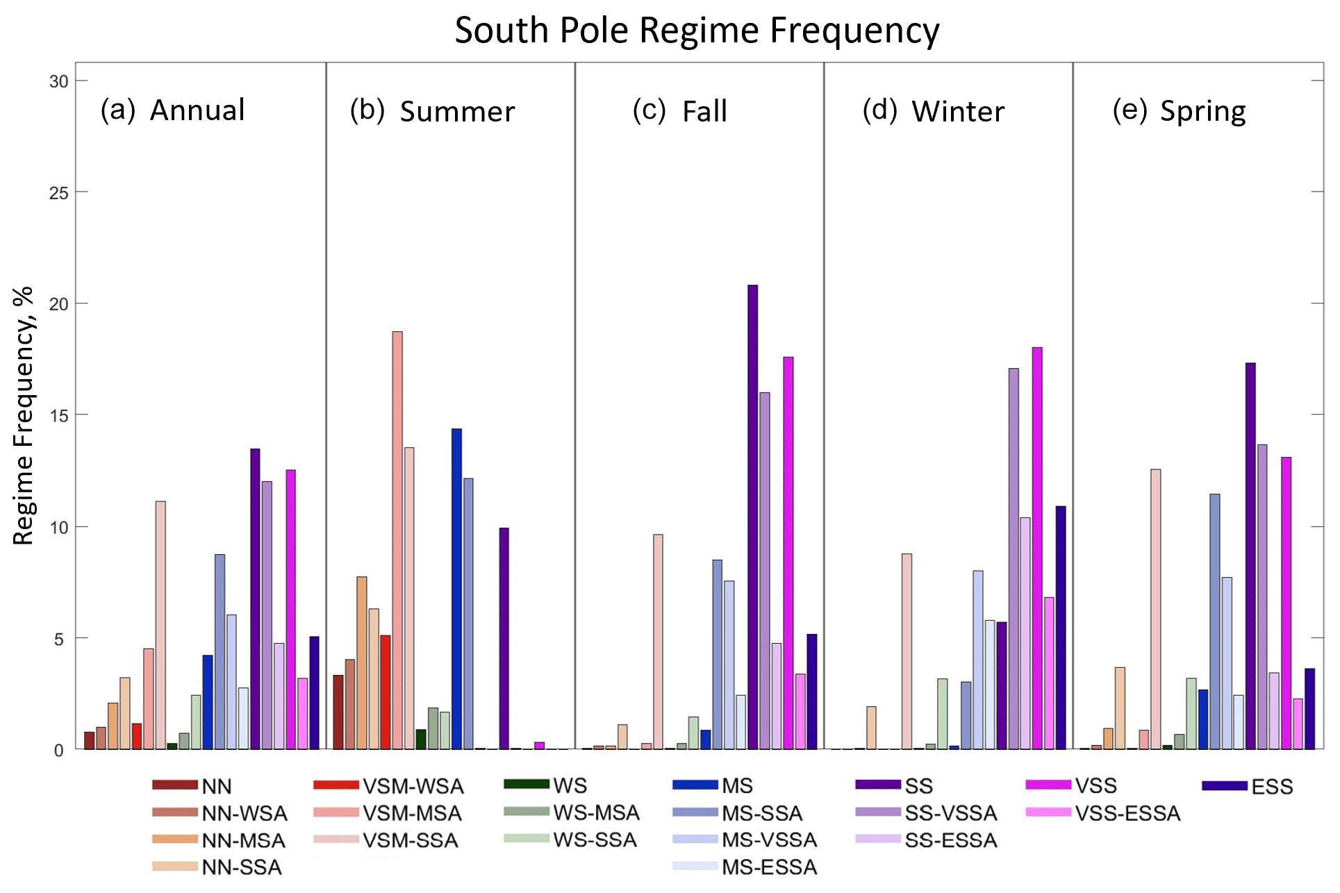
Figure 3Percentage of observations corresponding to each boundary layer stability regime observed at South Pole (a) annually and (b–e) seasonally (summer, fall, winter, and spring). The regimes for the annual and seasonal plots are arranged with increasing stability from left to right in each panel, and the order of the stability regimes in each panel corresponds to the order of the regimes, from top to bottom and left to right in the colored key at the bottom.
Seasonally there is a clear difference in regime frequencies between summer (DJ) and the other three seasons. In the summer, the weakest near-surface stability regimes (NN and VSM) account for most summer cases (58.7 %), although these are often with enhanced stability aloft. Despite the sun being continuously above the horizon during the summer, a high frequency of the MS and SS regimes (36.8 %) still occurs. WS regimes are very rare (4.5 %), along with the VSS and ESS regimes, which almost never occur at this time of year. In the winter (MJJA), SS, VSS, and ESS regimes dominate, occurring 68.9 % of the time, while NN and VSM occur only 10.7 % of time, and WS and MS cases make up the remainder of stability regimes observed in the winter (3.4 % and 16.9 %, respectively). Interestingly, the few NN, VSM, and WS cases in the winter all have strong stability aloft (SSA), indicating that even when the weakest stability regimes occur at the surface, strong stability is still present just above the boundary layer. The frequency of stability regimes in the transition seasons (fall, FMA; spring, SON) largely mirrors the frequency of stability regimes in the winter, again with the observation that the NN, VSM, and WS cases in the fall and spring almost always have strong stability aloft (SSA).
3.2 Dome C
Dome C is another high-plateau continental-interior site where strong stability persists throughout much of the year (King and Turner, 1997; Andreas et al., 2000). This can be seen in the Dome C SOM in Fig. 4, where, like South Pole, most of the SOM-identified profiles exhibit potential temperature gradients in excess of 5 K per 100 m and many are greater than 15 K per 100 m. The left four columns of the SOM are all stability regimes of SS or stronger (greater than 5 K per 100 m), and stability decreases from left to right with the weakest stability patterns in the upper right corner (less than 1.75 K per 100 m). The height of the maximum potential temperature gradient within the profile changes across the SOM, with the maximum stability observed at the surface in the upper left profiles and the height of this maximum stability increasing to the bottom right of the SOM, although the strongest stability usually occurs near the surface in most of the SOM patterns.
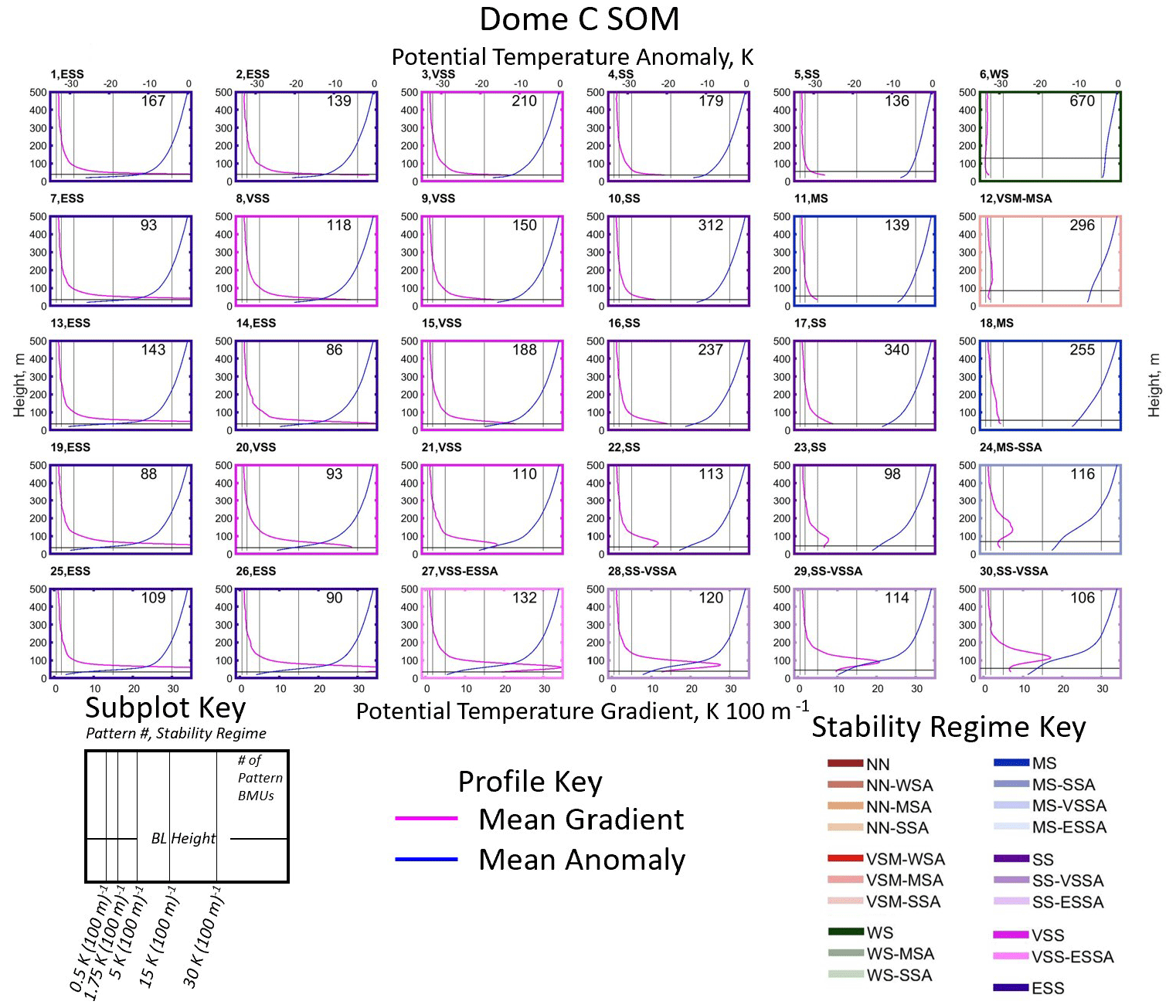
Figure 4Profiles of the mean potential temperature gradient (pink line, bottom axis) and mean potential temperature anomaly (blue line, top axis) calculated from the BMUs that map to each SOM pattern from 20 to 500 m a.g.l. at Dome C.
The boundary layer height is less than 50 m across most of the SOM and only increases when stability decreases, such as in the bottom right, where stability is moderate and the boundary layer height is about 75 m, and in the top right, where stability is weak and the boundary layer height is around 100 m. In general, these are still very shallow boundary layers, even in the weaker stability patterns, compared to other locations across the planet, where the height of the boundary layer can exceed 1000 m (Stull, 1988). Both at South Pole and Dome C strong, near-surface stability suppresses most of the mechanically generated turbulence, resulting in very shallow (typically less than 75 m) boundary layers. However, shallow boundary layers at both sites also occur in the upper right portions of the SOM where relatively weak stability exists, indicating that near-surface turbulent mixing is still confined to the lowest part of the atmosphere (less than 150 m).
The frequency of occurrence of each stability regime at Dome C is shown in Fig. 5. On an annual basis, SS, VSS, and ESS regimes occur most frequently (73.6 %), while the weaker stability regimes of NN, VSM, and WS only occur 13.5 % of the time. This is comparable to the range of stability regimes seen in the SOM, where these types of weaker stability regimes occur very rarely and SS, VSS, and ESS regimes dominate across most of the SOM. A strong seasonal cycle emerges, with the weaker stability regimes dominant in the summer and the strongest stability regimes dominant in the winter. The summer season is largely characterized by NN, VSM, and WS regimes (61.4 %), as well as MS regimes (31.1 %). In the summer, SS, VSS, and ESS regimes occur only 7.5 % of the time, indicating the rarity of strong stability at this time of year. In the winter, SS, VSS, and ESS regimes occur almost exclusively (96.7 %), while all the other regime groupings (VSM, NN, WS, and MS) occur very rarely (3.3 %). It is also interesting that the dominant regimes in the winter are solely the basic near-surface stability regimes of SS, VSS, and ESS, and increased stability aloft in these regimes occurs much less frequently, indicating that during the winter the strongest stability occurs at the surface most of the time, with infrequent cases of weakened stability near the surface and enhanced stability aloft. The frequency of stability regimes in the transition seasons (fall and spring) is also dominated by stronger stability regimes (SS, VSS, and ESS), although with slightly lower frequencies than in the winter, with these regimes occurring 83.7 % and 76.9 % of the time in the fall and spring, respectively. The weakest stability regimes (VSM, NN, and WS) occur rarely (4.6 % and 4.9 % of the time in the fall and spring, respectively), while the MS regime occurs 11.7 % and 15.7 % of the time in the fall and spring, respectively. In comparison to the summer and winter, the transition seasons behave more like the winter season when it comes to regime frequency, with most regimes showing strong stability.
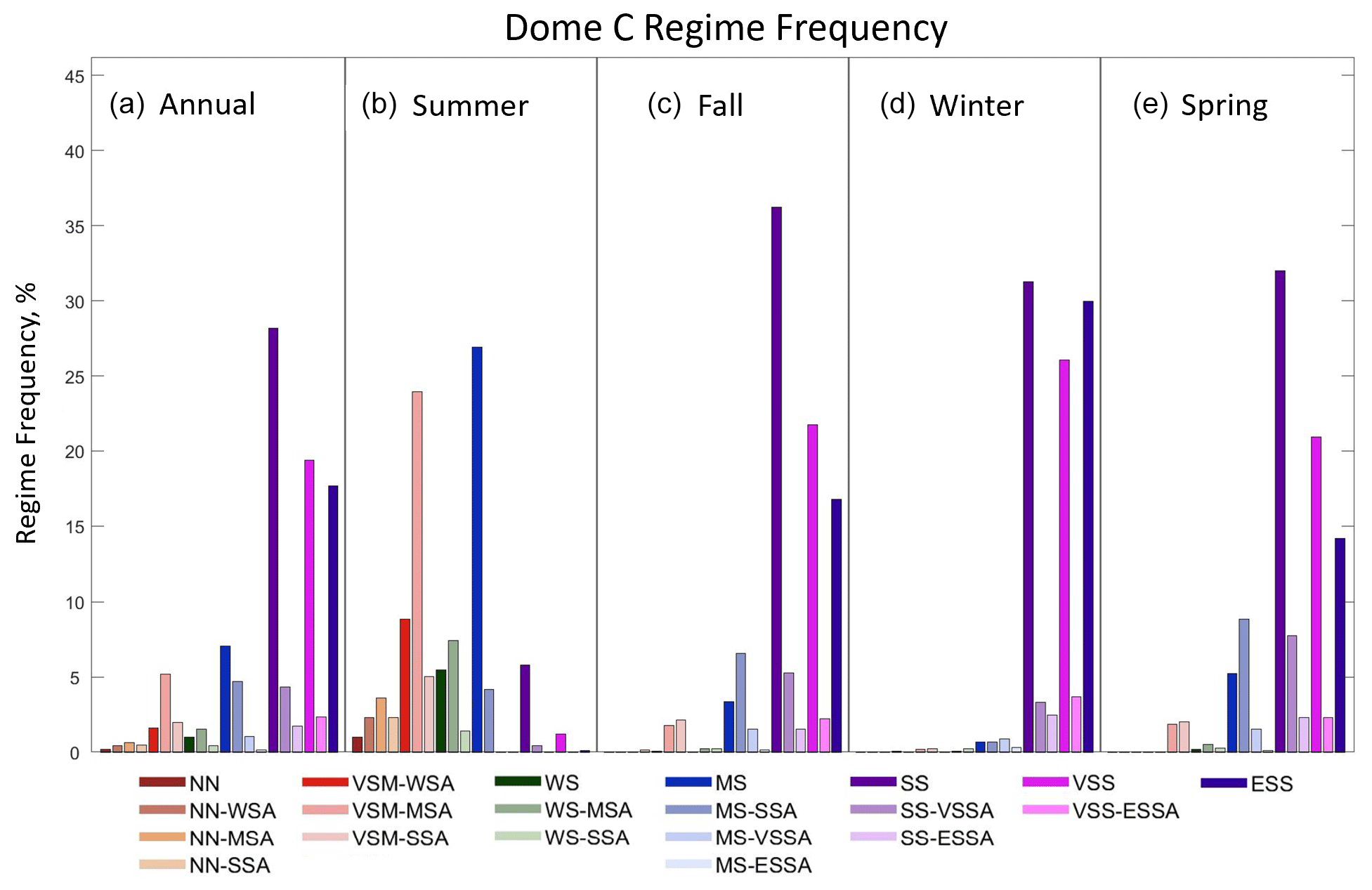
Figure 5Percentage of observations corresponding to each boundary layer stability regime observed at Dome C (a) annually and (b–e) seasonally (summer, fall, winter, and spring). The regimes for the annual and seasonal plots are arranged with increasing stability from left to right in each panel, and the order of the stability regimes in each panel corresponds to the order of the regimes, from top to bottom and left to right in the colored key at the bottom.
3.3 McMurdo
So far, two continental-interior sites, South Pole and Dome C, have been analyzed, and now the coastal sites, McMurdo, Neumayer, and Syowa, will be analyzed. In comparison to the continental interior, coastal locations are more exposed to the impacts of cyclonic activity, increased cloud cover and moisture, and warmer surface temperatures and weaker inversions (Phillpot and Zillman, 1970; Cassano et al., 2016). Given these previous observations, it is expected that weaker stability will be present at the coastal sites compared to the near-constant state of strong stability observed at the colder continental-interior sites described above.
Stability profiles at McMurdo identified by the SOM span a range from the NN to SS regimes, as seen in Fig. 6. Stability in the SOM increases from left to right, with the weakest stability patterns in the top left and strongest stability patterns in the bottom right. In addition to this gradient in stability across the SOM, the height of the strongest stability increases from the surface in the bottom rows of the SOM to above a near-surface layer of weaker stability in the top middle of the SOM. Most of these patterns with enhanced stability aloft exhibit moderate or strong stability (MSA or SSA, respectively) above a layer of weaker stability. Two-thirds of the SOM patterns exhibit potential temperature gradients less than 1.75 K per 100 m, corresponding to a stability of WS or weaker, and only five patterns on the right side of the SOM (patterns 12, 18, 23, 24, and 30) exhibit strong stability with gradients greater than 5 K per 100 m. It can also be seen that the height of the boundary layer increases from the bottom right (approximately 50 m) to the top left (approximately 200 m) as stability decreases and the height of the maximum stability increases in the profile.
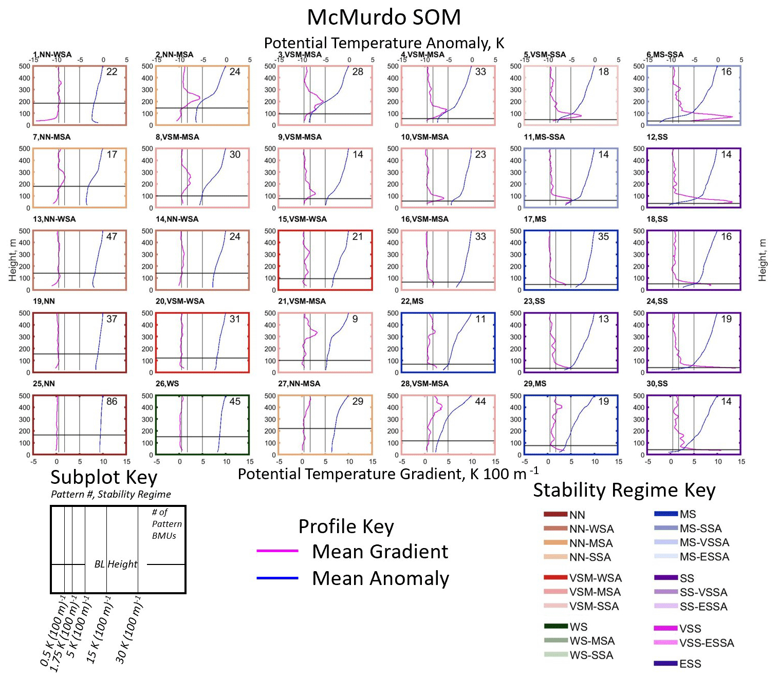
Figure 6Profiles of the mean potential temperature gradient (pink line, bottom axis) and mean potential temperature anomaly (blue line, top axis) calculated from the BMUs that map to each SOM pattern from 20 to 500 m a.g.l. at McMurdo.
Considering regime frequencies on an annual basis, the NN and VSM regimes are most common (68.6 %), followed by the MS and SS regimes (24.9 %). The summer season is dominated by the NN and VSM regimes (91.2 %), and the WS, MS, and SS regimes occur only 8.8 % of the time. This distribution of stability is consistent with increased radiative forcing and previous observations of weaker stability in the summer compared to other seasons at a site approximately 100 km from McMurdo (Cassano et al., 2016). In the winter, when it would be expected that strong stability would be dominant, only about half of the time regimes with a stability of MS and greater occur (46.4 %), while regimes with a stability of WS and weaker occur just over half of the time (53.6 %). However, when the regimes with a stability of WS and weaker occur, moderate or strong stability aloft (MSA and SSA, respectively) is usually present (84 % of NN, VSM, and WS cases have MSA or SSA), indicating that even when weaker stability occurs near the surface, moderate or stronger stability is present just above the boundary layer. In the transition seasons, cases of MS and stronger occur 23.9 % of the time in the fall and 28.2 % of the time in the spring. NN and VSM cases cumulatively occur 73.3 % of the time in the fall and 67.3 % in the spring, while WS cases are largely absent. In the VSM regime grouping, the MSA and SSA regimes are most common, with the WSA regime occurring less frequently in comparison in both the spring and the fall. In the NN regime grouping, the frequency of occurrence decreases with increasing stability aloft in the fall and is more consistent across the WSA, MSA, and SSA regimes in the spring. This indicates that in the fall, it is more common for NN cases to have weak rather than strong stability aloft, similar to that observed in the summer and opposite to that in the winter.
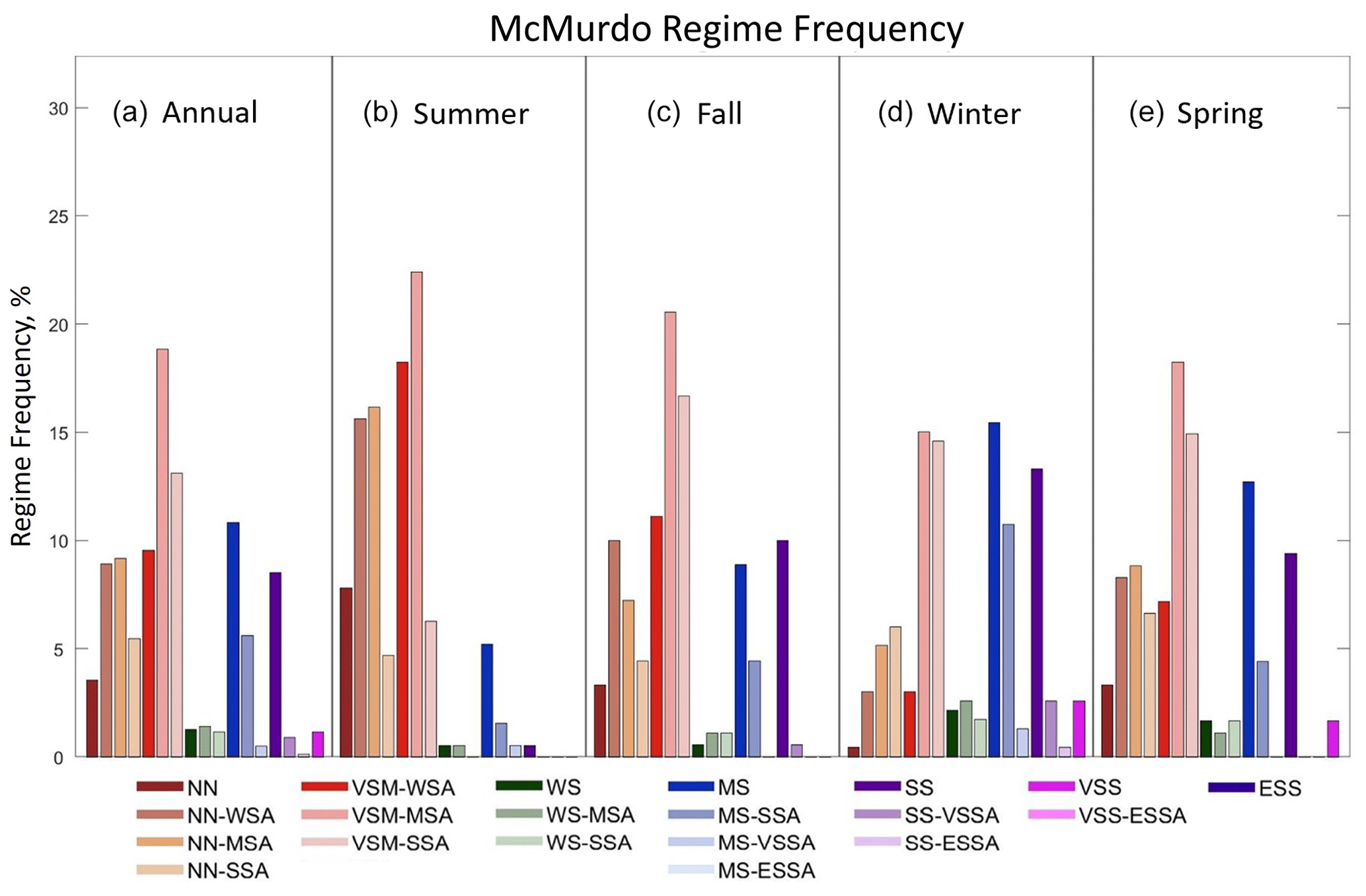
Figure 7Percentage of observations corresponding to each boundary layer stability regime observed at McMurdo (a) annually and (b–e) seasonally (summer, fall, winter, and spring). The regimes for the annual and seasonal plots are arranged with increasing stability from left to right in each panel, and the order of the stability regimes in each panel corresponds to the order of the regimes, from top to bottom and left to right in the colored key at the bottom.
3.4 Neumayer
Neumayer is a coastal site located near sea level, heavily influenced by large-scale cyclonic activity (Silva et al., 2022) and where the proximity of sea ice and open ocean can affect boundary layer stability throughout the year (Silva et al., 2022). Stability regimes at Neumayer span a range from the NN to VSS regimes, as seen in the SOM in Fig. 8. Generally, stability decreases from left to right across the SOM. Stability on the left side of the SOM decreases from the top to the bottom of the SOM, with the strongest stability regimes in the top left. On the right side of the SOM, deep near-neutral or weak stability patterns occur at the top of the SOM, with patterns characterized by increasing stability aloft occurring towards the bottom of the SOM. This SOM shows two general modes of stability split by a diagonal from the bottom left to top right, with the portion to the right of this diagonal characterized by the NN, VSM, and WS regimes and the portion to the left characterized by the MS, SS, and VSS regimes. The boundary layer height at Neumayer increases from the left side of the SOM, where very shallow boundary layers exist (less than 50 m) with strong stability, to the top right, where the boundary layer height increases to above 200 m.

Figure 8Profiles of the mean potential temperature gradient (pink line, bottom axis) and mean potential temperature anomaly (blue line, top axis) calculated from the BMUs that map to each SOM pattern from 20 to 500 m a.g.l. at Neumayer.
On an annual basis, the NN and VSM regime groupings are most common (52.8 %), and the MS and SS (37.2 %) regimes occur slightly less frequently at Neumayer (Fig. 9). The WS regime grouping occurs 8.4 %, while the VSS and ESS regimes are rare and occur only 1.6 % of the time throughout the year. The summer season is dominated by the NN and VSM regimes (74 %). The WS (6.1 %), MS (14 %), and SS (5.9 %) regimes are much less common in comparison. In the VSM and NN regime groupings, regimes with weak stability aloft (WSA) are more common than those with stronger stability aloft (MSA and SSA). In the winter, regimes with a stability of MS or greater are most common (60.1 %), while regimes with weaker stability, WS (12.2 %), VSM (13 %), and NN (14.7 %), occur less frequently. Further, many of the weaker stability regimes present in the winter are those with increased stability aloft, especially MSA and SSA, indicating that moderate or stronger stability is frequently present either near the surface or aloft in the winter (89.5 % of the time), whereas in the summer these moderate or strong stability cases (either at the surface or aloft) cumulatively occur 50.7 % of the time. In the fall, the NN and VSM cases (47.9 %) and cases of MS and stronger (44.6 %) occur with almost equal frequency, unlike in the summer when the NN and VSM cases are dominant and winter when the cases of MS and stronger are dominant. In the spring, the VSM and NN cases (59.6 %) occur more frequently than the cases of MS and stronger (32.9 %), which is more similar to the distribution of regimes in the summer, when weaker stability regimes dominate.
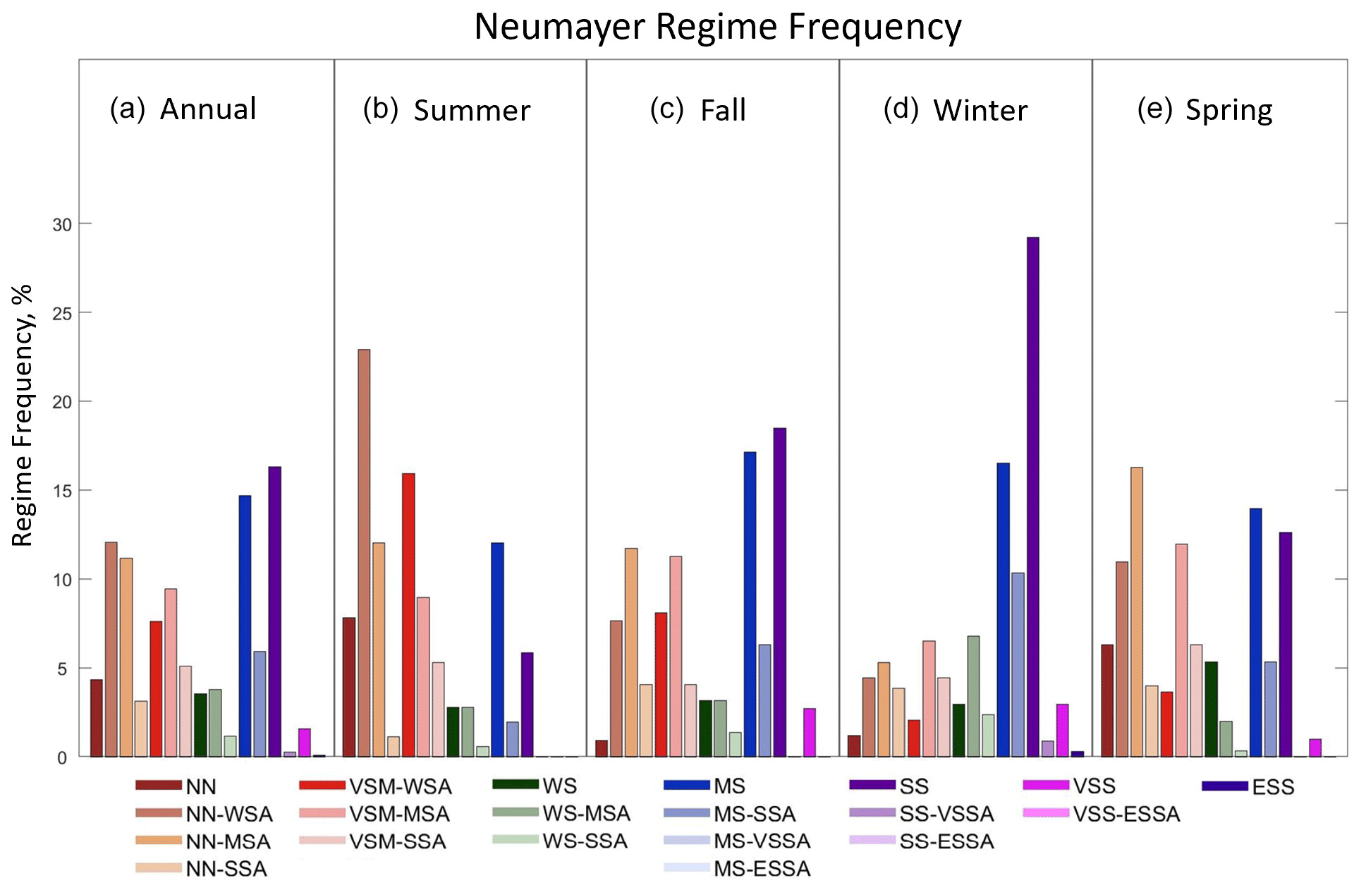
Figure 9Percentage of observations corresponding to each boundary layer stability regime observed at Neumayer (a) annually and (b–e) seasonally (summer, fall, winter, and spring). The regimes for the annual and seasonal plots are arranged with increasing stability from left to right in each panel, and the order of the stability regimes in each panel corresponds to the order of the regimes, from top to bottom and left to right in the colored key at the bottom.
3.5 Syowa
Syowa is a coastal site near sea level, impacted by cyclonic activity and by katabatic winds from the continental interior (Murakoshi, 1958), which sometimes result in strong wind events (Yamada and Hirasawa, 2018). Stability at Syowa spans a range from the NN (top left corner of SOM) to SS (bottom right corner of SOM) regimes, as seen in the SOM in Fig. 10. Stability generally increases from left to right and top to bottom across the SOM. The height of the maximum potential temperature gradient is near the surface on the far-right side of the SOM and increases to approximately 300 m in the bottom left. Shallow boundary layers associated with the strong stability patterns in the bottom right increase in height to the top left, where near-neutral conditions extend through a deeper, 200 m boundary layer.
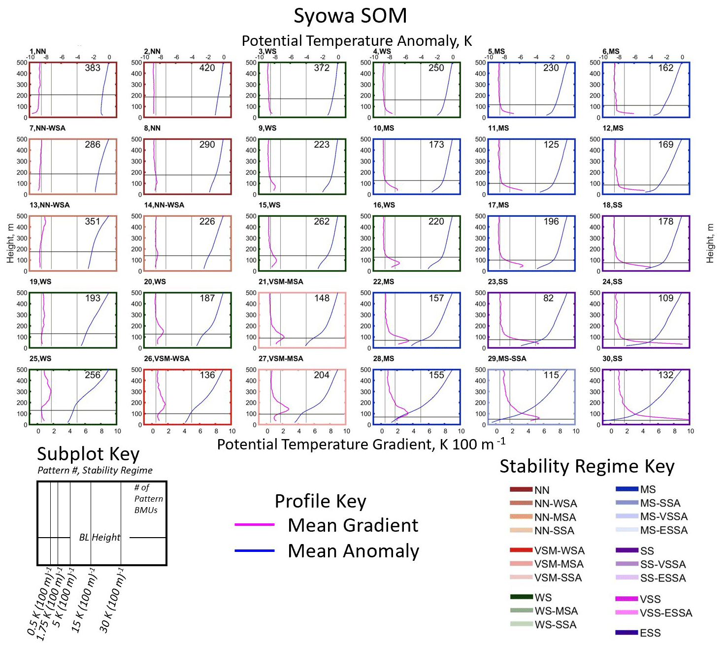
Figure 10Profiles of the mean potential temperature gradient (pink line, bottom axis) and mean potential temperature anomaly (blue line, top axis) calculated from the BMUs that map to each SOM pattern from 20 to 500 m a.g.l. at Syowa.
The frequency of occurrence of each stability regime at Syowa, annually and seasonally, is shown in Fig. 11. On an annual basis, a mix of regimes are observed, mostly in the NN (21.8 %) and VSM (31.4 %) regime groupings, with enhanced stability aloft common. The WS regime (15.1 %) and MS regime (25.1 %) also occur frequently, on an annual basis, but enhanced stability aloft rarely occurs in these regime groupings. The strongest stability regimes (SS, VSS, and ESS) occur infrequently (6.8 %). These results indicate that near-neutral to moderate stability is most common at Syowa, while stronger stability is rare. The summer season is dominated by the NN and VSM regimes (71.5 %), while the WS regime occurs 11.4 % of the time and the MS regime occurs 15.3 % of the time. In all regime groupings in the summer, strong stability aloft (SSA) regimes are less common than weak or moderate stability aloft (WSA and MSA, respectively), which is reflective of the lack of strong stability regimes in general in this season. In the winter, MS and SS regimes (45.4 %) occur about as often as the NN and WS regimes (43.4 %), but MS is by far the most common individual regime in the winter (31 %). Regimes with increased stability aloft (MSA and SSA) are uncommon in the winter, except in the VSM regime grouping, and instead the basic near-surface stability regimes (without enhanced stability aloft) or WSA cases are more common. In the transition seasons, a variety of regimes occur with similar frequencies. In the fall the most common regime groupings are the VSM cases (34 %) followed by the NN cases (24.2 %) and the MS cases (20.4 %), and in the spring, the VSM (30.5 %) regimes are most common followed by MS (24.6 %) and NN (24.5 %) regimes that occur with nearly identical frequencies. In both seasons, like the summer and winter, MSA and SSA cases occur rarely, with WSA being more common when increased stability aloft is observed for a given regime grouping.
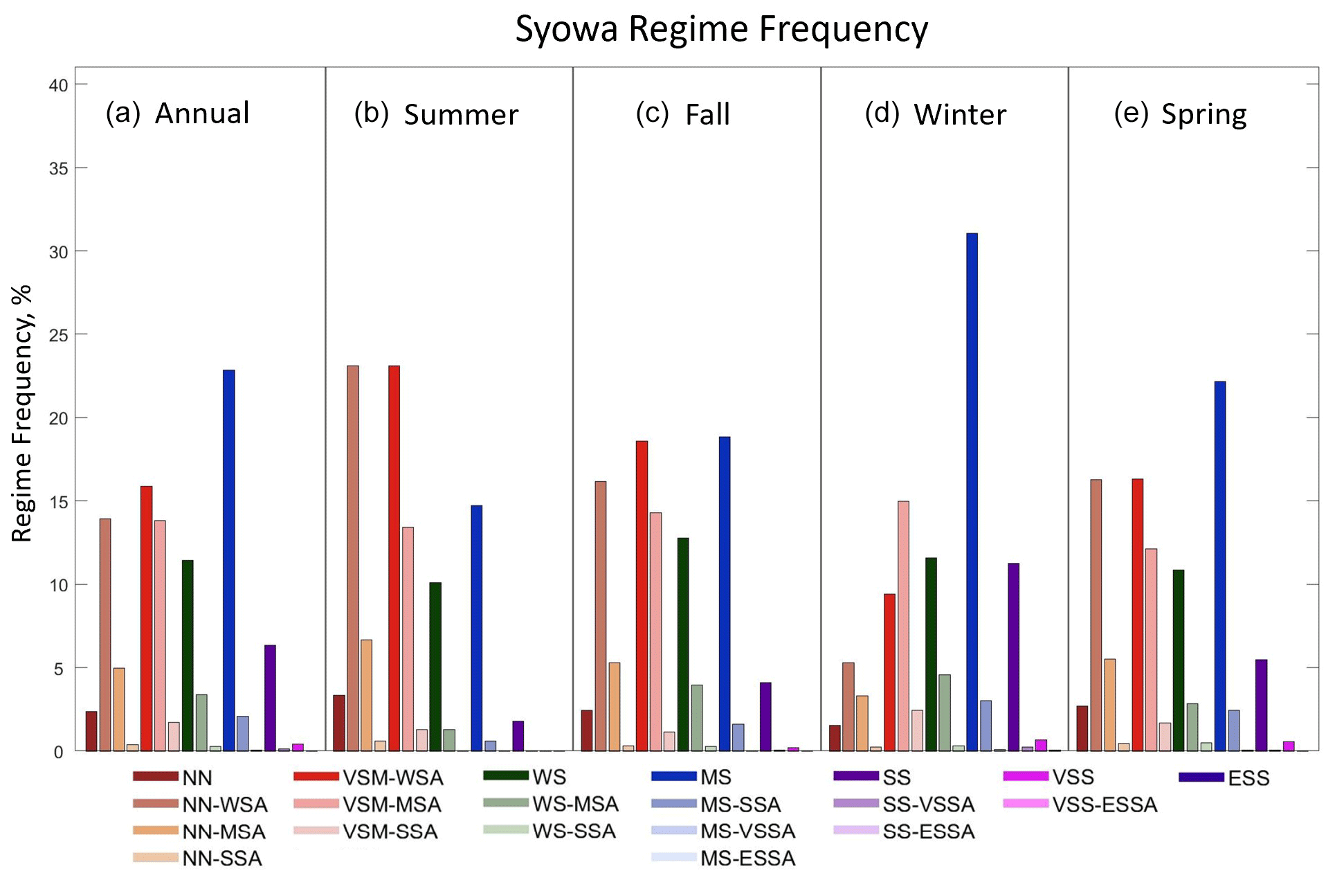
Figure 11Percentage of observations corresponding to each boundary layer stability regime observed at Syowa (a) annually and (b–e) seasonally (summer, fall, winter, and spring). The regimes for the annual and seasonal plots are arranged with increasing stability from left to right in each panel, and the order of the stability regimes in each panel corresponds to the order of the regimes, from top to bottom and left to right in the colored key at the bottom.
3.6 Stability regime frequencies for clear and cloudy conditions
As discussed in the Introduction and Methods, stability in the polar boundary layer is often described in the literature as a two-regime system, with cloudy states characterized by large values of downwelling longwave radiation and weak stability and clear states characterized by small values of downwelling longwave radiation and strong stability (Mahrt, 1998, 2014; Solomon et al., 2023). To determine if this two-regime description of boundary layer stability and cloud cover is observed in the Antarctic, a clear or cloudy attribution was given to each radiosonde profile based on the surface net longwave radiation value at the time of launch following the method described in Sect. 2.2.3, based on Solomon et al. (2023).
Solomon et al. (2023) found that the difference between cloudy and clear states in the Arctic could be defined by a threshold value of net longwave radiation marking the minimum in the PDF between two peaks in a bimodal distribution of net longwave radiation. PDFs of winter net longwave radiation at the five Antarctic sites analyzed in this paper are shown in Figs. S1 to S5. The PDFs for the two interior sites (Dome C and South Pole, Figs. S1 and S2) do not show a bimodal distribution, while the three coastal sites do (Figs. S3 to S5). The overlap ratio for the cloudy and clear downwelling longwave radiation PDFs for each site, as described in Sect. 2.2.3, further supports the lack of distinct cloudy and clear radiative states at the interior sites, with large values of this ratio (0.84 at South Pole and 0.91 at Dome C) indicating that there is no value of net longwave radiation that allows for a meaningful separation between cloudy and clear states with unique distributions of downwelling longwave radiation. The inability to find a distinction between the clear and cloudy states at the continental-interior sites may be related to the fact that previous studies have noted that the cold, dry atmosphere of the continental interior of Antarctica is conducive to high, optically thin ice clouds, rather than optically thick liquid or mixed-phase clouds which are lower and have higher near-surface radiative impacts (Morley et al., 1989; Town et al., 2005, 2007; Ganeshan et al., 2022). In contrast, the three coastal sites have overlap ratios of less than 0.5 (0.19 for McMurdo, 0.33 for Neumayer, and 0.46 for Syowa) for net longwave radiation threshold values that correspond closely to the minimum in the net longwave radiation PDF (Figs. S3 to S5), indicating that distinct downwelling longwave radiation distributions exist for cloudy and clear states at these sites. As such, we will evaluate the frequency of stability regimes for cloudy and clear conditions at the three coastal sites but not for the interior sites.
Figure 12 shows the frequency of each stability regime for cloudy (solid bars) and clear (hatched bars) cases for the three coastal sites: McMurdo, Neumayer, and Syowa. At McMurdo (Fig. 12a), the most obvious result is that the MS, SS, and VSS regimes occur much more frequently during the clear-sky state. This result is consistent with previous observations that clear skies allow for radiative cooling and the development of strong near-surface stability (Stone and Kahl, 1991; Hudson and Brandt, 2005). In contrast, the NN and WS regimes generally occur preferentially during cloudy conditions, also consistent with previous results that increased cloud cover reduces near-surface stability (Stone and Kahl, 1991; Hudson and Brandt, 2005). Interestingly, the VSM and NN-SSA regimes occur nearly equally regardless of cloud cover. This indicates that changes in downwelling longwave radiation related to varying cloud cover do not play a dominant role in the forcing of these regimes.
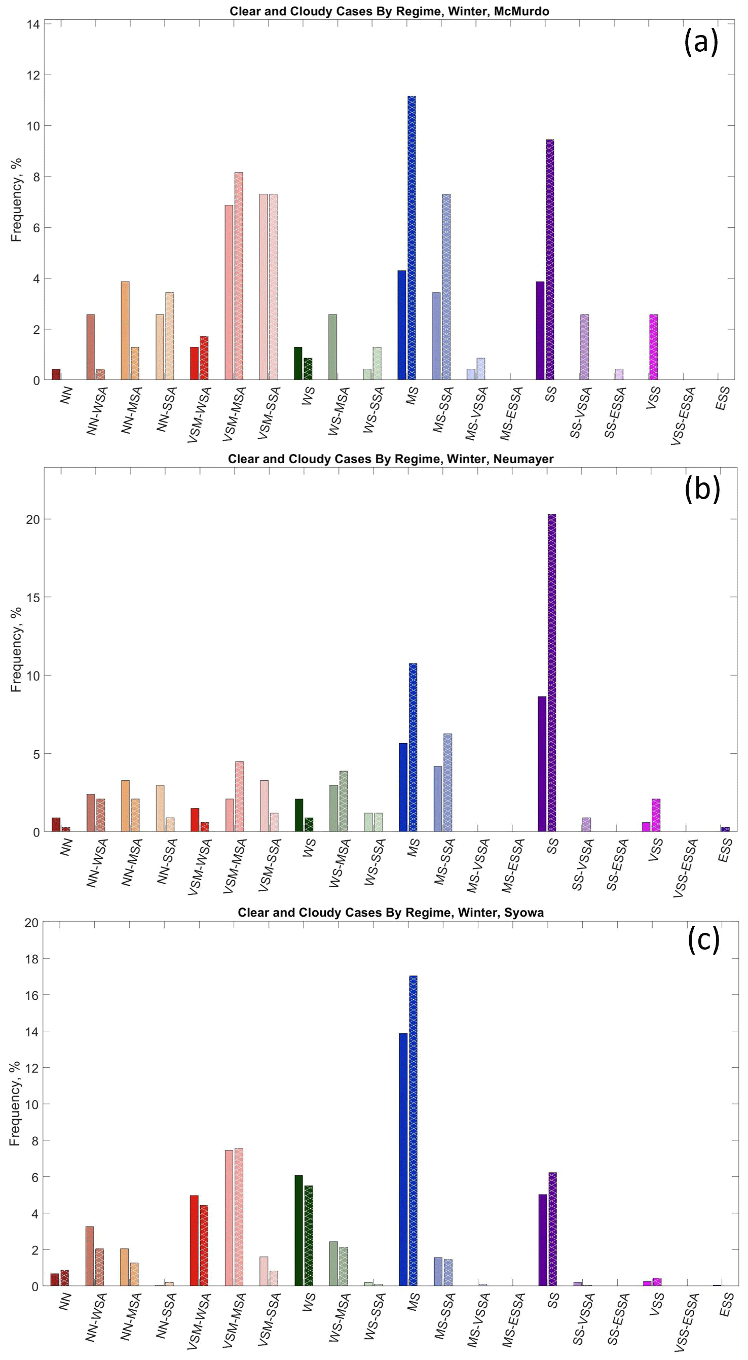
Figure 12The distribution of the various boundary layer stability regimes at (a) McMurdo, (b) Neumayer, and (c) Syowa split into cloudy (left, solid bars) and clear (right, hatched) observations in the winter season.
When examining the distribution for Neumayer (Fig. 12b), the SS regime is over twice as frequent during clear compared to cloudy conditions, as expected (Stone and Kahl, 1991; Mahrt, 1998, 2014; Solomon et al., 2023). The same is true for the VSS regime, and clear conditions are present for the singular ESS regime as well. The MS and MS-SSA regimes also occur more frequently with clear rather than cloudy conditions. The NN regimes usually occur with cloudy compared to clear conditions. The various VSM and WS regimes have occurrences where sometimes clear and sometimes cloudy periods are dominant. There are also VSM and WS regimes where they are roughly equal. This suggests that changes in downwelling longwave radiation associated with changes in cloud cover do not play a primary role in forcing the VSM or WS regimes to occur.
Finally, at Syowa (Fig. 12c), an interesting pattern emerges, where the frequency of most stability regimes is similar for both cloudy and clear conditions. This is surprising, given that previous studies have found weaker stability is favored by cloudy conditions and stronger stability is favored by clear conditions. This is not the case at Syowa and may indicate that changes in downwelling longwave radiation, associated with cloudy and clear conditions, do not exert a strong control on near-surface stability at this site.
SOMs have been used in the results presented above to identify the range of boundary layer stability profiles at two continental-interior and three coastal Antarctic sites (Figs. 2, 4, 6, 8, and 10). Based on the SOM analysis a quantitative boundary layer stability definition was developed and applied to classify the SOM patterns into unique stability regimes. While several studies have examined general trends in boundary layer stability at individual sites in Antarctica (Hudson and Brandt, 2005; Cassano et al., 2016; Silva et al., 2022) or estimated inversion strength empirically (Phillpot and Zillman, 1970), no known study has completed a widespread comparison of the range and seasonality of boundary layer stability across the continent.
The stability regimes present, as well as frequency of these regimes, differed between the continental-interior sites and the coastal sites. At the interior sites, South Pole and Dome C, strong stability patterns dominate the SOM, consistent with previous studies of near-surface stability on the polar plateau (Hudson and Brandt, 2005; King and Turner, 1997; Andreas et al., 2000); 27 of 30 patterns at South Pole (Fig. 2) and 28 of 30 patterns at Dome C (Fig. 4) have stability between MS and ESS, with potential temperature gradients in excess of 30 K per 100 m in several of the SOM profiles. Some of the SOM-identified profiles at these sites have weaker stability near the surface, with stronger stability aloft, and these patterns are more common at South Pole (Fig. 2, bottom two rows) than at Dome C (Fig. 4, bottom right corner). Finally, there are generally more VSS and ESS patterns in the Dome C SOM (left two columns) compared to the South Pole SOM (upper left corner), indicating stronger stability at this site, which was also observed by Hudson and Brandt (2005).
In contrast to the interior sites, at the coastal sites, McMurdo (Fig. 6), Neumayer (Fig. 8), and Syowa (Fig. 10), the SOM profiles are more evenly distributed across the NN, VSM, WS, MS, and SS profiles, with only one VSS profile and no ESS profiles. Across all three coastal sites, over half of the SOM-identified patterns have a potential temperature gradient less than 1.75 K per 100 m. These gradients occurred for only two or three patterns at Dome C and South Pole, respectively. This indicates more favorable conditions for weaker near-surface stability at coastal sites (Phillpot and Zillman, 1970; Cassano et al., 2016). This clearly distinguishes the boundary layer conditions of the continental-interior sites from those at the coastal sites, as also noted by Lettau and Schwerdtfeger (1967), Phillpot and Zillman (1970), Comiso (1994), Zhang et al. (2011), and Cassano et al. (2016). It is also important to note the common occurrence of enhanced stability above a layer of weaker near-surface stability in the SOMs for the coastal sites in comparison to the continental-interior sites. This phenomenon rarely occurs in the Dome C SOM, only in the bottom right corner (Fig. 4), as well as in the South Pole SOM, across the bottom two rows (Fig. 2), but it is also found across many of the SOM profiles for McMurdo (Fig. 6) and Neumayer (Fig. 8) and some of the SOM profiles for Syowa as well (Fig. 10).
The SOM analysis indicates a mean boundary layer depth being much shallower at Dome C (45 m) and South Pole (60 m) compared to the coastal sites (95 to 120 m). The strong near-surface stability that is almost always present at the continental-interior sites limits the depth and strength of turbulent mixing, while weaker stability at the coastal sites allows for stronger near-surface turbulence and thus increased boundary layer depths. This behavior of boundary layer depth is also observed by King and Turner (1997), who found shallow boundary layers in the continental interior, with boundary layer depth increasing towards the coasts. Pietroni et al. (2012) estimated the wintertime boundary layer height at Dome C using the bulk Richardson number and found it to be always below 150 m but usually less than 50 m, and Aristidi et al. (2005) found shallower boundary layer depths at Dome C (less than 50 m) compared to South Pole, consistent with our results.
To further summarize and compare the frequency of occurrence of boundary layer regimes (defined in Table 2) across the Antarctic continent, Fig. 13 and Table S1 in the Supplement provide a summary of the annual and seasonal characteristics of the near-surface stability and maximum stability below 500 m across all sites. Figure 13 shows the frequency of the near-surface stability regime groupings (e.g., all NN regimes, regardless of aloft stability; all VSM regimes, regardless of aloft stability) and the maximum stability present in the entire profile, either near the surface or above the boundary layer and below 500 m (e.g., the frequency of the basic near-surface stability regime of WS and all WSA cases, all the MS and MSA cases). Table S1 lists the frequency of a stability of WS and weaker, MS and stronger, and SS and stronger near the surface and for the strongest stability below 500 m.
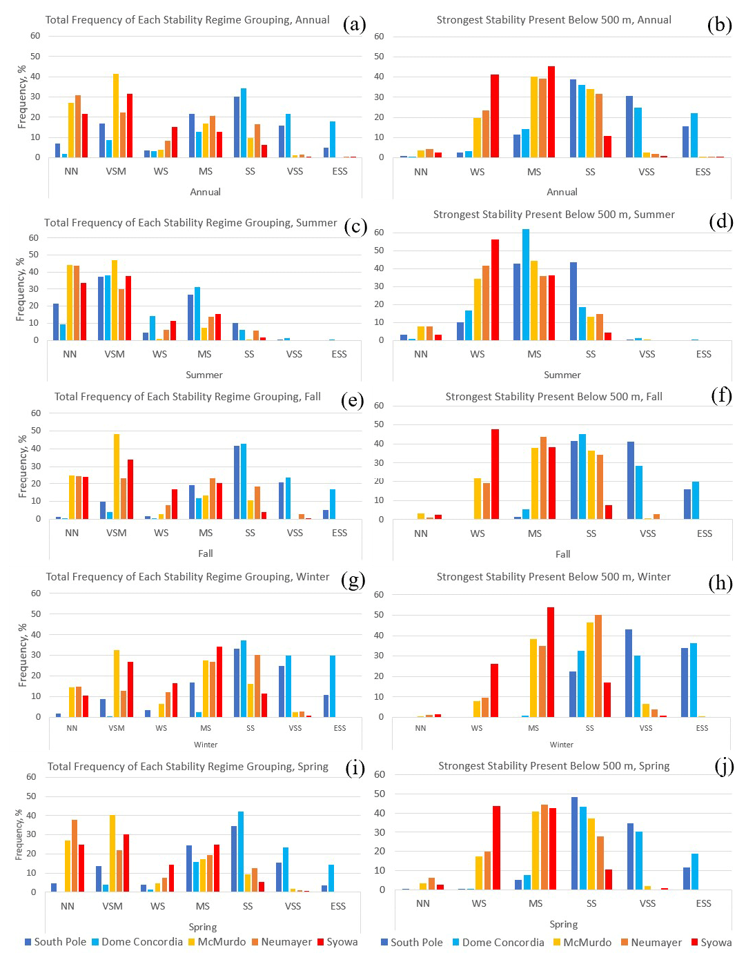
Figure 13Summary of the basic (a, c, e, g, i) near-surface stability regime frequency and (b, d, f, h, j) aloft stability regime frequency at all five sites (a, b) annually and (c–j) seasonally (summer, fall, winter, and spring). The colored bars indicate the frequency of each of the given regimes at each site: South Pole (dark blue), Dome C (light blue), McMurdo (yellow), Neumayer (orange), and Syowa (red).
It has been previously described in the literature that, even during austral summer, a temperature inversion is present nearly constantly (Hudson and Brandt, 2005; Genthon et al., 2013). Other studies, however, note the possibility of unstable conditions in the summer (King and Connolley, 1997; Mastrantonio et al., 1999; Pietroni et al., 2013). Thus, this study posed an opportunity to evaluate the range of stability present in the summer season across multiple Antarctic sites. Regimes with a near-surface stability of WS and weaker (Table S1) are the most common regimes at the interior sites in the summer (63.2 % of the time at South Pole and 61.4 % of the time at Dome C; Fig. 13c, Table S1). However, this weaker near-surface stability is often capped by stronger stability above the boundary layer such that when considering the maximum stability below 500 m, regimes with a stability of MS and stronger occur 86.7 % of the time at South Pole and 81.9 % of the time at Dome C. This indicates that moderate or stronger stability dominates aloft even though weaker stability occurs most of the time near the surface in the summer. This observation of enhanced stability above a weakly stable boundary layer has not been widely documented, much less quantified, especially in the continental interior of Antarctica. While winter at Dome C is characterized almost entirely by near-surface stability regimes of SS and stronger (96.9 %), the winter at South Pole experiences these regimes less often (68.8 %; Fig. 13g). However, when considering the maximum stability below 500 m (Fig. 13h), this reduced frequency of strong stability near the surface at South Pole compared to Dome C vanishes and regimes with a stability of SS and stronger occur nearly continuously and with a similar frequency at both South Pole and Dome C (99.6 % and 99.2 % of the time, respectively; Table S1).
Across all three coastal sites, a stability of WS and weaker near-surface occurs more than 50 % of the time in all seasons, except for Neumayer in the winter (Table S1). In the summer a near-surface stability of WS and weaker is dominant, occurring 80.1 % to 92.1 % of the time (Fig. 13c, Table S1). However, this high frequency of WS or weaker stability near the surface is not evident when stability aloft is considered and a stability of WS and weaker anywhere below 500 m occurs 42.1 % to 59.6 % of the time (Fig. 13d, Table S1). This indicates that while weaker near-surface stability is dominant in the summer at the coastal sites, a stability of MS or stronger is nearly as frequent as a stability of WS or weaker above the boundary layer. In the winter, a near-surface stability of WS and weaker occurs 40 % to 53.6 % of the time (Fig. 13g, Table S1), indicating a near even split between near-neutral to weak stability and moderate or stronger stability near the surface. In contrast, a stability of MS and stronger is observed within the lowest 500 m 72.1 % to 91.6 % of the time during the winter (Fig. 13h, Table S1), indicating that weak near-surface stability regimes usually have enhanced (MS or stronger) stability aloft. At McMurdo, the existence of enhanced stability above a layer of weaker stability was noted by Dice and Cassano (2022). Additionally, Silva et al. (2022) described the boundary layer at Neumayer ranging from strong surface-based temperature inversions to weak inversions near the surface with stronger inversions aloft throughout the year, which is also observed here. While both Dice and Cassano (2022) and Silva et al. (2022) noted the presence of enhanced stability above a layer of weaker stability, neither of these studies quantified the occurrence or seasonality of this phenomenon.
Comparing the coastal to the continental sites, near-surface stability regimes of WS and weaker are much more common at the coastal sites (61.3 % to 72.4 %) compared to the continental-interior sites (13.5 % to 27.2 %) on an annual basis (Table S1). When considering the maximum stability below 500 m, a stability of MS and stronger occurs nearly all of the time at the interior sites (96.5 % to 96.7 % of the time) and occurs more than half of the time at the coastal sites (56.5 % to 76.6 % of the time) annually (Table S1). This is consistent with observations from Zhang et al. (2011), who found that surface-based temperature inversions are less common along the coasts, as the coastal region is warmer, moister, and windier than the continental interior, which all reduces near-surface stability.
In the summer, a near-surface stability of WS or weaker occurs most of the time at all sites but is more frequent at the coastal (80.1 % to 92.1 % of the time) compared to the continental sites (61.4 % to 63.2 % of the time) (Table S1). In comparison, near-surface stability regimes of SS and stronger only occur 0.5 % to 5.9 % of the time at the coastal and 7.5 % to 10.3 % of the time at the interior sites, indicating the rarity of strong near-surface stability at both coastal and interior sites in the summer. However, when also considering stability just above the boundary layer, a stability of MS and stronger occurs more than 80 % of the time at both South Pole and Dome C (Table S1). Even at the coastal sites, a stability of MS and stronger occurs nearly half of the time (40.4 % to 57.9 %) in the summer (Table S1). These results highlight that while weak stability is usually present near the surface across the Antarctic continent in the summer, moderate or stronger stability is often present somewhere in the lowest 500 m of the atmosphere.
In the winter, strong stability is expected to be dominant across Antarctica (Lettau and Schwerdtfeger, 1967; Phillpot and Zillman, 1970; King and Turner, 1997; Andreas et al., 2000). Surprisingly, the near-surface stability of WS and weaker still occurs 40.0 % to 53.6 % of the time in the winter at the coastal sites, whereas these regimes, as expected, are infrequent at the interior sites, occurring 14.1 % of the time at South Pole and 0.8 % of the time at Dome C (Fig. 13g, Table S1). Near-surface stability stronger than SS occurs 12.3 % to 33.4 % of the time at the coastal sites and 68.8 % to 96.9 % of the time at the interior sites (Table S1), emphasizing the dominance of strong near-surface stability in the continental interior in the winter. When considering the maximum stability below 500 m, it is important to note that even though about half the time regimes of WS and weaker occur near the surface at the coastal sites, above the boundary layer enhanced stability remains. A stability of MS and stronger within the lowest 500 m of the atmosphere occurs 72.1 % to 91.6 % of the time at the coastal sites (Fig. 13h, Table S1). While there are very few cases with a near-surface stability of WS or weaker at the continental-interior sites in the winter, these always have enhanced stability above the boundary layer (Fig. 13h). The maximum stability below 500 m at the interior sites is almost always MS and stronger (99.8 % to 100 %), but, in fact, the maximum stability is almost just as often SS or stronger (99.2 % to 99.6 %) (Table S1). This emphasizes the near-complete dominance of the SS, VSS, and ESS regimes in the continental interior during the winter, while these regimes represent half or fewer (18.2 % to 54.3 %) of cases when considering maximum stability below 500 m at the coastal sites in the winter (Fig. 13h, Table S1).
It is also interesting to note the frequency of stability regimes in the spring and fall in comparison to that in the summer and winter at all five sites. At the interior sites, there is a tendency for the regime frequencies, whether considering just near-surface stability or the maximum stability in the lowest 500 m, in the fall and spring to mirror the winter season regime frequencies, and summer is completely distinct from the other seasons (Fig. 13c–j, Table S1). The most common near-surface stability groupings in the fall and spring are WS and weaker at the coastal sites (55.7 % to 71.8 % of the time; Fig. 13e and i), and these regimes are observed less frequently in the transition seasons than they are in the summer (80.1 % to 92.1 %; Fig. 13c) but more frequently than in the winter (40 % to 53.6 %; Fig. 13g). In comparison, the transition seasons at the continental-interior sites are usually characterized by MS and stronger stability near the surface (77.7 % to 95.4 %; Fig. 13f and j), which is similar to the frequency of these regimes in the winter as well (85.8 % to 99.5 %; Fig. 13g). Thus, at the interior sites, this comparison emphasizes the quick descent into the coreless winter from the transition seasons (Hudson and Brandt, 2005), whereas at the coastal sites, this change is more gradual.
To assess how applicable the commonly cited description of polar winter boundary layers of clear and strongly stable and cloudy and weakly stable (Stone and Kahl, 1991; Mahrt, 1998, 2014; Solomon et al., 2023) is for the Antarctic, we applied the method of Solomon et al. (2023) to identify clear and cloudy conditions, based on net longwave radiation. This approach for identifying clear and cloudy conditions was successful at the coastal Antarctic sites (Figs. S3 to S5) but was unable to identify distinct radiative signatures for clear or cloudy conditions at the two interior sites (Figs. S1 and S2). This suggests there may be fundamental differences in processes related to clouds, radiation, and stability on the polar plateau in comparison to the coastal region of Antarctica or over Arctic sea ice. Vignon et al. (2017) suggested that there may be two distinct boundary layer regimes (weakly stable and strongly stable) at Dome C, but, contrary to locations in the Arctic (Solomon et al., 2023), this is likely due to a critical shift in wind speeds, not a bimodal distribution in radiative forcing (Vignon et al., 2017).
For the three coastal sites, the frequency of the 20 boundary layer stability regimes defined in Table 2 was calculated for clear and cloudy conditions (Fig. 12). This analysis revealed regimes of MS and stronger occur more often with clear conditions rather than cloudy conditions at McMurdo and Neumayer. The NN and WS regime grouping at McMurdo (excluding NN-SSA) and the NN regime grouping at Neumayer occur more often with cloudy rather than clear conditions, but these are the only stability regimes in this analysis in which there is a large difference in frequency for cloudy or clear conditions. At Syowa, there is little difference in the frequency of any stability regime for both clear and cloudy conditions. The fact that some stability regimes at McMurdo and Neumayer and all the stability regimes at Syowa show little sensitivity to changes in cloud cover suggests a more nuanced relationship between radiative forcing and near-surface stability may exist in the Antarctic compared to the Arctic, and other forcing mechanisms, such as mechanical mixing, may be relatively more important in distinguishing boundary layer stability regimes from one another. Mahrt (2014) noted that weakly stable conditions occur with either cloud cover or increased wind and mentioned that classification into the weakly stable and strongly stable regimes does not encompass the full complexity of forcing in the stable boundary layer.
A useful next step in this research will be to more thoroughly assess the forcing for the different stability regimes. Largely, radiative forcing and mechanical mixing (wind shear) are two main drivers of boundary layer stability. The role of these two processes, not only across seasons at the individual sites but also across the five sites, will be the basis of continued research. Assessing forcing for regimes that showed little sensitivity to cloud cover is of interest since it appears that changes in radiative forcing may not play a dominant role. A paper following this study will use the boundary layer regimes identified for each individual radiosonde profile to identify variations in radiation and wind speed associated with the different stability regimes. Further, an analysis of the ability of the Antarctic Mesoscale Prediction System (AMPS; Powers et al., 2012) to simulate the range of stability regimes observed at each site and the radiative and mechanical forcing associated with these regimes across Antarctica is planned.
The data used to support this project can be found at the following resources.
For McMurdo, all data can be found at https://adc.arm.gov/discovery/#/results/site_code::awr (ARM, 2023).
For Syowa, radiosonde data can be found at the Office of Antarctic Observation of the Japan Meteorological Agency (Yutaka Ogawa, personal communication, 2021) and radiation data can be found at https://doi.pangaea.de/10.1594/PANGAEA.956748 (Ogawa et al., 2023).
For Dome C, radiosonde data can be found at https://www.climantartide.it/dataaccess/rds/index.php?lang=it&rds=DOMEC (RDS Concordia, 2023) and radiation data can be found at https://doi.org/10.1594/PANGAEA.935421 (Lupi et al., 2021).
For South Pole, radiosonde data can be found at http://amrc.ssec.wisc.edu/data/ftp/pub/southpole/radiosonde/ (AMRC, 2023) and radiation data can be found at https://doi.org/10.1594/PANGAEA.956847 (Riihimaki et al., 2023).
For Neumayer, radiosonde data can be found at https://doi.org/10.1594/PANGAEA.940584 (Schmithüsen, 2022).
The supplement related to this article is available online at: https://doi.org/10.5194/wcd-4-1045-2023-supplement.
JJC acquired funding for analysis; MS provided software guidance and code; MD, GCJ, and JJC conceptualized the analysis presented in this paper; MD analyzed the data; MD wrote the manuscript; and JJC, MD, MS, and GCJ reviewed and edited the manuscript.
The contact author has declared that none of the authors has any competing interests.
Publisher's note: Copernicus Publications remains neutral with regard to jurisdictional claims made in the text, published maps, institutional affiliations, or any other geographical representation in this paper. While Copernicus Publications makes every effort to include appropriate place names, the final responsibility lies with the authors.
The authors thank the United States Antarctic Program, the Department of Energy, the Baseline Surface Radiation Network, the Antarctic Meteorological Research and Data Center, the Antarctic Meteo-Climatological Observatory, and the Office of Antarctic Observation of the Japan Meteorological Agency for the support and logistics for the data used in this paper.
This research has been supported by the National Science Foundation (grant no. OPP 1745097) and the National Aeronautics and Space Administration (grant no. 80NSSC19M0194).
This paper was edited by Tiina Nygård and reviewed by John King and one anonymous referee.
AMRC: Index of /data/ftp/pub/southpole/radiosonde, AMRC [data set], http://amrc.ssec.wisc.edu/data/ftp/pub/southpole/radiosonde/ (last access: 29 November 2023), 2023.
Andreas, E. L., Claffy, K. J., and Makshtas, A. P.: Low-level atmospheric jets and inversions over the western Weddell Sea, Bound.-Lay. Meteorol., 97, 459–486, https://doi.org/10.1023/A:1002793831076, 2000.
Aristidi, E., Agabi, K., Azouit, M., Fossat, E., Vernin, J., Travouillon, T., Lawrence, J. S., Meyer, C., Storey, J. W. V., Halter, B., Roth, W. L., and Walden, V.: An analysis of temperatures and wind speeds above Dome C, Antarctica, Astron. Astrophys., 430, 739–746, https://doi.org/10.1051/0004-6361:20041876, 2005.
ARM: https://adc.arm.gov/discovery/#/results/site_code::awr, last access: 29 November 2023.
Cassano, E. N., Glisan, J. M., Cassano, J. J., Gutowski Jr., W. J., and Seefeldt, M. W.: Self-organizing map analysis of widespread temperature extremes in Alaska and Canada, Clim. Res., 62, 199–218, https://doi.org/10.3354/cr01274, 2015.
Cassano, J. J., Nigro, M., and Lazzara, M.: Characteristics of the near surface atmosphere over the Ross ice shelf, Antarctica, J. Geophys. Res.-Atmos., 121, 3339–3362, https://doi.org/10.1002/2015JD024383, 2016.
Chechin, D. G., Lüpkes, C., Hartmann, J., Ehrlich, A., and Wendisch, M.: Turbulent structure of the Arctic boundary layer in early summer driven by stability, wind shear and cloud-top radiative cooling: ACLOUD airborne observations, Atmos. Chem. Phys., 23, 4685–4707, https://doi.org/10.5194/acp-23-4685-2023, 2023.
Comiso, J. C.: Surface temperatures in the polar regions from Nimbus 7 temperature humidity infrared radiometer, J. Geophys. Res., 99, 5181–5200, https://doi.org/10.1029/93JC03450, 1994.
Connolley, W. M.: The Antarctic temperature inversion, Int. J. Climatol., 16, 1333–1342, 1996.
Dice, M. J. and Cassano, J. J.: Assessing physical relationships between atmospheric state, fluxes, and boundary layer stability at McMurdo Station, Antarctica, J. Geophys. Res.-Atmos., 127, e2021JD036075, https://doi.org/10.1029/2021JD036075, 2022.
Ganeshan, M., Yang, Y., and Palm, S. P.: Impact of clouds and blowing snow on surface and atmospheric boundary layer properties over Dome C, Antarctica, J. Geophys. Res.-Atmos., 127, e2022JD036801, https://doi.org/10.1029/2022JD036801, 2022.
Genthon, C., Six, D., Gallée, H., Grigioni, P., and Pellegrini, A.: Two years of atmospheric boundary layer observations on a 45-m tower at Dome C on the Antarctic plateau, J. Geophys. Res.-Atmos., 118, 3218–3232, https://doi.org/10.1002/jgrd.50128, 2013.
Handorf, D., Foken, T., and Kottmeier, C.: The stable atmospheric boundary layer over an Antarctic ice sheet, Bound.-Lay. Meteorol., 91, 165–189, https://doi.org/10.1023/A:1001889423449, 1999.
Hewitson, B. C. and Crane, R. G.: Self-organizing maps: Applications to synoptic climatology, Clim. Res., 22, 13–26, https://doi.org/10.3354/cr022013, 2002.
Hudson, S. and Brandt, R.: A look at the surface-based temperature inversion on the Antarctic Plateau, J. Climate, 18, 1673–1696, https://doi.org/10.1175/JCLI3360.1, 2005.
Jozef, G., Cassano, J., Dahlke, S., and de Boer, G.: Testing the efficacy of atmospheric boundary layer height detection algorithms using uncrewed aircraft system data from MOSAiC, Atmos. Meas. Tech., 15, 4001–4022, https://doi.org/10.5194/amt-15-4001-2022, 2022.
Jozef, G. C., Cassano, J. J., Dahlke, S., Dice, M., Cox, C. J., and de Boer, G.: An Overview of the Vertical Structure of the Atmospheric Boundary Layer in the Central Arctic during MOSAiC, EGUsphere [preprint], https://doi.org/10.5194/egusphere-2023-780, 2023.
King, J. C. and Connolley, W. M.: Validation of the Surface Energy Balance over the Antarctic Ice Sheets in the U.K. Meteorological Office Unified Climate Model, J. Climate, 10, 1273–1287, https://doi.org/10.1175/1520-0442(1997)010<1273:VOTSEB>2.0.CO;2, 1997.
King, J. C. and Turner, J.: Antarctic Meteorology and Climatology, Cambridge Atmospheric and Space Sciences Series, Cambridge University Press, UK, https://doi.org/10.1017/CBO9780511524967, 1997.
Kohonen, T., Hynninen, J., Kangas, J., and Laaksonen, J.: SOMPAK: The Self-Organizing Map Program Package, Rep. A31, Lab. Of Comput. and Inf. Sci., Helsinki Univ. of Technol., Espoo, Finland, https://www.researchgate.net/publication/2596686_SOM_PAK_The_self-organizing_map_program_package (last access: 29 November 2023), 1996.
König-Langlo, G. and Loose, B.: The Meteorological Observatory at Neumayer Stations (GvN and NM-II) Antarctica, Polarforschung, 76, 25–38, 2007.
Lettau, H. H. and Schwerdtfeger, W.: Dynamics of the Surface-Wind RegimeOver the Interior of Antarctica, Antarct. J., 2, 155–158, 1967.
Lubin, D., Bromwich, D. H., Vogelmann, A. M., Verlinde, J., and Russell, L. M.: ARM West Antarctic Radiation Experiment (AWARE) Field Campaign Report, DOE/SC-ARM-17-028, https://www.arm.gov/publications/programdocs/doe-sc-arm-17-028.pdf (last access: 29 November 2023), 2017.
Lubin, D., Zhang, D., Silber, I., Scott, R. C., Kalogeras, P., Battaglia, A., Bromwich, D. H., Cadeddu, M., Eloranta, E., Fridlind, A., Frossard, A., Hines, K., Kneifel, S., Leaitch, W. R., Lin, W., Nicolas, J., Powers, H., Quinn, P. K., Rowe, P., Russell, L. M., Sharma, S., Verlinde, J., and Vogelmann, A. M.: AWARE: The atmospheric radiation measurement (ARM) West Antarctic radiation experiment, B. Am. Meteorol. Soc., 101, E1069–E1091, https://doi.org/10.1175/BAMS-D-18-0278.1s, 2020.
Lupi, A., Lanconelli, C., and Vitale, V.: Basic and other measurements of radiation at Concordia station (2006-01 et seq). Institute of Atmospheric Sciences and Climate of the Italian National Research Council, Bologna, PANGAEA [data set], https://doi.org/10.1594/PANGAEA.935421, 2021.
Mahesh, A., Walden, V. P., and Warren, S. G.: Radiosonde Temperature Measurements in Strong Inversions: Correction for Thermal Lag Based on an Experiment at the South Pole, J. Atmos. Ocean. Tech., 14, 45–53, https://doi.org/10.1175/1520-0426(1997)014<0045:RTMISI>2.0.CO;2, 1997.
Mahrt, L.: Stratified atmospheric boundary layers and breakdown of models, Theor. Comput. Fluid Dynam., 11, 263–280, 1998.
Mahrt, L.: Stably Stratified Atmospheric Boundary Layers, Annu. Rev. Fluid Mech., 46, 23–45, https://doi.org/10.1146/annurev-fluid-010313-141354, 2014.
Mastrantonio, G., Malvestuto, V., Argentini, S., Georgiadis, T., and Viola, A.: Evidence of a convective boundary layer developing on the Antarctic Plateau during the summer, Meteorol. Atmos. Phys., 71, 127–132, https://doi.org/10.1007/s007030050050, 1999.
Matsuoka, K., Skoglund, A., and Roth, G.: Quantarctica, Norwegian Polar Institute [data set], https://doi.org/10.21334/npolar.2018.8516e961, 2018.
Morley, B. M., Uthe, E. E., and Viezee, W.: Airborne lidar observations of clouds in the Antarctic troposphere, Geophys. Res. Lett., 16, 491–494, https://doi.org/10.1029/GL016i006p00491, 1989.
Murakoshi, N.: Meteorological observations at the Syowa base during the period from March 1957 to February 1958, Japan Meteorological Agency, https://doi.org/10.15094/00006856, 1958.
Nigro, M. A., Cassano, J. J., Wille, J., Bromwich, D. H., and Lazzara, M. A.: A Self-Organizing-Map-Based Evaluation of the Antarctic Mesoscale Prediction System Using Observations from a 30-m Instrumented Tower on the Ross Ice Shelf, Antarctica, Weather Forecast., 32, 223–242, https://doi.org/10.1175/WAF-D-16-0084.1, 2017.
Ogawa, Y., Tanaka, Y., Ogihara, H., Fukuda, M., Kawashima, K., Doi, M., and Yamanouchi, T.: Basic and other measurements of radiation at station Syowa (1994-01 et seq). National Institute of Polar Research, Tokyo, PANGAEA [data set], https://doi.pangaea.de/10.1594/PANGAEA.956748, 2023.
Phillpot, H. R., and Zillman, J. W.: The surface temperature inversion over the Antarctic continent, J. Geophys. Res., 75, 4161–4169, https://doi.org/10.1029/JC075i021p04161, 1970.
Pietroni, I., Argentini, S., Petenko, I., and Sozzi, R.: Measurements and Parametrizations of the Atmospheric Boundary-Layer Height at Dome C, Antarctica, Bound.-Lay. Meteorol., 143, 189–206, https://doi.org/10.1007/s10546-011-9675-4, 2012.
Pietroni, I., Argentini, S., and Petenko, I.: One Year of Surface-Based Temperature Inversions at Dome C, Antarctica, Bound.-Lay. Meteorol., 150, 131–151, 2013.
Powers, J. G., Manning, K. W., Bromwich, D. H., Cassano, J. J., and Cayette, A. M.: A Decade of Antarctic Science Support Through AMPS, B. Am. Meteorol. Soc., 93, 1699–1712, https://doi.org/10.1175/BAMS-D-11-00186.1, 2012.
RDS Concordia: Osservatorio Meteo-Climatologico Antartico, https://www.climantartide.it/dataaccess/rds/index.php?lang=it&rds=DOMEC (last access: 29 November 2023), 2023.
Reusch, D. B., Alley, R. B., and Hewitson, B. C.: Relative performance of self-organizing maps and principal component analysis in pattern extraction from synthetic climatological data, Polar Geogr., 29, 188–212, https://doi.org/10.1080/789610199, 2005.
Riihimaki, L., Long, C. E., Dutton, E. G., and Michalsky, J.: Basic and other measurements of radiation at station South Pole (1992-01 et seq). NOAA Global Monitoring Laboratory, Boulder, PANGAEA [data set], https://doi.org/10.1594/PANGAEA.956847, 2023.
Schmithüsen, H.: Radiosonde measurements from Neumayer Station (1983-02 et seq). Alfred Wegener Institute, Helmholtz Centre for Polar and Marine Research, Bremerhaven, PANGAEA [data set], https://doi.org/10.1594/PANGAEA.940584, 2022.
Schwartz, B. E., and Doswell III, C. A.: North American Rawinsonde Observations: Problems, Concerns, and a Call to Action, B. Am. Meteorol. Soc., 72, 1885–1896, https://doi.org/10.1175/1520-0477(1991)072<1885:NAROPC>2.0.CO;2, 1991.
Silber, I., Verlinde, J., Eloranta, E. W., and Cadeddu, M.: Antarctic Cloud macrophysical, thermodynamic phase, and atmospheric inversion coupling properties at McMurdo station: I. Principal data processing and climatology, J. Geophys Res.-Atmos., 123, 6099–6121, https://doi.org/10.1029/2018JD028279, 2018.
Silva, T., Schlosser, E., and Lehner, M.: A 25-year climatology of low-tropospheric temperature and humidity inversions for contrasting synoptic regimes at Neumayer Station, Antarctica, Int. J. Climatol., 43, 456–479, https://doi.org/10.1002/joc.7780, 2022.
Solomon, A., Shupe, M. D., Svensson, G., Barton, N. P., Batrak, Y., Bazile, E., Day, J. J., Doyle, J. D., Frank, H. P., Keeley, S., Remes, T., and Tolstykh, M.: The winter central Arctic surface energy budget: A model evaluation using observations from the MOSAiC campaign, Elementa, 11, 00104, https://doi.org/10.1525/elementa.2022.00104, 2023.
Stone, R. S. and Kahl, J. D.: Variations in boundary layer properties associated with clouds and transient weather disturbances at the South Pole during winter, J. Geophys. Res., 96, 5137–5144, https://doi.org/10.1029/90JD02605, 1991.
Stull, R. B.: An Introduction to Boundary Layer Meteorology, Springer, ISBN 902772768-6, 1988.
Town, M. S., Walden, V. P., and Warren, S. G.: Spectral and Broadband Longwave Downwelling Radiative Fluxes, Cloud Radiative Forcing, and Fractional Cloud Cover over the South Pole, J. Climate, 18, 4235–4252, https://doi.org/10.1175/JCLI3525.1, 2005.
Town, M. S., Walden, V. P., and Warren, S. G.: Cloud Cover over the South Pole from Visual Observations, Satellite Retrievals, and Surface-Based Infrared Radiation Measurements, J. Climate, 20, 544–559, https://doi.org/10.1175/JCLI4005.1, 2007.
Vignon, E., van de Wiel, B. J. H., van Hooijdonk, I. G. S., Genthon, C., van der Linden, S. J. A., van Hooft, J. A., Baas, P., Maurel, W., Traulle, O., and Casasanta, G.: Stable boundary-layer regimes at Dome C, Antarctica: observation and analysis, Q. J. Roy. Meteorol. Soc., 143, 1241–1253, https://doi.org/10.1002/qj.2998, 2017.
Yamada, K. and Hirasawa, N.: of a Record-Breaking Strong Wind Event at Syowa Station in January 2015, J. Geophys. Res.-Atmos., 123, 13643–13657, https://doi.org/10.1029/2018JD028877, 2018.
Zhang, Y., Seidel, D., Golaz, J., Deser, C., and Tomas, R.: Climatological characteristics of Arctic and Antarctic surface-based inversions, J. Climate, 24, 5167–5186, https://doi.org/10.1175/2011JCLI4004.1, 2011.