the Creative Commons Attribution 4.0 License.
the Creative Commons Attribution 4.0 License.
 | 31 Jul 2023
On the linkage between future Arctic sea ice retreat, Euro-Atlantic circulation regimes and temperature extremes over Europe
Johannes Riebold
Andy Richling
Uwe Ulbrich
Henning Rust
Tido Semmler
Dörthe Handorf
The question to what extent Arctic sea ice loss is able to affect atmospheric dynamics and climate extremes over mid-latitudes still remains a highly debated topic. In this study we investigate model experiments from the Polar Amplification Model Intercomparison Project (PAMIP) and compare experiments with future sea ice loss prescribed over the entire Arctic, as well as only locally over the Barents and Kara seas, with a present-day reference experiment. The first step is to perform a regime analysis and analyze the change in occurrence frequencies of five computed Euro-Atlantic winter circulation regimes. Forced by future Arctic sea ice conditions, most models show more frequent occurrences of a Scandinavian blocking pattern in at least 1 winter month, whereas there is an overall disagreement between individual models on the sign of frequency changes of two regimes that, respectively, resemble the negative and positive phase of the North Atlantic Oscillation. Focusing on the ECHAM6 PAMIP experiments, we subsequently employ a framework of conditional extreme-event attribution. It demonstrates how detected regime frequency changes can be used to decompose sea-ice-induced frequency changes of European temperature extremes into two different contributions: one “changed-regime” term that is related to dynamical changes in regime occurrence frequencies and another more thermodynamically motivated “fixed-regime” contribution that is related to increased surface temperatures during a specific circulation regime. We show how the overall fixed-regime warming effect and also an increased Scandinavian blocking pattern frequency under future sea ice reductions can equally contribute to and shape the overall response signal of European cold extremes in midwinter. We also demonstrate how a decreased occurrence frequency of an anticyclonic regime over the eastern Atlantic dynamically counteracts the fixed-regime warming response and results in no significant changes in overall January warm-extreme occurrences. However, when compared to other characteristics of future climate change, such as the thermodynamical impact of globally increased sea surface temperatures, the effects of Arctic sea ice loss on European temperature extremes are of secondary relevance.
- Article
(9381 KB) - Full-text XML
-
Supplement
(5635 KB) - BibTeX
- EndNote


Recent global warming includes a phenomenon called Arctic amplification that entails an up to 4 times faster warming of Arctic regions compared to global average over recent decades (Rantanen et al., 2022). This amplified Arctic warming is predominantly observed in wintertime and is accompanied by an unprecedented shrinkage of Arctic sea ice concentration and thickness (Stroeve and Notz, 2018). Model projections forced under different greenhouse gas scenarios show clear evidence of a continuation of sea ice decline, with some models suggesting a seasonally ice-free Arctic by the middle of the century (Notz and SIMIP Community, 2020). Aside from local ecological and economical impacts (Meredith et al., 2019), the question to what extent Arctic climate change and related sea ice loss may impact mid-latitude weather and general atmospheric dynamics has received a lot of attention over the last few years and decades (e.g., Cohen et al., 2020; Screen, 2017b; Handorf et al., 2015; Cohen et al., 2014). A large variety of potential hemispheric-wide atmospheric responses have been detected and hypothesized in connection to Arctic sea ice loss. Such responses include for instance a commonly observed negative winter North Atlantic Oscillation (NAO) response (e.g., Screen, 2017b; Nakamura et al., 2015; Jaiser et al., 2012), a highly debated weakening and stronger meandering of the jet stream that may result in more stationary and more slowly propagating large-scale Rossby waves (Francis and Vavrus, 2012; Barnes and Screen, 2015; Riboldi et al., 2020), and an intensification of the Scandinavian and Ural highs leading to continental winter cooling over Eurasia (Cohen et al., 2018). In this respect, dynamical pathways have been proposed relating for instance sea ice and snow cover anomalies in autumn to enhanced vertical wave activity fluxes and a weakened stratospheric polar vortex (Smith et al., 2022). These stratospheric disturbances could subsequently propagate downwards and finally result in a late winter negative NAO response (Cohen et al., 2014; Nakamura et al., 2016; Jaiser et al., 2016; Sun et al., 2015). Especially the Barents–Kara sea region, being a hotspot of recent Arctic sea ice retreat, has been argued to play an essential role in triggering such dynamical pathways (Screen, 2017a; Jaiser et al., 2016; Kretschmer et al., 2016). Nevertheless, no overall consensus about linkages and the underlying dynamical pathways has been reached yet (Cohen et al., 2020; Blackport and Screen, 2020), mostly due to discrepancies between observational and modeling studies. A recent study by Siew et al. (2020) highlighted for instance that the intermittent and state-dependent character of the aforementioned stratospheric pathway might be a potential reason for the typical low signal-to-noise ratios of atmospheric responses to sea ice changes. Furthermore, Petoukhov and Semenov (2010) showed how the modeled atmospheric response can depend on the magnitude of prescribed sea ice loss in the Barents and Kara seas in a highly nonlinear way. Although most studies on Arctic–mid-latitude linkages focus on the role of sea ice changes, several recent studies (He et al., 2020; Labe et al., 2020) have also highlighted the importance of the vertical extent of Arctic warming into the upper troposphere compared to sea ice loss alone.
From a more large-scale and regime-oriented perspective, atmospheric dynamics can be viewed in a variety of conceptual frameworks (Hoskins and Woollings, 2015), including for instance jet stream states, blocking or atmospheric circulation regimes. Especially the framework of circulation regimes has been employed in a large variety of studies (e.g., Crasemann et al., 2017; Horton et al., 2015) in order to characterize atmospheric circulation. Circulation regimes provide physically meaningful categorizations (Hochman et al., 2021) of atmospheric low-frequency variability into different regime states and have also been associated with preferred or quasi-stationary states of the underlying nonlinear atmospheric system (Hannachi et al., 2017). It has been hypothesized that weak external forcings imposed onto the atmospheric system are able to modify the occurrence probability of such regime states (Corti et al., 1999; Gervais et al., 2016) while not affecting the overall regime structure (Palmer, 1999). Indeed, Crasemann et al. (2017) compared atmosphere-only model experiments forced under conditions of low and high sea ice relative to the recent past and showed how the occurrence probability of certain Euro-Atlantic circulation regimes can be significantly affected by such Arctic sea ice changes. In this case the induced sea ice changes were considered weak forcings applied to the atmospheric system.
Of major interest for human society nowadays is the question to what extent the recently observed increasing number of climate extremes (Coumou and Rahmstorf, 2012) can be attributed to and are affected by anthropogenic global warming (Otto, 2016). Basically, there is an overall agreement that from a thermodynamical perspective, global warming will lead to less (more) frequent and intense cold (warm) extremes. Nevertheless, the occurrence of cold spells like that over Europe in 2010 (Cattiaux et al., 2010) or the more recent cold-air outbreak over North America in 2021 (Bolinger et al., 2022) might be considered contradictions to this simplified thermodynamical perspective.
In this respect, Cattiaux et al. (2010) illustrated for instance how the European winter cold spell in 2010 was, from a thermodynamical point of view, perfectly in line with recent global warming when accounting for the anomalous negative NAO situation during that winter. Shepherd (2016) framed a storyline approach aiming to separate specific classes of extreme events into different contributing factors by including both dynamical and non-dynamical contributions. However, circulation changes found in climate model simulations typically suffer low signal-to-noise ratios (Scaife and Smith, 2018; Smith et al., 2022). Therefore, changes regarding the dynamical situation leading to a certain extreme should only be included in an analysis when there is solid evidence that changes in atmospheric circulation can be expected or reliably detected (Trenberth et al., 2015; Shepherd, 2016).
Since, as mentioned above, Arctic sea ice retreat has been proven to be potentially able to modify atmospheric large-scale dynamics, the question appeared how changes in mid-latitude weather can be dynamically and thermodynamically attributed to Arctic sea ice changes. Screen (2017b) compared large ensembles of atmosphere-only experiments forced under conditions of low and high sea ice relative to the recent past. They observed that despite an intensification of negative winter NAO events under conditions of low Arctic sea ice, an expected dynamically induced European cooling response was absent, mostly due to compensation effects related to an overall thermodynamical warming. Another study by Deser et al. (2016a) investigated how different complexities of an ocean model can affect the large-scale hemispheric circulation response to Arctic sea ice loss. They compared model simulations with Arctic sea ice conditions constrained to the late 21st and 20th century. On the one hand they argued that under reduced-sea-ice conditions elevated sea level pressures over northern Siberia and Arctic regions are associated with anomalous northeasterly advection of cold Arctic air masses towards central Eurasia. This dynamically induces a cooling response over the respective central Eurasian regions. On the other hand, this dynamical cooling effect may be thermodynamically counteracted by elevated sea surface temperatures (SSTs), which was especially the case for coupled ocean–atmosphere model setups. Recent studies however argue that such coupled model setups artificially overestimate the impact of sea ice loss (England et al., 2022). Recently, Chripko et al. (2021) studied fully coupled model experiments where the sea ice albedo parameter was reduced to an ocean value yielding mostly ice-free conditions from July to October and moderate sea ice reductions in winter. When compared to a control simulation they detected winter warming signals over Europe and North America in the sensitivity experiment. By applying a dynamical adjustment method (Deser et al., 2016b), they showed that these overall responses could be explained by a combination of a dynamical response and a residual contribution.
Based on such previous studies that decomposed changes in mid-latitude weather and dynamics and linked them to Arctic sea ice loss, as well as due to the high societal relevance of extreme events nowadays, the question arises to what extent future sea ice retreat is able to impact the occurrence of extreme weather events.
Therefore, in this study we investigate the impact of future Arctic sea ice loss on the mid-latitude circulation over the Euro-Atlantic domain and related European temperature extremes. Here, we will focus on winter temperature extremes over the European region that can have significant impacts on society (Díaz et al., 2005) and the economy (Savić et al., 2014; Añel et al., 2017) over such densely populated regions. In order to assess and isolate the impact of Arctic sea ice changes, we will investigate model experiments from the Polar Amplification Model Intercomparison Project (PAMIP). The experiments that are considered here are forced under present-day conditions and future conditions of reduced sea ice over the entire Arctic, as well as under sea ice conditions only locally reduced over the Barents and Kara seas. The latter allows for assessing the role of sea ice loss specifically in the Barents and Kara sea region. Focusing on circulation changes detected in the ECHAM6 model, as well as employing a framework of conditional extreme-event attribution (Yiou et al., 2017), we will demonstrate how overall sea-ice-induced changes in extreme occurrences can be decomposed into two different contributions: first, one fixed-regime term that compares extreme occurrence frequencies for a given and fixed circulation regime and, secondly, a changed-regime contribution term that is related to changes in occurrence frequencies of the respective regime. More specifically, the analysis steps can be divided into different research questions that are partially linked to each other:
-
Within the methodological framework of atmospheric circulation regimes, what changes in the wintertime atmospheric large-scale circulation over the Euro-Atlantic sector can be expected under future Arctic sea ice retreat?
-
Which regimes can be associated with preferred occurrences of winter temperature extremes over Europe?
-
What overall frequency changes of extreme occurrences over the continental Northern Hemisphere can be detected in response to future sea ice changes in ECHAM6?
-
Based on the sea-ice-induced changes in circulation regimes detected in ECHAM6, to what extent can frequency changes of European extremes be related to fixed-regime and changed-regime contributions?
When studying the impact of Arctic sea ice changes on mid-latitude circulation and weather, the question may arise how such impacts compare to atmospheric responses induced by other facets of future climate change. Therefore, in order to assess the relative importance of sea ice loss to future changes in European extremes, the analysis will be complemented by investigating the impact of a globally increased future SST background state prescribed in one of the experimental setups.
In this study we initially analyze different sea ice sensitivity simulation data from the Polar Amplification Model Intercomparison Project (PAMIP; Smith et al., 2019). Table S1 in the Supplement provides an overview of the models and ensemble sizes considered. The PAMIP protocol aims at a better understanding of the impact of Arctic sea ice and SST changes on the global climate system and their relative roles in this system. Therefore, each sensitivity experiment includes at least 100 ensemble members of 1-year-long atmosphere-only time slice simulations that are forced under different annual cycles of sea ice and also SST boundary conditions. As recommended by Smith et al. (2019), initial conditions of each ensemble member are based on conditions for 1 April 2000 from the Atmospheric Model Intercomparison Project (AMIP) simulations for 1 April 2000 and each ensemble member was run for 14 months, but the first 2 months was ultimately excluded for model spin-up reasons. In order to study the impact of future sea ice changes on circulation regimes, we analyze sensitivity simulations forced under
-
present-day SST and present-day sea ice conditions (pdSIC, PAMIP setup 1.1)
-
present-day SST and future/reduced Arctic-wide sea ice conditions (futArcSIC, PAMIP setup 1.6)
-
present-day SST and future/reduced sea ice in the Barents and Kara sea region, 65–85∘ N, 10–110∘ E (futBKSIC, PAMIP setup 3.2).
For the analyses in Sect. 4.2–4.4, we focus on the 100 ensemble members from the ECHAM6 experiments. ECHAM6 is the latest release of the atmospheric general circulation model ECHAM that was developed at the Max Planck Institute for Meteorology (MPI) in Hamburg (Stevens et al., 2013). The ECHAM6 setup used for the PAMIP experiments operates on 95 vertical layers up to 0.01 hPa and with a spectral T127 horizontal resolution (resulting in a zonal resolution of 100 km in the tropics and for instance 25 km at 75∘ N). In order to contrast the importance of future SST with Arctic sea ice changes at the very end of this study, we also consider 100 ensemble members from an ECHAM6 sensitivity simulation forced under
-
present-day sea ice and globally raised future SST conditions (futSST, PAMIP setup 1.4).
The pdSIC simulations serve in the first place as reference simulations to which the sensitivity simulations futArcSIC and futBKSIC are compared. Comparisons of sea ice and SST forcing fields of the respective present-day and sea ice sensitivity simulations are shown in Smith et al. (2019) in Figs. 5 and 6. In winter, future sea ice conditions are predominantly reduced over the Barents and Kara seas, the Sea of Okhotsk, the Bering Sea, and parts west and east of Greenland. Summer conditions are characterized by strong reductions and ice-free areas over central Arctic regions.
Present-day forcing fields are obtained from the climatologies of observations from the Hadley Centre Sea Ice and Sea Surface Temperature dataset over the period 1979–2008 (Rayner et al., 2003). Future conditions are derived from Representative Concentration Pathway 8.5 (RCP8.5) multimodel simulations for a 1.43 (2) ∘C warming scenario under present-day (preindustrial) conditions (for more details see Smith et al., 2019, their Appendix A). At grid points where sea ice has been removed under future conditions, the present-day SSTs are replaced by future SSTs if the difference in sea ice concentration between the future and the present day is greater than 10 %. Sea ice thickness at each grid point is set to 2 m for all simulations, and greenhouse gas forcings are constantly set to present-day conditions of the year 2000.
For the analysis presented in this study, we use daily sea level pressure (slp) data from all PAMIP models, as well as daily maximum and minimum near-surface air temperatures (Tmax and Tmin) from ECHAM6. The daily temperature and slp data in ECHAM6 are provided on a regular longitude–latitude grid with 0.9375∘ resolution. The slp data from ECHAM6 (and from all other PAMIP models as well) are however finally regridded to a 100 km × 100 km equal-area grid (see also next section).
In order to complement and back up certain parts of our analysis with real-world data, we additionally used slp, 2 m temperature and sea ice area data from the ERA5 reanalysis over the period 1979–2018 (Hersbach et al., 2020).
3.1 Circulation regimes
In this study, we compute centroids Ci of atmospheric circulation regimes for the extended winter season with the k-means clustering algorithm (Michelangeli et al., 1995; Crasemann et al., 2017; Straus et al., 2007) applied to daily slp anomaly data merged together from two different experiments (typically the pdSIC reference simulation and one of the sensitivity simulations) over the Euro-Atlantic domain (20 to 88∘ N, −90 to 90∘ W). Before applying the clustering algorithm, slp data were regridded to a 100 km × 100 km equal-area grid in order to avoid grid point convergence at higher latitudes. Generally speaking k-means clustering aims to minimize the variance ratio of the intra-cluster to inter-cluster by an iterative allocation and exchange procedure of cluster members (MacQueen, 1967). In order to reduce computational demands, we applied a dimensionality reduction via principal component analysis prior to the clustering algorithm. Here we used the first 20 principal components that roughly explain around 90 % of variance of the winter slp anomaly fields. Further increasing the number of principal components did not affect the final outcome of the clustering algorithm. The k-means algorithm has been initialized 1000 times, and the best result in terms of minimizing the aforementioned variance ratio has been finally chosen. Based on the Euclidean distance, the respective slp anomaly field or atmospheric flow F on each day is finally assigned to the best-matching cluster centroid Ci.
Anomalies of slp are generally calculated as deviations from an annual cycle, which is obtained by averaging each day of a year over all years. For the merged pdSIC+futBKSIC and pdSIC+futArcSIC datasets, we computed a joint annual cycle of both simulations. It shows that the resulting cluster allocations are not considerably affected by whether the slp anomalies have been calculated either as deviations from the joint annual cycle as described above or by removing the annual cycles for each experiment individually (as done by, e.g., Crasemann et al., 2017). This is also related to the fact that when contrasting the reference with both sea ice sensitivity experiments, the respective winter slp background states showed mostly negligible differences, nor did they project onto any mode of variability. In contrast to the sea ice sensitivity simulations, the relatively strong forcing in the ECHAM6 futSST experiment leads to an evident change in the slp background state (with respect to the reference simulation) that strongly projects onto a positive NAO pattern. This background difference pattern significantly affects the final cluster allocations when subtracting a joint annual cycle. Therefore, we computed the annual cycle for both simulations individually when merging data from the futSST and the pdSIC experiments to take into account the different background states.
A subtle part of applying cluster algorithms such as k-means clustering is prescribing the number of clusters and therefore making an assumption about the number of existing atmospheric circulation regimes beforehand. Several attempts have been made in order to determine such an optimal number of winter regimes, with most studies indicating a number of regimes between four and six (Falkena et al., 2020). Here we stick to a cluster number of five, which is supported by recent studies (Crasemann et al., 2017; Dorrington and Strommen, 2020).
3.2 Conditional extreme-event attribution framework
In this study we also aim to identify thermodynamically and dynamically induced contributions to overall European temperature extreme frequency changes in the ECHAM6 sea ice sensitivity experiments. Dynamically induced changes in the occurrence frequencies of certain local extreme events are related to changes in the relevant dynamical conditions, e.g., in terms of more frequent occurrences of the respective atmospheric flow patterns that promote a certain extreme. In contrast, thermodynamical contributions are typically associated with changes in extreme probabilities that would also occur in the absence of any relevant dynamical changes (e.g., due to overall global warming). From a methodological point of view it is however challenging to clearly separate dynamical and thermodynamical components. This issue is related to the fact that there is generally no unique way to define and detect changes in all contributing dynamical and non-dynamical factors that impact a certain class of extreme event.
Nevertheless, a variety of approaches have been outlined over the years (e.g., Yiou et al., 2017; Deser et al., 2016b; Vautard et al., 2016; Cassano et al., 2007) that aim to decompose atmospheric responses into thermodynamical and dynamical contributions. In this study a framework for conditional extreme-event attribution (Yiou et al., 2017) is utilized. This method provides a suitable approach for decomposing changes in extreme-event occurrence frequencies while employing the framework of circulation regimes.
In this study winter extreme events are defined as exceedances of (or falls below) a threshold temperature that is based on the 100 simulated winters in the ECHAM6 reference pdSIC simulation. The threshold temperature Tref,w (Tref,c) of warm (cold) extreme events at a given grid point is computed for each winter month separately as the 0.95 (0.05) quantile of the respective underlying daily Tmax (Tmin) distribution in pdSIC.
Based on this definition we define the probabilities p0 (p1) in a counterfactual (factual) world of a warm-extreme occurrence at a certain grid point as the probability Pr that some daily () in the counterfactual (factual) world exceeds the defined threshold temperature:
In this study, we define the factual world (the world as it is) as the pdSIC reference simulation. The counterfactual world (a world that might occur) is given by the different ECHAM6 PAMIP sea ice sensitivity simulations mentioned before.
Similarly to warm extremes, probabilities p0 and p1 of cold-extreme occurrences are defined as the probability that some daily () in the counterfactual (factual) world falls below the defined threshold temperature:
By employing Bayes' formula, the occurrence probabilities of cold extremes (and similarly for warm extremes) can be expressed with conditional probabilities as
Here, 𝒞ref describes the set of all slp anomaly fields or atmospheric flows in the respective world that are allocated to a certain reference regime centroid Cref. When applying this decomposition we assume that the storyline of an extreme at a specific grid point can be explained by the presence of a specific reference regime Cref.
The probability or risk ratio ρ compares the extreme occurrence probabilities of cold and warm extremes in the counterfactual world (p0) and in the factual world (p1). When using Eq. (3) this ratio can be multiplicatively decomposed into
where the term ρCR (“changed-regime”) relates changes in extremes to changes in regime occurrences and the term ρFR (“fixed-regime”) considers such changes in extremes by fixing atmospheric dynamics to a certain circulation regime.
For cold extremes, the fixed-regime contribution term is given by
This contribution term describes the extreme occurrence probability ratio between both worlds given a regime allocation to a certain reference regime set 𝒞ref. This term has previously been named the thermodynamical contribution (Yiou et al., 2017), as the atmospheric circulation is fixed in terms of circulation regimes. Nevertheless, caution is needed when using such names as this term assumes to a certain extent that the regime pattern structures do not change between simulation scenarios. For weak forcings this has however been shown to be a valid assumption (Palmer, 1999) (see also Fig. S3 for a comparison of different pattern structures computed for different combinations of simulations). In addition to this, the individual flows allocated to a respective set 𝒞ref may also differ between different simulations.
The second contribution related to regime changes is defined as
The latter term ρcirc is related to changes in the occurrence probability of the reference regime Cref between both simulations. Therefore and as ρcirc can be directly associated with dynamical changes within the framework of circulation regimes, this term has previously also been termed dynamical contribution (Yiou et al., 2017). The term ρreci evaluates changes in the probability of a circulation such as Cref when given an extreme. ρreci allows for connecting the more meaningful and interpretable terms ρ, ρFR and ρcirc, and it has also been suggested by Yiou et al. (2017) that it helps to reconcile the risk-based approach (estimation of ρ only) with the storyline approach.
3.3 Uncertainty estimates
Uncertainty and significance estimates are reported with confidence intervals based on the 0.05 and 0.95 quantile of bootstrapped distributions of the relevant statistic. If the computed confidence intervals do not include unity (for ratios) or a zero value (for differences), the signal is termed significant. Daily temperature time series, as well as daily nominal time series of cluster allocations, typically exhibit significant temporal dependencies over several days. In order to preserve the temporal structure of the original daily data during the resampling procedure, a moving-block bootstrap is used here (Kunsch, 1989).
The original time series xn of length n is therefore divided into overlapping blocks of size k, where the first block contains , the second block , etc. Afterwards, a bootstrap sample is created by concatenating randomly picked blocks to a new time series of original length n, and the statistic of interest (cluster frequency, ρ, etc.) is computed for this generated bootstrap sample time series. When employing this procedure for statistics where multiple variables are involved (e.g., ρreci and ρFR), the time series of temperatures and regime allocations are blocked and resampled pairwise. This procedure is repeated 1000 times, yielding a bootstrapped probability distribution of the respective statistic of interest. The block length k is set to 5 d, corresponding to a typical persistence time of the circulation regimes.
In the upcoming section we present results of the analysis steps already outlined in the Introduction. Initially, the impact of Arctic sea ice changes on the large-scale atmospheric winter circulation is assessed within the context of atmospheric circulation regimes (Sect. 4.1). Therefore, we initially present and discuss the regime structures of ECHAM6 and several other PAMIP models, and we compare these pattern structures to ERA5 regimes (Sect. 4.1.1). Afterwards, we discuss how future Arctic sea ice changes in different PAMIP models impact the occurrence frequencies of such circulation regimes (Sect. 4.1.2). For the signals detected in ECHAM6 we identify those frequency changes that are in agreement with recently observed ERA5 tendencies. Focusing on ECHAM6, we subsequently demonstrate how winter temperature extremes over Europe can be associated with certain circulation regimes (Sect. 4.2). Based on the previous analysis steps and after discussing to what extent overall changes in winter temperature extremes can be detected in the ECHAM6 sea ice sensitivity simulations (Sect. 4.3), we finally assess how these changes over the European domain can be decomposed into fixed- and changed-regime contributions (Sect. 4.4).
4.1 Regime structures and frequency changes induced by future Arctic sea ice retreat
To start with we discuss how the occurrence frequency of computed atmospheric circulation regimes is affected by future Arctic sea ice changes.
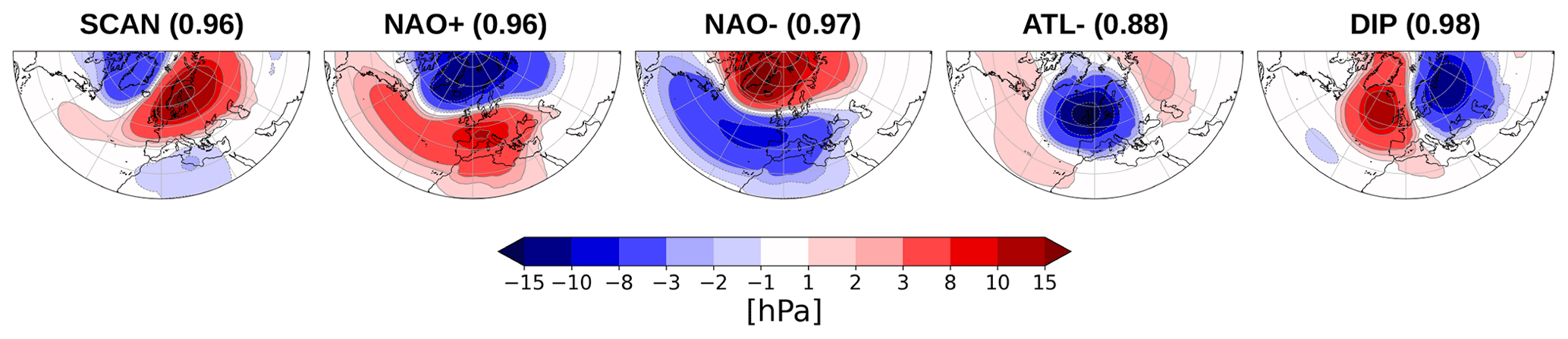
Figure 1Five circulation regimes over the Euro-Atlantic domain computed from daily ECHAM6 PAMIP slp anomaly data for the extended winter season (December, January, February, March). The computed regimes include a Scandinavian blocking pattern (SCAN), a positive and negative NAO-like pattern (NAO+ and NAO−), an Atlantic trough pattern (ATL−), and a dipole pattern (DIP). The numbers in parentheses show the pattern correlation coefficients of each pattern with the respective ERA5 pattern.
4.1.1 Regime structures
Figure 1 shows five circulation regimes computed for the extended winter season over the Euro-Atlantic domain. Daily slp anomaly data merged together from the ECHAM6 pdSIC and the futArcSIC simulation data have been used here. The computed regimes closely resemble regimes found in previous studies (e.g., Crasemann et al., 2017) and include a frequently detected Scandinavian blocking regime (Dorrington and Strommen, 2020; Falkena et al., 2020; Yiou et al., 2017), termed SCAN, with an anticyclonic blocking structure over Scandinavia and parts of the Ural Mountains. As shown in Fig. S6, up to 40 % of SCAN regime days are indeed accompanied by blocking activity over northern and northeastern Europe. Studies by for instance Jung et al. (2017) and Sato et al. (2014) showed that such an anticyclonic anomaly over northeastern Europe might be part of a wave train structure that originates from the east coast of North America and is forced by warming anomalies over this remote region. Another regime is characterized by a cyclonic structure over the Atlantic and parts of western Europe (ATL−) and has previously been named the negative Atlantic ridge (Falkena et al., 2020) or Scandinavian trough (Dorrington and Strommen, 2020). A dipole pattern (DIP) is found with positive pressure anomalies over the North Atlantic and negative pressure anomalies over northeastern Europe that has also been frequently termed the Atlantic ridge (Dorrington and Strommen, 2020; Falkena et al., 2020; Yiou et al., 2017). Finally, two of the computed regimes resemble the positive (NAO+) and negative (NAO−) phase of the North Atlantic Oscillation, respectively. The structure of the individual regimes is relatively unaffected by the exact definition of winter season (e.g., by excluding March) and by modifications of the spatial domain (using, e.g., 30 to 88∘ N, −80 to 80∘ W).
Compared to circulation regimes computed from ERA5 data (see Fig. S1 in the Supplement), it appears that ECHAM6 is able to realistically reproduce the spatial structure of these five regimes. Indeed, Fig. S3 indicates high spatial correlations (generally greater than 0.9) and similar (but, e.g., for NAO+ slightly higher) pattern amplitudes when comparing regimes computed from different combinations of ECHAM6 model simulations with ERA5 regimes.
In addition to ECHAM6 we also computed five circulation regimes for other PAMIP models. Figure S4 displays Taylor diagrams that compare regime patterns computed from the 11 different PAMIP models with the ERA5 regime structures. It shows that nine PAMIP models are able to realistically reproduce the ERA5 regimes pattern structures (pattern correlation averaged over all regimes greater than 0.8), whereas two models clearly stand out and show deficiencies in this respect (IPSL-CM6A-LR and FGOALS-f3-L). For the upcoming part of the analysis we only consider those nine PAMIP models that are able to realistically reproduce the ERA5 regime structures.
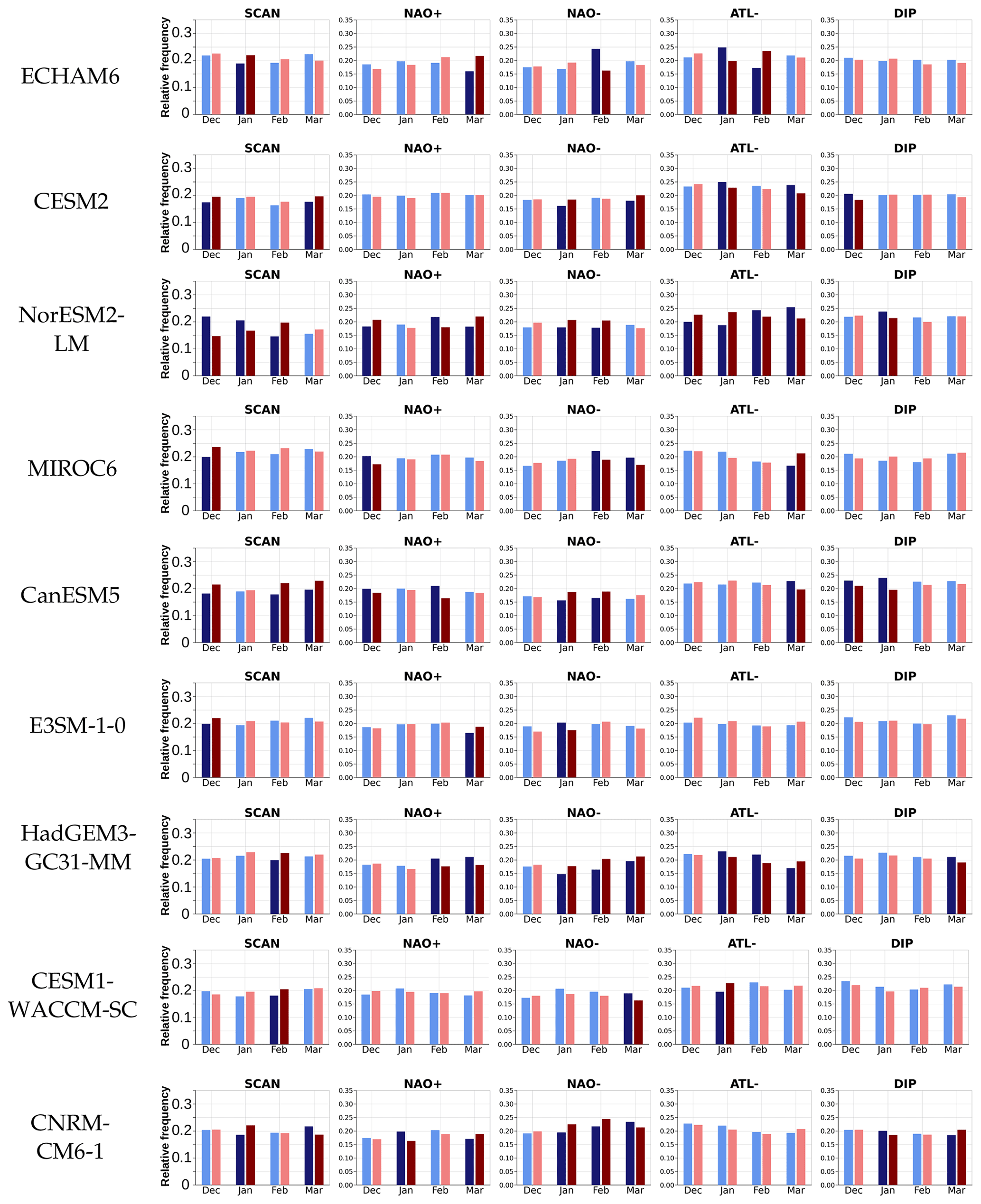
Figure 2Relative regime occurrence frequencies in different PAMIP models for different winter months compared between the pdSIC reference simulation (blueish bars) and the futArcSIC sensitivity simulation (reddish bars). Light reddish and blueish bars indicate non-significant frequency differences between reference and sensitivity simulations, whereas the paired dark blueish and reddish bars indicate significant differences in occurrence frequencies. Note that by definition the sum over all clusters for a specific month in a given simulation is 1. Only those nine PAMIP models that are, according to Fig. S4, able to realistically reproduce the ERA5 regime structures were considered here.
4.1.2 Regime frequency changes induced by future Arctic sea ice retreat
In order to assess the impact of future Arctic sea ice changes on the occurrence probability of certain regimes, Figs. 2 and S5 show monthly split histograms for different PAMIP models that compare the relative occurrence frequencies of computed circulation regimes between the reference simulation and futArcSIC (Fig. 2), as well as the futBKSIC sea ice sensitivity experiment (Fig. S5). Overall, it can be reported that regime frequency changes detected in the futArcSIC and futBKSIC sensitivity experiments of a specific model share similar features. Consistently with previous studies, this again emphasizes the potential key role of sea ice loss in the Barents and Kara sea region when trying to identify and understand linkages between the Arctic and mid-latitudes. We decided to analyze the regime occurrence for each winter month separately as proposed pathways underlying Arctic–mid-latitude teleconnections are often characterized by their evolution over the autumn–winter season (e.g., Kretschmer et al., 2016; Siew et al., 2020).
All nine models indicate a significant increase in SCAN occurrences in futArcSIC in at least 1 winter month, while in contrast only the NorESM2-LM and CNRM-CM6-1 models show significantly decreased SCAN occurrences (Fig. 2). A significant increase in SCAN occurrences in at least 1 winter month is detected in two out of five models for futBKSIC (Fig. S5). The respective months for which the SCAN response is detected generally differ between models. This may suggest that the underlying physical processes and pathways that lead to the occurrence of this SCAN increase are overall reasonably represented but that the onset and timing of such processes may differ between models. In general, this winter SCAN response is consistent with previous studies, such as by Luo et al. (2016), who related a strengthening of the Scandinavian or Ural blocking in winter season to instantaneous sea ice loss in the Barents–Kara sea region. Petoukhov and Semenov (2010) analyzed model simulations and showed that for moderate winter sea ice reductions over the Barents and Kara seas, an anticyclonic anomaly centered over the same region can be observed in February; however, they emphasized that such an anticyclonic circulation response depends on the actual prescribed magnitude of sea ice loss in the Barents and Kara seas in a highly nonlinear way. Within the framework of circulation regimes, Crasemann et al. (2017) detected an increased December SCAN occurrence frequency – although only in response to recent Arctic sea ice loss. It should be mentioned that a variety of recent modeling studies (Kim et al., 2022; Peings, 2019) did not find any intensifications of Ural blocking in response to sea ice loss over the Barents–Kara sea region.
Consistently with the recently reported weakening of mid-latitude westerly winds due to future sea ice loss in the PAMIP ensemble by Smith et al. (2022), five out of nine models in futArcSIC indicate preferred occurrences of the NAO− regime in at least 2 winter months (see Fig. 2). In contrast, decreased NAO− occurrences in at least 1 winter month can be detected in five models as well – including ECHAM6. Occurrence frequency changes of the NAO+ regime in futArcSIC also show pronounced discrepancies among different models, with four (five) models indicating an increased (decreased) NAO+ occurrence frequency in at least 1 winter month. Hence, we are overall not able to detect a robust NAO response under future sea ice loss in futArcSIC when comparing the different PAMIP models. For the futBKSIC experiment, three out of five models indicate decreased NAO+ and NAO− occurrences (see Fig. S5), which may suggest a weakened dominance of NAO variability under future sea ice loss in the Barents and Kara seas.
Although most models reveal significant frequency changes of the ATL− regime for futArcSIC and futBKSIC in different months, a consistent response among the different models can hardly be detected in any winter month. Occurrence frequencies of the DIP regime exhibit a significant decrease in five (two) out of nine (five) models in the futArcSIC (futBKSIC) experiment.
In order to later on demonstrate in Sect. 4.4 how such detected regime frequency changes can be employed to decompose sea-ice-induced changes in European temperature extremes, we finally briefly highlight the regime frequency changes detected in the ECHAM6 experiments (see Fig. S2). We will focus on only one model as a comprehensive interpretation of the upcoming decompositions for all nine models is very challenging and beyond the scope of this study. Indeed, ECHAM6 is one of the best of the models that are able to realistically reproduce the ERA5 regime structures (see Fig. S4). This additionally allows us to reasonably contrast the modeled ECHAM6 regime frequency changes with regime frequency changes between recent ERA5 conditions of low and high detrended Arctic sea ice (see triangles in Fig. S2). Conditions of low (high) detrended Arctic sea ice in ERA5 are defined as the lower (upper) 50 % of linearly detrended monthly averaged Arctic sea ice area anomalies over the period 1979–2018. Such an ERA5 analysis does not prove any causal link between recent sea ice loss and circulation regimes, and it does not isolate the effect of recent sea ice retreat. Nevertheless, we consider such ERA5 tendencies as additional statistical evidence, especially when deciding which of the significant ECHAM6 regime frequency changes are considered for the decompositions in Sect. 4.4.
In agreement with other PAMIP models, an overall midwinter increase in SCAN occurrence is detected in both ECHAM6 sea ice sensitivity simulation and the reanalysis (see Fig. S2a and f). Another significant signal found in both reanalysis and ECHAM6 is a more frequent occurrence of the ATL− pattern in January under higher-sea-ice conditions in the reference simulation (Fig. S2d and i). Lastly, especially the ECHAM6 futBKSIC sensitivity simulation reveals a decreased occurrence frequency of the NAO+ and NAO− pattern in February (Fig. S2g and h). The diminished occurrence frequency of the NAO+ pattern can be detected in the reanalysis as well.
4.2 Links between certain circulation regimes and European temperature extremes in ECHAM6
After examining how the occurrence probability of certain circulation regimes can be affected by sea ice changes, we now discuss which of the computed ECHAM6 circulation regimes can be associated with temperature extremes over Europe. For this reason, Fig. 3 compares the occurrence probability of temperature extremes given a specific circulation regime to the unconditioned probability of an overall extreme occurrence. Although this is only shown here for the ECHAM6 pdSIC reference simulation, results when using data from the sensitivity model experiments are qualitatively extremely similar. The general consistency with ERA5 (Fig. S9) suggests that for most European regions ECHAM6 is able to realistically represent the relevant physical processes that lead to the occurrence of temperature extremes during the respective regime days. Figure 3c indicates that the presence of an NAO− regime is associated with an up to more than doubled probability than usual of cold-extreme days over large parts of middle to northern Europe. This reported link between NAO− events and winter cold spells or negative temperature anomalies over northern Europe is well-established and frequently observed in studies (Cattiaux et al., 2010; Andrade et al., 2012; Rust et al., 2015; Screen, 2017b). Figure S8c shows how NAO− events are related to easterly zonal wind anomalies which consequently lead to favored cold-air advection of continental air masses towards northern Europe. These easterly anomalies can generally also be related to a suppressed advection of warmer maritime air masses, favoring colder conditions over Europe. As shown in Fig. S6b, up to 40 % of NAO− regime days are associated with atmospheric blocking activity over Greenland and the North Atlantic. Blocking conditions over these regions have previously been related to European winter cold spells as well (Sillmann et al., 2011).
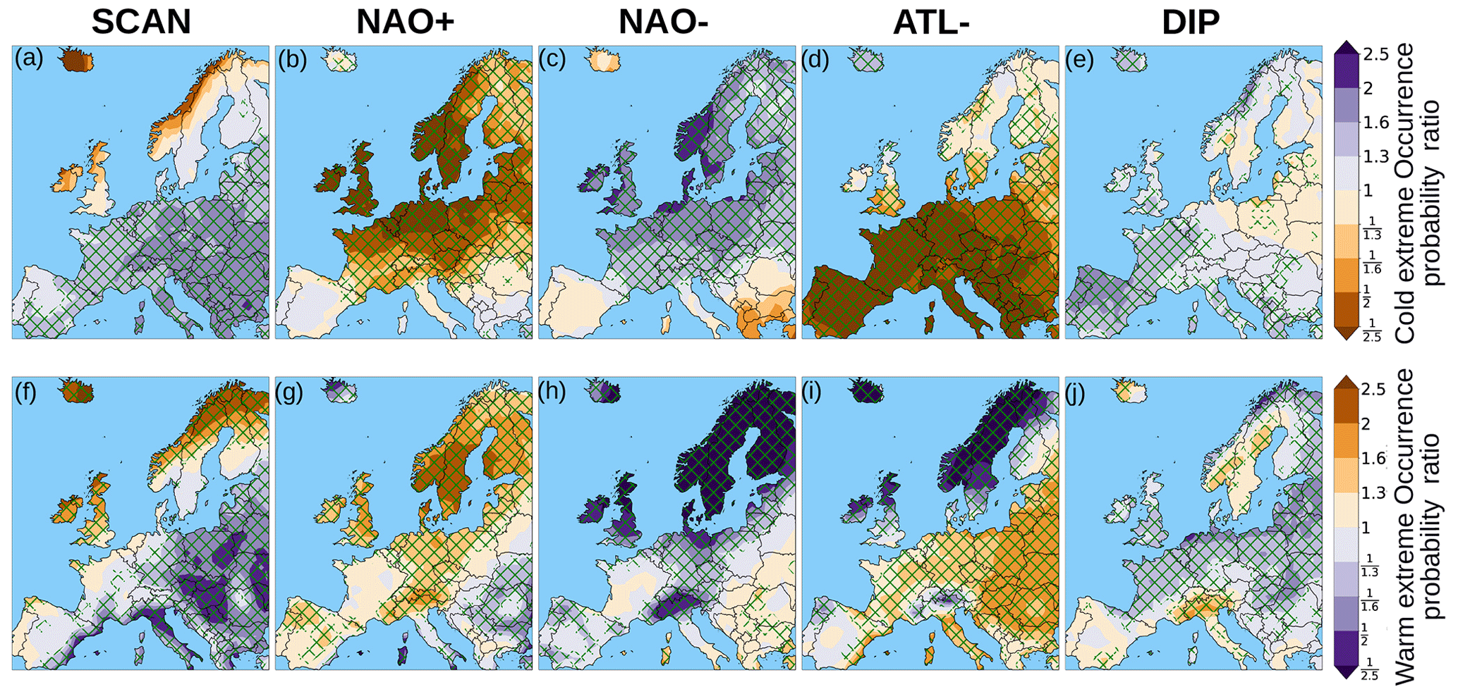
Figure 3Temperature extreme occurrence probability ratios averaged over the extended winter season for different circulation regimes plotted over the European domain using the ECHAM6 PAMIP pdSIC simulation. (a–e) Cold days. (f–j) Warm days. The plotted ratio compares the occurrence probability of an extreme day given a certain circulation regime to the unconditioned probability of an extreme occurrence. Thus, for instance violet values greater than 1 in (a–e) indicate a preferred cold-extreme occurrence at a specific grid point during the presence of a certain regime compared to the overall extreme occurrence. Note that the color bar is reversed for warm extremes in (f–j). Hatched areas indicate ratios that are significantly different from unity based on a moving bootstrap.
In addition to the NAO− regime, preferred occurrences of cold extremes over central and eastern Europe can be observed during SCAN days in Fig. 3a. Links between anticyclonic systems over Scandinavian and Ural regions and cold days over large parts of Europe have been reported previously (Petoukhov and Semenov, 2010; Andrade et al., 2012), since Scandinavian high-pressure systems are typically associated with cold-air advection towards central Europe from northeastern European regions (see Fig. S8a). Indeed, Lagrangian backward-trajectory analyses (Bieli et al., 2015) showed that cold events over middle and eastern Europe are induced by horizontal advection of air masses from Russia and far northeastern regions. These advective processes are furthermore characterized by an adiabatic and steady descent of the air masses. Additionally, Fig. 3e indicates preferred cold-extreme occurrences over most parts of western Europe during the presence of the dipole regime. This link is related to southward advection (see Fig. S8e) of Arctic air masses, especially from regions east of Greenland (Bieli et al., 2015).
Warm days in winter over large parts of central, eastern and southern Europe occur preferably during the presence of the ATL− regime (see Fig. 3i). As shown in Fig. S7a, around and westwards of the British Isles the ATL− regime is associated with enhanced baroclinic activity and consequently an intensification of the North Atlantic storm track. Therefore, more storm systems than usual may form and advect warm and moist Atlantic air masses towards middle and southern Europe. Complementarily, warm days over northern Europe are linked to the presence of the NAO+ regime (see Fig. 3g). Such warm extremes over northern Europe are linked to strengthened westerly transport of moist Atlantic air masses during positive NAO events, resulting in enhanced latent energy transport towards Scandinavia (Vihma et al., 2020). As shown in Fig. S7b this can also be related to a poleward shift of the North Atlantic storm track towards northern Europe and the Arctic.
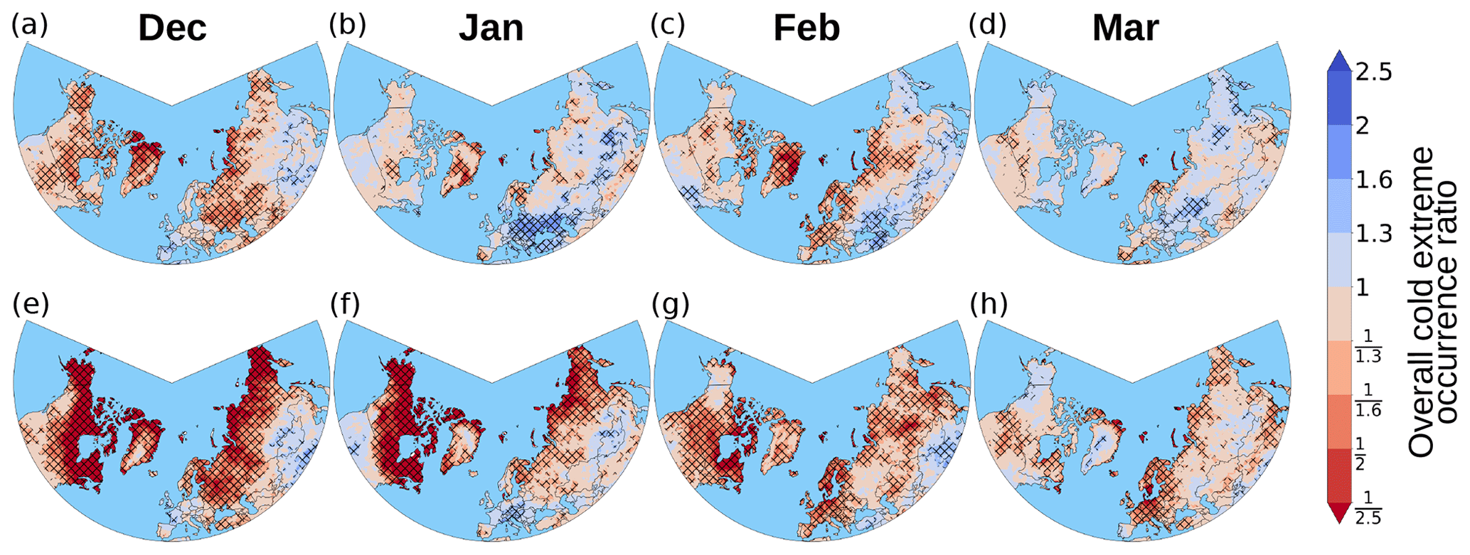
Figure 4Cold-extreme occurrence ratio for December, January, February and March in ECHAM6. The occurrence probabilities of northern hemispheric continental cold extremes are compared between the sensitivity experiments vs. the pdSIC reference simulation. Upper row (a–d): futBKSIC sensitivity run. Bottom row (e–h): futArcSIC sensitivity run. Blue indicates more frequent cold-extreme occurrences, and red indicates less frequent cold-extreme occurrences in the sensitivity experiments. Hatching indicates regions where the ratio differs significantly from unity based on a moving-block bootstrap.
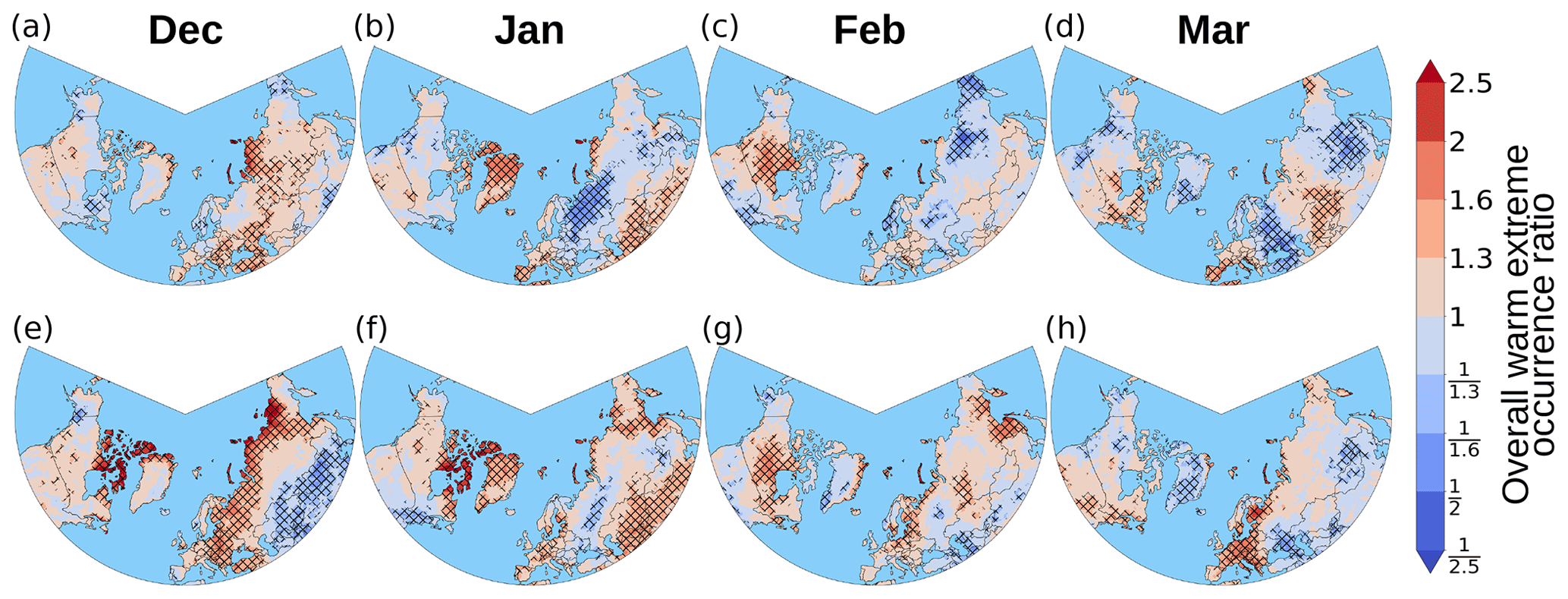
4.3 Sea-ice-induced changes in winter temperature extremes in ECHAM6
The upcoming section investigates the overall changes in occurrence frequencies of continental northern hemispheric winter temperature extremes, which can be expected under future Arctic sea ice loss in ECHAM6. Therefore, Figs. 4 and 5 depict the overall occurrence ratio ρ of cold and warm extremes, comparing the extreme occurrence probability in the futArcSIC and futBKSIC experiments with the reference simulation. Figure 4 indicates a general tendency towards less frequent cold-extreme occurrences in the future sea ice scenario simulations over the middle to high northern latitudes. From a thermodynamical perspective this observation is consistent with the fact that more open-water areas and the associated elevated surface temperatures in the sensitivity runs provide an additional energy source to the atmosphere. However, the spatial pattern and the signals' magnitude strongly depend on the specific month and whether sea ice is reduced over the entire Arctic (see Fig. 4e–h) or just over the Barents and Kara seas (see Fig. 4a–d). Although spatial tendencies show to some extent relatively similar patterns in both sensitivity simulations, futArcSIC exhibits much more pronounced reductions in cold extremes by a factor of more than 2.5 over high northern latitudes. In contrast, some parts over middle and northern Eurasia show more frequent cold-extreme occurrences in futBKSIC from January to March. This observation is consistent with the frequently reported Eurasian cooling response to sea ice loss in the Barents and Kara seas (Cohen et al., 2018) that has been associated with a strengthening of the Siberian High. Over Europe significant reductions in cold-extreme occurrences can be observed in futBKSIC in February (Fig. 4c), as well as in the futArcSIC simulation in February and March (Figs. 4g and h). Interestingly, January tends to exhibit slightly more cold extremes over central and eastern Europe in both sensitivity simulations (Fig. 4b and f).
As illustrated in Fig. 5 significant changes in the occurrence of warm extremes are generally less pronounced compared to cold extremes.
Over Europe an overall tendency towards more frequent occurrences of warm extremes can be detected, especially under conditions of diminished Arctic sea ice in the futArcSIC simulation (Fig. 5e–h). In many regions and months, reductions in cold-extreme occurrences are accompanied by increased probabilities of warm extremes. This might be associated with an overall thermodynamical shift of the underlying temperature distribution due to reduced sea ice concentrations and warmer surface temperatures in the sensitivity experiments. For futArcSIC this is, e.g., the case over northern Siberia in December (Figs. 4e and 5e) or over Europe in March (Figs. 4h and 5h). However, several regions such as central Europe in February show, for instance in futBKSIC, reductions in cold-extreme occurrences but no significant complementary changes in warm extremes (see Figs. 4c and 5c). Such asymmetric responses in the tails of the temperature distributions could be thermodynamically explained by a stronger warming of northerly polar winds compared to southerly winds as argued by Screen et al. (2014). Nevertheless, such responses could also be a result of other contributing factors, such as changes in the occurrence frequencies of atmospheric flows leading to certain extremes. In rare cases such as over central and eastern Europe in January, the futArcSIC experiment even shows an increased occurrence probability of both cold and warm extremes (see Figs. 4f and 5f). This might also be related to an overall increase in temperature variability.
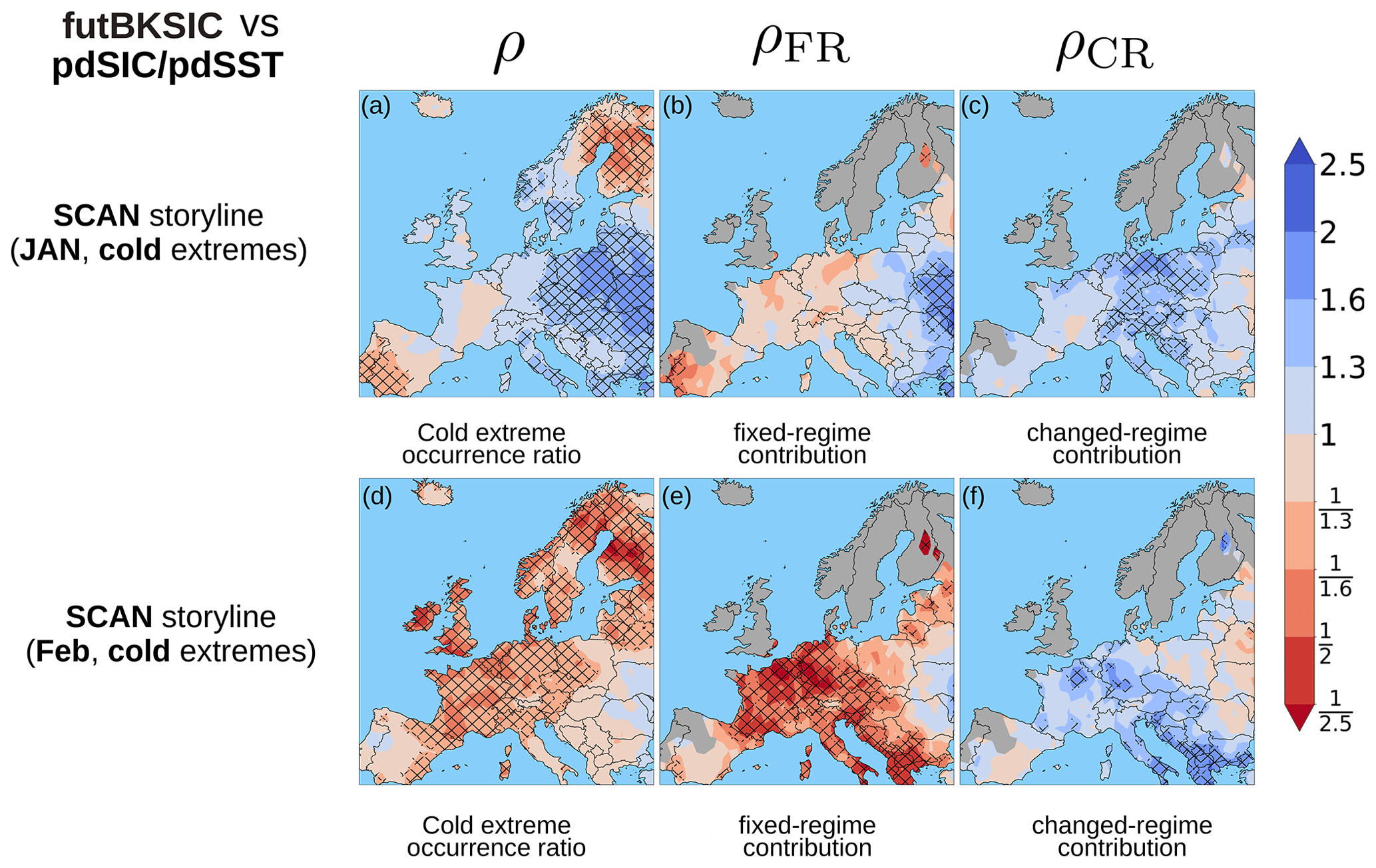
Figure 6Conditional extreme-event attribution framework for European cold extremes assuming a SCAN storyline. Compared are the futBKSIC sensitivity and the pdSIC reference simulations. Blue indicates more frequent cold-extreme occurrences, and red indicates less frequent cold-extreme occurrences in futBKSIC. (a–c) January with ρcirc = 1.26. (d–f) February with ρcirc = 1.23. ρcirc greater than unity means that the SCAN regime occurs more frequently in the futBKSIC simulation for both months (see also Fig. S2f). The first column shows the overall cold-extreme occurrence ratio between both simulations, the second column shows the fixed-regime contribution ρFR and the third one shows the changed-regime contribution ρCR. Hatching indicates regions where the ratios significantly differ from unity based on a moving-block bootstrap. ρFR and ρCR are only plotted for regions where statistically significant preferred winter cold-extreme occurrences during SCAN days are identified in Fig. 3a.
4.4 Decomposition of extreme frequency changes in ECHAM6
Now focus finally shifts back to temperature extremes over Europe. We try to understand to what extent sea-ice-induced changes in ECHAM6 extreme occurrences over Europe can be decomposed into fixed-regime and changed-regime contributions. Therefore, we now employ the conditional extreme-event attribution framework described in Sect. 3.2. On the one hand, in Sect. 4.1.2 we identified and compared significant regime frequency changes found in ECHAM6 with other PAMIP models and recently observed ERA5 tendencies. Based on these results and in order to discuss decompositions for different regime storylines, we focus on the SCAN, NAO+ and ATL− regime frequency changes in January and/or February. On the other hand, in Sect. 4.2 we discussed how these regimes can be statistically and dynamically related to preferred occurrences of European temperature extremes.
The following decompositions of overall responses in extreme occurrences are considered here for the futBKSIC simulation: European cold extremes along a SCAN storyline in January and February, warm extremes along an ATL− storyline in January, and warm extremes along an NAO+ storyline in February. Results for the futArcSIC simulation are shown in the Supplement and are also discussed below. Only months for which significant changes in regime occurrence frequencies have been detected in ECHAM6 (see Sect. 4.1) are considered here, since the physical interpretation of the changed-regime term ρCR strongly relies on significant changes in ρcirc. The decomposition method employed assumes that the presence of the respective reference regime Cref is necessary for an extreme to occur; hence, ρCR and ρFR are only plotted over regions where Fig. 3 indicates statistically significant, more frequent extreme occurrences during Cref.
Figure 6 shows the decomposition of the overall cold-extreme occurrence ratio ρ between the futBKSIC sensitivity simulation and the pdSIC reference experiment for January (Fig. 6a–c) and February (Fig. 6d–f). The SCAN regime was chosen as the reference pattern Cref, since it could be associated with cold extremes over central, western and eastern Europe (Fig. 3a) and revealed significant frequency changes in the midwinter months as well (Fig. S2f). In January it shows that eastern Europe and parts over central Europe are associated with significantly more frequent cold extremes in the futBKSIC simulation (Fig. 6a). The decomposition reveals that these signals can, especially over central Europe, be associated with a significant contribution of the changed-regime ρCR term (Fig. 6c). This contribution is related to a 26 % increase in SCAN regime occurrences in the futBKSIC simulation in January (see also Fig. S2f). Such a changed-regime contribution is however absent in more eastern parts of Europe, where the fixed-regime term ρFR significantly contributes to more frequent cold-extreme occurrences (Fig. 6b). ρFR compares the extreme occurrence probability during SCAN days. Hence, it cannot be ruled out that the individual daily flow patterns allocated to the SCAN regime change in a way that they more frequently promote the occurrence of southwestward cold-air advection towards eastern Europe and, thus, also the occurrence of cold extremes over this region.
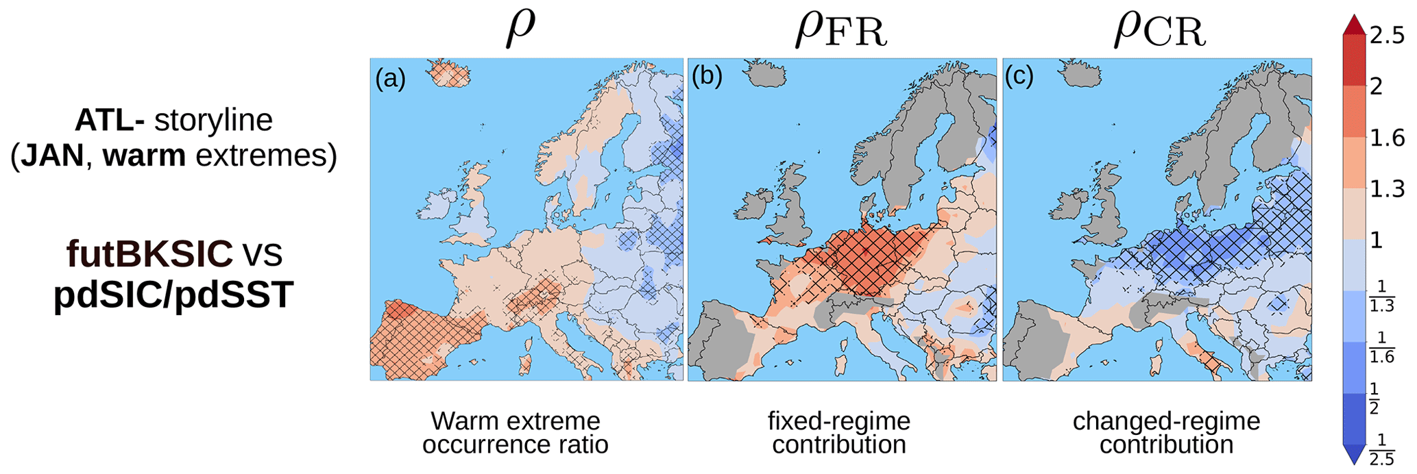
Figure 7Same as in Fig. 6 (futBKSIC vs. pdSIC simulation) but for January warm extremes and along an ATL− regime storyline. Compared to Fig. 6 the color bar is reversed such that red indicates more frequent warm-extreme occurrences and blue indicates less frequent warm-extreme occurrences in futBKSIC. The occurrence ratio of ATL− regime occurrence in January is given as ρcirc = 0.8. Thus, the ATL− occurs less frequently in the futBKSIC simulation (see also Fig. S2i). ρFR and ρCR are only plotted for regions where statistically significant preferred winter warm-extreme occurrences during ATL− days are identified in Fig. 3i.
In February, strong frequency decreases of cold extremes over large parts of western, central and northern Europe can be observed in the futBKSIC simulation (Fig. 6d). In contrast to January, the predominant part of these overall changes is explained by the fixed-regime term ρFR (Fig. 6e). This might be interpreted as an overall thermodynamical warming effect, since more ice-free areas in the model simulations are typically associated with warmer surface temperatures and with overall stronger ocean-to-atmosphere heat fluxes. Such additional heat and energy sources provided to the atmosphere are finally distributed via the climatological mean circulation. As air masses from northeastern Europe and the Barents and Kara seas frequently serve as source regions for advective processes leading to cold spells over central Europe (Bieli et al., 2015), an average warming of these reservoir regions may suppress the occurrence of cold extremes over Europe in the futBKSIC simulation. As it can be seen for the changed-regime term ρCR in Fig. 6f, February frequency changes in SCAN occurrences basically tend to favor cold extremes over most parts of Europe. However, compared to the fixed-regime term ρFR (Fig. 6e) these signals are relatively small and non-significant over most areas.
The same analysis for January is illustrated in Fig. S10 but considers the futArcSIC simulation instead of the futBKSIC simulation. The overall cold-extreme response (Fig. S10a) shows a significantly increased (decreased) probability of cold-extreme occurrences over some parts of central (northeastern) Europe. The increased cold-extreme probability over central Europe in Fig. S10a shows how two non-significant contributions (Fig. S10b and c) may add up to a significant overall response, whereas the decreased cold-extreme probability over northeastern Europe is mostly explained by the fixed-regime term ρFR (Fig. S10b).
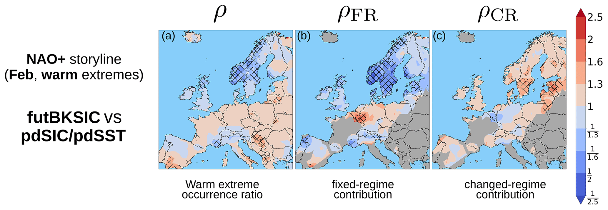
Figure 8Same as in Fig. 6 (futBKSIC vs. pdSIC simulation) but for February warm extremes and assuming an NAO+ regime storyline. Here, red indicates more frequent warm-extreme occurrences and blue indicates less frequent warm-extreme occurrences in futBKSIC. The occurrence ratio of NAO+ regime occurrence in February is given as ρcirc = 0.8. Thus, the NAO+ regime occurs less frequently in the futBKSIC simulation (see also Fig. S2g). ρFR and ρCR are only plotted for regions where statistically significant preferred winter warm-extreme occurrences during NAO+ days are identified in Fig. 3g.
Figure 7 shows the decomposition for European warm extremes in January, considering the ATL− regime as the reference pattern Cref. Here, the non-presence of significant signals in the overall warm-extreme occurrence ratio over most parts of Europe (Fig. 7a) is, especially over mid-Europe and parts of eastern Europe, a result of opposing ρFR (Fig. 7b) and ρCR (Fig. 7c) contributions. On the one hand, the reduced ATL− occurrence in the futBKSIC simulation can be associated with less frequent advection of warm air masses by Atlantic storm systems. On the other hand, an overall thermodynamical warming effect as mentioned before due to more open-water areas tends to favor the occurrence of warm extremes.
A similar line of reasoning for January warm extremes along an ATL− storyline can be used to interpret Fig. S11, where the futArcSIC simulation is considered and both contributions also appear to counteract each other. Here, an overall tendency towards more warm extremes can be observed over several parts of Europe compared to the futBKSIC simulation. This stems from a stronger dominance of the fixed-regime term ρFR (Fig. S11b), probably due to a more pronounced thermodynamical forcing for Arctic-wide sea ice loss compared to sea ice loss over the Barents and Kara seas only.
Figure 8 shows the decomposition for European warm extremes in February. The NAO+ regime is considered here the reference pattern Cref, since, on the one hand, it can be associated with warm extremes especially over more northern parts of Europe. On the other hand, it showed significantly less frequent occurrences in the futBKSIC simulation in February. The overall warm-extreme occurrence ratio ρ only shows some significantly less frequent extreme occurrences in the futBKSIC simulation over parts of Scandinavia (Fig. 8a). These signals are mostly explained by the fixed-regime contribution ρFR in Fig. 8b. In contrast, ρCR only shows a relatively small significant contribution (Fig. 8c).
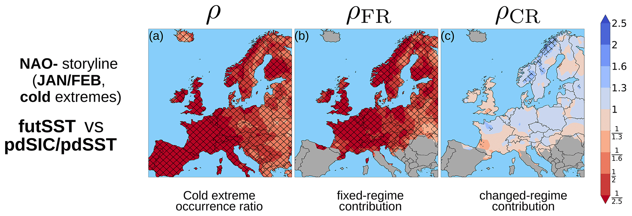
Figure 9Similar to Fig. 6 but comparing the pdSIC reference simulation and the futSST sensitivity simulation. Blue indicates more frequent cold-extreme occurrences, and red indicates less frequent cold-extreme occurrences in futSST. Analyzed are cold extremes in January–February, and an NAO− storyline is assumed here. ρFR and ρCR are only plotted for regions where statistically significant preferred winter cold-extreme occurrences during NAO− days are identified in Fig. 3c.
Finally, the previous results are contrasted to results for global SST changes in order to assess the relative importance of Arctic sea ice loss compared to a future increase in global SSTs. Therefore, Fig. 9 shows the overall response and the two contributions ρFR and ρCR for midwinter cold extremes comparing the ECHAM6 reference and the futSST simulation. The NAO− pattern was set as the reference pattern here. First, it shows that cold extremes occur massively and significantly less frequently in the futSST simulation over all parts of Europe (Fig. 9a). Secondly, these overall changes are almost completely explained by the fixed-regime term ρFR (Fig. 9b). Although in this case the NAO− regime only shows non-significant changes between both simulations (ρcirc=0.96), even significant and more distinct changes in regime occurrences could not contribute in the same way as the fixed-regime contribution. Figure 9 illustrates the decomposition of changes in extreme occurrences only for an NAO− storyline, but results for other storylines suggest the same qualitative picture: the thermodynamical impact of globally increased SSTs dominates dynamical impacts related to regime frequency changes, regardless of the chosen reference regime. A similar picture is found for warm extremes. Therefore, we can conclude that although future sea ice loss is able to affect extreme occurrences over Europe, compared to future SST increases and certainly also to future global warming, the effect is rather small.
The aims of this paper were, first, to discuss how future Arctic sea ice retreat is able to impact large-scale atmospheric dynamics in terms of occurrence frequency changes of Euro-Atlantic circulation regimes and, secondly, to demonstrate how such regime frequency changes can be employed to decompose sea-ice-induced frequency changes in European temperature extremes into a dynamically motivated changed-regime contribution and a more thermodynamically motivated fixed-regime contribution. Therefore, for the most part we investigated data from ECHAM6 sea ice sensitivity model experiments that are part of the PAMIP data pool. We considered simulations forced under future sea ice reduction over the entire Arctic, as well as only over the Barents and Kara seas, and compared them to a sensitivity simulation forced under present-day conditions.
Analyzing 10 additional PAMIP models, we initially studied how such future sea ice reductions affect the occurrence frequency of five Euro-Atlantic atmospheric circulation regimes that were computed with k-means clustering. Focusing on ECHAM6, we afterwards discussed which circulation regimes can be associated with cold or warm extremes over Europe and how the prescribed sea ice loss in the sensitivity simulations can impact the occurrence frequency of temperature extremes over the Northern Hemisphere. Based on the previous analysis steps, we employed a framework of conditional extreme-event attribution and decomposed the overall sea-ice-induced ECHAM6 extreme frequency changes over Europe along suitable regime storylines. The decomposition of changes in extreme-event frequencies finally yielded respective contributions, one changed-regime contribution related to changes in the atmospheric circulation (changes in regime occurrence frequencies) and another fixed-regime contribution that is related to increased surface temperatures during a specific atmospheric circulation regime.
The findings of the different analysis steps and research questions mentioned in the beginning can be summarized as follows:
-
Within the methodological framework of atmospheric circulation regimes, what changes in the wintertime atmospheric large-scale circulation over the Euro-Atlantic sector can be expected under future Arctic sea ice retreat? As already motivated by Crasemann et al. (2017), we also detected significant changes in the occurrence frequency of winter circulation regimes when contrasting idealized atmosphere-only model simulations forced under present-day and future Arctic sea ice conditions. Most PAMIP models revealed an increase in Scandinavian blocking (SCAN) occurrences under future Arctic sea ice conditions in different winter months. Despite the finding that consistently with recent studies several models indicated more frequent occurrences of an NAO− pattern under future sea ice loss in middle to late winter, an overall disagreement between individual models on the sign of frequency changes of NAO+ and NAO− regimes predominates.
-
Which regimes can be associated with preferred occurrences of winter temperature extremes over Europe? We showed and discussed that cold (warm) extremes over southern, central and eastern Europe occur significantly more frequently during SCAN (ATL−) days, whereas especially cold extremes over central to northern Europe are on average significantly more frequently associated with negative (positive) NAO regime events.
-
What overall frequency changes of extreme occurrences over the continental Northern Hemisphere can be detected in response to future sea ice changes in ECHAM6? We found that prescribed sea ice reductions in the ECHAM6 model simulations resulted in an overall tendency towards fewer cold-extreme days, especially over high northern continental regions. A general tendency towards more warm extremes was less clear. However, the signal structures and their signs as well as their significance levels highly depend on the specific region and month. Finally we noticed that reductions in cold-extreme occurrences are not necessarily accompanied by more frequent occurrences of warm extremes, and vice versa.
-
Based on the sea-ice-induced changes in circulation regimes detected in ECHAM6, to what extent can frequency changes of European extremes be related to fixed-regime and changed-regime contributions? The decomposition of overall responses of midwinter extreme occurrences in ECHAM6 revealed a rather complex picture. In several cases we could associate significant changed-regime contributions related to occurrence frequency changes of certain regimes with preferred or unfavored occurrences of extremes. This was especially the case for increased January cold extremes related to increased Scandinavian blocking occurrences or decreased January warm extremes related to a reduced frequency of the ATL− pattern. Furthermore, we observed in several cases that the fixed-regime contribution yielded from a thermodynamical point of view intuitively expected decreased (increased) occurrence frequencies of cold (warm) extremes under future sea ice conditions. Finally, we noticed different scenarios for the resulting overall extreme occurrence frequency response. First, one contribution may dominate and results in a significant overall response. This was for instance the case for February cold extremes following a SCAN storyline where the overall reduced extreme occurrence frequency is explained by the fixed-regime contribution. Secondly, changes in regime occurrences may counteract the fixed-regime warming or cooling trend, resulting in no detectable overall change in extreme occurrences. This was especially observed for January warm extremes following an ATL− storyline.
When analyzing changes in midwinter cold extremes induced by future raised global SSTs, we detected a strong and significant decrease in cold-extreme occurrences over all of Europe, especially when contrasted to results obtained for future sea ice reductions. Furthermore, this decrease was nearly completely explained by the fixed-regime contribution. This suggests a dominance of thermodynamical-warming arguments over changes in atmospheric dynamics when trying to understand future changes in European temperature extremes. Overall these findings indicate that although future Arctic sea ice loss is for sure able to affect temperature extremes over Europe and the related atmospheric dynamics, the total effect size compared to globally raised temperatures that are expected in the future is relatively small.
Finally, we want to outline some potential prospects for future studies, as well as some limitations regarding the interpretation of the results that may arise from the specific model setup, methodologies and sample sizes used in this study.
First, the presented analysis for ECHAM6 was conducted based on 100 ensemble members of 1-year-long time slice simulations for each respective experimental setup. In this respect, recent studies by Streffing et al. (2021), Peings et al. (2021) and Sun et al. (2022) have suggested that 100 ensemble members may not be enough to isolate the forced mean response from internal atmospheric variability in PAMIP sea ice sensitivity experiments. Furthermore, the results in Sect. 4.2–4.4 can differ for other PAMIP models, but conducting the decomposition method as applied in this study for each PAMIP model individually would be difficult; especially a comprehensive summary and interpretation of decomposition results for different models would be very challenging, in particular due to the fact that each model tends to simulate its distinct significant regime frequency changes in different months. Hence, the presented ECHAM6 analysis might be considered a first step and adapting the employed decomposition methodology for a feasible implementation into a multimodel analysis might provide a prospect for future studies.
The question to what extent the detected winter changes in extremes or circulation regimes are a result of time-delayed stratospheric pathways triggered by sea ice loss in autumn cannot be answered with the presented methodology and experimental design. From the experimental side this would require more tailored model experiments as for instance done by Blackport and Screen (2019). They compared the delayed effect of autumn and year-round sea ice loss on the winter circulation by using coupled model experiments with modified albedo parameters. When only studying model experiments with prescribed year-round sea ice loss, more dynamically based analyses (e.g., Jaiser et al., 2016) have to be conducted in order to assess the role of stratospheric pathways and autumn sea ice loss. This was however not the focus of the present study.
Furthermore, we investigated atmosphere-only model experiments that do not allow for a representation of atmosphere–ocean feedbacks. In this respect, previous studies have stressed the importance of an interactive ocean model (Screen et al., 2018). This may allow for representing additional oceanic pathways such as altered ocean currents that have been shown to amplify circulation responses to Arctic sea ice loss. However, in contradiction to this hypothesis, a recent study by England et al. (2022) shows that different approaches that impose sea ice perturbations in a coupled model setup add artificial heat to the Arctic region. This causes a spurious warming signal that is added to the warming expected from sea ice loss alone and therefore finally results in an overestimation of the climate response to sea ice retreat in coupled model setups.
The atmospheric response to sea ice loss also depends on the exact prescribed patterns of sea ice and SST boundary forcing (Screen, 2017a; McKenna et al., 2018) and the model used. Crasemann et al. (2017) for instance studied sea ice sensitivity simulations conducted with an atmospheric general circulation model (AGCM) for the Earth Simulator (AFES; Nakamura et al., 2015).
Compared to the experiments used in our study, their simulation data consisted of two perpetual runs over 60 years but forced under sea ice conditions averaged over the early 1980s and the early 2000s, respectively. Additionally, their SST background states were set to the early 1980s. With respect to circulation regime changes, they detected an increase in the Scandinavian blocking pattern under low-sea-ice conditions in December, as well as a more frequent occurrence of the NAO− pattern in February and March.
The five circulation regimes that were used throughout the study only provide coarse categorizations of the atmospheric flow and contain a variety of more specific synoptic patterns. In the case of European winter temperature extremes, we discussed that some of these large-scale variability patterns might be suitable to describe the typical atmospheric circulation during such extremes or at least contain most of the relevant synoptic patterns. The atmospheric situations during, e.g., spatially confined precipitation extremes, as well as summer heat waves that typically co-occur with an atmospheric ridge, may be too unique and uncommon to be examined and allocated to a certain large-scale circulation regime. An analogue approach might be more suitable for such extremes.
The framework of conditional extreme-event attribution employed in this study provides only one unique way to decompose atmospheric responses. The individual decompositions assume that the occurrence of a certain extreme can be completely associated with the presence of and changes in a certain circulation regime. Studies by Vautard et al. (2016) or Cassano et al. (2007) proposed for instance an approach where the individual contribution terms related to specific regimes add up to the overall response. However, Vautard et al. (2016) also showed very limited suitability of this methods when working with a very small number of circulation regimes.
Furthermore, it should be noted that within this study we only considered changes in the occurrence probability of extremes defined by a fixed threshold temperature in a present-day simulation. Similarly, changes in circulation regimes have also only been considered in terms of frequency changes. When aiming to draw conclusions about changes in the intensity and severity of extremes, other factors have to be taken account such as the actual strength of advection processes. Therefore, it might be helpful to distinguish between days that strongly (weakly) project onto a relevant pattern (e.g., NAO− for cold extremes) and are therefore connected to stronger (weaker) advective processes. This may provide an additional refinement possibility of the approach being employed in upcoming studies.
In conclusion, the present study provides a complementary and useful perspective on the question how future Arctic sea ice retreat can impact large-scale atmospheric dynamics, as well as to what extent European temperature extremes are affected by future Arctic sea ice loss and how these changes can be separated into dynamically and thermodynamically contributing factors.
Data from the different PAMIP models analyzed during the current study are available via the Earth System Grid Federation portal (https://esgf-data.dkrz.de/projects/cmip6-dkrz/, DKRZ, 2023). ERA5 reanalysis data are available via the Copernicus Climate Change Service (https://doi.org/10.24381/cds.adbb2d47, Hersbach et al., 2023).
The supplement related to this article is available online at: https://doi.org/10.5194/wcd-4-663-2023-supplement.
DH and JR developed the original idea for the paper. JR conducted the analysis and wrote the original draft. AR did the blocking frequency plots. AR, HR, UU and DH supervised and contributed to the interpretation of the results and provided feedback on the manuscript. TD did the ECHAM6 model simulation and also provided feedback on the manuscript.
The contact author has declared that none of the authors has any competing interests.
Publisher's note: Copernicus Publications remains neutral with regard to jurisdictional claims in published maps and institutional affiliations.
This article is part of the special issue “Past and future European atmospheric extreme events under climate change”. It is not associated with a conference.
Johannes Riebold, Dörthe Handorf, Andy Richling, Henning Rust and Uwe Ulbrich gratefully acknowledge the support by the ClimXtreme project, subproject ArcClimEx, funded by the German Ministry of Education and Research (grant nos. 01LP1901D (Johannes Riebold, Dörthe Handorf) and 01LP1901C (Andy Richling, Henning Rust, Uwe Ulbrich)). Dörthe Handorf was partly supported by the German Research Foundation (DFG, Deutsche Forschungsgemeinschaft) Transregional Collaborative Research Center SFB/TRR 172 “ArctiC Amplification: Climate Relevant Atmospheric and SurfaCe Processes, and Feedback Mechanisms (AC)3” (project ID 268020496) and by the European Union's Horizon 2020 Research and Innovation Framework Programme under grant agreement no. 101003590 (PolarRES). For his PAMIP-related work, Tido Semmler gratefully acknowledges support by the EU H2020 APPLICATE project (GA727862). Finally, the authors also want to acknowledge the Deutsches Klimarechenzentrum (DKRZ) in Hamburg for providing the general technical infrastructure for the analysis.
This research has been supported by the Bundesministerium für Bildung und Forschung (grant nos. 01LP1901D and 01LP1901C), the Deutsche Forschungsgemeinschaft (project ID 268020496) and Horizon 2020 (grant nos. 101003590 (PolarRES) and GA727862 (APPLICATE)).
This paper was edited by Gwendal Rivière and reviewed by Rym Msadek and one anonymous referee.
Andrade, C., Leite, S. M., and Santos, J. A.: Temperature extremes in Europe: overview of their driving atmospheric patterns, Nat. Hazards Earth Syst. Sci., 12, 1671–1691, https://doi.org/10.5194/nhess-12-1671-2012, 2012. a, b
Añel, J. A., Fernández-González, M., Labandeira, X., López-Otero, X., and de la Torre, L.: Impact of Cold Waves and Heat Waves on the Energy Production Sector, Atmosphere, 8, 209, https://doi.org/10.3390/ATMOS8110209, 2017. a
Barnes, E. A. and Screen, J. A.: The impact of Arctic warming on the midlatitude jet-stream: Can it? Has it? Will it?, WIREs. Clim. Change, 6, 277–286, https://doi.org/10.1002/wcc.337, 2015. a
Bieli, M., Pfahl, S., and Wernli, H.: A Lagrangian investigation of hot and cold temperature extremes in Europe, Q. J. Roy. Meteor. Soc., 141, 98–108, https://doi.org/10.1002/qj.2339, 2015. a, b, c
Blackport, R. and Screen, J. A.: Influence of Arctic Sea Ice Loss in Autumn Compared to That in Winter on the Atmospheric Circulation, Geophys. Res. Lett., 46, 2213–2221, https://doi.org/10.1029/2018GL081469, 2019. a
Blackport, R. and Screen, J. A.: Insignificant effect of Arctic amplification on the amplitude of midlatitude atmospheric waves, Sci. Adv., 6, eaay2880, https://doi.org/10.1126/sciadv.aay2880, 2020. a
Bolinger, R. A., Brown, V. M., Fuhrmann, C. M., Gleason, K. L., Joyner, T. A., Keim, B. D., Lewis, A., Nielsen-Gammon, J. W., Stiles, C. J., Tollefson, W., Attard, H. E., and Bentley, A. M.: An assessment of the extremes and impacts of the February 2021 South-Central U. S. Arctic outbreak, and how climate services can help, Weather. Clim. Extremes, 36, 100461, https://doi.org/10.1016/j.wace.2022.100461, 2022. a
Cassano, J. J., Uotila, P., Lynch, A. H., and Cassano, E. N.: Predicted changes in synoptic forcing of net precipitation in large Arctic river basins during the 21st century, J. Geophys. Res.-Biogeo., 112, G04S49, https://doi.org/10.1029/2006JG000332, 2007. a, b
Cattiaux, J., Vautard, R., Cassou, C., Yiou, P., Masson-Delmotte, V., and Codron, F.: Winter 2010 in Europe: A cold extreme in a warming climate, Geophys. Res. Lett., 37, L20704, https://doi.org/10.1029/2010GL044613, 2010. a, b, c
Chripko, S., Msadek, R., Sanchez-Gomez, E., Terray, L., Bessières, L., and Moine, M. P.: Impact of reduced arctic sea ice on Northern Hemisphere climate and weather in autumn and winter, J. Climate, 34, 5847–5867, https://doi.org/10.1175/JCLI-D-20-0515.1, 2021. a
Cohen, J., Furtado, J. C., Jones, J., Barlow, M., Whittleston, D., and Entekhabi, D.: Linking Siberian Snow Cover to Precursors of Stratospheric Variability, J. Climate, 27, 5422–5432, https://doi.org/10.1175/JCLI-D-13-00779.1, 2014. a, b
Cohen, J., Zhang, X., Francis, J., Jung, T., Kwok, R., Overland, J., Ballinger, T., Blackport, R., Bhatt, U. S., Chen, H., Coumou, D., Feldstein, S., Handorf, D., Hell, M., Henderson, G., Ionita, M., Kretschmer, M., Laliberte, F., Lee, S., Linderholm, H., Maslowski, W., Rigor, I., Routson, C., Screen, J., Semmler, T., Singh, D., Smith, D., Stroeve, J., Taylor, P. C., Vihma, T., Wang, M., Wang, S., Wu, Y., Wendisch, M., and Yoon, J.: Arctic change and possible influence on mid-latitude climate and weather, US CLIVAR reports, NCAR/UCAR, https://doi.org/10.5065/D6TH8KGW, 2018. a, b
Cohen, J., Zhang, X., Francis, J., Jung, T., Kwok, R., Overland, J., Ballinger, T. J., Bhatt, U. S., Chen, H. W., Coumou, D., Feldstein, S., Gu, H., Handorf, D., Henderson, G., Ionita, M., Kretschmer, M., Laliberte, F., Lee, S., Linderholm, H. W., Maslowski, W., Peings, Y., Pfeiffer, K., Rigor, I., Semmler, T., Stroeve, J., Taylor, P. C., Vavrus, S., Vihma, T., Wang, S., Wendisch, M., Wu, Y., and Yoon, J.: Divergent consensuses on Arctic amplification influence on midlatitude severe winter weather, Nat. Clim. Change, 10, 20–29, https://doi.org/10.1038/s41558-019-0662-y, 2020. a, b
Corti, S., Molteni, F., and Palmer, T. N.: Signature of recent climate change in frequencies of natural atmospheric circulation regimes, Nature, 398, 799–802, https://doi.org/10.1038/19745, 1999. a
Coumou, D. and Rahmstorf, S.: A decade of weather extremes, Nat. Clim. Change, 2, 491–496, https://doi.org/10.1038/nclimate1452, 2012. a
Crasemann, B., Handorf, D., Jaiser, R., Dethloff, K., Nakamura, T., Ukita, J., and Yamazaki, K.: Can preferred atmospheric circulation patterns over the North-Atlantic-Eurasian region be associated with arctic sea ice loss?, Polar Sci., 14, 9–20, https://doi.org/10.1016/J.POLAR.2017.09.002, 2017. a, b, c, d, e, f, g, h, i
Deser, C., Sun, L., Tomas, R. A., and Screen, J.: Does ocean coupling matter for the northern extratropical response to projected Arctic sea ice loss?, Geophys. Res. Lett., 43, 2149–2157, https://doi.org/10.1002/2016GL067792, 2016a. a
Deser, C., Terray, L., and Phillips, A. S.: Forced and internal components of winter air temperature trends over North America during the past 50 years: Mechanisms and implications, J. Climate, 29, 2237–2258, https://doi.org/10.1175/JCLI-D-15-0304.1, 2016b. a, b
Díaz, J., García, R., López, C., Linares, C., Tobías, A., and Prieto, L.: Mortality impact of extreme winter temperatures, Int. J. Biometeorol., 49, 179–183, https://doi.org/10.1007/S00484-004-0224-4, 2005. a
DKRZ: WCRP Coupled Model Intercomparison Project (Phase6) datasets, ESGF, https://esgf-data.dkrz.de/projects/cmip6-dkrz/ (last access: 27 January 2023), 2023. a
Dorrington, J. and Strommen, K. J.: Jet Speed Variability Obscures Euro-Atlantic Regime Structure, Geophys. Res. Lett., 47, e2020GL087907, https://doi.org/10.1029/2020gl087907, 2020. a, b, c, d
England, M. R., Eisenman, I., and Wagner, T. J. W.: Spurious Climate Impacts in Coupled Sea Ice Loss Simulations, J. Climate, 35, 3801–3811, https://doi.org/10.1175/jcli-d-21-0647.1, 2022. a, b
Falkena, S. K. J., de Wiljes, J., Weisheimer, A., and Shepherd, T. G.: Revisiting the Identification of Wintertime Atmospheric Circulation Regimes in the Euro-Atlantic Sector, Q. J. Roy. Meteor. Soc., 146, 2801–2814, https://doi.org/10.1002/qj.3818, 2020. a, b, c, d
Francis, J. A. and Vavrus, S. J.: Evidence linking Arctic amplification to extreme weather in mid-latitudes, Geophys. Res. Lett., 39, L06801, https://doi.org/10.1029/2012GL051000, 2012. a
Gervais, M., Atallah, E., Gyakum, J. R., and Bruno Tremblay, L.: Arctic air masses in a warming world, J. Climate, 29, 2359–2373, https://doi.org/10.1175/JCLI-D-15-0499.1, 2016. a
Handorf, D., Jaiser, R., Dethloff, K., Rinke, A., and Cohen, J.: Impacts of Arctic sea ice and continental snow cover changes on atmospheric winter teleconnections, Geophys. Res. Lett., 42, 2367–2377, https://doi.org/10.1002/2015GL063203, 2015. a
Hannachi, A., Straus, D. M., Franzke, C. L. E., Corti, S., and Woollings, T.: Low-frequency nonlinearity and regime behavior in the Northern Hemisphere extratropical atmosphere, Rev. Geophys., 55, 199–234, https://doi.org/10.1002/2015RG000509, 2017. a
He, S., Xu, X., Furevik, T., and Gao, Y.: Eurasian Cooling Linked to the Vertical Distribution of Arctic Warming, Geophys. Res. Lett., 47, e2020GL087212, https://doi.org/10.1029/2020GL087212, 2020. a
Hersbach, H., Bell, B., Berrisford, P., Hirahara, S., Horányi, A., Mu noz-Sabater, J., Nicolas, J., Peubey, C., Radu, R., Schepers, D., Simmons, A., Soci, C., Abdalla, S., Abellan, X., Balsamo, G., Bechtold, P., Biavati, G., Bidlot, J., Bonavita, M., Chiara, G., Dahlgren, P., Dee, D., Diamantakis, M., Dragani, R., Flemming, J., Forbes, R., Fuentes, M., Geer, A., Haimberger, L., Healy, S., Hogan, R. J., Hólm, E., Janisková, M., Keeley, S., Laloyaux, P., Lopez, P., Lupu, C., Radnoti, G., Rosnay, P., Rozum, I., Vamborg, F., Villaume, S., and Thépaut, J.: The ERA5 global reanalysis, Q. J. Roy. Meteor. Soc., 146, 1999–2049, https://doi.org/10.1002/qj.3803, 2020. a
Hersbach, H., Bell, B., Berrisford, P., Biavati, G., Horányi, A., Muñoz Sabater, J., Nicolas, J., Peubey, C., Radu, R., Rozum, I., Schepers, D., Simmons, A., Soci, C., Dee, D., and Thépaut, J.-N.: ERA5 hourly data on single levels from 1940 to present, Copernicus Climate Change Service (C3S) Climate Data Store (CDS) [data set], https://doi.org/10.24381/cds.adbb2d47, 2023. a
Hochman, A., Messori, G., Quinting, J. F., Pinto, J. G., and Grams, C. M.: Do Atlantic-European Weather Regimes Physically Exist?, Geophys. Res. Lett., 48, e2021GL095574, https://doi.org/10.1029/2021GL095574, 2021. a
Horton, D. E., Johnson, N. C., Singh, D., Swain, D. L., Rajaratnam, B., and Diffenbaugh, N. S.: Contribution of changes in atmospheric circulation patterns to extreme temperature trends, Nature, 522, 465–469, https://doi.org/10.1038/nature14550, 2015. a
Hoskins, B. and Woollings, T.: Persistent Extratropical Regimes and Climate Extremes, Curr. Clim. Change Rep., 1, 115–124, https://doi.org/10.1007/s40641-015-0020-8, 2015. a
Jaiser, R., Dethloff, K., Handorf, D., Rinke, A., and Cohen, J.: Impact of sea ice cover changes on the Northern Hemisphere atmospheric winter circulation, Tellus A, 64, 11595, https://doi.org/10.3402/tellusa.v64i0.11595, 2012. a
Jaiser, R., Nakamura, T., Handorf, D., Dethloff, K., Ukita, J., and Yamazaki, K.: Atmospheric winter response to Arctic sea ice changes in reanalysis data and model simulations, J. Geophys. Res.-Atmos., 121, 7564–7577, https://doi.org/10.1002/2015JD024679, 2016. a, b, c
Jung, O., Sung, M. K., Sato, K., Lim, Y. K., Kim, S. J., Baek, E. H., Jeong, J. H., and Kim, B. M.: How does the SST variability over the western North Atlantic Ocean control Arctic warming over the Barents-Kara Seas?, Environ. Res. Lett., 12, 034021, https://doi.org/10.1088/1748-9326/aa5f3b, 2017. a
Kim, S. H., Sung, H. J., Kim, S. J., Baek, E. H., Moon, J. Y., and Kim, B. M.: Contribution of Ural and Kamchatka Blockings to the Amplified Warm Arctic–Cold Eurasia Pattern under Arctic Sea Ice Loss and Eurasian Cooling, J. Climate, 35, 4071–4083, https://doi.org/10.1175/JCLI-D-21-0635.1, 2022. a
Kretschmer, M., Coumou, D., Donges, J. F., and Runge, J.: Using causal effect networks to analyze different arctic drivers of midlatitude winter circulation, J. Climate, 29, 4069–4081, https://doi.org/10.1175/JCLI-D-15-0654.1, 2016. a, b
Kunsch, H. R.: The Jackknife and the Bootstrap for General Stationary Observations, Ann. Stat., 17, 1217–1241, https://doi.org/10.1214/aos/1176347265, 1989. a
Labe, Z., Peings, Y., and Magnusdottir, G.: Warm Arctic, cold Siberia pattern: role of full Arctic amplification versus sea ice loss alone, Geophys. Res. Lett., 47, e2020GL088583, https://doi.org/10.1029/2020gl088583, 2020. a
Luo, D., Xiao, Y., Yao, Y., Dai, A., Simmonds, I., and Franzke, C. L.: Impact of ural blocking on winter warm Arctic-cold Eurasian anomalies. Part I: Blocking-induced amplification, J. Climate, 29, 3925–3947, https://doi.org/10.1175/JCLI-D-15-0611.1, 2016. a
MacQueen, J.: Some methods for classification and analysis of multivariate observations., in: Proc. 5th Berkeley Symp. in Mathematical Statistics and Probability, 21 June–18 July 1965, Berkeley, CA, USA, 1, 281–297, 1967. a
McKenna, C. M., Bracegirdle, T. J., Shuckburgh, E. F., Haynes, P. H., and Joshi, M. M.: Arctic Sea Ice Loss in Different Regions Leads to Contrasting Northern Hemisphere Impacts, Geophys. Res. Lett., 45, 945–954, https://doi.org/10.1002/2017GL076433, 2018. a
Meredith, M., Sommerkorn, M., Cassotta, S., Derksen, C., Ekaykin, A., Hollowed, A., Kofinas, G., Mackintosh, A., Melbourne-Thomas, J., Muelbert, M., Ottersen, G., Pritchard, H., and Schuur, E.: Polar Regions, in: IPCC Special Report on the Ocean and Cryosphere in a Changing Climate, edited by: Pörtner, H.-O., Roberts, D. C., Masson-Delmotte, V., Zhai, P., Tignor, M., Poloczanska, E., Mintenbeck, K., Alegria, A., Nicolai, M., Okem, A., Petzold, J., Rama, B. Weyer, N. N., Cambridge University Press, Cambridge, UK and New York, NY, USA, https://doi.org/10.1017/9781009157964.005, 203–320, 2019. a
Michelangeli, P.-A., Vautard, R., and Legras, B.: Weather regimes: Recurrence and quasi stationarity., J. Atmos. Sci., 52, 1237–1256, 1995. a
Nakamura, T., Yamazaki, K., Iwamoto, K., Honda, M., Miyoshi, Y., Ogawa, Y., and Ukita, J.: A negative phase shift of the winter AO/NAO due to the recent Arctic sea-ice reduction in late autumn, J. Geophys. Res.-Atmos., 120, 3209–3227, https://doi.org/10.1002/2014JD022848, 2015. a, b
Nakamura, T., Yamazaki, K., Iwamoto, K., Honda, M., Miyoshi, Y., Ogawa, Y., Tomikawa, Y., and Ukita, J.: The stratospheric pathway for Arctic impacts on midlatitude climate, Geophys. Res. Lett., 43, 3494–3501, https://doi.org/10.1002/2016GL068330, 2016. a
Notz, D. and SIMIP Community: Arctic Sea Ice in CMIP6, Geophys. Res. Lett., 47, e2019GL086749, https://doi.org/10.1029/2019GL086749, 2020. a
Otto, F. E.: Extreme events: The art of attribution, Nat. Clim. Change, 6, 342–343, https://doi.org/10.1038/nclimate2971, 2016. a
Palmer, T. N.: A nonlinear dynamical perspective on climate prediction, J. Climate, 12, 575–591, https://doi.org/10.1175/1520-0442(1999)012<0575:ANDPOC>2.0.CO;2, 1999. a, b
Peings, Y.: Ural Blocking as a Driver of Early-Winter Stratospheric Warmings, Geophys. Res. Lett., 46, 5460–5468, https://doi.org/10.1029/2019GL082097, 2019. a
Peings, Y., Labe, Z. M., and Magnusdottir, G.: Are 100 ensemble members enough to capture the remote atmospheric response to 12 ∘C arctic sea ice loss?, J. Climate, 34, 3751–3769, https://doi.org/10.1175/JCLI-D-20-0613.1, 2021. a
Petoukhov, V. and Semenov, V. A.: A link between reduced Barents–Kara sea ice and cold winter extremes over northern continents, J. Geophys. Res.-Atmos., 115, D21111, https://doi.org/10.1029/2009JD013568, 2010. a, b, c
Rantanen, M., Karpechko, A. Y., Lipponen, A., Nordling, K., Hyvärinen, O., Ruosteenoja, K., Vihma, T., and Laaksonen, A.: The Arctic has warmed nearly four times faster than the globe since 1979, Commun. Earth Environ., 3, 1–10, https://doi.org/10.1038/s43247-022-00498-3, 2022. a
Rayner, N. A., Parker, D. E., Horton, E. B., Folland, C. K., Alexander, L. V., Rowell, D. P., Kent, E. C., and Kaplan, A.: Global analyses of sea surface temperature, sea ice, and night marine air temperature since the late nineteenth century, J. Geophys. Res.-Atmos., 108, 4407, https://doi.org/10.1029/2002JD002670, 2003. a
Riboldi, J., Lott, F., D'Andrea, F., and Rivière, G.: On the Linkage Between Rossby Wave Phase Speed, Atmospheric Blocking, and Arctic Amplification, Geophys. Res. Lett., 47, e2020GL087796, https://doi.org/10.1029/2020GL087796, 2020. a
Rust, H. W., Richling, A., Bissolli, P., and Ulbrich, U.: Linking teleconnection patterns to European temperature – a multiple linear regression model, Meteorol. Z., 24, 411–423, https://doi.org/10.1127/METZ/2015/0642, 2015. a
Sato, K., Inoue, J., and Watanabe, M.: Influence of the Gulf Stream on the Barents Sea ice retreat and Eurasian coldness during early winter, Environ. Res. Lett., 9, 084009, https://doi.org/10.1088/1748-9326/9/8/084009, 2014. a
Savić, S., Selakov, A., and Milošević, D.: Cold and warm air temperature spells during the winter and summer seasons and their impact on energy consumption in urban areas, Nat. Hazards, 73, 373–387, https://doi.org/10.1007/S11069-014-1074-Y, 2014. a
Scaife, A. A. and Smith, D.: A signal-to-noise paradox in climate science, npj Clim. Atmos. Sci., 1, 1–8, https://doi.org/10.1038/s41612-018-0038-4, 2018. a
Screen, J. A.: Simulated Atmospheric Response to Regional and Pan-Arctic Sea Ice Loss, J. Climate, 30, 3945–3962, https://doi.org/10.1175/JCLI-D-16-0197.1, 2017a. a, b
Screen, J. A.: The missing Northern European winter cooling response to Arctic sea ice loss, Nat. Commun., 8, 1–9, https://doi.org/10.1038/ncomms14603, 2017b. a, b, c, d
Screen, J. A., Deser, C., Simmonds, I., and Tomas, R.: Atmospheric impacts of Arctic sea-ice loss, 1979-2009: Separating forced change from atmospheric internal variability, Clim. Dynam., 43, 333–344, https://doi.org/10.1007/s00382-013-1830-9, 2014. a
Screen, J. A., Deser, C., Smith, D. M., Zhang, X., Blackport, R., Kushner, P. J., Oudar, T., McCusker, K. E., and Sun, L.: Consistency and discrepancy in the atmospheric response to Arctic sea-ice loss across climate models, Nat. Geosci., 11, 155–163, https://doi.org/10.1038/s41561-018-0059-y, 2018. a
Shepherd, T. G.: A Common Framework for Approaches to Extreme Event Attribution, Curr. Clim. Change Rep., 2, 28–38, https://doi.org/10.1007/s40641-016-0033-y, 2016. a, b
Siew, P. Y. F., Li, C., Sobolowski, S. P., and King, M. P.: Intermittency of Arctic–mid-latitude teleconnections: stratospheric pathway between autumn sea ice and the winter North Atlantic Oscillation, Weather Clim. Dynam., 1, 261–275, https://doi.org/10.5194/wcd-1-261-2020, 2020. a, b
Sillmann, J., Mischa, C. M., Kallache, M., and Katz, R. W.: Extreme cold winter temperatures in Europe under the influence of North Atlantic atmospheric blocking, J. Climate, 24, 5899–5913, https://doi.org/10.1175/2011JCLI4075.1, 2011. a
Smith, D. M., Screen, J. A., Deser, C., Cohen, J., Fyfe, J. C., García-Serrano, J., Jung, T., Kattsov, V., Matei, D., Msadek, R., Peings, Y., Sigmond, M., Ukita, J., Yoon, J.-H., and Zhang, X.: The Polar Amplification Model Intercomparison Project (PAMIP) contribution to CMIP6: investigating the causes and consequences of polar amplification, Geosci. Model Dev., 12, 1139–1164, https://doi.org/10.5194/gmd-12-1139-2019, 2019. a, b, c, d
Smith, D. M., Eade, R., Andrews, M. B., Ayres, H., Clark, A., Chripko, S., Deser, C., Dunstone, N. J., García-Serrano, J., Gastineau, G., Graff, L. S., Hardiman, S. C., He, B., Hermanson, L., Jung, T., Knight, J., Levine, X., Magnusdottir, G., Manzini, E., Matei, D., Mori, M., Msadek, R., Ortega, P., Peings, Y., Scaife, A. A., Screen, J. A., Seabrook, M., Semmler, T., Sigmond, M., Streffing, J., Sun, L., and Walsh, A.: Robust but weak winter atmospheric circulation response to future Arctic sea ice loss, Nat. Commun., 13, 727, https://doi.org/10.1038/s41467-022-28283-y, 2022. a, b, c
Stevens, B., Giorgetta, M., Esch, M., Mauritsen, T., Crueger, T., Rast, S., Salzmann, M., Schmidt, H., Bader, J., Block, K., Brokopf, R., Fast, I., Kinne, S., Kornblueh, L., Lohmann, U., Pincus, R., Reichler, T., and Roeckner, E.: Atmospheric component of the MPI-M Earth System Model: ECHAM6, J. Adv. Model. Earth Sy., 5, 146–172, https://doi.org/10.1002/jame.20015, 2013. a
Straus, D. M., Corti, S., and Molteni, F.: Circulation Regimes: Chaotic Variability versus SST-Forced Predictability, J. Climate, 20, 2251–2272, https://doi.org/10.1175/JCLI4070.1, 2007. a
Streffing, J., Semmler, T., Zampieri, L., and Jung, T.: Response of Northern Hemisphere weather and climate to arctic sea ice decline: Resolution independence in polar amplification model intercomparison project (pamip) simulations, J. Climate, 34, 8445–8457, https://doi.org/10.1175/JCLI-D-19-1005.1, 2021. a
Stroeve, J. and Notz, D.: Changing state of Arctic sea ice across all seasons, Environ. Res. Lett., 13, 103001, https://doi.org/10.1088/1748-9326/AADE56, 2018. a
Sun, L., Deser, C., and Tomas, R. A.: Mechanisms of Stratospheric and Tropospheric Circulation Response to Projected Arctic Sea Ice Loss, J. Climate, 28, 7824–7845, https://doi.org/10.1175/JCLI-D-15-0169.1, 2015. a
Sun, L., Deser, C., Simpson, I., and Sigmond, M.: Uncertainty in the Winter Tropospheric Response to Arctic Sea Ice Loss: The Role of Stratospheric Polar Vortex Internal Variability, J. Climate, 35, 3109–3130, https://doi.org/10.1175/JCLI-D-21-0543.1, 2022. a
Trenberth, K. E., Fasullo, J. T., and Shepherd, T. G.: Attribution of climate extreme events, Nat. Clim. Change, 5, 725–730, https://doi.org/10.1038/nclimate2657, 2015. a
Vautard, R., Yiou, P., Otto, F., Stott, P., Christidis, N., Van Oldenborgh, G. J., and Schaller, N.: Attribution of human-induced dynamical and thermodynamical contributions in extreme weather events, Environ. Res. Lett., 11, 114009, https://doi.org/10.1088/1748-9326/11/11/114009, 2016. a, b, c
Vihma, T., Graversen, R., Chen, L., Handorf, D., Skific, N., Francis, J. A., Tyrrell, N., Hall, R., Hanna, E., Uotila, P., Dethloff, K., Karpechko, A. Y., Björnsson, H., and Overland, J. E.: Effects of the tropospheric large-scale circulation on European winter temperatures during the period of amplified Arctic warming, Int. J. Climatol., 40, 509–529, https://doi.org/10.1002/joc.6225, 2020. a
Yiou, P., Jézéquel, A., Naveau, P., Otto, F. E. L., Vautard, R., and Vrac, M.: A statistical framework for conditional extreme event attribution, Adv. Stat. Clim. Meteorol. Oceanogr., 3, 17–31, https://doi.org/10.5194/ascmo-3-17-2017, 2017. a, b, c, d, e, f, g, h