Spatial and temporal variability of the freezing level in Patagonia's atmosphere

The height of the 0 °C isotherm (H₀), which commonly signals the freezing level, denotes the lowest altitude within the atmosphere where the air temperature reaches 0 °C. This can be used as an indicator of the transition between rain and snow, making it useful for monitoring and visualizing the height of freezing temperatures in the atmosphere. We study the spatial and temporal variability of H₀ across Patagonia (41–54° S) for the 1959–2021 period using reanalysis data from ERA5. Our results indicate that the average isotherm in Patagonia is 1691 m above sea level (m a.s.l.). The spatial distribution of the annual mean field highlights the contrast in the region, with an average maximum of 2658 m a.s.l. in the north and minimum of 913 m a.s.l. in the south. Regarding seasonal variability in the region, H₀ ranges from 575 m a.s.l. (winter) to 3346 m a.s.l. (summer). Further, the significant trends calculated over the period show positive values in the whole area. This indicates an upward annual trend in the H₀, between 8.8 and 36.5 m per decade from 1959–2021, with the higher value observed in northwestern Patagonia. These upward trends are stronger during summer (8–61 m per decade). Empirical orthogonal function (EOF) analysis was performed on H₀ anomalies. The first EOF mode of H₀ variability accounts for 84 % of the total variance, depicting a monopole structure centred in the northwestern area. This mode exhibits a strong and significant correlation with the spatial average H₀ anomaly field (r=0.85), the Southern Annular Mode (SAM; r= 0.58), temperature at 850 hPa in the Drake Passage (r=0.56), and sea surface temperature off the western coast of Patagonia (r=0.66), underscoring the significant role of these factors in influencing the vertical temperature profile within the region. The spatial distribution of the second (8 %) and third (4.4 %) EOF modes depicts a dipole pattern, offering additional insights into the processes influencing the 0 °C isotherm, especially on the western slope of Patagonia.

1 Introduction

Patagonia, situated in the southern region of South America, is renowned for its distinct meteorological conditions and glaciers moulded by its geographical features (Aravena and Luckman, 2009; Bravo et al., 2022; Masiokas et al., 2020; Sauter, 2020). Spanning approximately 40 to 55° S, the austral Andes, reaching heights of around 1500 m above sea level (m a.s.l.), act as an obstacle that hinders the progress of moist tropospheric air masses originating from prevailing westerly winds (Garreaud et al., 2009).

The presence of this geographical barrier, along with the occurrence of baroclinic eddies, strong winds, and the influence of the Pacific Ocean, generates a significant climatic distinction between the western and eastern areas of Patagonia, leading to a pronounced precipitation gradient (Carrasco et al., 2002; Garreaud et al., 2013). These effects are mainly driven by the orographic ascent expansion and cooling of the air on the windward side, while in the leeward side precipitation is inhibited as descending air heats up, and any lingering liquid water evaporates (Lenaerts et al., 2014; Roe, 2005; Siler et al., 2013). Consequently, the western slopes receive substantial precipitation that exceeds 5000 mm yr⁻¹, fostering the growth of lush rainforests, rivers, and numerous glaciers. Conversely, the eastern slope exhibits a semi-arid steppe climate with a rain-shadow effect, receiving less than 1000 mm yr⁻¹ of precipitation (Garreaud et al., 2013; Lenaerts et al., 2014).

The climate of Patagonia is strongly influenced by modes of variability, where the Southern Annular Mode (SAM) is the primary driver of extratropical climate variability in the Southern Hemisphere (Marshall, 2003; King et al., 2023; Thomas et al., 2017; Hao et al., 2017). SAM significantly affects the westerly flow, shaping the atmospheric circulation patterns in the region. It is characterized by an equivalent barotropic, longitudinally symmetric structure that involves a mass exchange between the middle and high latitudes (Garreaud et al., 2009). SAM strengthens and shifts the polar jet stream poleward during its positive phase. This intensifies the westerly flow, leading to notable changes in temperature and precipitation patterns across Patagonia. Conversely, during its negative phase, SAM weakens and shifts the polar jet stream equatorward, impacting atmospheric circulation and influencing the region's climate. As a result, the variations in SAM play a crucial role in modulating the westerly flow and have significant implications. The circumpolar anomalies in westerly flow and tropospheric temperature observed during each phase of SAM result in corresponding anomalies in precipitation and surface temperature in Patagonia (Carrasco-Escaff et al., 2023). In the positive phase, higher temperatures and intensified westerly winds are present toward higher latitudes (Bravo et al., 2019; Fogt and Marshall, 2020). Conversely, the negative phase of SAM produces contrasting effects compared to those previously mentioned. During the latter half of the 20th century, SAM exhibited a positive trend, potentially influenced by anthropogenic factors (ozone depletion and increase in greenhouse gases), which could have implications for future climate patterns (Abram et al., 2014; Fogt and Marshall, 2020).

Carrasco-Escaff et al. (2023) elucidate another key atmospheric system in the region, called the Drake Low, which exhibits anomalies in cyclonic circulation around the Drake Passage. These anomalies extend longitudinally from the Amundsen Sea to the northeastern part of the Antarctic Peninsula and latitudinally from the western Antarctic coast to the southernmost tip of South America (designated as the R1 area). The presence of the Drake Low intensifies westerly winds, which notably affects the Patagonian region. This intricate system operates through a thermodynamic mechanism facilitated by a core of cold air, playing an active role in cooling the Patagonian region during the summer months. The study's findings provide valuable insights into the complex interplay between large-scale atmospheric dynamics and their direct influence on regional climate patterns.

Revisiting the distinctive attributes of the region, the Northern and Southern Patagonian icefields, which encompass the largest glacier area in Patagonia, play an important role in the local and regional environment (Dussaillant et al., 2012). Recent research underscores their significant contribution to the rise in sea level compared to other ice masses in South America (Malz et al., 2018; Masiokas et al., 2020; Minowa et al., 2021) and the increasing loss of mass over the past few decades (Hugonnet et al., 2021). The sustained atmospheric warming has a profound impact on the mass balance of glaciers (Van der Geest and Van den Berg, 2021), especially in terms of the height of the 0 °C isotherm (Schauwecker et al., 2017). Changes in this variable results in changes in the snow accumulation rates, amplified melting, and heightened flow rates during moderate or extreme precipitation events, such as atmospheric rivers (Saavedra et al., 2020). This, in turn, renders the region more susceptible to natural hazards, including an increased risk of floods (Somos-Valenzuela et al., 2020), landslides, and glacial lake outburst floods (Iribarren-Anacona et al., 2015; Mardones and Garreaud, 2020). Nonetheless, the limited availability of data and analysis (particularly at the highest elevations) has hindered our comprehensive understanding of the fundamental mechanisms governing the interaction between these variables and the freezing level, especially the large-scale climate processes operating on different timescales.

This study aims to assess and quantify the patterns and variations in H₀ in Patagonia. In the first section, we estimate the freezing-level values based on ERA5 reanalysis data (climate-gridded product), which were validated with observed data from four radiosonde stations. Next, we analyse spatial pattern, seasonal and annual cycles, trend, and interannual variability using reanalysis data from 1959–2021. The Discussion section addresses the reanalysis limitations, spatio-temporal distribution, large-scale drivers, and their implications.

2 Data and methods

2.1 Study area

Our research focuses on a vast expanse of Patagonia, delineated by a red rectangle in Fig. 1a. This region spans latitudes from 41 to 54° S and longitudes from 78 to 66° W, encompassing small fractions of both the Pacific and the Atlantic oceans. The selection of this domain was guided by the locations of radiosonde stations, specifically Puerto Montt (northwest, at 84 m a.s.l.), Comodoro Rivadavia (northeast, at 58 m a.s.l.), Río Gallegos (southeast, at 20 m a.s.l.), and Punta Arenas (south, at 38 m a.s.l.). Despite potential limitations posed to the west by Puerto Montt station (as a border domain point), we extended the area toward the west (78° W) to include a significant portion of western Patagonia and the Pacific coast. Moreover, this longitudinal range encompasses the austral Andes (AA) and the glaciers of the Northern and Southern Patagonian icefields.

Figure 1 (a) Topographic map of South America highlighting key features in the Patagonia region. Terrain elevation (m a.s.l.) was acquired from the ETOPO1 model with 1 arcmin resolution. The red rectangle indicates the study region of Patagonia. The dots indicate the locations of the radiosonde stations of Puerto Montt (orange), Comodoro Rivadavia (red), Río Gallegos (blue), and Punta Arenas (purple). (b) The coloured areas represent the regions used for the construction of custom climate indices.

2.2 Assessment of isotherm at 0 °C

Two sets of data were used to estimate the free tropospheric values of the 0 °C isotherm. The first corresponds to ERA5 reanalysis data (Hersbach et al., 2020). This reanalysis comprises a latitude–longitude grid with a spatial resolution of 0.25° × 0.25°, encompassing 37 pressure levels. For our analysis, we utilize the hourly data from 1959 to 2021. Then, we extract vertical profiles of air temperature and geopotential height, spanning levels from the surface up to 400 hPa. Each profile is analysed to identify the temperature transition above and below 0 °C. ERA5 freezing-level values ($H_{\mathrm{0}}^{\mathrm{ERA}\mathrm{5}}$) are determined by linear interpolation between the geopotential heights corresponding to the transition levels. If multiple elevations of 0 °C are found, for instance, from temperature inversions, the lowest value is assigned. Additionally, if no zero crossing levels are found, the corresponding value is flagged as missing. To obtain a representative value per day, we calculate the daily average of $H_{\mathrm{0}}^{\mathrm{ERA}\mathrm{5}}$ (H₀ – daily average, Fig. 2) using five values (00:00, 06:00, 12:00, 18:00, 24:00 UTC). This approach ensures that we capture the diurnal variability and provide a comprehensive picture of the freezing level throughout the day. We utilized a second dataset comprising observations from radiosonde stations. We applied the proposed methodology to estimate the radiosonde freezing-level values ($H_{\mathrm{0}}^{\mathrm{IGRA}}$), allowing us to validate the freezing-level values obtained from ERA5 at specific locations. These observed values were obtained from the Integrated Global Radiosonde Archive (IGRA) product (Durre et al., 2018). With this data, we implemented an additional criterion, specifically utilizing vertical profiles that included a minimum of three data points. Vertical profiles with inadequate data were excluded from the analysis. Fourth locations with comparable recording periods were selected for analysis: Puerto Montt, Comodoro Rivadavia, Río Gallegos, and Punta Arenas (Fig. 1). The selection criteria for these locations were established to include only those with a minimum of a decade's worth of data, excluding other locations that do not meet this criterion. We compared the grid's closest point of $H_{\mathrm{0}}^{\mathrm{ERA}\mathrm{5}}$ to $H_{\mathrm{0}}^{\mathrm{IGRA}}$, and only 12Z data were used to assess the agreement between them. Only this hour was selected since it has a greater number of observations in the records. The outcomes of this process are summarized in Table 1, where the Pearson correlation, root mean square error (RMSE), standard deviation, and average were estimated in selected periods for each location.

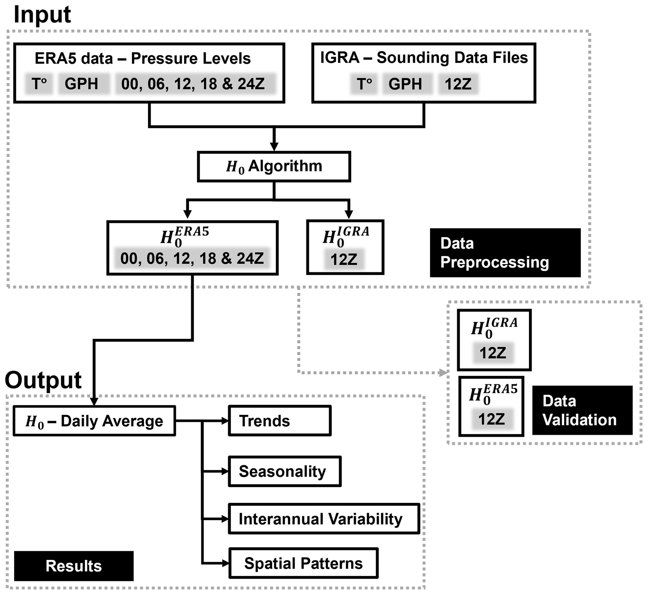
Figure 2 The data processing workflow for H₀ between 1959 and 2021. Two distinct sets of input data were utilized: one comprising reanalysis data and the other containing radiosonde observations. The isotherm 0 °C values were derived from these datasets, and a validation process was employed. Daily values were computed based on the reanalysis data.

Table 1 Data and statistics of the validation process between daily values of ${\mathrm{H}}_{\mathrm{0}}^{\mathrm{IGRA}}$ and ${\mathrm{H}}_{\mathrm{0}}^{\mathrm{ERA}\mathrm{5}}$. The first columns indicate the latitude (lat), longitude (long), period, and number of data available (n_obs). Other columns depict statistics as the Pearson correlation (r^*, values that are statistically significant at a p value < 0.05), mean values (${\stackrel{\mathrm{‾}}{H}}_{\mathrm{0}}$), standard deviation (σ₀), mean bias error (MBE), and root mean square error (RMSE).

2.3 Indices and trends

To analyse large-scale patterns associated with H₀, we followed the methodology of the NOAA Climate Prediction Center (https://www.cpc.ncep.noaa.gov/products/precip/CWlink/daily_ao_index/history/method.shtml, last access: 10 January 2024) to construct the SAM index. This index is derived by projecting 700 hPa geopotential height anomalies onto the loading pattern of SAM, which is defined as the leading empirical orthogonal function (EOF1) of the monthly mean at the 700 hPa geopotential height anomalies from 20° S poleward during the period of 1959–2021 (Shi et al., 2019). For more details, see the teleconnection pattern calculation procedures from NOAA's Climate Prediction Center (CPC) (https://www.cpc.ncep.noaa.gov/products/precip/CWlink/daily_ao_index/history/method.shtml, last access: 10 January 2024). Anomalies are computed relative to the corresponding month's mean over the same period. To ensure equal area weighting in the covariance matrix, the gridded data are weighted by the square root of the cosine of latitude. Moreover, we performed spatial averaging of monthly ERA5 values for specific areas and variables, following the methodology outlined by Carrasco-Escaff et al. (2023), with the exception that we used standardized indices. In Fig. 1b, the R1 box represents the geopotential height at 300 hPa and air temperature at 850 hPa near the Drake Passage (68–53° S, 100–60° W). The R2 box represents the southeastern Pacific sea surface temperature (SST) adjacent to central Patagonia (52.5–41° S, 80–76° W). Lastly, the R3 box represents the zonal wind at 850 hPa impacting central Patagonia (52.5–41° S, 75.5–74.5° W). These time series are labelled R1-Z300, R1-T850, R2-SST, and R3-U850, respectively. Our objective is to comprehend the similarities between the regions and the influences that these regions and variables may exert on the temperature profile within the area. Trend values of H₀ are estimated, which are derived from the Mann–Kendall test and Theil–Sen estimator (Wilks, 2019; Hussain et al., 2019). A trend was considered statistically significant if the p value < 0.05. A summarized scheme of the methodology implemented is presented in Fig. 2.

3 Results

3.1 Validation

The statistical analysis between pairs of time series is presented in Table 1 and Fig. 3. The results unveil significant relationships among the variables under investigation. Notably, the freezing level in Puerto Montt, Comodoro Rivadavia, Río Gallegos, and Punta Arenas demonstrates a consistently strong positive correlation throughout the entire period (r= 0.97, 0.96, 0.8, and 0.94, respectively).

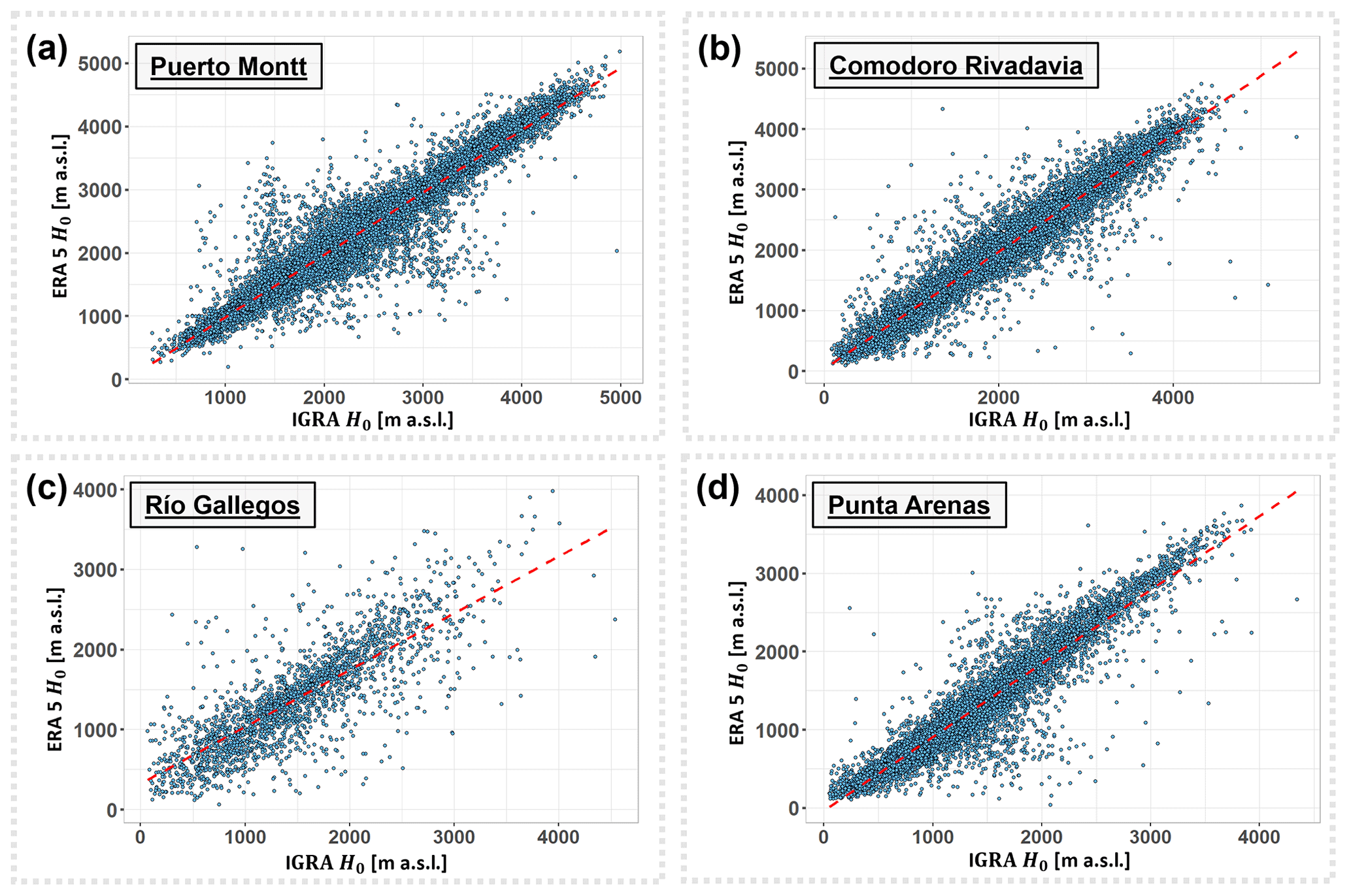
Figure 3 Scatterplots from Puerto Montt (a), Comodoro Rivadavia (b), Río Gallegos (c), and Punta Arenas (d). The reference data correspond to ${\mathrm{H}}_{\mathrm{0}}^{\mathrm{ERA}\mathrm{5}}$ (closest grid point) and ${\mathrm{H}}_{\mathrm{0}}^{\mathrm{IGRA}}$. The dotted red line in the scatterplots shows the 1:1 line.

$H_{\mathrm{0}}^{\mathrm{ERA}\mathrm{5}}$ effectively captures the southern thermal gradient within the study area. This pattern becomes apparent when examining the decreasing average heights of $H_{\mathrm{0}}^{\mathrm{ERA}\mathrm{5}}$ from Puerto Montt (2278 ± 980 m a.s.l.) to Punta Arenas (1176 ± 655 m a.s.l.). The noticeable disparity between the averaged isotherms for the northern and southern points of the study area further reinforces this point.

The mean bias error (MBE) between $H_{\mathrm{0}}^{\mathrm{ERA}\mathrm{5}}$ and $H_{\mathrm{0}}^{\mathrm{IGRA}}$ values is negative at each comparison point, indicating an underestimation of the freezing-level height by the ERA5 reanalysis. The smaller MBEs were estimated in the northern zone, reaching an absolute minimum of 30 m a.s.l. in Comodoro Rivadavia, followed by Puerto Montt with 36 m a.s.l. The larger biases were obtained for the southernmost zone, reaching an absolute maximum of 111 m a.s.l. in Punta Arenas, closely followed by Río Gallegos at 107 m a.s.l. The calculated standard deviation for each pair of points was remarkably similar. The root mean square error for the longest series (Puerto Montt and Comodoro Rivadavia) ranges from 240–252 m a.s.l. For Río Gallegos, which has the smallest number of observations (barely a decade), the root mean square error increases to 445 m a.s.l. Despite this increase, the average value of the data is not exceeded by the RMSE in any of the cases, which indicates that the uncertainty is contained in the means of the data. For more details and calculations using the observations, refer to the supplementary material section. Additional results from the comparison of observed and reanalysis data are provided in the Supplement (Tables S1 and S2).

3.2 Spatial patterns of H₀

The annual average of the H₀ field in the zone reveals a north-to-south variation, with higher height in the northern region and lower height in the southern region (Fig. 4). The latitudinal profile (Fig. 4b) shows a gradual decrease, intersecting with the topography between 47–51° S. The interquartile range in the latitudinal profile (IQR_m) fluctuates from 905 to 2626 m a.s.l. and captures the extent of the variations within the highest levels of the topography.

Figure 4 (a) Spatial distribution of the annual average of H₀. The lighter areas depict a lower height of H₀, while the red areas indicate higher values. The white contours delineate the extent of ice coverage in the region. Each distribution is accompanied by a (b) latitudinal profile and (c) a longitudinal profile, showcasing the spatially averaged H₀ values. The purple-shaded area in these profiles represents the respective interquartile range for each profile (IQR_m,z). The grey contours illustrate topographic profiles corresponding to the 2.5th percentile (dark grey) and 97.5th percentile (light grey).

Conversely, the longitudinal profile (Fig. 4c) exhibits an abrupt change in H₀ between 70–74° W, coinciding with the presence of the highest peaks of the AA. The zone exhibits a broad range in the longitudinal interquartile range (IQR_z) ranging from 705 to 2654 m a.s.l., indicating significant variability in H₀, which surpasses that of IQR_m. Moreover, IQR_z encompasses the freezing level's proximity to the lowest topography on the western side of the area. In the eastern region, IQR_z approaches H₀ only at the highest topography on the eastern side. Spatially, the region demarcated by higher isotherms forms a ridge, with its axis extending over the eastern side. In contrast, lower isotherms delineate a trough, with its axis extending over the western side. Notably, the difference between the western and eastern sides of H₀ occurs above the highest section of the AA, from around 70 to 74° W (Fig. 4c). To simplify and establish a clear transition zone between the western and eastern sides of H₀, we designate 72° W as the boundary longitude.

Consequently, we used this meridian as a reference for a transitional boundary in the AA (Fig. 4), demarcating a middle ground where various regional geographical features converge. In doing so, we define western Patagonia as the region situated west of the 72° W meridian, while eastern Patagonia lies east. We used this definition to contrast the H₀ values in a histogram, analysing the values across all of Patagonia, the western zone, and the eastern zone from 1959 to 2021 (Fig. 5). The histogram indicates that the average and median values for the entire region are 1691 and 1519 m a.s.l., respectively (Table S3). Since the median is lower than the mean, the distribution shows positive skewness or is right skewed. Additionally, the upper extreme values (95th percentile) reach 3424 m a.s.l., while the lower extreme values (5th percentile) are around 488 m a.s.l. (Fig. S1). A clear contrast in the H₀ distribution between western Patagonia (blue line) and eastern Patagonia (red line) can be observed. Western Patagonia has a lower height, indicated by a higher frequency of lower H₀ values, with an average and median reaching 1568 and 1347 m a.s.l., respectively. On the other hand, eastern Patagonia shows a higher frequency of relatively higher values, with an average and median of 1818 and 1708 m a.s.l., respectively. The two regions differ by approximately 251 m a.s.l. (mean) to 362 m a.s.l. (median) for the entire period. These values are shown in the supplementary material (Fig. S1).

Figure 5 Histogram of daily simulated 0 °C isotherm height in Patagonia. The grey bars represent the daily values of H₀ obtained from the spatial average across the entire study area from 1959 to 2021. The curves, on the other hand, indicate the fit of the kernel density estimation for the entire region (grey), western Patagonia (blue), and eastern Patagonia (red).

3.3 Seasonal cycle of H₀

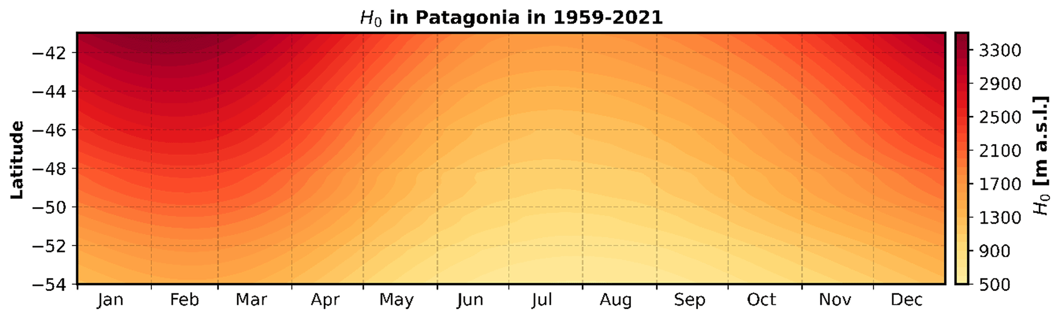
The average variations in H₀ from north to south exhibit a marked seasonality (Fig. 6). During the summer months, a distribution with higher heights is observed, reaching peak values in mid-summer (January–February) over the region. From March, there is a sustained decrease in H₀, reaching its lowest point during winter (July–August). The estimated mean amplitude indicates a range between 575 and 3346 m a.s.l. (the highest absolute average in summer and winter). The average annual difference between the northernmost and southernmost zones of our study area is 1511 m a.s.l.

Figure 6 Latitudinal profile of daily climatology of H₀ in Patagonia from 1959 to 2021.

A detailed examination of the seasonal averages provides further insights into the characteristics of Patagonia's 0 °C isotherm height (Fig. 7). During summer, the average height of the isotherm is 2236 m a.s.l., while the spatial distribution indicates how the longitudinal bands change concerning the east–west side of the AA (72° W). The latitudinal profile of the isotherm and the IQR indicate that during this season, the freezing-level height varies from 3383 (northern area) to 1188 m a.s.l. (southern area). This implies that the lowest isotherms during this period barely reach the highest summits of the topography around 49.5–51° S. The longitudinal profile confirms that the longitudinal gradient intensifies around the AA, with values ranging from 3383 (eastern area) to 931 m a.s.l. (western area) along the profile. Additionally, the lower range of the isotherm allows for interception with the high AA topography around 72.5–75° W.

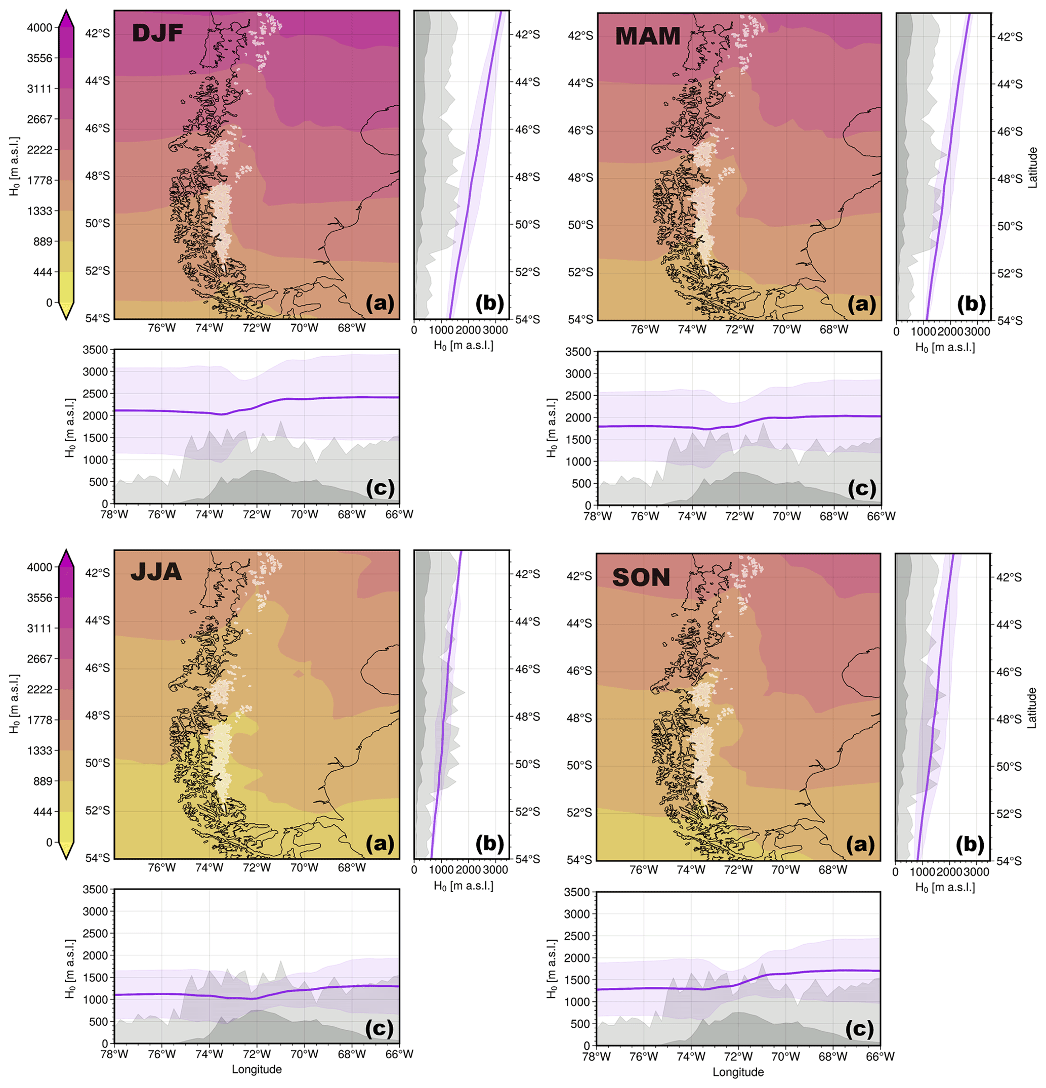
Figure 7 Spatial distribution of the seasonal averages of H₀ (a). The lighter areas depict a lower height of H₀, while the red areas indicate higher values. The white contours delineate the extent of ice coverage in the region. Each seasonal distribution is accompanied by a latitudinal profile (b) and a longitudinal profile (c), showcasing the spatially averaged H₀ values. The purple-shaded area in these profiles represents the respective interquartile range for each profile (IQR_m,z). The grey contours illustrate topographic profiles corresponding to the 2.5th percentile (dark grey) and 97.5th percentile (light grey).

In autumn, the decrease in the freezing-level height is evident. During this season, the average isotherm drops to 1891 m a.s.l., while the variations in the latitudinal and longitudinal profiles are smaller than in summer, ranging from 1066–2848 and 841–2858 m a.s.l., respectively.

During the winter months, the lowest values are recorded. In this season the mean value was estimated at 1169 m a.s.l., and the spatial variability range is narrower, spanning 591–1799 (latitudinal range) and 447–1931 m a.s.l. (longitudinal range). These conditions allow the 0 °C isotherm height to intercept a significant portion of the higher and even lower terrain, especially around 73.5° W, as indicated by the longitudinal profile.

In spring, an average H₀ at 1477 m a.s.l. was estimated, being the second-lowest freezing-level value after winter. For these months, an increase in the amplitude of the latitudinal and longitudinal isotherm ranges was already evident, with values ranging from 701–2449 and 596–2440 m a.s.l., respectively. However, despite the greater variability observed in the freezing level, the interception of the isotherm field with a significant portion of the higher terrain persists, particularly on the western slope of the Andes.

It is worth highlighting that the seasonal variations in Patagonia maintain and modulate the characteristic latitudinal and longitudinal gradient of the region, causing the estimated 0 °C isotherm to fluctuate in a way that preserves its general spatial structure.

3.4 Trends of H₀

From an annual perspective, our findings revealed positive and statistically significant trends in the freezing level across the region (${\stackrel{\mathrm{‾}}{T}}_{\mathrm{0}}^{\mathrm{Annual}}=$ 23.8 m per decade, Table S5). Spatially, the highest average annual trend, reaching up to 36.5 m per decade, was observed in northwestern Patagonia, while the lowest, at 8.8 m per decade, was reported in the southernmost part of the region (Fig. S2).

A seasonal analysis reveals that the summer season has the most pronounced trends compared to other seasons (${\stackrel{\mathrm{‾}}{T}}_{\mathrm{0}}^{\mathrm{DJF}}=$ 40 m per decade). This trend is particularly notable in the northwestern region of Patagonia, reaching a maximum of 60.7 m per decade (Fig. 8, DJF) and a minimum of 18.1 m per decade.

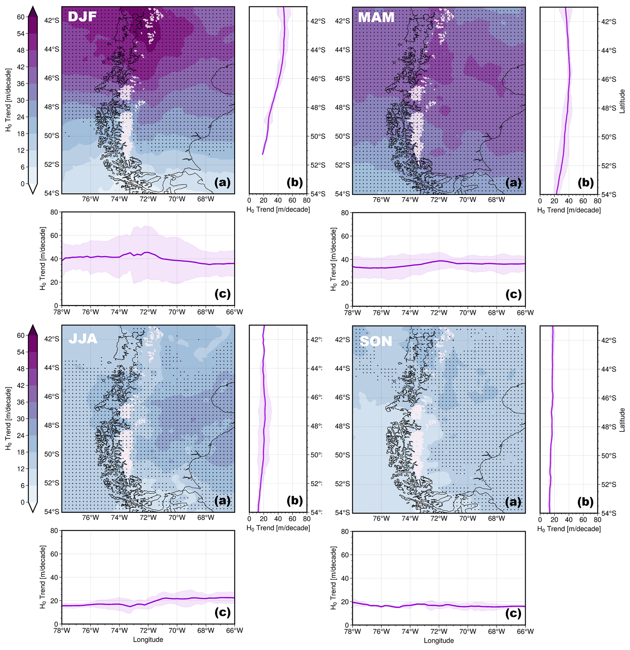
Figure 8 Spatial distribution of the 0 °C isotherm trends (T₀) across the seasons. The lighter areas depict a lower height of the trends, while the purple areas indicate higher values. The white contours delineate the extent of ice coverage in the region. Each distribution is accompanied by a latitudinal profile (b) and a longitudinal profile (c), showcasing the spatially averaged H₀ trend values. The purple-shaded area in these profiles represents the respective interquartile range for each profile (IQR_m,z). The black circles denote statistically significant trends at a p value < 0.05.

The trends diminish during autumn (${\stackrel{\mathrm{‾}}{T}}_{\mathrm{0}}^{\mathrm{MAM}}=$36 m per decade), and there is a shift in the spatial distribution of these trends (Fig. 8, MAM). In contrast to the summers, the field becomes more homogeneous, with high trend values dispersed in the northwest and the central area, where a maximum of 45.5 m per decade is observed. Conversely, the minimum trend during this season is 17.5 m per decade.

In winter (Fig. 8, JJA), the trend continues to decrease, reaching the second-lowest seasonal value (${\stackrel{\mathrm{‾}}{T}}_{\mathrm{0}}^{\mathrm{JJA}}=$19 m per decade). The highest and lowest values during this season are 30.1 and 8.4 m per decade, respectively.

Spring shows the lowest trends (${\stackrel{\mathrm{‾}}{T}}_{\mathrm{0}}^{\mathrm{SON}}=$ 16 m per decade). The spatial distribution of trend values is homogeneous; therefore, the latitudinal and longitudinal profiles are almost steady (Fig. 8, SON). Considering the significant values, it is evident that this seasonal distribution is the most homogeneous, except for the northwestern and central Patagonia regions, where slight increases in the trend are observed, reaching a maximum value of 22.4 m per decade. The minimum estimated trend is located over Tierra del Fuego, with a value of 10.5 m per decade.

3.5 Large-scale control over H₀ variability

To investigate the influence of other large-scale processes on the 0 °C isotherm in Patagonia, we conducted an EOF analysis with annual anomalies of the 0 °C isotherm (Sect. 2.3). Following the methodology of North et al. (1982), we selected the first three principal modes (Fig. S4), which together represent 96 % of the interannual variability (Fig. 9). The first mode of the EOF represents approximately 84 % of the interannual variance of the 0 °C isotherm height in the region. Its spatial distribution represents a monopole that concentrates in the northwestern region of Patagonia, coinciding with the spatial distribution of the trends recorded in the area (Figs. 8a and S2) and covering glacial areas and the northwestern coast, between approximately 42–46° S. Figure 9b indicates the temporal component of the first mode, highlighting the high and significant correlation (r=0.85) between PC1 (red) and the average annual anomalies in the region (grey). In contrast, the second and third components show no significant relationship with H₀ anomalies ($\left|r\right|<\mathrm{0.1}$). Figure 9b also indicates that the highest trends in annual anomalies of the 0 °C isotherm (grey contours, 0.149 and 0.144 m per decade) were recorded in the 1970s and 2010s. According to our results, the most recent decade has presented the highest positive anomalies (Fig. 9b), which coincide with a persistent positive phase of SAM since 2010 (Fig. S4d; Fogt and Marshall, 2020). The correlations obtained between PC1 and SAM, R1-T850, and R2-SST (Fig. 10) indicate significant and positive correlations (r>0.56).

Figure 9 First three leading modes of variability extracted through an empirical orthogonal function (EOF) analysis conducted on Patagonia's annual freezing-level field spanning 1959 to 2021. (a, c, e) The resulting patterns are presented as regression maps, illustrating the relationship between the leading principal component (PC) time series and the spatial distribution of the time-varying height anomalies. Additionally, the temporal pattern is illustrated by the first principal component (red line), scaled to unit variance (divided by the square root of its eigenvalue), while the grey line portrays the standardized anomalies of the spatial average of the annual freezing-level field across Patagonia (b, d, f). In panel (b), the grey box indicates the Pearson correlation between these two patterns, and the grey contour area represents the periods with the highest anomaly trend with their respective values. We continue the analysis for the second and third modes of variability (c–d and e–f, respectively). However, these modes show low correlation values with the freezing-level anomalies, and thus the focus is shifted away from freezing-level anomalies in these cases. The white (a) and grey (c, e) contours delineate the extent of ice coverage in the region.

The second mode explains 8 % of the variability of H₀ and is characterized by a latitudinal gradient, showing positive values in the northeastern region and negative values in the southwest. Significant correlations are found with the Z300 Drake ($r=-\mathrm{0.68}$), T850 Drake ($r=-\mathrm{0.51}$), and R3-U850 (r=0.53) indices. On the other hand, the third mode represents around 4 % of the variability of H₀. It displays a longitudinal gradient with positive values in the northwestern side and negative values in the southeast. Significant correlation between pairs of indices and this mode only was found with Z300 Drake (r=0.39) and R3-U850 ($r=-\mathrm{0.41}$). Additionally, the correlation obtained from indices such as the El Niño–Southern Oscillation (ENSO 1+2 and 3.4) with the leading modes showed low and non-statistically significant correlations ($\left|r\right|<\mathrm{0.2}$).

Figure 10 Correlation matrix between the standardized indices, H₀ anomalies, and principal components obtained from the analysis. Only statistically significant values (p value < 0.05) are shown.

4 Discussion

1. The 0 °C isotherm and ERA5 reanalysis.

   The validation process indicated a high similarity between the 0 °C isotherm height values obtained from radiosondes and the reanalysis data. The greatest uncertainty occurred in Río Gallegos; however, the validation parameters (i.e. correlation, bias, standard deviation, and RMSE) are acceptable. This is especially noteworthy considering that radiosonde data in Río Gallegos encompass a shorter period (n=2194, 1967–1977) compared to other launch sites, representing approximately 10 % of the data compared to Puerto Montt, which has the highest number of records (n=21 251).

   However, we observed an underestimation of the 0 °C isotherm height calculated from reanalysis data when compared with the 0° isotherm derived from radiosonde stations. Overall underestimation of the 0 °C isotherm height obtained from the ERA5 reanalysis has previously been documented by Schauwecker et al. (2022). They estimated an underestimation (overestimation) by the reanalysis at low- (high-)elevation sites, but reasons were not discussed. In our case, all radiosonde points are located near sea level with heights not exceeding 84 m a.s.l.; therefore the underestimation is consistent with findings by Schauwecker et al. (2022). To explore this feature, we conducted seasonal validation and comparison (Table S2). During summer (December to February), the underestimation of the reanalysis was lower compared to winter (June–August) at stations on the west side (Puerto Montt and Punta Arenas). Conversely, at stations on the east side (Comodoro Rivadavia and Río Gallegos), the underestimation decreased (increased) during winter (summer) months. In our study area, we hypothesized that the underestimation of the reanalysis data may be linked to the environmental conditions of the radiosonde launch location points. For instance, topographic conditions are similar (i.e. low elevation, nearby to the sea, and more than 30 km away from larger topographic barriers such as the AA). However, further research and more data (stations or radiosondes) are necessary to better understand the underestimation of the reanalysis and its regional differences in Patagonia.

2. The 0 °C isotherm in Patagonia.

   It is well documented that the orographic influence of the Andes in Patagonia generates meteorological gradients (e.g. precipitation, temperatures, cloudiness, radiation) between the western and eastern sectors (i.e. Garreaud et al., 2009; Garreaud et al., 2013). The 0 °C isotherm is not an exception, showing clear longitudinal differences, with warmer conditions in the eastern sector compared to the western sector. This has implications for the type of precipitation (liquid or solid) and its spatial difference for a given latitude, as has been reported previously (i.e. Viale et al., 2019). However, our results indicate that, south of 52° S, the difference between the western and eastern zones decreases due to the topographic descent of the AA. This is consistent with the analysis of the annual cycle indicated by Garreaud et al. (2009), which shows that temperature differences between both sectors decrease at this latitude (see Fig. S5).

   Finally, it is worth noting that our trend results are comparable with other values reported in the area by Aguayo et al. (2019), who estimated a seasonal trend (DJF, 1970–2018) of 50 m per decade in the Puelo River basin (Fig. 8a and Table S1).

3. Large-scale drivers.

   Similar to the analysis conducted with the SAM (Figs. 10 and S6), a spatial and temporal correlation analysis was also performed to investigate possible links with other large-scale indices such as El Niño–Southern Oscillation (ENSO 1+2 and 3.4) and Pacific Decadal Oscillation (PDO) (analysis not shown). However, no significant correlations were found to suggest any relationship between these indices and the elevation of the 0 °C isotherm in the region. On the other hand, the strong correlation between PC1 and annual anomalies of the 0 °C isotherm, SAM, R1-T850, and R2-SST could provide indications of an interaction mechanism involving all variables. It has been documented by Garreaud et al. (2009) that during the positive phase of SAM, adiabatic warming occurs due to subsidence at the north of the polar jet, resulting in drier conditions in northern Patagonia, while southern Patagonia experiences wetter-than-normal conditions. Opposite conditions occur during the negative phase of SAM. The relationship between the positive phase of SAM and the warming of sea surface temperature in the western Pacific has also been documented (Thomas et al., 2017). Given the high correlation between SAM and SST, it is unknown whether it is possible to explain a mechanism that decouples processes between these variables to better understand their involvement in 0 °C isotherm variations. However, the positive feedback mechanism between SAM (higher temperatures in northern Patagonia) and SST (increased Pacific temperature) could be contributing to the increase in the 0 °C isotherm elevation in northwestern Patagonia. Our results are consistent with projections in the area, which point to drier conditions in northwestern Patagonia under high-greenhouse-gas-emissions scenarios by the end of the century (Collins et al., 2013). Regarding the southern zone and EOF1, the highest spatial correlations obtained involve sea surface temperature (R2-SST) and temperature over the Drake Passage (R1-T850), particularly in the southwestern zone.

   Given the correlations of the second principal component (Fig. 10), we believe this mode may be related to clear-sky conditions that favour a near-surface inversion layer. For example, before events with positive values of R1-Z300 and R1-T850 (conditions of a ridge passage over the Drake Passage), the values of H₀ will decrease (lower freezing level). In terms of PC2 and R3-U850 (r=0.53), the zonal wind could contribute to this process; westward zonal winds (u>0) force the passage of these systems. According to the spatial configuration of this mode, the described mechanism would be limited to the southwestern zone of the region.

   Finally, the third mode (EOF3) presents significant and positive correlations with R1-Z300 and negative correlations with R3-U850. We associated these correlations with the passage of a migratory high in the region, which generates favourable conditions for the generation of Puelche winds characterized by negative zonal winds ($u<-\mathrm{4}$ m s⁻¹; Montecinos et al., 2017), descending and compressing adiabatically in the leeward side, injecting high temperatures into the western zone of the AA, especially the southwestern zone. Indeed, this synoptic configuration is associated with the increase in heatwave events in the area since 1980 (Gonzalez-Reyes et al., 2023).

   Additionally, Fig. 9b indicates the temporal variation in the principal component along with the 0 °C isotherm anomalies. In the last decade, a period of persistent positive anomalies and an increasing trend in the 0 °C isotherm (0.144 m per decade) can be observed. Further, a decrease in precipitation in northwestern Patagonia between 2010–2016 has been reported, with an extreme drought period during the summer of 2016 (Garreaud, 2018). This period coincides with a positive trend in the 0 °C isotherm in the last decade, making it an area of special attention and monitoring.

4. Impact on Patagonian glaciers.

   Patagonia is characterized by extensive icefields: the Southern Patagonia Icefield, Northern Patagonia Icefield, and Cordillera Darwin. As found by Caro et al. (2021), glacier surface mass balance depends on many factors, such as precipitation, temperature, slope, orientation, and others. Because of this, quantifying glacier variations in a region where the 0 °C isotherm is rising is complex. Estimated rise in the 0 °C isotherm impacts the surface mass balance, especially surface mass balances situated in the northwestern region. The consequences of freezing-level rise will vary depending on the sensitivity of each glacier's mass balance and its specific topographic characteristics, such as the area of accumulation versus the area of ablation of a specific glacier. Sensitivity analysis by Caro et al. (2021) determined that glaciers are primarily sensitive to temperature changes in Patagonia. However, if we also consider a future scenario with a higher concentration of greenhouse gases and radiative forcing (i.e. under the SSP5-8.5 scenario), we hypothesize a rise in the height of the 0 °C isotherm, leading to a decrease in solid precipitation in the area. This would affect water resources due to the reduction in glacier volumes (lower accumulation) and increase the region's vulnerability to natural hazards such as floods and glacier lake outburst floods (GLOFs) (Dussaillant et al., 2010; Piret et al., 2022).

5 Conclusions

Through vertical temperature profiles, values of the 0 °C isotherm height were obtained using radiosonde observations and ERA5 data from 1959–2021 in Patagonia. The reanalysis data showed robust estimation of daily observed values and facilitated the derivation of spatial averages that describe the state of the 0 °C isotherm within the study area. The relationship between the main atmospheric modes of the 0 °C isotherm interannual variability and time series of different climatic indices was investigated employing correlations. This approach aimed to discern the large-scale climatic processes governing interannual variations in the freezing level in Patagonia. Some significant findings are as follows.

The histogram of spatial averages indicates a right-skewed distribution in H₀ in Patagonia. Specifically, in the western Andes zone (western section of 72° W), the annual average (median) altitude is approximately 1568 (1347) m a.s.l. In contrast, the eastern Andes zone exhibits a mean (median) of 1818 (1709) m a.s.l. The annual values of the 0 °C isotherm height in Patagonia range from 2658 m a.s.l. in the north to 913 m a.s.l. in the south. The spatio-temporal annual average (median) of the field is 1691 (1519) m a.s.l.

Seasonal variations indicate that the 0 °C isotherm's amplitude spans 3346 (summer) to 575 m a.s.l. (winter).

A pronounced longitudinal gradient is noteworthy, intensifying around 72° W, associated with a drier atmosphere influenced by the orographic lee-side effect of the Andes. The latitudinal gradient behaves as expected (typical temperature gradient of the transition to extratropics), gradually decreasing southward with latitude. This spatial configuration persists throughout the months, with the distinction that higher freezing-level heights are recorded during summers. In this season, the longitudinal average is estimated not to intersect with the highest topography (95th percentile of topography). Contrasting conditions prevail during winter, where the lowest freezing-level values are observed, and on average, the longitudinal profile of the 0 °C isotherm intersects the highest (P95) and lowest (P5) topography around 72° W, essentially aligning with the Andes Mountain range. Autumn and spring months are transitional periods between the more pronounced summer and winter seasons.

Throughout the years, the 0 °C isotherm level in Patagonia exhibited a consistent variation with temperature changes, marked by an increase in temperature within the whole region. This temperature shift translates into an annual spatial average increase in the freezing-level height, ranging from 36.5 to 8.8 m per decade. Seasonally, the highest trends were observed during summers, specifically in northwestern Patagonia, around the Andes, indicating an average increase in freezing heights of 61 m per decade. On average, winter trends are lower but remain positive, reaching average values of 8.4 m per decade in areas surrounding the Andes.

The primary mode of variability accounts for about 84 % of the variance in the H₀ field. Spatially, this mode shows predominantly positive values across the entire area, notably in central and northeastern Patagonia, which aligns with the locations of the highest estimated trends. Temporally, this mode shares interannual variability with Patagonia's average field of 0 °C isotherm anomalies. Thus, years with positive phases of the first principal component (PC1) are associated with positive anomalies in freezing-level height. Similarly, this mode shows a positive and significant correlation with SAM, temperature at 850 hPa in the Drake Passage, and sea surface temperature in the Pacific Ocean near the western coasts of Patagonia. The second and third modes explain 8 % and 4.4 % of the data variance, respectively. Their spatial configuration indicates both a latitudinal and a longitudinal dipole in the study area. The second mode exhibited significant correlations with R1-Z300 (+), R1-T850 (−), and R3-U850 (−), while the third mode correlated significantly with R1-300 (+) and R3-U850 (−).