A simple model linking radiative–convective instability, convective aggregation and large-scale dynamics

A simple model is presented which is designed to analyse the relation between the phenomenon of convective aggregation at small scales and larger-scale variability that results from coupling between dynamics and moisture in the tropical atmosphere. The model is based on single-layer dynamical equations coupled to a moisture equation to represent the dynamical effects of latent heating and radiative heating. The moisture variable q evolves through the effect of horizontal convergence, nonlinear horizontal advection and diffusion. Following previous work, the coupling between moisture and dynamics is included in such a way that a horizontally homogeneous state may be unstable to inhomogeneous disturbances, and, as a result, localised regions evolve towards either dry or moist states, with divergence or convergence respectively in the horizontal flow. The time evolution of the spatial structure of the dry and moist regions is investigated using a combination of theory and numerical simulation. One aspect of the evolution is a spatial coarsening that, if moist regions and dry regions are interpreted as convecting and non-convecting respectively, represents a form of convective aggregation. When the weak temperature gradient (WTG) approximation (i.e. a local balance between heating and convergence) applies, and horizontal advection is neglected, the system reduces to a nonlinear reaction–diffusion equation for q, and the coarsening is a well-known aspect of such systems. When nonlinear advection of moisture is included, the large-scale flow that arises from the spatial pattern of divergence and convergence leads to a distinctly different coarsening process. When thermal and frictional damping and f-plane rotation are included in the dynamics, there is a dynamical length scale L_dyn that sets an upper limit for the spatial coarsening of the moist and dry regions. The f-plane results provide a basis for interpreting the behaviour of the system on an equatorial β plane, where the dynamics implies a displacement in the zonal direction of the divergence relative to q and hence to coherent equatorially confined zonally propagating disturbances, comprising separate moist and dry regions. In many cases the propagation speed and direction depend on the equatorial wave response to the moist heating, with the relative strength of the Rossby wave response to the Kelvin wave response determining whether the propagation is eastward or westward. Within this model, the key overall properties of the propagating disturbances, the spatial scale and the phase speed, depend on nonlinearity in the coupling between moisture and dynamics, and any linear theory for such disturbances therefore has limited usefulness. The model described here, in which the moisture and dynamical fields vary in two spatial dimensions and important aspects of nonlinearity are captured, provides an intermediate model between theoretical models based on linearisation and one spatial dimension and general circulation models (GCMs) or convection-resolving models.

1 Introduction

Much theoretical and modelling work over the past few decades has focused on the coupling between dynamics and moisture in the tropical atmosphere, which has been argued should be taken into account at leading order to explain many tropical phenomena. Two topics that continue to attract significant attention are on the one hand convective aggregation, identified as a behaviour in numerical simulations in convection-representing models, and on the other hand the Madden–Julian Oscillation (hereafter MJO), identified in observations as a dominant mode of intraseasonal variability of the real tropical atmosphere. Convective aggregation (e.g. Wing et al., 2017; Muller et al., 2022) has been identified as a pattern of behaviour of a hypothetical tropical atmosphere in which there is no imposed spatial inhomogeneity but which exhibits spontaneous organisation of the circulation and convection into regions of two types, one type with active convection and large-scale ascent and the other with convection suppressed by large-scale subsidence. The relevance of convective aggregation to the behaviour of the real atmosphere remains a topic of debate, but the study of aggregation in convection-representing numerical models (hereafter CRMs) has provided a great deal of insight into the physics of the tropical atmosphere, particularly the interactions between convecting and non-convecting regions, and the way in which this physics is represented in models. It has been suggested that the same physics that is responsible for convective aggregation in numerical simulations is also part of the mechanism for the MJO (Bretherton et al., 2005; Arnold and Randall, 2015). Investigating this possibility in numerical simulations has been challenging because the numerical resolution for CRM simulations is a few kilometres or less, and the spatial structure of the MJO has scales of several thousand kilometres. A small number of papers (e.g. Arnold and Randall, 2015; Khairoutdinov and Emanuel, 2018) have described simulations that bridge this gap and have given insight into the relation between convective aggregation and the spontaneous generation of large-scale MJO-like disturbances. Other papers (e.g. Carstens and Wing, 2022, 2023) have used CRM simulations to explore more generally the relation between convective aggregation and larger-scale dynamics. Since such simulations are at the very edge of current computational capacity and the scope for thorough examination of parameter space is limited, it is desirable to find a simpler theoretical and modelling framework within which the link between processes such as aggregation on the mesoscale and larger-scale organisation of dynamics can be investigated further. The focus of this paper is the formulation and study of a simple model for such a purpose.

Several different physical processes have been proposed as being important for aggregation, often supported by the results of mechanism-denial experiments in CRMs in which the effects of particular processes have been altered or omitted altogether. As emphasised by Muller et al. (2022), there remains considerable uncertainty over which of these various descriptions of the aggregation process is most relevant to convective aggregation and, within each of them, the relative importance of different physical mechanisms. Examples of suggested mechanisms include the spatio-temporal propagation of triggering of convection through different effects, either through the formation and propagation of cold pools (e.g. Hirt et al., 2020) or through the propagation of gravity waves within the boundary layer (Yang, 2021). The study described in this paper is prompted in particular by the proposal that aggregation occurs via an instability of a spatially homogeneous radiative–convective equilibrium state resulting from feedbacks between moisture and radiation (Raymond, 2000; Emanuel et al., 2014), primarily in the free troposphere, though the boundary layer (Yang, 2018) may play a crucial role in the dynamics of these feedbacks. Instability, generally described as radiative instability or radiative–convective instability, may result if these feedbacks can overcome the dynamical stability of the convecting atmosphere. The competition between these processes is typically represented by the gross moist stability (GMS; e.g. Raymond et al., 2009), though changes in convective moisture and heat transport should be properly taken into account (Beucler et al., 2018). The growing instability is expected to ultimately saturate at finite amplitude with the result that locally the system tends towards a moist or a dry state. Such behaviour has been demonstrated using single-column radiation–convection calculations using various standard radiative and convective parametrisations and adopting the weak temperature gradient (WTG) assumption where the environmental temperature is specified, and the vertical mass flux is allowed to be non-zero (Sobel et al., 2007; Emanuel et al., 2014). Under suitable conditions the radiative–convective equilibrium (RCE) state is unstable, and the system evolves towards a moist state or a dry state, depending on the imposed initial perturbation.

A more generic and fundamental approach to the study of convective aggregation, starting with instability as the initial mechanism for the growth of moisture inhomogeneities on the homogeneous state but then seeking a description of the spatial evolution of the resulting moist and dry regions, has been undertaken by Craig and Mack (2013) and Windmiller and Craig (2019) (hereafter CMWC). The model system considered in this work is an evolution equation for a time-evolving two-dimensional moisture concentration field q, incorporating a source–sink term that is a nonlinear function of q, say G(q), with three zeros, each corresponding to possible steady states. The form of the function G(q) is such that the large-q (moist) and small-q (dry) states are stable, and the intermediate-q state is unstable. Transport of moisture is assumed to be diffusive. This system is equivalent to a reaction–diffusion equation with bistable reaction, sometimes known as the Allen–Cahn equation, which has been extensively studied using theoretical and numerical approaches. Such systems exhibit coarsening where, after the initial separation into high-q and low-q regions, typically on small scales, the scale of these regions increases monotonically with time, until it is constrained by the large-scale geometry imposed on the system. This is presented by CMWC as a mechanism for aggregation. The two essential components required for this mechanism to operate are the q dependence, and hence the bistable nature of the source–sink term, which CMWC argue results from the dependence of subsidence drying and convective moistening on free-tropospheric moisture, and the diffusive transport. Windmiller and Craig (2019) argue that diffusive transport can be justified on the basis of a simple model in which a stochastic convective cloud moistens the environment of a moist region, and they provide an estimate for the resulting diffusivity as 4×10² m² s⁻¹. A larger value of the diffusivity, 10⁵ m² s⁻¹, is used in Craig and Mack (2013) and is envisaged as being based on the typical horizontal velocity and length scales of convective systems. The latter justifies this as an eddy diffusivity based on the typical horizontal velocity and length scales of convective motions. The appropriate value of the diffusivity therefore depends significantly on what the diffusivity is intended to represent. This reaction–diffusion model for aggregation is interesting, and it is discussed further in the Muller et al. (2022) review, but, since large-scale dynamics is omitted from the model, it cannot be used to investigate the link between convective aggregation and large-scale dynamics.

The model presented in this paper combines aspects of the CMWC model with a simple description of large-scale dynamics. The structure of this paper is as follows. In Sect. 2 we define the mathematical model to be studied, following previous approaches that use the shallow-water equations augmented by a prognostic equation for moisture, with the moisture coupling to the shallow-water dynamics. We then set out the behaviour expected of the model on the basis of previous work together with various scaling arguments, explaining the relation to CMWC. In Sect. 3 we present results from numerical simulations of the system on a doubly periodic domain. In particular, we verify that aggregation occurs and that the mechanism for aggregation can be dominated by horizonal diffusion of moisture or by horizontal advection of moisture, depending on the external parameters defining the system. In Sect. 4 we then show that rotation, thermal damping and frictional damping can each, or in combination, lead to a finite upper limit on the aggregation scale. This is with both theoretical arguments and results from numerical simulations on a doubly periodic f plane (including the zero-rotation case f=0). In Sect. 5 we exploit the f-plane results derived previously to consider the system on an equatorial β plane and show that the process of aggregation is then confined to a low-latitude region with the result of aggregation being the formation of coherently propagating disturbances. The scale and propagation speed of these disturbances depend on the external parameters, in particular, in some regimes, the relative strength of the equatorial Kelvin and Rossby wave responses to the moist heating. In Sect. 6 we discuss the results and present overall conclusions.

Whilst we have mentioned above the MJO as a key motivation for further investigation of tropical dynamics, the model as presented in this paper does not reach the stage of direct relevance to the MJO or other aspects of tropical intraseasonal variability. That requires further development to be reported in a future paper. We simply note that the model presented here can be regarded as belonging to the class of “moisture-mode” models studied by Sugiyama (2009a), Sugiyama (2009b), Sobel and Maloney (2012), Sobel and Maloney (2013), Adames and Kim (2016), and others but that this class is one of several different classes of theoretical models for the MJO that continue to be studied, as recently reviewed by Jiang et al. (2020) and Zhang et al. (2020).

2 Model system to be studied

2.1 Model equations

The model to be studied in the remainder of the paper follows much previous work in being based on the dynamical equations for a rotating shallow-water system, describing the evolution of horizontal velocity u and free-surface displacement h, augmented by a moisture variable q, which is transported by the horizontal velocity. Such single-layer equations can be derived from primitive equations and the corresponding moisture equation for a stratified three-dimensional atmosphere following the systematic procedure set out by Neelin and Zeng (2000) based on a vertical-mode decomposition for dynamical quantities and for moisture. Specific further simplifications, following e.g. Sugiyama (2009b), over the set of equations presented by Neelin and Zeng (2000) (their 5.1–5.4) are that the barotropic flow and the nonlinear terms in the dynamical equations are neglected.

To emphasise the overall structure of the equations, rather than the details determined by the modal decomposition, we simply write the dynamical equations in the standard form for the motion, linearised about a state of rest, of a shallow layer of fluid with undisturbed depth H:

$$\begin{array}{}\text{(1)}& {\mathit{u}}_t=-f\mathit{k}\times \mathit{u}-g\mathrm{\nabla }h-\mathit{\alpha }\mathit{u}\end{array}$$

and

$$\begin{array}{}\text{(2)}& h_t+H\mathrm{\nabla }\cdot \mathit{u}=F_h\left(q\right)-\mathit{\lambda }h,\end{array}$$

where g is the gravitational acceleration, and f is the Coriolis parameter, which will be taken to be either constant f=f₀, corresponding to the f plane, or linearly dependent on the y coordinate, f=βy, corresponding to the equatorial β plane. k is the unit vector in the vertical. α is a linear friction coefficient and λ a thermal damping rate. The corresponding equation for the moisture variable q is

$$\begin{array}{}\text{(3)}& q_t+Q\mathrm{\nabla }\cdot \mathit{u}+\mathrm{\nabla }\cdot \left(q\mathit{u}\right)-\mathit{\kappa }{\mathrm{\nabla }}^{\mathrm{2}}q=F_q\left(q\right),\end{array}$$

including both horizontal advective transport and horizonal diffusive transport, the latter with diffusivity κ, assumed to be constant. In these equations, u is to be interpreted as representing the lower-tropospheric horizontal velocity field, and the displacement h is a surrogate for mid-troposphere temperature, with temperature increasing as h decreases. Given typical choices for the vertical basis function for moisture (Zeng et al., 2000), q is to be interpreted as the lower-tropospheric moisture concentration. The values of the constants H, α and λ could be chosen to match the values implied by the modal decomposition and by corresponding approximations to detailed parametrisations of physical processes, as set out in Neelin and Zeng (2000) and Sugiyama (2009b), but for the purposes of the work reported here, we simply chose values typical of those chosen in previous work on simple modelling of the tropical atmosphere.

The term F_h(q), included on the right-hand side of Eq. (2), represents a moisture-dependent cooling term (cooling because of the relation between h and temperature), potentially including both latent heating and radiative heating. If cooling decreases with moisture, as is physically plausible, F_h(q) will then be a decreasing function of q. Correspondingly, the term F_q(q) on the right-hand side of Eq. (3) represents the combined effects of evaporation and precipitation. The part of F_q(q) representing precipitation (note that F_q(q) is a negative contribution to precipitation) is also expected, on the basis of the observed correlation between precipitation and moisture in the free troposphere (e.g. Holloway and Neelin, 2009), to be a decreasing function of q. Q is a suitably chosen constant so that q is the perturbation away from a background state where the “total” moisture variable is Q, and it is convenient to choose Q such that F_q(0)=0, i.e. such that in the background state there is a balance between evaporation and precipitation. Previous papers developing and exploiting the simplified set of equations, Eqs. (1), (2) and (3), such as Neelin and Zeng (2000), Zeng et al. (2000), and Sugiyama (2009b), have given detailed arguments for how these moisture-dependent terms F_h(q) and F_q(q) might be constructed from specific parametrisation schemes for radiation and convection. Here we choose simplified ad hoc forms for these terms. A specific simplification made is that both terms F_q and F_h are assumed to be independent of h; i.e. the evaporation–precipitation and the moisture-dependent part are assumed to be independent of temperature. Whilst temperature (or h) dependence of these moisture coupling terms is neglected in several previous papers (Adames and Kim, 2016; Sobel and Maloney, 2012, 2013), it is included by Sugiyama (2009a, b). We briefly examine the effect of such dependence, with results reported in Appendix E and further comments in Sect. 6.

Within the constraints of the very simple model specified above, we can identify the possibility of choosing H and Q such that $h=q=\mathrm{0}$ corresponds to a spatially homogeneous radiative–convective equilibrium (RCE) state with u=0 and F_h and F_q satisfying the conditions $F_h\left(\mathrm{0}\right)=F_q\left(\mathrm{0}\right)=\mathrm{0}$. We can restrict the forms of F_h(q) and F_q(q) to those for which the system is stable to spatially homogeneous perturbations, which holds if $\partial F_q/\partial q<\mathrm{0}$, with the partial derivative being evaluated at q=0. A key question is then whether, within this restriction, the radiative–convective equilibrium (RCE) state is unstable to spatially inhomogeneous disturbances. We demonstrate below that such instability is possible for relatively simple choices of the functions F_h(q) and F_q(q), and we interpret this instability as the analogue, within this simple model, of “radiative–convective instability” that has previously been discussed in several papers and demonstrated in suitable single-column radiation–convection calculations (e.g. Sobel et al., 2007; Emanuel et al., 2014).

The key dimensional quantities that define the above system include g and H, which determine the dry gravity wave speed $c=\sqrt{gH}$; the horizonal diffusivity κ; the Coriolis parameter f; the thermal and frictional damping rates, λ and α respectively; a typical background value of moisture, say Q; and μ, an inverse timescale for the moist processes represented by F_h and F_q. It is convenient to take the dimensions of the moisture Q to be the same as those of the thickness H, and indeed this corresponds to a simple re-scaling of the parameters in F_h. To assess the importance of the advective term in Eq. (3), an additional dimensional quantity is needed which sets the magnitude of the spatially inhomogeneous part of the moisture field and, hence, via the leading-order balances operating in Eq. (2) and (3), the magnitude of the corresponding horizontal flow. These magnitudes are set by the nonlinear dependence of F_q and F_h on q, but it is convenient to choose the magnitude, say D, of the divergence ∇⋅u , as the relevant dimensional quantity. The reason for this becomes clear from the discussion in Sect. 2.2 below.

The fact that the magnitude of the advective nonlinearity arising in Eqs. (1), (2) and (3), as written above, depends on the choice of F_h(q) and F_q(q) potentially complicates interpretation of the behaviour of the system, and there are advantages to allowing the advective nonlinearity to be varied independently of this choice. We therefore introduce the parameter ϵ into Eq. (3) to give

$$\begin{array}{}\text{(4)}& q_t+Q\mathrm{\nabla }\cdot \mathit{u}+\mathit{ϵ}\mathrm{\nabla }\cdot \left(\mathit{u}q\right)-\mathit{\kappa }{\mathrm{\nabla }}^{\mathrm{2}}q=F_q\left(q\right).\end{array}$$

The linear instability analysis of the RCE state, for example, takes ϵ=0 in the above equation. Note that in the form of the equations considered by Sugiyama (2009b), derived from the Neelin and Zeng (2000) Quasi-equilibrium Tropical Circulation Model (QTCM) equations, there is a distinct constant multiplying the nonlinear advective term. This constant is determined in principle in the derivation of the single-layer equations by the projection of a horizontal moisture advection term that varies in height onto the single basis function used to represent the moisture field, but it can also be conveniently varied as an independent parameter, and ϵ introduced here plays the same role as that parameter. We illustrate the role of advective nonlinearity by comparing ϵ=1 behaviour with ϵ=0 behaviour, but note that, for the reasons just given, ϵ=1 cannot be regarded as the only “correct” choice for including advective nonlinearity.

2.2 WTG and the relation to the CMWC reaction–diffusion system

A standard approach, particularly at low latitudes where f is small, to analysing the system defined by Eqs. (1)–(3) is to make the weak temperature gradient (WTG) approximation (e.g. Sobel et al., 2001). This neglects horizontal variation in h and can be justified provided that the horizontal length scale L satisfies $L/c\ll T_q$, i.e. that the timescale for gravity wave propagation through L is much less than the timescale T_q for moist processes. T_q could either be a timescale μ⁻¹ set by an appropriate combination of F_q and F_h (see below) or be an emergent property of the system. Additionally, when damping and rotation are included, it must be the case that L≪L_dyn, where L_dyn is a dynamical length scale that is typically determined by c together with some combination of f, α and λ. We focus on the zero-damping case in this section and return to the dynamical effects of damping and rotation in Sect. 4.

Whilst under WTG h is constant in space, it may not be constant in time. Taking the spatial average of Eq. (2), the overline notation is used to denote the spatial average. It follows that

$$\begin{array}{}\text{(5)}& {\displaystyle \frac{\mathrm{d}\stackrel{\mathrm{‾}}{h}}{\mathrm{d}t}}=\stackrel{\mathrm{‾}}{F_h\left(q\right)}-\mathit{\lambda }\stackrel{\mathrm{‾}}{h}.\end{array}$$

The spatially varying part of Eq. (2) then has the following form:

$$\begin{array}{}\text{(6)}& H\mathrm{\nabla }\cdot \mathit{u}=F_h\left(q\right)-\stackrel{\mathrm{‾}}{F_h\left(q\right)},\end{array}$$

implying that ∇⋅u, and hence the irrotational part of the velocity field, is determined instantaneously by the moisture field q. Under the assumption $f=\mathit{\alpha }=\mathrm{0}$ in this section, the rotational part of u is constant in time. When provided with this initial rotational part of the flow, assumed to be zero for the purposes of this section, Eq. (4) becomes a self-contained equation for the evolution of the q field with the following form:

$$\begin{array}{}\text{(7)}& \begin{array}{rl}{q}_t& +\mathit{ϵ}\mathrm{\nabla }\cdot \left(\mathit{u}\right[q\left]q\right)-\mathit{\kappa }{\mathrm{\nabla }}^{\mathrm{2}}q\\ & =F_q\left(q\right)-{\displaystyle \frac{Q}{H}}\left(F_h\right(q)-\stackrel{\mathrm{‾}}{F_h\left(q\right)})=G_{hq}(q;\stackrel{\mathrm{‾}}{F_h\left(q\right)}),\end{array}\end{array}$$

where the second equality defines the function G_hq. Note that whilst evaluation of $\stackrel{\mathrm{‾}}{F_h\left(q\right)}$ requires knowledge of the q field, for the purposes of expressing the right-hand side of the equation as a function of q, $\stackrel{\mathrm{‾}}{F_h\left(q\right)}$ is simply a parameter that appears in the definition of that function. The notation u[q] simply expresses the fact that at each instant u is determined completely, but non-locally, by the q field, through Eq. (6).

Neglecting for a moment the advection term ϵu[q]⋅∇q, this may be recognised as a reaction–diffusion equation of the type studied by CMWC. The difference is that whilst the nonlinear “reaction” term on the right-hand side of Eq. (7) was in CMWC's case entirely determined by the q dependence of precipitation and evaporation, in this case the reaction term is a combination of the moisture-driven heating/cooling F_h(q) and the moisture source/sink F_q(q). A further structural difference from the system considered by CMWC is the evolving quantity $\stackrel{\mathrm{‾}}{h}\left(t\right)$. The effect of this is felt by the system through the corresponding $\stackrel{\mathrm{‾}}{F_h\left(q\right)}$ appearing in the definition of the reaction term. The reaction term is therefore not completely specified in advance as a function of q but contains the spatially constant term $\stackrel{\mathrm{‾}}{F_h\left(q\right)}$, which also drives changes in $\stackrel{\mathrm{‾}}{h}$, as specified by Eq. (5). The Craig and Mack (2013) model, on the other hand, imposes an integral constraint on q, equivalent to specified domain-integrated precipitation, and then accommodates this constraint by multiplying G(q) by an unknown function of t, which is determined from the constraint. Again this means that the complete reaction term requires knowledge of the spatial distribution of q.

Simple theory of the reaction–diffusion system with the specified reaction term G(q) is that (i) homogenous steady states are possible with q equal to the constant value q_s, if G(q_s)=0, and (ii) those homogeneous states are stable if $G^{\prime }\left(q_s\right)<\mathrm{0}$ and unstable if $G^{\prime }\left(q_s\right)>\mathrm{0}$. CMWC consider a bistable system with three possible values for q_s, $q_{-}<q_{\mathrm{0}}<q_{+}$ such that $G\left(q_{-}\right)=G\left(q_{\mathrm{0}}\right)=G\left(q_{+}\right)=\mathrm{0}$ and $G\left(q_{-}\right)<\mathrm{0}$, $G^{\prime }\left(q_{\mathrm{0}}\right)>\mathrm{0}$ and $G^{\prime }\left(q_{+}\right)<\mathrm{0}$. G^′(q₀) provides a useful definition of a reaction inverse timescale μ. The generic behaviour for a nonlinear reaction diffusion equation of this type is that locally q tends to one of the stable values, partitioning the domain into two regions, one with $q=q_{+}$ and the other with $q=q_{-}$, separated by interfaces of thickness $(\mathit{\kappa }/\mathit{\mu }{)}^{\mathrm{1}/\mathrm{2}}$. In the absence of rotation and damping, WTG will break down on length scales of order cT_q, so we require $c{T}_q\gg (\mathit{\kappa }/\mathit{\mu }{)}^{\mathrm{1}/\mathrm{2}}$; i.e. the reaction timescale μ⁻¹ is such that κμ≪c². The initial geometry of these two regions is set by the initial conditions. A useful simple solution is a one-dimensional propagating reactive–diffusive wave solution with $q=q_{+}$ on one side of the wave and $q=q_{-}$ on the other. The speed of propagation of the wave, $c_{\mathrm{RD}}\sim (\mathit{\kappa }\mathit{\mu }{)}^{\mathrm{1}/\mathrm{2}}$, is determined by the form of the reaction function G(q). Defining V(q) by $\mathrm{d}V/\mathrm{d}q=G$ so that V(q) has turning points where G(q) has zeros, then if $V\left(q_{+}\right)>V\left(q_{-}\right)$ the region with $q=q_{+}$ propagates into the region with $q=q_{-}$. The corresponding result for the initial value problem, in one or more space dimensions, is that q tends everywhere to q₊. Similarly, if $V\left(q_{+}\right)<V\left(q_{-}\right)$, then q eventually tends everywhere to q₋. Only in the case of $V\left(q_{+}\right)=V\left(q_{-}\right)$, which applies in particular to the Allen–Cahn equation, do both regions $q=q_{+}$ and $q=q_{-}$ persist. Note that V(q) represents the area under the graph of G(q). To be precise, if the choice V(q₀)=0 is made, then V(q₊) is the area under the graph of V(q) in the interval $[q_{\mathrm{0}},q_{+}]$, and V(q₋) is the corresponding (positive) area in the interval $[q_{-},q_{\mathrm{0}}]$.

An important effect in two dimensions is that the reaction–diffusion velocity c_RD becomes a local property of each point on each interface, depending not only on the form of G(q) but also on the curvature of the interface. The reaction velocity c_RD should be replaced by $c_{\mathrm{RD}}+\mathit{\kappa }/R$, where R is the (signed) radius of the curvature of the interface (such that the propagation is towards the interior of the curve). If $\left|c_{\mathrm{RD}}\right|<\mathit{\kappa }/\left|R\right|$, the velocity of the boundary may even change sign. Therefore, c_RD decreases as the curvature of the interface increases (R decreases) (Rubinstein et al., 1989). This tends to smooth out the boundary between moist and dry regions, as small-scale irregularities or indeed small-scale regions will tend to disappear. Larger moist regions can therefore expand, whilst smaller moist regions shrink. This is the standard coarsening behaviour, i.e. the geometric simplification of the geometry between the two regions through an increase in spatial scales, observed in reaction–diffusion systems (Bray et al., 2003).

The inclusion of an integral constraint on q by Craig and Mack (2013) is important because this ensures that even if $V\left(q_{+}\right)\ne V\left(q_{-}\right)$ (with V(q) defined as above), the system does not simply evolve to $q=q_{-}$ or $q=q_{+}$ everywhere. Both values of q persist as coarsening proceeds. Indeed, if this sort of constraint is not applied, then in most cases the reaction–diffusion system with a bistable reaction evolves everywhere towards one of the stable states. Indeed, Windmiller and Craig (2019) do not apply such a constraint and note that at long timescales one or the other of the q₋ or q₊ states occupies an increasingly large fraction of the domain. It is demonstrated below that the same property holds, with both values of q persisting as coarsening proceeds, for the model system being considered in this study, i.e. for a reaction–diffusion system with the reaction term as specified by the right-hand side of Eq. (7).

Following the arguments presented above, the stability of the spatially homogeneous RCE state will be determined by the derivative with respect to q of $G_{hq}(q,\mathrm{0})=F_q\left(q\right)-(Q/H)F_h\left(q\right)$ at q=0, with instability if the derivative is positive, provided that the domain size is large enough that diffusion does not stabilise the system through the action of the κ∇²q term. (This derivative is later identified as proportional to the negative of the gross moist stability; i.e. the RCE state will be unstable if the gross moist stability is negative.) It is assumed that the derivative is indeed positive and furthermore that G_hq(q;0) is bistable in the sense that there are q₊(0) and q₋(0) such that $q_{-}\left(\mathrm{0}\right)<\mathrm{0}<q_{+}\left(\mathrm{0}\right)$, with $G_{hq}\left(q_{-}\right(\mathrm{0});\mathrm{0})=G_{hq}\left(q_{+}\right(\mathrm{0});\mathrm{0})=\mathrm{0}$ and $G_{hq}^{\prime }\left(q_{-}\right(\mathrm{0});\mathrm{0})<-\mathrm{0}$, $G_{hq}^{\prime }\left(q_{+}\right(\mathrm{0});\mathrm{0})<\mathrm{0}$. Note that this property of G_hq(q;0) implies a similar property, with corresponding $q_{-}\left(\stackrel{\mathrm{‾}}{F_h\left(q\right)}\right)$, $q_{\mathrm{0}}\left(\stackrel{\mathrm{‾}}{F_h\left(q\right)}\right)$ and $q_{+}\left(\stackrel{\mathrm{‾}}{F_h\left(q\right)}\right)$, for the more general right-hand side of Eq. (7), $G_{hq}(q;\stackrel{\mathrm{‾}}{F_h\left(q\right)})$, provided that $\left|\stackrel{\mathrm{‾}}{F_h\left(q\right)}\right|$ is not too large. For notational convenience the explicit dependence of e.g. $q_{-}\left(\stackrel{\mathrm{‾}}{F_h\left(q\right)}\right)$ on $\stackrel{\mathrm{‾}}{F_h\left(q\right)}$ is not displayed unless it is essential.

Numerical solutions below show that if G_hq is bistable in the sense defined, then the system indeed evolves towards two values of q and coarsening occurs. However some further insight can be obtained by assuming that after the initial adjustment the region $q=q_{+}$ fills an area A₊, and the region $q=q_{-}$ fills an area A₋. The area of the interfaces between the regions is assumed to be negligible. The configuration is therefore determined by the three unknowns, q₋, q₊ and A₊ (or A₋).

Then the above equations imply

$$\begin{array}{}\text{(8)}& {\displaystyle }{G}_{hq}(q_{+},\stackrel{\mathrm{‾}}{F_h\left(q\right)})=F_q\left(q_{+}\right)-(Q/H)\left(F_h\right(q_{+})-\stackrel{\mathrm{‾}}{F_h\left(q\right)})=\mathrm{0},\text{(9)}& {\displaystyle }{G}_{hq}(q_{-},\stackrel{\mathrm{‾}}{F_h\left(q\right)})=F_q\left(q_{-}\right)-(Q/H)\left(F_h\right(q_{-})-\stackrel{\mathrm{‾}}{F_h\left(q\right)})=\mathrm{0},\text{(10)}& {\displaystyle }(A_{-}+A_{+})\stackrel{\mathrm{‾}}{F_h\left(q\right)}=A_{+}{F}_h\left(q_{+}\right)+A_{-}{F}_h\left(q_{-}\right).\end{array}$$

These determine any two of the three variables q₋, q₊ and A₊ in terms of the third. For the system to be at a steady state an additional constraint, obtained by integrating Eq. (3) over the domain, might seem to be $A_{+}{F}_q\left(q_{+}\right)+A_{-}{F}_q\left(q_{-}\right)=\mathrm{0}$; however this can be deduced from Eqs. (8) and (9) above and provides no extra information. Therefore it has to be accepted that one piece of further information in addition to the above is required for a unique solution. In general these equations determine a state that is quasi-steady rather than exactly steady. After the initial adjustment, when the required extra information will be determined by the initial conditions (which might, for example, set A₊), we expect a further slow time evolution of the three variables and correspondingly of the geometry of the dry and moist regions.

Assume that the overall effect of this slow time evolution can be captured by the classical theory for one-dimensional reactive–diffusive waves, describing the propagation of the thin interfaces between regions of piecewise constant q. This suggests the (slow) time evolution equation

$$\begin{array}{}\text{(11)}& {\displaystyle \frac{\mathrm{d}{A}_{+}}{\mathrm{d}t}}=L_{\mathrm{interface}}{c}_{\mathrm{RD}}(q_{+},q_{-},\stackrel{\mathrm{‾}}{F_h\left(q\right)}),\end{array}$$

where L_interface is the length of the interface between the regions, and c_RD is the reaction diffusion velocity, with the convention that this is positive if the region with $q=q_{+}$ propagates into the region with $q=q_{-}$. L_interface will vary in time but is certainly positive. This equation allows a steady state when $c_{\mathrm{RD}}(q_{+},q_{-},\stackrel{\mathrm{‾}}{F_h\left(q\right)})=\mathrm{0}$.

That such a steady state exists can be deduced by considering the graphs of the relevant functions of q. As noted previously, for a given $\stackrel{\mathrm{‾}}{F_h\left(q\right)}$ the reaction function is $G_{hq}(q,\stackrel{\mathrm{‾}}{F_h\left(q\right)})=F_q\left(q\right)-(Q/H)F_h\left(q\right)+(Q/H)\stackrel{\mathrm{‾}}{F_h\left(q\right)})$. Consider first the graph of $G_{hq}(q,\mathrm{0})=F_q\left(q\right)-(Q/H)F_h\left(q\right)$ as shown by the curve in Fig. 1, which intersects the q axis at q₋(0), q₀(0) and q₊(0). The value of $G_{hq}(q,\stackrel{\mathrm{‾}}{F_h\left(q\right)})$ is represented by the vertical distance between this curve and the horizontal line $-(Q/H)\stackrel{\mathrm{‾}}{F_h\left(q\right)}$, shown in the figure for various values of $\stackrel{\mathrm{‾}}{F_h\left(q\right)}$, varying between C_min<0 and C_max>0. For C outside this range, G_hq(q;C) no longer has three roots. Areas V₊ and V₋ are marked in the figure for a particular value of $\stackrel{\mathrm{‾}}{F_h\left(q\right)}$. The condition $c_{\mathrm{RD}}(q_{+},q_{-},\stackrel{\mathrm{‾}}{F_h\left(q\right)})=\mathrm{0}$ is satisfied if and only if $V_{+}=V_{-}$. It is clear from the figure that there is one value of $\stackrel{\mathrm{‾}}{F_h\left(q\right)}$, say C_s, for which this holds, lying in the range (C_min,C_max). Substituting this value into Eqs. (8)–(10) gives the corresponding values of q₋ and q₊; the dry and moist values of q; and A₊, the fractional area occupied by the moist region.

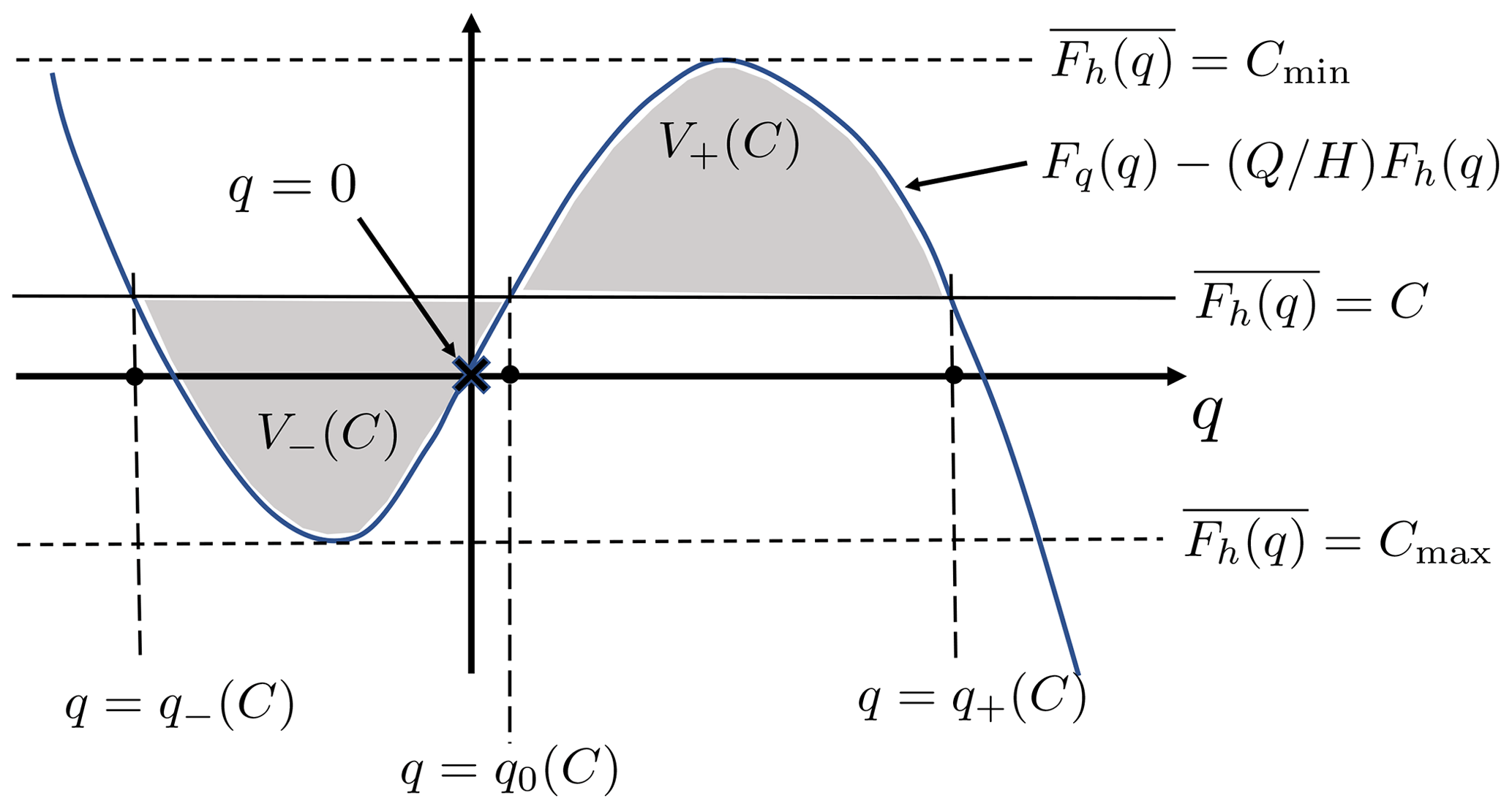
Figure 1 Functions of q controlling the behaviour. The curve shows the function $G_{hq}(q,\stackrel{\mathrm{‾}}{F_h\left(q\right)})=F_q\left(q\right)-(Q/H)F_h\left(q\right)+(Q/H)\stackrel{\mathrm{‾}}{F_h\left(q\right)}$ for the value $\stackrel{\mathrm{‾}}{F_h\left(q\right)}=\mathrm{0}$. q=0, marked by the cross, corresponds to the homogeneous RCE state. Various horizontal straight lines are shown, corresponding to the values $-(Q/H)\stackrel{\mathrm{‾}}{F_h\left(q\right)}$ for different values of $\stackrel{\mathrm{‾}}{F_h\left(q\right)}$. The value of the function $G_{hq}(q,\stackrel{\mathrm{‾}}{F_h\left(q\right)})=F_q\left(q\right)-(Q/H)F_h\left(q\right)+(Q/H)\stackrel{\mathrm{‾}}{F_h\left(q\right)}$ corresponds to the vertical difference between the curve and the relevant line. For $C_{\min }<\stackrel{\mathrm{‾}}{F_h\left(q\right)})<C_{\max }$ the curve and the straight line intersect at three values of q, denoted by $q_{-}\left(\stackrel{\mathrm{‾}}{F_h\left(q\right)}\right)$, $q_{\mathrm{0}}\left(\stackrel{\mathrm{‾}}{F_h\left(q\right)}\right)$ and $q_{+}\left(\stackrel{\mathrm{‾}}{F_h\left(q\right)}\right)$. These are indicated in the diagram for $q_{-}\left(\stackrel{\mathrm{‾}}{F_h\left(q\right)}\right)=(C$). The areas between the curve and the straight line in the intervals $\left[q_{-}\right(C),q_{\mathrm{0}}(C\left)\right]$ and $\left[q_{\mathrm{0}}\right(C),q_{+}(C\left)\right]$ are denoted by V₋(C) and V₊(C) respectively. Note that it is clear that there is a choice of C, with $C_{\min }<C<C_{\max }$ such that $V_{-}\left(C\right)=V_{+}\left(C\right)$.

A further question concerns the stability of this steady state. It is clear from Fig. 1 that c_RD is an increasing function of C (the area V₊ increases and the area V₋ decreases as C increases. Suppose that C>C_s so that $V_{+}\left(C\right)>V_{-}\left(C\right)$ and c_RD is positive; i.e. regions of q₊ will propagate into regions of q₋. The consequence will be that the relative area occupied by q₊ will increase, resulting in a decrease in $C=\stackrel{\mathrm{‾}}{F_h\left(q\right)}$, if F_h(q) is a decreasing function of q. Similarly, if C<C_s, then C will increase, indicating that the steady state C=C_s is stable. Note that the above arguments do not describe the process of coarsening but indicate that the two values of q persist, just as they do for the special case of the Allen–Cahn equation and for the system considered by CMWC, suggesting that coarsening is relevant.

We show examples in Sect. 3 to demonstrate that our model system, in regimes where the approximations leading to Eqs. (5) and (7) can be justified, naturally evolves to a piecewise constant configuration with both of the values of q, q₋ and q₊, consistent with the relevant form of $G_{hq}(q,\stackrel{\mathrm{‾}}{F_h\left(q\right)})$.

The strict WTG form of the evolution equation, Eq. (7), suggests that for the system Eqs. (1), (2) and (4), locally q will tend to one of two values, q₋ or q₊, as was the case for the CMWC pure reaction–diffusion system. The distinct additional feature of the system being considered here is that there is an associated pattern of convergence and divergence. The WTG balance in Eq. (2) implies that the divergence ∇⋅u will also tend to one of two values, $D_{-}=-H^{-\mathrm{1}}{F}_h(q_{-},\stackrel{\mathrm{‾}}{h})=Q^{-\mathrm{1}}{F}_q(q_{-},\stackrel{\mathrm{‾}}{h})>\mathrm{0}$ or $D_{+}=-H^{-\mathrm{1}}{F}_h(q_{+},\stackrel{\mathrm{‾}}{h})=Q^{-\mathrm{1}}{F}_q(q_{+},\stackrel{\mathrm{‾}}{h})<\mathrm{0}$ respectively. (Note that these estimates of convergence in moist regions and divergence in dry regions are the basis for the discussion above concerning the introduction of the parameter ϵ to control the magnitude of advective nonlinearity.) Assume that the corresponding values of ∇⋅u are $-D_{-}<\mathrm{0}<D_{+}$. Since area-integrated ∇⋅u is zero, we expect that the areas A₋ and A₊ filled by dry regions and moist regions respectively satisfy $A_{-}{D}_{-}\sim A_{+}{D}_{+}$.

This non-zero divergence has no consequence for the evolution of the system under the strict WTG approximation, but if this approximation is relaxed, as is likely to be required at large horizontal scales, then the coupling between moisture and divergence may lead to distinctly different behaviour from that predicted by reaction–diffusion alone. Furthermore, even if WTG can be justified in Eq. (2), the non-zero divergence will potentially be important if the nonlinear advection term ϵu[q]⋅∇q is included, since Eq. (2) implies an advecting velocity field that depends on the distribution of q. A typical velocity at length scale L will be U∼DL. The advective velocity becomes comparable with the reaction–diffusion velocity when $\mathit{ϵ}DL\sim (\mathit{\kappa }\mathit{\mu }{)}^{\mathrm{1}/\mathrm{2}}$; i.e. $L=L_{\mathrm{adv}}\sim (\mathit{\kappa }\mathit{\mu }/D^{\mathrm{2}}{\mathit{ϵ}}^{\mathrm{2}}{)}^{\mathrm{1}/\mathrm{2}}$. Since moist regions are associated with convergence and dry regions with divergence, the effect of advection will be to reduce the areas of moist regions relative to those of dry regions. This suggests that in a steady state the reaction–diffusion velocity c_RD has to be positive rather than zero, i.e. that $V_{+}>V_{-}$ rather than $V_{+}=V_{-}$. It also suggests that the values of q in both moist and dry regions are increased relative to their values without the advective nonlinearity. On scales larger than those of a single aggregated region, the combination of regions of divergence of opposite signs will generate a large-scale velocity field. Nonlinear advection will therefore cause aggregation when there is a high density of distinct convergent regions, on a timescale of $\mathit{ϵ}/D$. The advective regime of aggregation becomes dominant for length scales L>L_adv. The consequence of this is illustrated in Sect. 3.2.

We can also now give a better estimate for T_q and hence the scale at which WTG will fail. In the linear instability phase a possible estimate is $T_q\sim {\mathit{\mu }}^{-\mathrm{1}}$. However in the nonlinear aggregation phase a potentially more relevant estimate is $T_q\sim L/c_{\mathrm{RD}}$; i.e. the timescale increases as the length scale increases. In this case where $\mathit{\alpha }=\mathit{\lambda }=f=\mathrm{0}$, then for WTG the first estimate would require $L\ll c{\mathit{\mu }}^{-\mathrm{1}}$. However the second estimate would require $L\ll cL/c_{\mathrm{RD}}$, suggesting that if c_RD≪c, then in the nonlinear aggregation phase the WTG description remains valid at all scales; i.e. aggregation simply proceeds until the length scale is the largest allowed by the geometry.

3 Numerical simulations in the WTG regime

3.1 Model details

The model equations defined above in Eqs. (1)–(3) can be integrated numerically, and in this section we use this to confirm the previous results and further investigate model behaviour. Numerical details are given in Appendix A. Recall that the thickness variable h and the moisture variable q represent the departure from the spatially homogeneous RCE state. In all simulations reported below the initial condition is taken to be u=0, h=0 and q small with $\left|q\right|\ll \left|q_{\pm }\right|$. The values of q are chosen randomly at each grid point.

The theoretical discussion in the previous section does not depend on the precise form of the functions F_h and F_q appearing in Eqs. (2) and (3) respectively, requiring only that they together lead to a bistable moisture equation, Eq. (7). However, in order to investigate the behaviour numerically we need to define these forms explicitly. For illustrative purposes we use a piecewise linear construction, with

$$\begin{array}{}\text{(12)}& {\displaystyle }{F}_q\left(q\right)=-{\mathit{\mu }}_{\mathrm{1}}q,\text{(13)}& {\displaystyle }{F}_h\left(q\right)=\left\{\begin{array}{ll}-{\mathit{\mu }}_{\mathrm{2}}{q}_p-{\mathit{\mu }}_{\mathrm{1}}(q-q_p),& q>q_p\\ -{\mathit{\mu }}_{\mathrm{2}}q,& q_m<q<q_p\\ -{\mathit{\mu }}_{\mathrm{2}}{q}_m-{\mathit{\mu }}_{\mathrm{1}}(q-q_m),& q<q_m.\end{array}\right.\end{array}$$

With ${\mathit{\mu }}_{\mathrm{2}}>{\mathit{\mu }}_{\mathrm{1}}>\mathrm{0}$ this represents larger effective latent heat release of precipitation near to the RCE state. Note that the key quantity $\mathit{\mu }=(\mathrm{d}/\mathrm{d}q)G_{hq}(q;\mathrm{0}){|}_{q=\mathrm{0}}$ is equal to $-{\mathit{\mu }}_{\mathrm{1}}+{\mathit{\mu }}_{\mathrm{2}}Q/H$, which we write as $-{\mathit{\mu }}_{\mathrm{1}}(\mathrm{1}-{\mathit{\mu }}_{\mathrm{2}}Q/H{\mathit{\mu }}_{\mathrm{1}})=-{\mathit{\mu }}_{\mathrm{1}}M$, where M is a normalised gross moist stability of the RCE state. Throughout the paper we choose μ₁ and μ₂ such that M<0, implying that the RCE state is unstable. This simple formulation of F_h and F_q has the advantage that we can easily tune the locations of the fixed points q_± using the parameters q_p and q_m. Note that $q_{+}>q_p$ and $q_{-}<q_m$. Q and H are chosen such that $\mathrm{1}-Q/H>\mathrm{0}$, implying that the fixed points q_p and q_m are stable according to the analysis in Sect. 2.2. We choose $\left|q_p\right|>\left|q_m\right|$, corresponding to a more extreme value of moisture in moist regions than in dry regions. Together with the constraint of zero net heating in steady state, this implies small moist regions with strong upwelling and large dry regions with weak downwelling, as typically observed in convective aggregation (e.g. Muller and Bony, 2015).

Now that the equations are fully defined, the most basic starting point is to consider the system with no rotation or damping, $f=\mathit{\lambda }=\mathit{\alpha }=\mathrm{0}$. The computational domain is taken to be square with sides of length 10⁷ m. We initially take the other parameters in the system as $g=\mathrm{10}\mathrm{m}{\mathrm{s}}^{-\mathrm{2}}$, H=30 m, ${\mathit{\mu }}_{\mathrm{1}}^{-\mathrm{1}}=\mathrm{36}\mathrm{000}\mathrm{s}$, μ₂=3μ₁, $\mathit{\kappa }={\mathrm{10}}^{\mathrm{5}}{\mathrm{m}}^{\mathrm{2}}{\mathrm{s}}^{-\mathrm{1}}$, Q=15 m and $q_p/Q=\mathrm{0.1}$, $q_m/Q=-\mathrm{0.025}$. Note that the corresponding value of M for the RCE state is −0.5. This might be considered a relatively large negative value; e.g. the corresponding value in Sugiyama (2009b) is about −0.05, but the primary reason for this choice is to ensure that the RCE state is unstable, and this value has little effect on the evolution when the system has evolved away from that state. The results of a simulation with GMS of the RCE state increased to −0.05 are shown in Fig. 12. Overall, we argue that the precise values of these parameters are unimportant as here we aim to understand the general behaviour of the system, and indeed the parameters are varied throughout the paper; however the values are chosen to give similar moisture timescales to those deduced from the system studied by Sugiyama (2009b). We use the Craig and Mack (2013) value of $\mathit{\kappa }={\mathrm{10}}^{\mathrm{5}}{\mathrm{m}}^{\mathrm{2}}{\mathrm{s}}^{-\mathrm{1}}$ rather than $\mathit{\kappa }=\mathrm{1.5}\times {\mathrm{10}}^{\mathrm{5}}{\mathrm{m}}^{\mathrm{2}}{\mathrm{s}}^{-\mathrm{1}}$ used by Sugiyama (2009b). The parameter values used in all of the two-dimensional simulations discussed in the paper are given in Table 1. See Sect. 4.3 for a brief discussion of the non-zero values of α, λ and f used later in the paper.

Table 1 Parameters for all examples of two-dimensional simulations shown in the figures. Parameters which remain constant are ${\mathit{\mu }}_{\mathrm{1}}=\mathrm{1}/\mathrm{36}\mathrm{000}{\mathrm{s}}^{-\mathrm{1}}$, ${\mathit{\mu }}_{\mathrm{2}}=\mathrm{1}/\mathrm{12}\mathrm{000}{\mathrm{s}}^{-\mathrm{1}}$, $c^{\mathrm{2}}=\mathrm{300}{\mathrm{m}}^{\mathrm{2}}{\mathrm{s}}^{-\mathrm{2}}$, q_p=0.1Q and $q_m=-\mathrm{0.025}Q$. For 1–9 the f-plane regime is specified on the basis of Fig. 5. For 10–20 (equatorial β-plane simulations), the set of f-plane regimes encountered as f increases from zero is given. For 10–20 the β-plane regime is specified on the basis of Fig. 10. The steady-state column denotes whether or not the parameter values allow convergence to a steady state or, for the β plane, to a steadily propagating state, at large timescales.

3.2 Simulation results

We first consider the case ϵ=0, without nonlinear advection of moisture. The evolution of the moisture distribution with time is shown in Fig. 2. The qualitative behaviour is similar to CMWC. There is an initial adjustment phase on the timescale μ⁻¹ as the small-scale noise grows. During this initial phase, WTG applies only up to $L\sim {\mathit{\mu }}^{-\mathrm{1}}c$, about 10⁶ m for the parameters chosen. Hence distinct regions of enhanced and suppressed moisture on this scale or smaller form, with values corresponding to the effective stable fixed points q_± such that G_hq=0, $\partial G_{hq}/\partial q<\mathrm{0}$.

Figure 2 A series of snapshots of the perturbation moisture distribution $q/Q$ from a numerical integration with no rotation or damping. Note that the final panel in this series is very close to, but has not reached, steady state, which would be a perfectly round moist region.

Once this has occurred, the coarsening process proceeds, with the scale of moist and dry regions slowly evolving, consistent with understanding of the reaction–diffusion system as discussed in the previous section. In particular, the evolution of the boundaries occurs on a slow timescale determined by the reaction–diffusion velocity c_RD and the smaller curvature-associated velocity $\mathit{\kappa }/R$, both of which are smaller than the gravity wave speed c. Hence the WTG approximation continues to hold as the scale of moist and dry regions increases. In this regime the proportion of the domain filled by each of the moist and dry states is changing, so there is a slow evolution of the mean heating $\stackrel{\mathrm{‾}}{F_h\left(q\right)}$. This causes a slow change in the locations of the stable moisture fixed points q_±; however this is on a longer timescale than that determined by G_hq, so the q distribution quickly adjusts to the new stable values. These features of the long-term evolution of the moisture distribution, the rapid adjustment to values of q close to q_± and the subsequent slow evolution of the values of q_± are shown in Fig. 3. This diffusive growth proceeds to the domain scale, when the areas of the regions are such that there is net zero heating and precipitation, and, consistent with theory (Rubinstein et al., 1989), the length of the boundary is minimised (forming either a circular or a band-shaped structure, depending on the geometry of the computational domain). At this point a steady state has been reached.

Figure 3 (a) A histogram of the perturbation moisture distribution $q/Q$, plotted against time. The shading corresponds to the frequency distribution of the moisture values, with darker shades of blue corresponding to higher frequency. The red lines denote the location of q₊ and q₋ calculated as the roots of $G_{hq}(q_{\pm },\stackrel{\mathrm{‾}}{F_h\left(q\right)})=\mathrm{0}$, where the value of the mean heating $\stackrel{\mathrm{‾}}{F_h\left(q\right)}$ is observed from the simulation at each time. Note the slow shift in the values of the fixed points q_± over time, as the mean heating $\stackrel{\mathrm{‾}}{F_h\left(q\right)}$ slowly varies. In panels (b)–(d) the histogram bars have been shown at selected times.

We now briefly consider the system with advective nonlinearity in the moisture equation, ϵ>0. As discussed and noted in Sect. 2.2 above, we expect this to lead to a reduction in the spatial scale of moist regions, an increase in the spatial scale of dry regions and a distinct advective mechanism for aggregation. The simulations show that the effect of the latter is that the system evolves towards a steady state, as was the case for ϵ=0. However advection changes the geometry of this final steady state, as can be seen from the steady-state distributions for different values of ϵ shown in Fig. 4. Unlike with ϵ=0, where the steady state is governed only by reaction–diffusion, the final state is now governed by a balance between reaction–diffusion and advection. The square periodic domain considered in this paper leads to the moisture forming either a band shape or a cross shape. At smaller values of ϵ (ϵ=0.5 is shown), a band forms, and at larger ϵ (ϵ=1 is shown), a cross is preferred. However at intermediate values either shape, according to details of the initial conditions, may be reached and persist. The changes in geometry associated with increasingly strong advection shown here may be relevant to realistic atmospheric flows even if the precise steady-state configurations are not. We emphasise that, as is common to a large class of nonlinear reaction- and diffusion-type problems (e.g. Rubinstein et al., 1989), these steady-state configurations are almost certainly strongly influenced by the domain geometry.

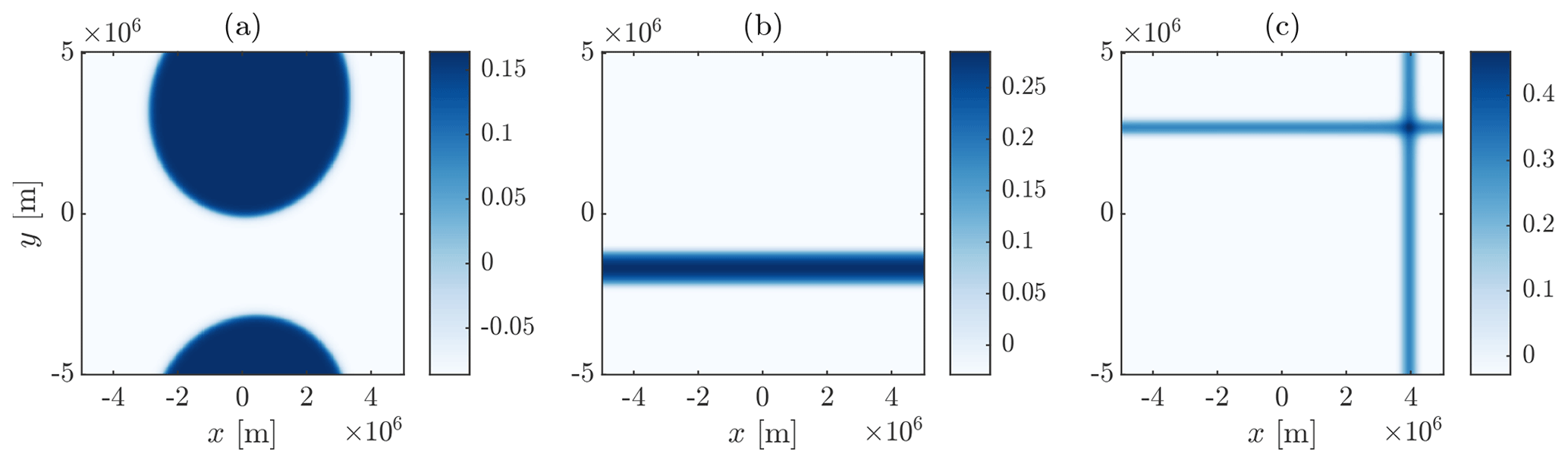
Figure 4 The steady-state moisture distribution, showing $q/Q$, in two-dimensional simulations with no rotation or damping, and (a) ϵ=0, (b) ϵ=0.5 and (c) ϵ=1.

4 Breakdown of WTG and implications for aggregation

When frictional and thermal damping and rotation are included in the system, then, as noted previously, there will be an upper limit L_dyn, depending on the dynamical parameters α, λ and f, on the scale to which WTG balance can apply. It is expected that the coarsening to the domain scale exhibited in the previous section will be substantially modified, and perhaps halted, when the scale L_dyn is reached. Then in Sect. 4.2 we present semi-quantitative scaling arguments that are potentially relevant to the evolution beyond the linear instability phase. We then present results from numerical simulations in Sect. 4.3, both for ϵ=0 and for ϵ>0, including a regime diagram that summarises the overall pattern of behaviour as the dynamical parameters vary.

4.1 Key insights from the linear instability problem

Since the growth of disturbances to the RCE state is the precursor to the coarsening phase, we begin by considering an explicit solution of the linear instability problem when α, λ and f are non-zero.

There have been previous theoretical studies (e.g. Adames et al., 2019) of linear wave propagation and linear instability in systems equivalent to Eqs. (1)–(3), but it is useful to establish some of the basic properties of the particular model system that we consider in this paper. For the case discussed in Sect. 2.2 and illustrated in Sect. 3, where $\mathit{\alpha }=\mathit{\lambda }=f=\mathrm{0}$ and the WTG approximation is valid, the linear stability properties of the RCE state are very straightforward and are determined by the sign of the derivative with respect to q of G_hq(q,0). We consider the linear stability problem in more detail for α, λ and f non-zero values since this gives insight into the behaviour of the full nonlinear system as revealed by numerical simulation. Since the f plane is isotropic, we can assume that perturbations vary only in the x direction. Assuming small-amplitude perturbations of the form $u=\mathrm{\Re }\mathit{\left\{}\widehat{u}\exp \right(\mathit{\sigma }t+ikx\left)\mathit{\right\}}$, with analogous notation for other variables, the linearised forms of Eqs. (1), (2) and (3) are

$$\begin{array}{}\text{(14)}& {\displaystyle }\mathit{\sigma }\widehat{u}-f\widehat{v}=-ikg\widehat{h}-\mathit{\alpha }\widehat{u},\text{(15)}& {\displaystyle }\mathit{\sigma }\widehat{v}+f\widehat{u}=-\mathit{\alpha }\widehat{v},\text{(16)}& {\displaystyle }\mathit{\sigma }\widehat{h}-iHk\widehat{u}=-{\mathit{\mu }}_{\mathrm{2}}\widehat{q}-\mathit{\lambda }\widehat{h},\text{(17)}& {\displaystyle }\mathit{\sigma }\widehat{q}-iQk\widehat{u}=-{\mathit{\mu }}_{\mathrm{1}}\widehat{q}-\mathit{\kappa }{k}^{\mathrm{2}}\widehat{q},\end{array}$$

where ${\mathit{\mu }}_{\mathrm{2}}=-F_h^{\prime }\left(\mathrm{0}\right)$ and ${\mathit{\mu }}_{\mathrm{1}}=-F_q^{\prime }\left(\mathrm{0}\right)$, matching the notation used in Eqs. (13) and (12) respectively. As is standard, these define an eigenvalue problem, the solution of which leads to a dispersion relation in the form of a quartic equation for σ, given explicitly in Appendix B as Eq. (B1).

An important simple case is the strict WTG limit with $\mathit{\alpha }=\mathit{\lambda }=f=\mathrm{0}$. This may be considered directly by neglecting the $\mathit{\sigma }\widehat{h}$ and $-\mathit{\lambda }\widehat{h}$ terms in Eq. (16) and then substituting for $\widehat{u}$ in Eq. (17) to deduce, neglecting the κk² term,

$$\begin{array}{}\text{(18)}& \mathit{\sigma }=-{\mathit{\mu }}_{\mathrm{1}}+{\displaystyle \frac{Q{\mathit{\mu }}_{\mathrm{2}}}{H}}.\end{array}$$

This expression for σ motivates the previously noted definition of the normalised gross moist stability for the moist shallow-water equations,

$$\begin{array}{}\text{(19)}& M=\mathrm{1}-{\displaystyle \frac{Q{\mathit{\mu }}_{\mathrm{2}}}{H{\mathit{\mu }}_{\mathrm{1}}}}.\end{array}$$

As noted previously, in this paper parameter values are chosen such that M<0, implying σ>0 and moisture-mode instability with an inverse timescale $\mathit{\mu }={\mathit{\mu }}_{\mathrm{1}}\left|M\right|$. Note that the WTG approximation applies at small scales, with $k\gg \mathit{\mu }/c$. At large scales, with $k\ll \mathit{\mu }/c$, the moisture adjusts on a timescale shorter than that of the dynamics, and hence a steady-state balance in the moisture equation (Eq. 17), neglecting the term $\mathit{\sigma }\widehat{q}$, is appropriate. (The large-k and small-k limits in this problem correspond to the moisture-mode and gravity-mode limits identified by Adames et al., 2019.) Using the moisture equation to eliminate the moisture dependence in the height equation, Eq. (16), then gives the standard shallow-water equations with the gravity wave speed adjusted from c² to

$$\begin{array}{}\text{(20)}& c^{\mathrm{2}}\left(\mathrm{1}-{\displaystyle \frac{{\mathit{\mu }}_{\mathrm{2}}Q}{H{\mathit{\mu }}_{\mathrm{1}}}}\right)=c^{\mathrm{2}}M.\end{array}$$

This defines the moist gravity wave speed $c_m^{\mathrm{2}}=c^{\mathrm{2}}M$ and implies unstable growth rather than propagation if M<0. M<0 can therefore be identified as a criterion for instability whether or not the WTG approximation is valid. Re-including the effects of moisture diffusion will potentially inhibit instability on length scales comparable to or smaller than $\sqrt{\mathit{\kappa }/{\mathit{\mu }}_{\mathrm{1}}}$.

Analysis of the full dispersion relation, Eq. (B1), given in Appendix B, shows that, if M<0, there is a real positive root for σ only if

$$\begin{array}{}\text{(21)}& \mathit{\kappa }\le (\sqrt{\mathrm{1}-M}-\mathrm{1}{)}^{\mathrm{2}}{\mathit{\mu }}_{\mathrm{1}}{\displaystyle \frac{c^{\mathrm{2}}\mathit{\alpha }}{\mathit{\lambda }({\mathit{\alpha }}^{\mathrm{2}}+f^{\mathrm{2}})}}.\end{array}$$

Note that the final factor represents the square of a length scale which we identify in the following subsection as the dynamical length scale L_dyn. However this does not give complete information on when instability is possible because there may be non-zero complex conjugate roots for σ with a positive real part. Some analytical progress can be made in describing the dependence of roots on the different parameters, but the algebra is complicated. Further details are given in Appendix B.

The behaviour found is illustrated in Fig. 5, which maps out different regions of the (α,λ) plane for a specific choice of κ and for six different choices of f, including f=0. Other parameters, μ₁, μ₂, c², Q and H, take the same values as specified in Sect. 3. The (α,λ) plane may be divided into four regions, each corresponding to a different regime of behaviour. Regime I is where ℜ(σ)>0 occurs for some k only when σ is real. Regimes IIa and IIb are where there are complex σ with ℜ(σ)>0 and with non-zero imaginary parts, and Regime III is where there is no instability, i.e. ℜ(σ)<0 for all k. The distinction between IIa and IIb is that in IIb, σ corresponding to the fastest growth over all k has a non-zero imaginary part.

For f=0 only Regimes I and III are present, and the region of instability simply corresponds to Eq. (21). For non-zero values of f that are not too large, the boundary between Regimes I and III is again described by Eq. (21), but, Regimes IIa and IIb exist in some part of the region α<f. Note that Regimes IIa and IIb are therefore confined to smaller and smaller values of α as f→0. For the largest value of f shown, again only Regimes I and III are present, with Regime I corresponding to Eq. (21). It can be shown in general that if the inequality

$$\begin{array}{}\text{(22)}& f>c({\mathit{\mu }}_{\mathrm{1}}/\mathit{\kappa }{)}^{\mathrm{1}/\mathrm{2}}(\sqrt{\mathrm{1}-M}-\mathrm{1})\end{array}$$

is satisfied, there are no Regimes IIa and IIb, and the transition between stability and instability is fully described by Eq. (21). For the parameters used to generate Fig. 5, the disappearance of regions IIa and IIb between $f=\mathrm{6}\times {\mathrm{10}}^{-\mathrm{5}}$ s⁻¹ and $f={\mathrm{10}}^{-\mathrm{4}}$ s⁻¹ is consistent with Eq. (22).

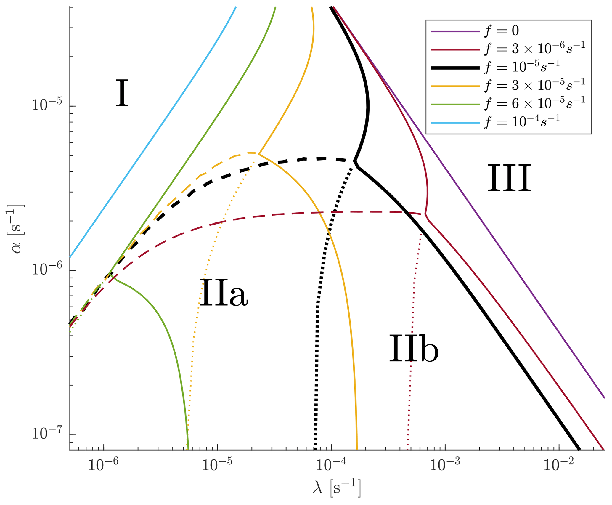
Figure 5 A regime diagram of the linear instability behaviour of the model on the f plane. The black curves mark the boundaries between regimes for a value of $f={\mathrm{10}}^{-\mathrm{5}}{\mathrm{s}}^{-\mathrm{1}}$, and the black regime labels correspond to this curve. The solid black curve marks the boundary between the unstable regimes and the globally stable regime (Regime III). The dashed black curve denotes the boundary separating Regime I on the left, where all unstable modes have zero frequency, and Regime IIa on the right, where some unstable modes have non-zero frequency and are therefore not stationary. The dotted black curve separates Regime IIa on the left from Regime IIb on the right, where the fastest-growing linear mode is no longer stationary. The curves of the four other colours show corresponding boundaries for different values of f, with no equivalent to Regime II appearing when f=0 or when f is sufficiently large. A detailed description of the regime structure is given within the text.

Whilst the parameter dependence that is found in the linear stability problem is complicated, two general rules that seem to hold are, first, increasing κ (unsurprisingly) inhibits instability, and, second, for a given κ, increasing f also tends to inhibit instability; i.e. the region of the (α,λ) plane in which there is instability reduces as these parameters increase. In particular, for any specified non-zero values of α, λ and κ, there is an f_stab such that f>f_stab implies stability. The solid curves shown in Fig. 5 bounding Regime III are therefore, for the chosen value of κ, contours of the function f_stab(λ,α) in the (λ,α) plane. The existence of f_stab is exploited in the description of the equatorial β-plane behaviour in the following section. (Note in particular that f_stab depends on κ as well as on α and λ, but we leave the dependence on κ unstated since in the simulations discussed later, κ is in practice kept fixed, and only α and λ are varied.)

4.2 Dynamical arguments

The description above is focused on the linear instability problem and cannot be assumed to extend to the evolution once the growing unstable disturbances have saturated, e.g. in an aggregation phase. More general insight into the evolution can be obtained by considering possible balances in the equations at horizontal scale L. Assume that the timescale of evolution is T_q. In the linear instability phase $T_q\sim {\mathit{\mu }}^{-\mathrm{1}}$. However after the unstable growth has saturated, T_q may be larger than this. For example, in the aggregation of moist and dry regions described previously, T_q is determined by the diffusivity κ and is large if κ is small.

If α≠0 and λ≠0, then, assuming that $T_q\gg {\mathit{\alpha }}^{-\mathrm{1}},{\mathit{\lambda }}^{-\mathrm{1}}$, a quasi-steady-state balance is possible in the dynamical equations; i.e. u is instantaneously determined by the q field according to the quasi-steady balance,

$$\begin{array}{}\text{(23)}& {\displaystyle }\mathit{\alpha }\mathit{\delta }-f\mathit{\zeta }=-g{\mathrm{\nabla }}^{\mathrm{2}}h,\text{(24)}& {\displaystyle }\mathit{\alpha }\mathit{\zeta }+f\mathit{\delta }=\mathrm{0},\text{(25)}& {\displaystyle }H\mathit{\delta }+\mathit{\lambda }h=F_h\left(q\right),\end{array}$$

where δ is divergence, and ζ is vorticity. In this respect we can identify this case with Regime I in the previous section. Eliminating ζ gives

$$\begin{array}{}\text{(26)}& \mathit{\delta }=-g\mathit{\alpha }({\mathit{\alpha }}^{\mathrm{2}}+f^{\mathrm{2}}{)}^{-\mathrm{1}}{\mathrm{\nabla }}^{\mathrm{2}}h.\end{array}$$

Substituting into Eq. (25) implies that the local h, and hence the local u, is determined by q in a surrounding region of scale:

$$\begin{array}{}\text{(27)}& L_{\mathrm{dyn}}=c(\mathit{\alpha }/\mathit{\lambda }{)}^{\mathrm{1}/\mathrm{2}}({\mathit{\alpha }}^{\mathrm{2}}+f^{\mathrm{2}}{)}^{-\mathrm{1}/\mathrm{2}}.\end{array}$$

This defines a dynamical length scale L_dyn. WTG balance, the local balance between divergence and heating, applies only length scales smaller than L_dyn. On length scales larger than L_dyn, the dominant balance in Eq. (25) is between λh and F_h(q), and hence, from Eq. (26) the divergence is proportional to ∇²F(q) rather than to F(q). Another implication of the above balance, from Eq. (24), is that the flow will be dominated by the rotational component if f≫α and by the irrotational component if f≪α.

The quasi-steady balance above cannot hold when α=0, when Eq. (26) would imply δ=0. However if q is to be maintained away from the q=0 steady state, which is known to be unstable, Eq. (4), neglecting the term multiplied by ϵ, requires δ to be non-zero. This suggests that a distinct dynamical argument is required when α is small, analogous to the distinct nature of Regime II discussed in the previous section. If f≠0, a possible balance assuming a small Rossby number, i.e. that the timescale of the evolution of the q field is much larger than f⁻¹, is

$$\begin{array}{}\text{(28)}& {\displaystyle }-f\mathit{\zeta }=-g{\mathrm{\nabla }}^{\mathrm{2}}h,\text{(29)}& {\displaystyle }{\mathit{\zeta }}_t+f\mathit{\delta }=\mathrm{0},\text{(30)}& {\displaystyle }{h}_t+H\mathit{\delta }+\mathit{\lambda }h=F_h\left(q\right),\end{array}$$

implying

$$\begin{array}{}\text{(31)}& (h-(c^{\mathrm{2}}/f^{\mathrm{2}}){\mathrm{\nabla }}^{\mathrm{2}}h{)}_t+\mathit{\lambda }h=F_h(q),\end{array}$$

that is, a form of the quasi-geostrophic potential vorticity equation with the potential vorticity changing due to the effects of heating F_h(q) and thermal damping. Thus, in this system there are two prognostic equations, one for potential vorticity and one for moisture. In this case it is the second term in the time derivative that corresponds to divergence so that WTG applies if $L\ll (c/f)min(\mathrm{1},(\mathit{\lambda }{T}_q{)}^{-\mathrm{1}/\mathrm{2}})$. Here the length scale appearing is the Rossby radius $c/f$, and the flow can be expected to evolve on the timescale λ⁻¹ at large timescales. Note that in this case the rotational part of the velocity field will be stronger than the divergent part.

In both the above cases it appears that the relation between moist heating and divergence becomes non-local at a sufficiently large scale, L_dyn, when α is large enough to bring the dynamical balance to a quasi-steady state and $c/f$ when α is smaller. Therefore the aggregation behaviour seen previously is likely to be halted, or at least strongly modified, when these scales are reached. In Sect. 4.3 below the nature of this modification is examined by numerical simulation.

The scale L_dyn defined above decreases as f increases, suggesting that the scale of aggregated moist and dry regions will also decrease as f increases. Furthermore, the underlying instability of the RCE state requires WTG dynamics to apply, and L_dyn therefore also represents an upper limit on the scale of the instability. As f increases, L_dyn will reduce to the diffusion scale $\sqrt{\mathit{\kappa }/\mathit{\mu }}$, and the instability of the RCE state will disappear. This provides an estimate for f_stab,

$$\begin{array}{}\text{(32)}& \sqrt{{\displaystyle \frac{\mathit{\alpha }}{\mathit{\lambda }}}}{\displaystyle \frac{c}{\sqrt{f_{\mathrm{stab}}^{\mathrm{2}}+{\mathit{\alpha }}^{\mathrm{2}}}}}=\mathrm{\Gamma }\sqrt{{\displaystyle \frac{\mathit{\kappa }}{\mathit{\mu }}}},\end{array}$$

where Γ is a non-dimensional parameter. The expression Eq. (21), provided by the linear stability calculation, is consistent with this reasoning and provides an explicit expression for Γ as equal to $\sqrt{-M}/(\sqrt{\mathrm{1}-M}-\mathrm{1})$. For the case when α is small, corresponding to Regime II, we have no expression for L_dyn or for the boundary of stability between Regimes II and III in Fig. 5, so a corresponding analytic result has not been determined. We do expect a qualitatively similar situation where the system is stabilised by diffusion once the maximum length scale L_dyn becomes sufficiently small. However, the behaviour, as f changes, of the boundary between Regime IIb and Regime III shown in Fig. 5 is geometrically complicated. This suggests that an easily interpretable expression for the entire form of the boundary will be difficult to find.

4.3 Numerical simulations

The link between the maximum length scale L_dyn, determined by non-zero values of f, α and λ, over which WTG is expected to apply and the spatial scale of aggregation are now illustrated using numerical simulation. The same numerical scheme as in Sect. 3 is used. The parameters, μ₁, μ₂, c², Q and H, take the same values as specified in Sect. 3, unless otherwise stated. Additionally, f, α and λ are chosen so that there is linear instability, corresponding to Regimes I, IIa and IIb in Fig. 5. Recall that details of the parameter values chosen for these simulations are given in Table 1. The values of f are chosen for illustrative purposes ($f={\mathrm{10}}^{-\mathrm{5}}{\mathrm{s}}^{-\mathrm{1}}$ corresponds to about 5°). Representative values of α and λ are chosen to be similar to those in other papers on large-scale tropical dynamics; e.g. Sugiyama (2009b) takes $\mathit{\alpha }=\mathrm{2}\times {\mathrm{10}}^{-\mathrm{6}}{\mathrm{s}}^{-\mathrm{1}}$ and $\mathit{\lambda }=\mathrm{5}\times {\mathrm{10}}^{-\mathrm{7}}{\mathrm{s}}^{-\mathrm{1}}$, and Adames and Wallace (2014) take $\mathit{\alpha }={\mathrm{10}}^{-\mathrm{6}}{\mathrm{s}}^{-\mathrm{1}}$ and $\mathit{\lambda }={\mathrm{10}}^{-\mathrm{6}}{\mathrm{s}}^{-\mathrm{1}}$, Adames and Kim (2016) take $\mathit{\alpha }=\mathrm{3}\times {\mathrm{10}}^{-\mathrm{6}}{\mathrm{s}}^{-\mathrm{1}}$ and $\mathit{\lambda }=\mathrm{3}\times {\mathrm{10}}^{-\mathrm{6}}{\mathrm{s}}^{-\mathrm{1}}$, but we deliberately diverge from these representative values in some simulations to investigate the effect of varying α and λ in different ways. Note that the justification of values for linear friction coefficients, or indeed the inclusion of linear friction at all, in models for tropical circulation remains a topic of active discussion (e.g. Romps, 2014).

4.3.1 ϵ=0 (advective nonlinearity excluded)

We begin with ϵ=0, i.e. excluding nonlinear advection of moisture. A selection of time series of the moisture distribution of the system for different choices of f, α and λ is shown in Fig. 6, with each simulation corresponding to a row. In all cases the moisture field q was initialised with small-scale random noise. In the first case, in row A, corresponding to Regime I in the (α,λ) plane shown in Fig. 5, the system initially evolves similarly to the case without damping or rotation, with the formation of distinct moist regions, which evolve and enlarge through aggregation. However the aggregation does not proceed to the domain scale but halts at a smaller scale, with quasi-steady circular moist regions. This is as expected from the previous dynamical discussion. The inclusion of non-zero f, α and λ implies that WTG balance can hold only up to the scale L_dyn and aggregation halts at this scale. Other simulations with f, α and λ corresponding to Regime I in Fig. 5 show similar evolution.

Figure 6 A series of snapshots of the perturbation moisture distribution $q/Q$ of a two-dimensional simulation, this time with rotation and damping. Row A corresponds to case I in Sect. 4.1. This has $f={\mathrm{10}}^{-\mathrm{5}}{\mathrm{s}}^{-\mathrm{1}}$ and $\mathit{\alpha }=\mathit{\lambda }=\mathrm{4}\times {\mathrm{10}}^{-\mathrm{6}}{\mathrm{s}}^{-\mathrm{1}}$, giving $L_{\mathrm{dyn}}=\mathrm{1.6}\times {\mathrm{10}}^{\mathrm{6}}\mathrm{m}$. Rows B and C correspond to case II. Row B has $\mathit{\alpha }={\mathrm{10}}^{-\mathrm{7}}{\mathrm{s}}^{-\mathrm{1}}$ and $\mathit{\lambda }={\mathrm{10}}^{-\mathrm{6}}{\mathrm{s}}^{-\mathrm{1}}$, and C has $\mathit{\alpha }={\mathrm{10}}^{-\mathrm{6}}{\mathrm{s}}^{-\mathrm{1}}$ and $\mathit{\lambda }={\mathrm{10}}^{-\mathrm{4}}{\mathrm{s}}^{-\mathrm{1}}$.

Rows B and C in Fig. 6 correspond to Regime II in the (λ,α) plane, with B corresponding to IIa and C to IIb. For case B there is again an initial segregation and then an aggregation process, leading to distinct moist and dry regions at some finite scale. However, the long-time distribution is no longer stationary but continues to evolve in time (without there being any further systematic increase in scale). In case C, whilst there is segregation, there is no clear aggregation stage, and the moist and dry regions evolve in time in a manner that is more wave-like than that seen in case B.

To establish that the division of the (α,λ) plane, originally motivated by the linear instability properties, provides a useful guide on the behaviour of the ultimate nonlinear evolution, Fig. 7 repeats the depiction of the (λ,α) plane shown previously for a single value of f, with superimposed symbols indicating whether the nonlinear evolution was aggregated and quasi-steady, as in case A above; aggregated and unsteady, as in case B; or propagating, as in case C. Regime IIa (case B) has been split into two sub-regimes, with a slow regime corresponding to transitional behaviour in which aggregated regions form, but propagation is sufficiently slow so that these remain round.

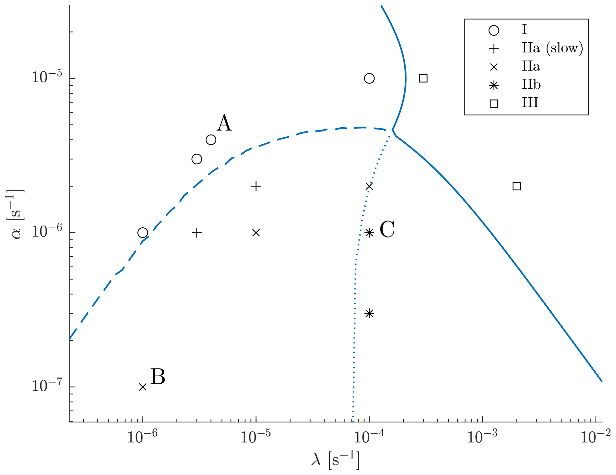
Figure 7 The regime diagram curve for $f={\mathrm{10}}^{-\mathrm{5}}{\mathrm{s}}^{-\mathrm{1}}$ from Fig. 5, overlaid with the observed regimes from numerical simulations. Each point marked in the figure corresponds to the parameter values for a simulation, which was then categorised into one of four regimes. The points corresponding to the moisture distributions shown in Fig. 6 are labelled A, B and C.

A possible interpretation of the apparent relation between the properties of the linear instability problem and the evolution observed in the numerical simulations is as follows. In Regime I, as illustrated by simulation A, the linear instability behaviour is essentially that described by the WTG approximation, with the relevant unstable mode having real σ. Therefore the system evolves through the instability to the segregated state determined by the bistability. In Regime IIa, as illustrated by simulation B, the relevant unstable mode is similar to that in A, with σ real, and the process of segregation is correspondingly similar. However the existence of slower-growing propagating (complex σ) unstable modes at larger scales is relevant to the nonlinear evolution post-segregation (even if the linear instability modes themselves do not provide a complete description of the behaviour). (A reduced mathematical model describing the evolution of the segregated state might make this relevance clearer.) In Regime IIb, illustrated by simulation C, there is a pair of the fastest-growing modes with complex conjugate σ rather than a single mode with real σ, and the mechanism for growth is therefore completely different from that described by the WTG approximation. In fact, these modes are better regarded as moisture-destabilised inertial waves and are not moisture modes since they rely on the fact that the dynamics is not slaved to the moisture field. Consequentially the nonlinear evolution is not so clearly a segregation into the two states allowed by bistability and instead is better characterised as an evolving field of nonlinear moisture-inertial waves. Note that systematic propagation in case C and the clear anisotropy of the instantaneous q distribution visible in Fig. 6i are an indication of spontaneous symmetry breaking rather than any systematic anisotropy of the system as specified.

We now focus on the behaviour of the model with parameters chosen from Regime I, where there is aggregation to a quasi-steady state. The behaviour can be usefully summarised by using the spatial autocorrelation. The autocorrelation scale, L_auto, is defined as the minimum radius at which the spatial autocorrelation is a factor of $\mathrm{1}/e$ less than its maximum value. The time evolution of L_auto for simulations with various damping and rotation rates, as well as diffusivities, is shown in Fig. 8.

Cases (a) and (b) have $\mathit{\alpha }=\mathit{\lambda }=f=\mathrm{0}$, so, as previously demonstrated in Sects. 2.2–3, aggregation is expected to eventually proceed to the domain scale. The evolution of L_auto for both case (a) and case (b) is consistent with this expectation. For case (b), L_auto reaches a limiting value within the time period shown in the figure. For case (a), a limiting value is not reached, but L_auto continues to increase throughout the period shown. The difference between (a) and (b) can be explained by the fact that κ for (b) is 4× larger than that for (a), therefore recalling the established theory on reaction–diffusion systems noted in Sect. 2.2 that aggregation proceeds more rapidly as κ increases.

Other cases have non-zero values of α, λ and f. All these show an approach to a finite limiting value, indicating that aggregation ceases. A candidate value for the length scale at which this occurs is $L_{\mathrm{dyn}}=c(\mathit{\alpha }/\mathit{\lambda }{)}^{\mathrm{1}/\mathrm{2}}({\mathit{\alpha }}^{\mathrm{2}}+f^{\mathrm{2}}{)}^{-\mathrm{1}/\mathrm{2}}$. The corresponding values deduced from Fig. 8 are consistent with this expression in the sense that the ordering as parameters are changed is consistent with the expression. Note in particular that for a given α and λ, the scale is smaller with f>0 than it is with f=0.

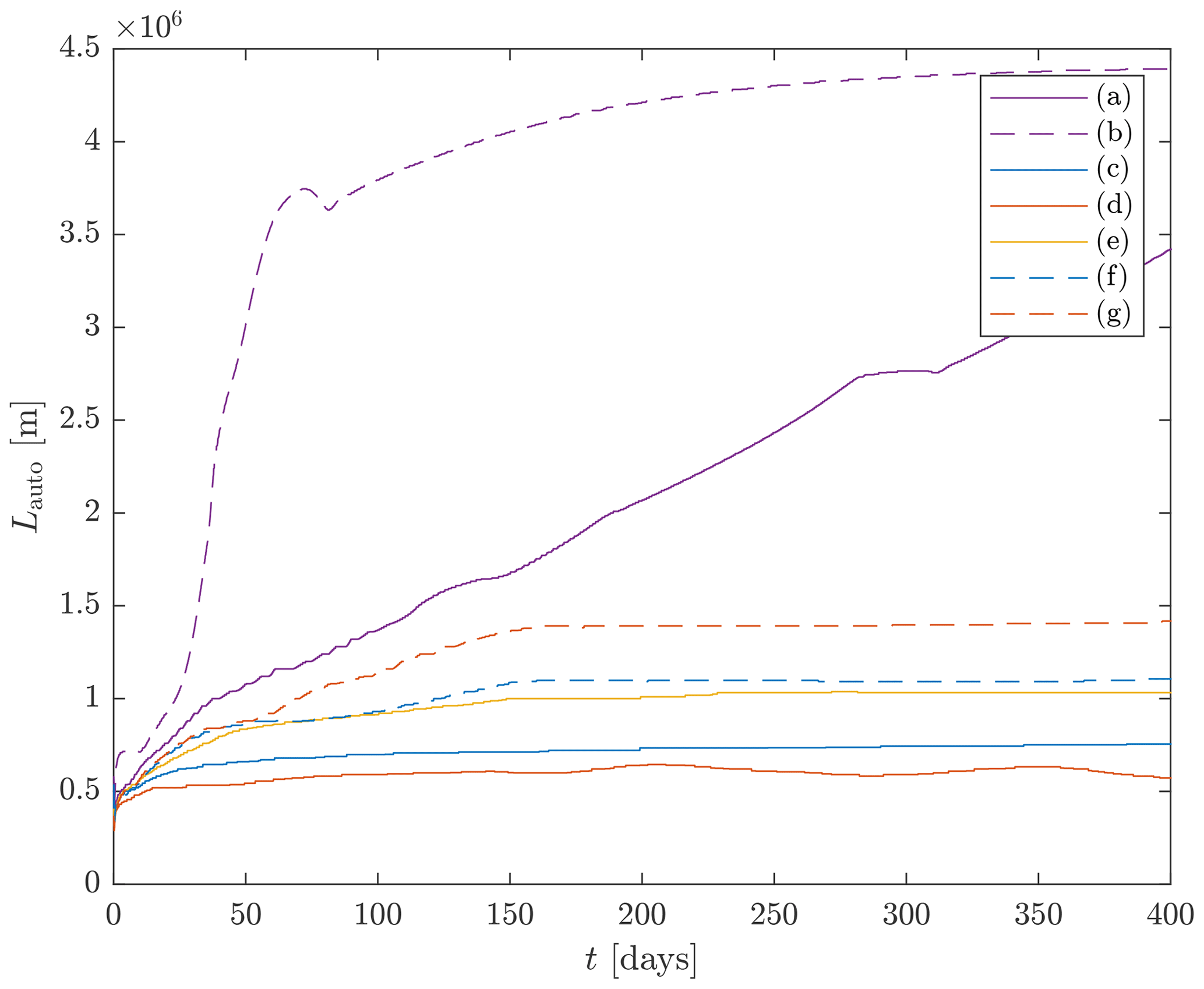
Figure 8 A measure of autocorrelation length scale plotted against time for various parameter values, within case I. Curves (a) and (b) have $\mathit{\alpha }=\mathit{\lambda }=f=\mathrm{0}$. Curve (a) has $\mathit{\kappa }={\mathrm{10}}^{\mathrm{5}}{\mathrm{m}}^{\mathrm{2}}{\mathrm{s}}^{-\mathrm{1}}$, and (b) has $\mathit{\kappa }=\mathrm{4}\times {\mathrm{10}}^{\mathrm{5}}{\mathrm{m}}^{\mathrm{2}}{\mathrm{s}}^{-\mathrm{1}}$. Curve (c) has $f={\mathrm{10}}^{-\mathrm{5}}{\mathrm{s}}^{-\mathrm{1}}$, $\mathit{\alpha }=\mathit{\lambda }=\mathrm{4}\times {\mathrm{10}}^{-\mathrm{6}}{\mathrm{s}}^{-\mathrm{1}}$ and $\mathit{\kappa }={\mathrm{10}}^{\mathrm{5}}{\mathrm{m}}^{\mathrm{2}}{\mathrm{s}}^{-\mathrm{1}}$. Curves (d) and (e) show the effect of reducing α and λ respectively by a factor of 4. Curves (f) and (g) have the same parameters as (c) and (d) respectively but with f=0. The length scale varies consistently with the value of L_dyn.

4.3.2 ϵ>0 (advective nonlinearity included)

The effects of advective nonlinearity in the presence of non-zero f, α and λ are illustrated in Fig. 9. Note that each of these cases has (λ,α) corresponding to Regime I. We have previously noted that the effect of advective nonlinearity is in the two-dimensional case to give moist regions that are more filamentary than quasi-circular. (For example, recall the steady-state moisture distributions, where aggregation has proceeded to the domain scale, for $\mathit{\alpha }=\mathit{\lambda }=f=\mathrm{0}$ shown in Fig. 4.) The effect of non-zero α, λ and f is both to limit any aggregation to a finite scale and to determine the flow pattern resulting from the moisture distribution. When f≠0 this flow has a substantial rotational component, and the advective effect of this on the filamentary moisture structures is apparent in Fig. 9a and b. The example with f=0, shown in Fig. 9c, where the advecting flow is irrotational, is distinctly different, with any curvature of the filamentary structures being weaker and resulting from deformation by a spatially structured irrotational flow. As has been noted previously, advective narrowing of moist regions means that the maximum magnitude q is affected by diffusion and not simply equal to the predicted value q₊.

Figure 9 The perturbation moisture distribution, $q/Q$, after 400 d for a selection of two-dimensional nonlinear simulations. Panel (a) has $f=\mathit{\alpha }=\mathit{\lambda }={\mathrm{10}}^{-\mathrm{6}}{\mathrm{s}}^{-\mathrm{1}}$, (b) has $f=\mathit{\alpha }=\mathit{\lambda }={\mathrm{10}}^{-\mathrm{5}}{\mathrm{s}}^{-\mathrm{1}}$ and (c) has $\mathit{\alpha }=\mathit{\lambda }={\mathrm{10}}^{-\mathrm{5}}{\mathrm{s}}^{-\mathrm{1}}$ but f=0.

5 Equatorial β plane

In this section we consider the model on the equatorial β plane, i.e. with f=βy. It has been shown that on the f plane aggregation tends to be inhibited by rotation in two ways: (i) the upper limit of the scale for the underlying instability of the system is a decreasing function of f, and the lower limit is an increasing function of κ; therefore when κ is non-zero, the instability disappears altogether for $f>f_{\mathrm{stab}}=\mathit{\beta }{y}_{\mathrm{stab}}$, with the latter equality defining y_stab. (ii) The upper limit on the aggregation scale is a decreasing function of f. This suggests the possibility on the β plane of disturbances largely confined to some equatorial band with $\left|y\right|<y_{\mathrm{stab}}$. Such disturbances do indeed form, and we proceed to describe their behaviour.

The regime diagram shown in Fig. 5 in Sect. 4.1 provides some insight into how the dynamics might vary with latitude. At the Equator, with f=0, either Regime I or Regime III must apply, with Regime III implying that the RCE state is stable. For large f Regime III applies. Whether or not the transition from Regime I to Regime III passes through Regime II will be determined by the values of α and λ. Generally speaking this will occur when $\mathit{\alpha }/\mathit{\lambda }$ is relatively small. If Regime II is encountered then this is likely to manifest as more complicated behaviour (recall Fig. 6) as y_stab is approached. However we see later in this section that there are effects on the β plane that are not captured by the f-plane behaviour as described in Sect. 4.

It has been noted in the previous section that, on the f plane, whilst there was sometimes evidence of a selection of a preferred direction (recall Fig. 6c), this selection is purely random. On the β plane, however, there is a genuine east–west asymmetry, e.g. as manifested in the well-known Matsuno–Gill steady response to localised heating, which has been generalised by Wu et al. (2001) to the case where α and λ are not equal. It is of particular interest to determine whether this leads to zonal propagation of moist and dry regions and how such propagation varies with model parameters.

We begin this section by discussing an adjustment to the previous constant-f dynamical arguments and its impact on the local distribution of aggregated regions. We then describe the effects of the larger-scale equatorial circulation. Following this, we discuss the behaviour of a series of numerical experiments, in both the ϵ=0 and the ϵ>0 cases.

5.1 Implications of equatorial β-plane dynamics

Much of the scale analysis of the f-plane equations presented in Sect. 4.2 was based on a quasi-steady balance in the dynamical equations, which led to the relation (Eq. 26) between δ and h and hence an estimate $L_{\mathrm{dyn}}=c(\mathit{\alpha }/\mathit{\lambda }{)}^{\mathrm{1}/\mathrm{2}}({\mathit{\alpha }}^{\mathrm{2}}+f^{\mathrm{2}}{)}^{-\mathrm{1}/\mathrm{2}}$ for the scale on which WTG breaks down, serving as an effective upper limit on the scale of aggregation. The same approach of assuming a quasi-steady balance in the dynamical equations is now applied to the β plane. The scale L_dyn as defined previously is still useful but will now vary with latitude. It is convenient to use the notation L_dyn,f to represent the value of L_dyn for a particular value of f. At this stage it is also useful to note that the system being considered has no imposed inhomogeneity in x, i.e. in longitude, and there is therefore no systematic change in the character of the disturbances in x; i.e. there is representation of a “warm-pool” range of longitudes in which moisture has a stronger role in the dynamics than elsewhere. Correspondingly, any below-mentioned reference to integration over the domain refers to the entire domain and is not restricted to a particular range of x values.

The balance in Eq. (26) must be modified on the β plane because $\partial f/\partial y$ is non-zero and becomes

$$\begin{array}{}\text{(33)}& \mathit{\delta }=-{\displaystyle \frac{g\mathit{\alpha }}{{\mathit{\alpha }}^{\mathrm{2}}+f^{\mathrm{2}}}}{\mathrm{\nabla }}^{\mathrm{2}}h+{\displaystyle \frac{g\mathit{\beta }}{f^{\mathrm{2}}+{\mathit{\alpha }}^{\mathrm{2}}}}\widehat{\mathit{n}}\cdot \mathrm{\nabla }h,\end{array}$$

where $\mathit{\beta }=\partial f/\partial y$ and $\widehat{\mathit{n}}=({\mathit{\alpha }}^{\mathrm{2}}-f^{\mathrm{2}},\mathrm{2}f\mathit{\alpha })/(f^{\mathrm{2}}+{\mathit{\alpha }}^{\mathrm{2}})$ is a unit vector. Substituting Eq. (33) into the thickness equation (Eq. 2) gives the steady response to a heating as

$$\begin{array}{}\text{(34)}& \mathit{\lambda }h+H\mathit{\delta }=\mathit{\lambda }h-{\displaystyle \frac{gH\mathit{\alpha }}{{\mathit{\alpha }}^{\mathrm{2}}+f^{\mathrm{2}}}}{\mathrm{\nabla }}^{\mathrm{2}}h+{\displaystyle \frac{gH\mathit{\beta }}{f^{\mathrm{2}}+{\mathit{\alpha }}^{\mathrm{2}}}}\widehat{\mathit{n}}\cdot \mathrm{\nabla }h=F_h\left(q\right).\end{array}$$

One important difference from the corresponding equations for the f plane is that there is now a preferred direction in the relation between δ and h, allowing a systematic anisotropy. A second difference is that the coefficients in the equations are now functions of y. A local analysis, treating f as constant, may therefore not always be valid. The expressions above suggest a change in the character of the system when the length scale is larger than $\mathit{\alpha }/\mathit{\beta }$. Below this scale, the first, isotropic term in Eq. (33) is dominant, and, furthermore, the coefficient appearing in this term does not vary significantly on this scale, so a local description will be valid. For length scales larger than $\mathit{\alpha }/\mathit{\beta }$, however, the second term is dominant, suggesting significant anisotropy in the dynamics. The coefficients and the vector $\widehat{\mathit{n}}$ will also vary significantly with f, so significant latitudinal variation is expected, and, more fundamentally, a local description may not be valid.

Along with the above it must be taken into account that aggregation is initiated by instability of the RCE state and that this instability is confined to $\left|y\right|<y_{\mathrm{stab}}$. Additionally, whilst it is expected that moisture anomalies are largely confined within this region, note that Eq. (34) implies that dynamical effects extend outside, on a length scale of $L_{\mathrm{dyn},f=\mathit{\beta }{y}_{\mathrm{stab}}}$. When M is large and negative, Eq. (32) suggests this scale is $\sqrt{\mathit{\kappa }/\mathit{\mu }}$: a diffusive response extending outside of the unstable equatorial region. When M is closer to zero, however, this length scale may be significantly larger.

The f-plane analysis predicts L_dyn as an upper limit on the scale for aggregation. This suggests $L_{\mathrm{dyn},f=\mathrm{0}}=c/\sqrt{\mathit{\lambda }\mathit{\alpha }}$ as the corresponding scale at the Equator on the β plane. Therefore, on the basis of the arguments above, aggregation at the Equator may be isotropic if $L_{\mathrm{dyn},f=\mathrm{0}}<\mathit{\alpha }/\mathit{\beta }$ and $y_{\mathrm{stab}}>L_{\mathrm{dyn},f=\mathrm{0}}$. If the second condition is not satisfied then the geometry will not allow isotropy. Furthermore, since $L_{\mathrm{dyn},f=\mathit{\beta }y}$ is a decreasing function of y, isotropy will extend to y=y_stab, but the characteristic length scales will decrease as $\left|y\right|$ increases. In other words, we expect the aggregation to be qualitatively similar to the f-plane case, except that it will be confined to a region slightly larger than $\left|y\right|<y_{\mathrm{stab}}$, and the characteristic length scale will vary with y. If $L_{\mathrm{dyn},f=\mathrm{0}}<\mathit{\alpha }/\mathit{\beta }$ and $y_{\mathrm{stab}}<L_{\mathrm{dyn},f=\mathrm{0}}$, on the other hand, then the aggregated structures in moisture will be largely confined to $\left|y\right|<y_{\mathrm{stab}}$ and therefore extended in x relative to their scale in y. However the dynamical signatures will extend to $\left|y\right|=L_{\mathrm{dyn},f=\mathrm{0}}$. This suggests two distinct regimes of behaviour in a parameter space defined by $y_{\mathrm{stab}}\mathit{\beta }/\mathit{\alpha }$ and $L_{\mathrm{dyn},f=\mathrm{0}}\mathit{\beta }/\mathit{\alpha }=c\mathit{\beta }{\mathit{\alpha }}^{-\mathrm{3}/\mathrm{2}}{\mathit{\lambda }}^{-\mathrm{1}/\mathrm{2}}$. We label these Regime A ($L_{\mathrm{dyn},f=\mathrm{0}}<\mathit{\alpha }/\mathit{\beta }$, $L_{\mathrm{dyn},f=\mathrm{0}}<y_{\mathrm{stab}}$) and Regime E ($L_{\mathrm{dyn},f=\mathrm{0}}<\mathit{\alpha }/\mathit{\beta }$, $y_{\mathrm{stab}}<L_{\mathrm{dyn},f=\mathrm{0}}$). These two regimes are shown in the $(L_{\mathrm{dyn},f=\mathrm{0}},y_{\mathrm{stab}})$ plane in Fig. 10. We add further regimes to this diagram and discuss them in more detail below.

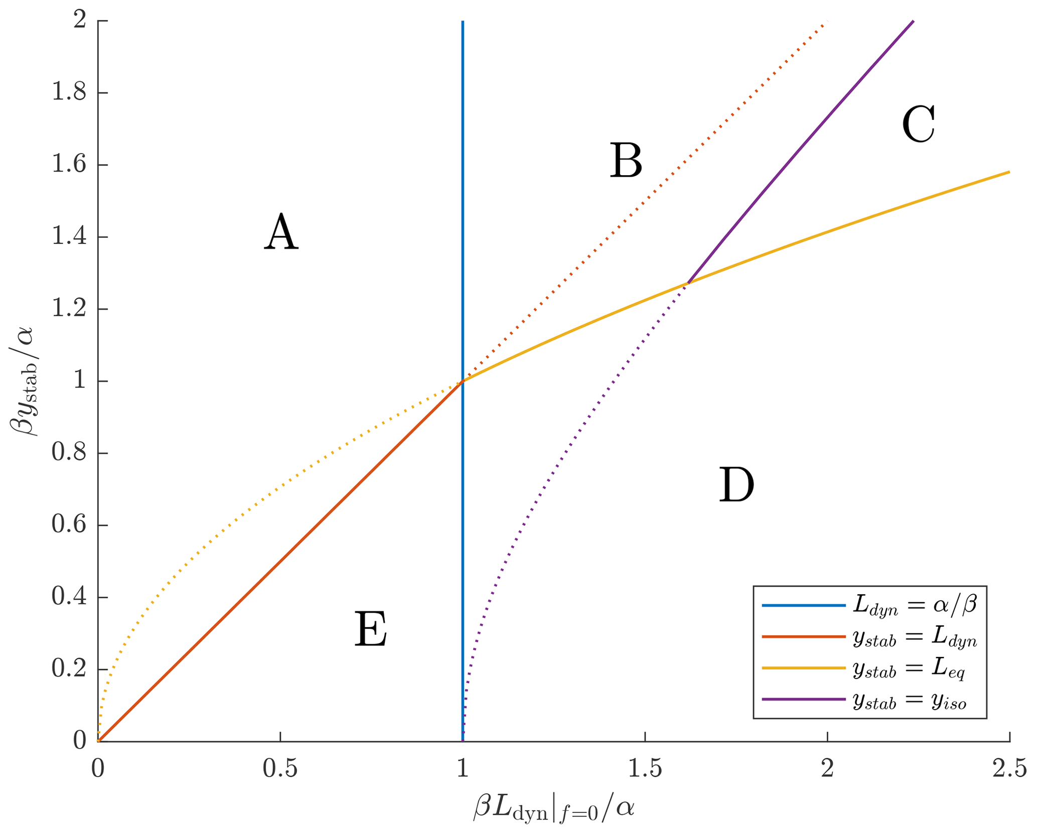
Figure 10 A schematic plot of the expected regimes of behaviour of our model on the equatorial β plane, shown against varying the latitudinal scale of the equatorial wave response $L_{\mathrm{dyn}}{|}_{f=\mathrm{0}}=c/\sqrt{\mathit{\alpha }\mathit{\lambda }}$ and the latitudinal limit of bistability y_stab, both in units of $\mathit{\alpha }/\mathit{\beta }$. The solid lines denote regime boundaries, and the remainder of each curve is dotted. The equations defining each of the regime boundaries are given in the legend. These are discussed in further detail in the main text. A brief summary of the characteristics of each regime is as follows. Regime A – the local f-plane analysis is valid, and isotropic aggregated regions extend to y_stab. Regime B – aggregated regions are on the Equator with y scale L_eq, and a transition to isotropic aggregated regions occurs at larger $\left|y\right|$. Regime C – aggregated regions are on the Equator with y scale L_eq, and anisotropic aggregated regions are at larger $\left|y\right|$. Regime D – aggregated regions are centred on the Equator with y scale L_eq. Regime E – aggregated regions are centred on the Equator with y scale y_stab. In Regimes A, B and C there are multiple aggregated regions in latitude. Regions at different latitudes propagate in the x direction at different velocities. In Regimes D and E all aggregated regions are centred on the Equator, and there is coherent propagation in the x direction.

We now consider the case where $L_{\mathrm{dyn},f=\mathrm{0}}>\mathit{\alpha }/\mathit{\beta }$. The non-isotropic terms in Eqs. (33) and (34) must be taken into account. Furthermore, close to the Equator, a local analysis is no longer adequate. A natural y scale close to y=0, obtained by requiring a balance between the first and second terms in the middle expression in Eq. (34), is $L_{\mathrm{eq}}=(c/\mathit{\beta }{)}^{\mathrm{1}/\mathrm{2}}(\mathit{\alpha }/\mathit{\lambda }{)}^{\mathrm{1}/\mathrm{4}}$, as obtained by Wu et al. (2001) in their generalisation of the Matsuno–Gill problem. The corresponding x scale, however, agrees with the length scale from the local analysis at the Equator, $L_{\mathrm{dyn},f=\mathrm{0}}$. Note that $L_{\mathrm{eq}}=\sqrt{L_{\mathrm{dyn},f=\mathrm{0}}\mathit{\alpha }/\mathit{\beta }}$ and that L_eq therefore always lies between $\mathit{\alpha }/\mathit{\beta }$ and L_dyn, i.e. when $L_{\mathrm{dyn},f=\mathrm{0}}>\mathit{\alpha }/\mathit{\beta }$, $\mathit{\alpha }/\mathit{\beta }<L_{\mathrm{eq}}<L_{\mathrm{dyn},f=\mathrm{0}}$. The structure of Eq. (34) implies that a moisture anomaly localised within region $\left|y\right|<L_{\mathrm{eq}}$ will force dynamical anomalies that extend across the region $\left|y\right|\sim L_{\mathrm{eq}}$. This implies a distinct Regime D ( $\mathit{\alpha }/\mathit{\beta }<L_{\mathrm{dyn},f=\mathrm{0}}$, y_stab<L_eq) similar to Regime E, with latitudinally confined moisture anomalies driving broader dynamical anomalies.

Now consider $(L_{\mathrm{dyn},f=\mathrm{0}}>\mathit{\alpha }/\mathit{\beta }$, y_stab>L_eq). In this case, since y_stab>L_eq, the unstable region is large enough to allow multiple aggregated structures in the y direction. Since we have $L_{\mathrm{dyn},f=\mathrm{0}}>\mathit{\alpha }/\mathit{\beta }$, there is anisotropy at the Equator, but since L_dyn is a decreasing function of f, the anisotropic region is expected to extend only to y such that $L_{\mathrm{dyn},f=\mathit{\beta }y}=\mathit{\alpha }/\mathit{\beta }$; hence

$$\begin{array}{}\text{(35)}& y=y_{\mathrm{iso}}=L_{\mathrm{dyn},f=\mathrm{0}}{\left(\mathrm{1}-{\displaystyle \frac{{\mathit{\alpha }}^{\mathrm{2}}}{{\mathit{\beta }}^{\mathrm{2}}{L}_{\mathrm{dyn},f=\mathrm{0}}^{\mathrm{2}}}}\right)}^{\frac{\mathrm{1}}{\mathrm{2}}},\end{array}$$

which defines y_iso. For $\left|y\right|>y_{\mathrm{iso}}$ we expect isotropic aggregation. This implies two further regimes, Regime B ($L_{\mathrm{dyn},f=\mathrm{0}}>\mathit{\alpha }/\mathit{\beta }$, $y_{\mathrm{stab}}>max\mathit{\{}{L}_{\mathrm{eq}},y_{\mathrm{iso}}\mathit{\}})$, in which there is anisotropic aggregation in $\left|y\right|<max\mathit{\{}{L}_{\mathrm{eq}},y_{\mathrm{iso}}\mathit{\}}$ and isotropic aggregation in $max\mathit{\{}{L}_{\mathrm{eq}},y_{\mathrm{iso}}\mathit{\}}<\left|y\right|<y_{\mathrm{stab}}$, and Regime C ( $L_{\mathrm{dyn},f=\mathrm{0}}>\mathit{\alpha }/\mathit{\beta }$, $L_{\mathrm{eq}}<y_{\mathrm{stab}}<y_{\mathrm{iso}})$, in which there is anisotropic aggregation across the entire region $\left|y\right|<y_{\mathrm{stab}}$.

Figure 10 shows all five of the regimes. It should additionally be noted that if y_stab is very small compared to dynamical length scales then instability may be inhibited. This might justify defining a further distinct regime, but since the priority has been to interpret behaviour seen in cases where there is instability, the criteria for such a regime have not been investigated in detail.

Having identified the different dynamical regimes that characterise the system on the β plane, we now consider the implications for spatial propagation of the aggregated moist and dry regions. It is useful to consider the moisture evolution equation. Using Eq. (25) to substitute for ∇⋅u, Eq. (4) becomes

$$\begin{array}{}\text{(36)}& \begin{array}{rl}{q}_t& +\mathit{ϵ}\mathrm{\nabla }\cdot \left(\mathit{u}\right[q\left]q\right)-\mathit{\kappa }{\mathrm{\nabla }}^{\mathrm{2}}q\\ & =F_q\left(q\right)-{\displaystyle \frac{Q}{H}}\left(F_h\right(q)-\stackrel{\mathrm{‾}}{F_h\left(q\right)})+{\displaystyle \frac{\mathit{\lambda }Q}{H}}(h-\stackrel{\mathrm{‾}}{h}).\end{array}\end{array}$$

This differs from the WTG form, Eq. (7), by the final term on the right-hand side, which is non-zero unless h is spatially uniform. Note that the contributions to q_t that arise under WTG are not expected to lead to systematic propagation since the relation between these terms and q is isotropic.

The extra term $(\mathit{\lambda }Q/H)(h-\stackrel{\mathrm{‾}}{h})$ can potentially cause systematic propagation if its relation to q, as expressed by Eq. (34), is anisotropic. As has been noted previously, this relation is isotropic on the f plane, implying no propagation in that case. Under circumstances where a local analysis of Eq. (34) is appropriate, it is useful to exploit the analogy between Eq. (34) and a damped advection–diffusion equation with a source term F_h(q). The advecting velocity is $gH\mathit{\beta }/(f^{\mathrm{2}}+{\mathit{\alpha }}^{\mathrm{2}})\widehat{\mathit{n}}$. For a positive q anomaly, given that F_h(q) is negative, h will therefore be negative in the $\widehat{\mathit{n}}$ direction, and hence, according to Eq. (36), q_t will be negative in the $\widehat{\mathit{n}}$ direction and positive in the $-\widehat{\mathit{n}}$ direction, implying propagation of the q anomaly in the $-\widehat{\mathit{n}}$ direction. This direction is westward if f<α and eastward if f>α.

Local analysis of Eq. (34) applies for all y in Regimes A and E. These have been identified previously as isotropic at leading order, but there is weak anisotropy, and this will lead to westward propagation of aggregated moist regions close to the Equator. It follows that a sufficient condition for westward propagation at the Equator is $L_{\mathrm{dyn},f=\mathrm{0}}<\mathit{\alpha }/\mathit{\beta }$. In case A, the instability and hence aggregation may extend to y such that $\left|f\right|>\mathit{\alpha }$, i.e. $\left|y\right|>\mathit{\alpha }/\mathit{\beta }$, and there propagation will be eastward. The same analysis is relevant to regions such that $\left|y\right|>y_{\mathrm{iso}}$ in Regime B. Since this corresponds to $\left|f\right|>\mathit{\alpha }$, the propagation in these regions will be eastward.

Since the equatorial region $\left|y\right|<L_{\mathrm{eq}}$ in Regimes A, B and C is broader than $\mathit{\alpha }/\mathit{\beta }$, and the direction of the vector $\widehat{\mathit{n}}$ will change direction when varied across this region, the implication of the local analysis is that there will be a relative westward shift of the moisture anomalies near the Equator and a relative eastward shift elsewhere, generating a “<” shape. The overall propagation speed is likely to depend on the latitudinal extent of the equatorial moist region, i.e. on the ratio $L_{\mathrm{eq}}\mathit{\beta }/\mathit{\alpha }$. A wider region with a larger value of this ratio will have a larger proportion in which $-\widehat{\mathit{n}}$ is directed towards the eastward region shift and is hence likely to have greater eastward propagation.

The dependence of propagation speed on latitude suggests that when there are multiple aggregated structures in latitude, i.e. in Regimes A, B and C, there will not be a single propagation speed. If there is a dominant speed for structures at the Equator, then that will be different from and more westward than speeds for structures at higher latitudes.

An alternative way to understand the behaviour near the Equator in Regimes B, C and D is through decomposition into equatorial waves, following Wu et al. (2001). This offers a different approach to describing solutions of Eq. (34), for h given F_h(q), which does not require regarding the coefficients as locally constant. For reference, the method of calculation is set out in Appendix C. In this case the correction $(\mathit{\lambda }Q/H)(h-\stackrel{\mathrm{‾}}{h})$ appearing in Eq. (36) to the WTG convergence associated with a moisture-driven equatorial heating anomaly will be divergent responses to the east from Kelvin waves, acting to shift the moisture anomaly to the west, and to the west from Rossby waves, acting to shift the moisture anomaly to the east. There will also be a similar response, with convergence rather than divergence, associated with the negative moisture (i.e. dry) anomaly. It is the combination of these two wave responses that determines the net propagation of moist regions (and dry regions) in this system, with a stronger Rossby wave response implying eastward propagation. The fact that the Kelvin wave response decays away from the Equator on a scale L_eq, whereas the Rossby wave response can be excited at any latitudinal scale suggests that the Kelvin wave response will be relatively weaker, and therefore there will be eastward propagation if moist regions are significantly wider than L_eq (though it should be noted that it has previously been argued that L_eq is the natural latitudinal scale of aggregated moisture anomalies).

The arguments presented above can be used to formulate a quantification of contributions of different processes to zonal propagation that can be applied to the simulations discussed in the following section. This quantification is useful where the disturbances can be considered to be coherently propagating at a speed U, which is possible when the latitudinal structure of the disturbances is dominated by a single moisture anomaly centred on the Equator, corresponding to Regimes D and E. In a reference frame moving at constant speed U in the zonal direction, the moisture distribution will then be steady, and the moisture equation (Eq. 4) can be rewritten as

$$\begin{array}{}\text{(37)}& -U{q}_x=-Q\mathrm{\nabla }\cdot \mathit{u}-\mathit{ϵ}\mathrm{\nabla }\cdot \left(q\mathit{u}\right)+F_q+\mathit{\kappa }{\mathrm{\nabla }}^{\mathrm{2}}q.\end{array}$$

Multiplying by q_x and integrating over the domain imply that the propagation speed U is given by

$$\begin{array}{}\text{(38)}& \begin{array}{rl}U& =-\iint \left(-Q\mathrm{\nabla }\cdot \mathit{u}-\mathit{ϵ}\mathrm{\nabla }\cdot \left(q\mathit{u}\right)+F_q+\mathit{\kappa }{\mathrm{\nabla }}^{\mathrm{2}}q\right)\\ & q_x\mathrm{d}A/\iint q_x^{\mathrm{2}}\mathrm{d}A.\end{array}\end{array}$$

This may be interpreted as an expression of the propagation speed as a sum of contributions from different individual terms in the moisture equation. We can exploit this, decomposing the divergence into a weak temperature gradient part, D_WTG, defined from Eq. (6), and its departure from WTG, D^′.

$$\begin{array}{}\text{(39)}& \begin{array}{rl}U& =-\iint \left(-Q{D}^{\prime }-\mathit{ϵ}\mathrm{\nabla }\cdot \left(q\mathit{u}\right)-Q/H(F_h-{\stackrel{\mathrm{‾}}{F}}_h)+F_q+\mathit{\kappa }{\mathrm{\nabla }}^{\mathrm{2}}q\right)\\ & q_x\mathrm{d}A/\iint q_x^{\mathrm{2}}\mathrm{d}A\end{array}\end{array}$$

Since F_q and F_h are functions of q only and ${\stackrel{\mathrm{‾}}{F}}_h$ is constant, the corresponding terms in the integral are total derivatives and so vanish when integrated over a periodic domain. We can also write the diffusive term as $q_x{\mathrm{\nabla }}^{\mathrm{2}}q=\left(\frac{\mathrm{1}}{\mathrm{2}}\right[q_x^{\mathrm{2}}-q_y^{\mathrm{2}}]{)}_x+(q_x{q}_y{)}_y$. The diffusive term therefore also does not contribute to the integral. The coherent propagation of moist regions can therefore be decomposed into parts due to the departure of the divergence from WTG and nonlinear advection:

$$\begin{array}{}\text{(40)}& U=-\iint \left(-Q{D}^{\prime }-\mathit{ϵ}\mathrm{\nabla }\cdot \left(q\mathit{u}\right)\right)q_x\mathrm{d}A/\iint q_x^{\mathrm{2}}\mathrm{d}A.\end{array}$$

Other terms in the moisture equation do not contribute. Note however that this does not mean that the propagation speed is independent of the value of κ, for example. Diffusivity still plays a role in setting the width of the unstable region $\left|y\right|<y_{\mathrm{stab}}$ and the shape of individual moist regions. The term including $-Q{D}^{\prime }$ can be further decomposed into separate contributions $-Q{D}_{\mathrm{Rossby}}^{\prime }$ and $-Q{D}_{\mathrm{Kelvin}}^{\prime }$ from Rossby and Kelvin wave parts respectively of the dynamical response to the heating implied by the moisture field. The method for calculating the Rossby and Kelvin wave responses is set out in Appendix D.

5.2 Numerical simulations

As with the f-plane case discussed earlier, much of the understanding of the behaviour on an equatorial β plane can be gleaned from numerical simulations. Numerical details are given in Appendix A, and details of the parameter values for simulations for which results are displayed are included in Table 1.

A particular focus in the analysis of the simulations is on the zonal propagation of disturbances. For each simulation a zonal phase speed U is estimated by identifying the dominant zonal wavenumber in the moisture field at the Equator and then tracking its time evolution. The estimated values U are noted in the figures showing results from the simulations. In some cases, where the latitudinal structure of the disturbances is dominated by a single moisture anomaly centred on the Equator, the disturbances can be considered to be uniformly propagating. When the latitudinal structure is more complicated, with multiple moist regions at different latitudes, the assumption of uniform propagation is not applicable, since different moist regions may propagate at different speeds. The estimated phase speed U then corresponds to the phase speed of moisture features along the Equator. Features further from the Equator tend to propagate eastward relative to those at the Equator. The expression, Eq. (40), which potentially diagnoses the mechanisms for propagation, is unlikely to be useful in cases with multiple phase speeds.

5.2.1  ϵ=0

We again start with the case where nonlinear advection is excluded. The results of a set of simulations for various diffusivities and damping rates such that L_eq<y_stab are shown in Fig. 11. In all panels the black horizontal lines denoting y=y_stab, calculated on the basis of the f-plane linear instability analysis, mark the boundary between the low-latitude region of instability of the RCE state and the higher-latitude region where RCE is stable. The early time evolution and upscale growth are similar to the constant-f cases, controlled by the value of κ (recall Fig. 8). The aggregation ceases at a scale determined by the dynamics, as discussed previously for the f plane in Sect. 4.2 and developed further for the β plane in Sect. 5.1. At the Equator, where f=0, we expect the scale of aggregated regions to follow $c/\sqrt{\mathit{\alpha }\mathit{\lambda }}$, up to quantisation by the domain size. This is consistent with the structure seen in Fig. 11a–c, where the predicted scale decreases by a factor of $\sqrt{\mathrm{3}}$ between each panel and the zonal scale decreases accordingly. Also, as expected, the scale of aggregated regions decreases away from the Equator as f increases. This is especially clear in panel (c) and also visible in panels (a) and (b). As in the f-plane cases, the timescale for upscale growth becomes very slow at large scales. The plots are all shown after 400 d of simulation, even though there may still be continuing systematic growth of the spatial structure at that time.

Figure 11 A selection of perturbation moisture distributions $q/Q$ from various β-plane simulations, annotated with the propagation speed U at the Equator estimated from the simulation (see text for details). All cases are shown 400 d after initialisation from a state with a small-amplitude random q field. Panel (a) has damping rates $\mathit{\alpha }=\mathit{\lambda }={\mathrm{10}}^{-\mathrm{5}}{\mathrm{s}}^{-\mathrm{1}}$. Panel (b) is as (a) but with λ increased by a factor of 3, which results in $\mathit{\alpha }={\mathrm{10}}^{-\mathrm{5}}{\mathrm{s}}^{-\mathrm{1}}$ and $\mathit{\lambda }=\mathrm{3}\times {\mathrm{10}}^{-\mathrm{5}}{\mathrm{s}}^{-\mathrm{1}}$. Panel (c) then has α increased by a factor of 3 as well, to $\mathit{\alpha }=\mathit{\lambda }=\mathrm{3}\times {\mathrm{10}}^{-\mathrm{5}}{\mathrm{s}}^{-\mathrm{1}}$. Panel (d) is as (a) but with α reduced by a factor of 10 for $\mathit{\alpha }={\mathrm{10}}^{-\mathrm{6}}{\mathrm{s}}^{-\mathrm{1}}$, and $\mathit{\lambda }={\mathrm{10}}^{-\mathrm{5}}{\mathrm{s}}^{-\mathrm{1}}$. Panel (e) then has $\mathit{\lambda }=\mathrm{3}\times {\mathrm{10}}^{-\mathrm{6}}{\mathrm{s}}^{-\mathrm{1}}$ and $\mathit{\alpha }={\mathrm{10}}^{-\mathrm{6}}{\mathrm{s}}^{-\mathrm{1}}$. Panel (f) is as (a) but with the diffusivity κ increased by a factor of 4 to $\mathit{\kappa }=\mathrm{4}\times {\mathrm{10}}^{\mathrm{5}}{\mathrm{m}}^{\mathrm{2}}{\mathrm{s}}^{-\mathrm{1}}$. The black horizontal lines denote y=y_stab.

In Fig. 11a, b, d, e and f, the spatial scale of moist regions at the Equator is sufficiently large, with $L_{\mathrm{dyn},f=\mathrm{0}}>\mathit{\alpha }/\mathit{\beta }$, so that the anisotropic term becomes dominant in Eq. (33). According to the classification defined in Fig. 10, panels (a) and (b) reside in Regime B. Consistent with this, a region of non-isotropic aggregation forms near the Equator and extends over part of the unstable region, corresponding to $\left|y\right|<y_{\mathrm{iso}}$, though in panel (b) the anisotropic effect is weak. The anisotropic equatorial moist regions are locally shifted in the local direction of $-\widehat{\mathit{n}}$, in contrast to the quasi-circular structures seen at larger $\left|y\right|$ where isotropy applies. The increase in damping rates from panel (b) to panel (c), so that (c) lies in Regime A, decreases the scale of equatorial moist regions sufficiently so that the aggregation is isotropic across the entire unstable region.

Panels (d), (e) and (f) reside in Regime C, and the extension of the anisotropic region up to $\left|y\right|=y_{\mathrm{stab}}$ is consistent with this. Panel (f) is an example of the system with increased diffusivity, and all other parameters are the same as those in panel (a). The main differences in (f) relative to (a) are the decrease in y_stab and the slight increase in scale due to the increased width of the diffusive boundaries between the moist and dry states. Panel (f) shows, in some sense, marginal behaviour between Regimes C and D. Whilst the aggregated regions near the Equator are confined to $\left|y\right|<y_{\mathrm{stab}}$, they are sufficiently wide so that no further disturbances form at larger y. The aggregation takes the form of a series of uniformly propagating regions, qualitatively similar to Regime D.

Evidence of the f-plane regimes can also be seen in the change in structure with latitude. Panels (a)–(c) and (f) all have a direct transition from Regime I to III at y=y_stab, and accordingly aggregated regions remain circular up to this boundary. However, panels (d) and (e) have an intermediate range of y for which the local f-plane behaviour is in Regime II. The moist and dry regions near the boundaries in these cases are no longer circular and are far more transient, similar in character to the structure seen in Fig. 6c.

A case with L_eq>y_stab is shown in Fig. 12. This has parameters chosen to lie in Regime D. The value of Q has been decreased relative to previous cases shown, to 10.5 m, and this has reduced the magnitude of the negative gross moist stability at RCE, hence reducing y_stab to be less than L_eq. The unstable region is then sufficiently narrow so that the equatorial wave response to the moist heating anomalies arising from the instability spreads into y>y_stab. The associated convergence drives moisture anomalies, and eventually a self-consistent balance between the dynamical and moisture fields is reached, with similar length scales for each, with the zonal scale given by $c/\sqrt{\mathit{\alpha }\mathit{\lambda }}$ and the latitudinal scale by L_eq.

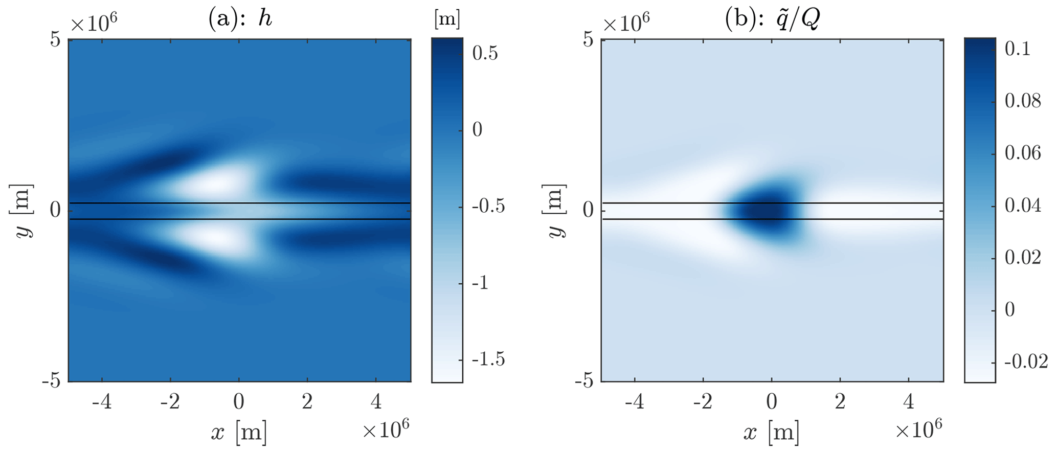
Figure 12 The thickness h (a) and perturbation moisture $q/Q$ (b) fields for a simulation of the system on an equatorial β plane, 400 d after initialisation from a state with a small-amplitude random q field, with $\mathit{\alpha }=\mathit{\lambda }={\mathrm{10}}^{-\mathrm{6}}{\mathrm{s}}^{-\mathrm{1}}$. The unstable region has been narrowed relative to the cases shown in Fig. 11 by decreasing the magnitude of the negative GMS at RCE. For this, we have set Q=10.5 m. The horizontal lines show y=y_stab. This disturbance propagates to the east at a speed of 0.15 m s⁻¹.

In contrast to the more complicated cases shown in Fig. 11a–e, the structures shown in Figs. 11f and 12 can be regarded as uniformly propagating, and the decomposition expressed by Eq. (40) can be usefully applied. Given that ϵ=0, it is exclusively the Q∇⋅u term that is of interest, and, as noted previously and using a method set out in Appendix D, this can be divided into the non-local quasi-steady Rossby and Kelvin wave responses to the heating F_h(q). The separate Rossby and Kelvin wave contributions to the propagation speed of equatorial moist regions for these two cases, calculated on the basis of Eq. (40) with the convergence term split into the two contributions, are shown in Fig. 13. Panels (a)–(b) are the cases originally shown in Fig. 11f, and panels (c)–(d) are the cases in Fig. 12.

As expected, the propagation direction does indeed depend on the relative strengths of the Kelvin wave response, which gives divergence to the east of the moisture anomaly and hence the heating anomaly, and the Rossby wave response, which gives divergence to the west, with, in both cases, corresponding convergence associated with the dry anomaly. Note that the patterns shown in Fig. 13 are made up of both the divergence associated with the moisture anomaly and the convergence associated with the dry anomaly. Panels (a)–(b) have a stronger equatorial Kelvin wave response, and hence the moist and dry regions travel westward, whereas in panels (c)–(d) the Rossby wave response is stronger, and eastward propagation is observed. In both cases the contributions from each of the wave types are of a similar magnitude, and there is significant cancellation. This has two implications: the propagation speeds will tend to be smaller than expected from a dynamical scaling argument, and the propagation speed and direction are sensitive to the latitudinal structure of the moisture, since the details of that structure determine the relative strength of the Kelvin and Rossby wave responses. Note that the mechanism described above that associates the Rossby wave response with eastward propagation is very different to mechanisms that are relevant to a similar association in other recent papers. The papers by Yano and Tribbia (2017) and Rostami and Zeitlin (2019) describe a strongly nonlinear Rossby wave that propagates eastward as a vortex pair, relying on nonlinearity in the vorticity and hence the momentum equations, which is absent in our model equations. The paper by Hayashi and Itoh (2017) describes a kind of diabatic Rossby wave, in which the vorticity field organises convective heating such that the resulting vorticity forcing implies propagation to the east. This mechanism is allowed in principle by our equations but is not consistent with the fact that the evolution as simulated can be explained by a quasi-steady dynamical balance.

Figure 13 The spatial structure (contours) of the Rossby (a, c) and Kelvin (b, d) wave responses to the moisture distribution (shading) of a uniformly propagating structure in two β-plane simulations. The contribution of each wave, estimated according to the method given in Appendix D, to the propagation speed is labelled. Panels (a)–(b) correspond to the state of the simulation in Fig. 11f, and panels (c)–(d) correspond to that shown in Fig. 12. Note that the colour bar in each panel has a different scale.

The arguments in Sect. 5.1 suggest that the parameter $c\mathit{\beta }/{\mathit{\alpha }}^{\mathrm{3}/\mathrm{2}}{\mathit{\lambda }}^{\mathrm{1}/\mathrm{2}}$ is important, with eastward propagation preferred when this is large. This is broadly consistent with the numerical simulations shown in Figs. 11 and 12, though this parameter certainly does not explain the propagation speed. For example, the system also shows a weak, complicated dependence of propagation speed and direction on diffusivity, with increasing κ both widening the boundaries between moist and dry regions and reducing y_stab. Regions which propagate to the east, seen in Fig. 11d and e, tend to have a spatial structure shaped like <. This structure, also noted in Sugiyama (2009b), may be explained by the same asymmetry of the Kelvin and Rossby responses that determine the direction of propagation. The Kelvin wave divergence to the east is necessarily localised near the Equator; however the Rossby wave response can be at any latitudinal scale. Hence, to the east of the moist region there is reduced moisture convergence near the Equator compared to further from the Equator; however to the west of the moist region there is reduced moisture convergence at all latitudes. There is therefore a tendency for off-equatorial (y>L_eq) regions of moisture to shift to the east. For a large moist region at the Equator extending into this region, an eastward tilt will be generated away from the Equator.

5.2.2  ϵ>0

A set of examples with ϵ=1 is shown in Fig. 14. The change in spatial structure of the moisture field from ϵ=0 to ϵ=1 is largely similar to that seen previously in the constant-f case (Fig. 6 versus Fig. 9). The associated convergence causes moist regions to narrow, and rotational flows at larger f lead to spirals in the moisture distribution.

Of the cases shown, (a), in Regime C, and (d), in Regime D, may be regarded as leading to a coherent steadily propagating disturbance (although the off-equatorial round regions in (a) are still unsteady). Panel (b) corresponds to Regime B and is closer to local quasi-isotropic aggregation, with features at different latitudes propagating at different speeds. This is highly unsteady, though the narrow propagation of the nonlinear advective convergence close to the Equator is preferentially in the zonal direction. Panel (c) resides near the boundary of Regimes B and C. The evolution is still very unsteady, with more evidence of rotational advection, particularly away from the Equator where f is non-zero.

Figure 14 Snapshots of the normalised perturbation moisture distribution $q/Q$ after 400 d of simulations with nonlinear dynamics (ϵ=1) on an equatorial β plane, with (a) $\mathit{\kappa }=\mathrm{4}\times {\mathrm{10}}^{\mathrm{5}}{\mathrm{m}}^{\mathrm{2}}{\mathrm{s}}^{-\mathrm{1}}$ and $\mathit{\alpha }=\mathit{\lambda }={\mathrm{10}}^{-\mathrm{5}}{\mathrm{s}}^{-\mathrm{1}}$, the same as Fig. 11f. Panel (b) has $\mathit{\kappa }={\mathrm{10}}^{\mathrm{5}}{\mathrm{m}}^{\mathrm{2}}{\mathrm{s}}^{-\mathrm{1}}$ and $\mathit{\alpha }=\mathit{\lambda }={\mathrm{10}}^{-\mathrm{5}}{\mathrm{s}}^{-\mathrm{1}}$, the same as Fig. 11a, and panel (c) has $\mathit{\kappa }={\mathrm{10}}^{\mathrm{5}}{\mathrm{m}}^{\mathrm{2}}{\mathrm{s}}^{-\mathrm{1}}$, $\mathit{\alpha }=\mathrm{3}\times {\mathrm{10}}^{-\mathrm{6}}{\mathrm{s}}^{-\mathrm{1}}$ and $\mathit{\lambda }=\mathrm{3}\times {\mathrm{10}}^{-\mathrm{5}}{\mathrm{s}}^{-\mathrm{1}}$ and does not correspond directly to a previous figure. Panel (d) illustrates the case with L_eq>y_stab and has the same parameters as Fig. 12. These reside in Regime C, Regime B, near the border of Regimes B and C, and Regime D respectively.

For the steadily propagating cases, the same technique as before, based on Eq. (40), can be used to decompose the different contributions to propagation as shown in Fig. 15. The nonlinear moisture advection term ϵ∇⋅(qu) is now present. It is helpful to separate the contribution from any zonal mean zonal flow. This is present because the segregation–aggregation process, with the form chosen for F_h(q) and F_q(q), tends to lead to a systematic zonal mean latitudinal structure in q, with greater q at low latitudes. This leads to a corresponding structure in h and hence in u. This zonal mean structure is present when ϵ=0 but then does not have any advective effect on q. The zonal mean u usually takes the form of two off-equatorial jets, centred where the latitudinal gradient in h is the largest. This zonal flow can potentially have a strong effect on propagation, but in the simulations shown here, the generation of a strong zonal flow is avoided by choosing λ to be sufficiently large so that variations in h are small. In practice, this means $\mathit{\lambda }=\mathcal{O}\left({\mathrm{10}}^{-\mathrm{5}}{\mathrm{s}}^{-\mathrm{1}}\right)$, well within the range discussed in the uniform rotation case.

Figure 15 The spatial structure (contours) of the (a) linear wave, (b) advection by the zonal mean flow $\stackrel{\mathrm{‾}}{u}$ and (c) nonlinear advection by the wave component contributions of the dynamical response to a moisture distribution (shading) of a propagating structure in a simulation on the β plane with nonlinear advection. This is the same case as shown in Fig. 14a. The contribution of each term to the propagation speed is labelled and has been calculated using Eq. (38).

For reference, the zonal mean u for the simulation in Fig. 15 is shown in Fig. 16. In this simulation the global mean u is 0.030 m s⁻¹. The damping still allows a non-zero zonal mean u; however this is significantly reduced. The domain mean u is constrained to be near zero to ensure that there is no advection by a uniform background flow.

Figure 16 The zonal mean velocity (a) and height (b) fields for the state of the nonlinear β-plane simulation shown in Fig. 15.

Returning to the decomposition into different contributions to propagation shown in Fig. 15, it may be seen that the linear divergence term (which has not been separated into Rossby and Kelvin contributions in this case, but the fact that the corresponding ΔU is positive implies that the Rossby contribution dominates), the term associated with advection by the zonal mean flow and the remaining nonlinear advection term are all comparable in magnitude.

6 Conclusions

In this study we have presented a single-layer model for convective aggregation and its connection to large-scale dynamics. The linearised shallow-water equations, governing the dynamics, are augmented with a moisture equation. The moisture field affects the dynamics via a heating term, i.e. a forcing term in the thickness equation, and the dynamics affects the moisture through convergence alone (ϵ=0) or with the additional effect of horizontal advection (ϵ>0). The forms of the moisture-dependent precipitation term and the moisture-dependent heating term are such that under the WTG approximation, the spatially homogeneous state, in which both precipitation and heating are zero (the RCE state), is unstable, and the system is bistable with moist and dry stable states (interpreted as convecting and non-convecting respectively). In this regime and with ϵ=0 the behaviour is described by a nonlinear reaction–diffusion equation for q, which is very similar to that presented by Craig and Mack (2013) and Windmiller and Craig (2019) (CMWC). As discussed by CMWC, the system exhibits a well-known spatial coarsening that may be interpreted as a representation of convective aggregation.

The difference between our model system and that in the CMWC case is that in the latter the form of the reaction term is determined solely through the dependence of precipitation on q. In our case it is determined in addition by the q-dependent heating, which couples to the moisture equation through the dynamics. This allows us to include more general dynamical effects beyond the WTG approximation, including the impact of thermal and frictional damping, nonlinear advection, and rotation, including the extension to the equatorial β plane. Under WTG dynamics with ϵ=0, the system, similar to the one studied by CMWC, coarsens to the largest available scale. This remains the case when nonlinear advection (ϵ>0) is included; however the coarsening process is modified, and the end state is different. Thermal and frictional damping and f-plane rotation in combination set a dynamical scale L_dyn, which is an upper limit on the validity of WTG. The result is that coarsening proceeds only to this scale and then ceases. Depending on the relative values of thermal and mechanical damping and rotation, the final state may essentially be steady, or it may be unsteady, with, in some cases, a symmetry breaking leading to loss of spatial isotropy and to propagating structures. The nature of the linearly unstable modes provides some guidance on the type of the final state that is observed. If f is large enough, with the critical value f_stab depending on moisture diffusivity κ as well as other parameters defining the system, then the RCE state is stable.

Many aspects of the behaviour of a β plane may be interpreted in terms of the previously discussed f-plane behaviour. A latitude y_stab may be defined by f_stab=βy_stab. Disturbances resulting from the instability of the RCE state are largely confined within the latitudinal band $(-y_{\mathrm{stab}},y_{\mathrm{stab}})$, with some penetration outside of this band as a result of the non-locality of the dynamics, typically with a scale of L_eq or the local value of L_dyn, whichever is the largest. When thermal and mechanical damping is strong enough, specifically when $c\mathit{\beta }{\mathit{\alpha }}^{-\mathrm{3}/\mathrm{2}}{\mathit{\lambda }}^{-\mathrm{1}/\mathrm{2}}<\mathrm{1}$, the evolution of the system is similar to that observed on the f plane, with spatial modulation corresponding to the spatial variation in the value of f. The weak anisotropy introduced by the β effect leads to zonal propagation. The propagation is incoherent, with structures at different latitudes propagating at different speeds; however those on the Equator propagate to the west. When $c\mathit{\beta }{\mathit{\alpha }}^{-\mathrm{3}/\mathrm{2}}{\mathit{\lambda }}^{-\mathrm{1}/\mathrm{2}}>\mathrm{1}$, the structures that form in the q field are more strongly anisotropic and coherently propagating, and it is helpful to formulate a description of the dynamics in terms of equatorial Kelvin and Rossby waves. If the former dominates the dynamical response to the q anomalies, there is propagation to the west; if the latter dominates, there is propagation to the east. Nonlinear moisture advection enhances eastward propagation, but the enhancement is not large. Whilst the model equations allow for time-dependent dynamics, the propagating disturbances that are seen in simulations can essentially be explained by considering the quasi-steady velocity fields forced by moisture-determined heating and consequently the effect of those velocity fields through convergence/divergence and nonlinear advection on the moisture field, indicating that these disturbances are moisture modes.

The β-plane results that we present, particularly for the $c\mathit{\beta }{\mathit{\alpha }}^{-\mathrm{3}/\mathrm{2}}{\mathit{\lambda }}^{-\mathrm{1}/\mathrm{2}}>\mathrm{1}$ regime, have significant common ground with those presented by Sugiyama (2009b). The behaviour observed in both studies is similar, with small-wavenumber and slowly propagating moist regions forming at the Equator. Indeed, as noted previously, one might argue that we are re-examining aspects of the models developed by Sugiyama (2009a, b). These models include WISHE, which we do not, and have a physically derived formulation of the forcing terms F_q and F_h, which in some circumstances leads to bistability (Sugiyama, 2009a). We, on the other hand, emphasise the general implications of the bistability of the system, motivated by various lines of investigation, such as single-column radiative–convective calculations in WTG models (e.g. Sobel et al., 2007; Emanuel et al., 2014), and then choose very simple ad hoc forms of F_q(q) and F_h(q) to provide such bistability. We also deliberately trace the behaviour of the system through a sequence starting with WTG dynamics, and hence the reaction–diffusion behaviour discussed by CMWC, and finishing with the β plane with thermal and mechanical damping and nonlinear moisture advection that was the focus of Sugiyama (2009b), thereby providing a new perspective on the latter.

One difference between the conclusions of this study and those of Sugiyama (2009b) is that the latter suggests that diffusion is an important contributor to the eastward propagation of moist regions in the nonlinear advection case. We, however, conclude that the propagation is due to a combination of nonlinear advection and the displaced convergence associated with the Rossby wave response. This difference in interpretation arises in part from the diagnostic approaches used to measure the impact of different terms of the moisture tendency. We assume a uniformly propagating disturbance and then calculate a contribution from each moisture tendency term to the speed of propagation using Eq. (40), taking into account the entire spatial distribution. As noted previously, according to this approach the net contribution of the diffusive term to propagation is zero, whereas Sugiyama (2009b) compares the tendencies at y=0. Only comparing at y=0 will overestimate the contribution of the diffusive tendency to the overall propagation. In an aggregated region shaped like <, the negative curvature at the Equator to the east increases the diffusive speed of the boundary, whereas the opposite is true away from the Equator where the sign of the curvature changes. The fact that according to Eq. (15) the net contribution of diffusion to propagation is identically zero does not, of course, rule out the possibility that the form of the terms that do contribute to net propagation are affected by diffusivity. Certainly, there is evidence of diffusivity dependence of propagation speed in the results presented, for example in cases (a) and (f) in Fig. 11, where increasing diffusivity increases westward propagation speed, and cases (a) and (b) in Fig. 14, where increasing diffusivity increases eastward propagation speed. A further difference from Sugiyama (2009b) is that we have not assumed h dependence in F_h and F_q. As has been noted previously, this follows other moisture-mode models, including Sobel and Maloney (2012, 2013) and Adames and Kim (2016), but a preliminary assessment of the effect of including h dependence is given in Appendix E and concludes that the formation, evolution and propagation of moist and dry regions, as described in Sect. 5 above, remain broadly unchanged when this is included.

Recent review articles on convective aggregation, for example Wing et al. (2017) and Muller et al. (2022), include the CMWC reaction–diffusion model in their discussion of different mechanisms and models. The model we have presented above generalises CMWC by linking the moisture and large-scale dynamical equations. In the categorisation given by Wing et al. (2017), our model fits the category of a long-wave radiation feedback with an additional advective process feedback included if ϵ>0. The CMWC model, on the other hand, which relies on the form of the moisture dependence of precipitation, is categorised as a moisture feedback. Unlike the CMWC model, our model, by including dynamics, provides an upper limit on the scale of the aggregation scale, which is finite and determined by thermal and momentum damping rates when f=0 and reduces as f increases. How this relates to evidence from GCM and CRM simulations remains to be determined, although recent CRM studies show the potential for multiple aggregated regions in larger domains and more complex structures with a characteristic length scale (Yanase et al., 2022; Patrizio and Randall, 2019).

Whilst most high-resolution three-dimensional modelling of convective aggregation has focused on the non-rotating case, there has been some recent investigation of the f-plane and β-plane cases (Carstens and Wing, 2022, 2023). Some aspects of the behaviour reported in those papers are seen in our much simpler model. On the f plane, circular moist (i.e. convecting) regions form, and the scale of these regions decreases as f increases, scaling as $\mathrm{1}/f$ in both models at large rotation rates. However the physics of this behaviour is likely to be very different between the two models. In the CRM studies of Carstens and Wing (2022), the structure for larger values of f is dominated by tropical cyclones. These features have no clear analogue in our model, which neglects advective nonlinearity in the momentum equation. Carstens and Wing (2022) identify an intermediate range of f within which convective aggregation simply does not occur. One possibility is that this corresponds to our f>f_stab, with formation of tropical cyclones being a distinct process that occurs at a larger f value in the CRM but which is simply absent in our model. On the β plane, Carstens and Wing (2023) identify the dominant structures that arise from convective aggregation at low latitudes as convectively coupled Kelvin waves, whereas in our model the structures are clearly characteristic of moisture modes, with quasi-steady dynamical fields. In future work it would be interesting to investigate further whether there are parameter regimes in which our model also shows moisture-modified Kelvin waves as the dominant low-latitude structures.

One goal of formulating and studying the model presented in this paper was to provide a basis for understanding the MJO. But in several respects, with the model in its current form, this goal has not been met. One aspect of this is the phenomenon of aggregation, which might have provided an explanation for the large longitudinal scale of the MJO without requiring a scale-selection mechanism for an underlying instability, such as radiative–convective instability, which is consistent with such a large scale. However the rate of increase in scale due to aggregation is in our model determined by diffusivity of moisture and, with the value assumed, $\mathit{\kappa }={\mathrm{10}}^{\mathrm{5}}{\mathrm{m}}^{\mathrm{2}}{\mathrm{s}}^{-\mathrm{1}}$, the time taken to reach scales of thousands of kilometres is (at least) many tens of days. This does not seem consistent with the observed MJO evolution in which convection appears to develop over a large, perhaps 10⁴ km region of the Indian Ocean on a timescale of a few days. A larger value of diffusivity would reduce the time required but might be difficult to justify – e.g. see the arguments in Biagioli and Tompkins (2023). It might be that aggregation acts alongside large-scale-selective processes such as the radiative destabilisation suggested by Adames and Kim (2016).

A second aspect is the horizontal structure and propagation characteristics of disturbances predicted by the model on an equatorial β plane. Our model in this form is similar to that considered previously by Sugiyama (2009b), and our conclusions are also similar. There is organisation into distinct moist and dry regions on the Equator, and these propagate in the zonal direction. Similar to Sugiyama (2009b), we emphasise that these propagating disturbances are fundamentally nonlinear, and their structure and propagation characteristics are not captured by a linear stability analysis. However, the direction of propagation can be westward or eastward, and the speed of propagation is consistently much less than 1 m s⁻¹ when the observed MJO phase speed is around 5 m s⁻¹. Furthermore, even when the propagation is eastward-propagating disturbances, the spatial structure of eastward-propagating moist regions also necessarily forms a < shape compared to the > structure of the observed MJO (Adames and Wallace, 2014).

It seems likely that, for a model of this nonlinear moisture-mode form to produce more realistic MJO-like behaviour, further physics needs to be included (though it should not be forgotten that MJO-like behaviour can also be produced by models with a different form). Recent simple one-dimensional moisture-mode models for the MJO (Sobel and Maloney, 2013; Adames and Kim, 2016), which are based on a prescribed latitudinal structure of the flow variables, have included extra effects, such as synoptic eddy drying, boundary-layer convergence of moisture (Adames and Wallace, 2014) and latitudinal gradients in background moisture (Adames and Kim, 2016), and have shown that these effects lead to enhanced eastward propagation. However the results we have presented in Sect. 5 of this paper demonstrate that propagation speed and direction are sensitive to latitudinal structure, so there are disadvantages to prescribing this a priori. We currently include some of these effects in the two-dimensional model described in this paper with the aim of capturing the behaviour of nonlinear MJO-like disturbances in a model where the two-dimensional structure emerges rather than being prescribed. Such a model could also potentially be used to study a broader class of moist tropical variability (e.g. Wang and Sobel, 2022).

Appendix A: Numerical details

To solve Eqs. (1)–(3) numerically, we use standard methods for solving the shallow-water equations. The equations are discretised on an Arakawa C grid with the grid spacing chosen to be $d=\mathrm{4}\times {\mathrm{10}}^{\mathrm{4}}\mathrm{m}$. The system is then numerically stepped forward in time using a third-order Adams–Bashforth scheme with a time step of 112.5 s.

On the f plane, we take (doubly) periodic boundaries, whereas on the equatorial β plane, rigid north and south boundaries are used along with periodic east and west boundaries. At rigid boundaries, a sponge layer is included to avoid edge effects. This takes the form of a linear damping term included in the velocity and thickness fields. On the periodic channel we use on the β plane this takes the following form:

$$\begin{array}{}\text{(A1)}& \begin{array}{rl}{\mathit{\alpha }}_{\mathrm{sponge}}& =\mathrm{1}\times {\mathrm{10}}^{-\mathrm{5}}\left[\exp \left(-{\displaystyle \frac{\mathrm{70}(L_y-\mathrm{2}y)}{L_y}}\right)\right.\\ & \left.+\exp \left({\displaystyle \frac{\mathrm{70}(L_y+\mathrm{2}y)}{L_y}}\right)\right]{\mathrm{s}}^{-\mathrm{1}}.\end{array}\end{array}$$

The magnitude decays over a scale of $\mathrm{1}/\mathrm{70}$th of the domain. Any numerical results discussed in this paper do not depend on the magnitude or decay scale of this damping term.

Appendix B: Details of the f-plane linear stability problem

This appendix gives further details of the linear stability problem considered in Sect. 4.1. Considering small-amplitude perturbations of the form $u=\mathrm{\Re }\mathit{\left\{}\widehat{u}\exp \right(\mathit{\sigma }t+ikx\left)\mathit{\right\}}$, with analogous notation for other variables, the linearised forms of Eqs. (1), (2) and (3) lead to (14), (15), (16) and (17), with ${\mathit{\mu }}_{\mathrm{2}}=-F_h^{\prime }\left(\mathrm{0}\right)$ and ${\mathit{\mu }}_{\mathrm{1}}=-F_q^{\prime }\left(\mathrm{0}\right)$, matching the notation used in Eqs. (13) and (12) respectively. These define an eigenvalue problem for the growth rate σ, which is a root of the quartic equation

$$\begin{array}{}\text{(B1)}& \begin{array}{rl}& {\mathit{\sigma }}^{\mathrm{4}}+[\mathit{\lambda }+\mathrm{2}\mathit{\alpha }+{\mathit{\mu }}_{\mathrm{1}}+\mathit{\kappa }{k}^{\mathrm{2}}]{\mathit{\sigma }}^{\mathrm{3}}\\ & +\left[\right({\mathit{\mu }}_{\mathrm{1}}+\mathit{\kappa }{k}^{\mathrm{2}}\left)\right(\mathit{\lambda }+\mathrm{2}\mathit{\alpha })+f^{\mathrm{2}}+c^{\mathrm{2}}{k}^{\mathrm{2}}+{\mathit{\alpha }}^{\mathrm{2}}+\mathrm{2}\mathit{\alpha }\mathit{\lambda }]{\mathit{\sigma }}^{\mathrm{2}}\\ & +\left[\right({\mathit{\mu }}_{\mathrm{1}}+\mathit{\kappa }{k}^{\mathrm{2}}\left)\right(f^{\mathrm{2}}+c^{\mathrm{2}}{k}^{\mathrm{2}}+{\mathit{\alpha }}^{\mathrm{2}}+\mathrm{2}\mathit{\alpha }\mathit{\lambda })+c^{\mathrm{2}}{k}^{\mathrm{2}}\mathit{\alpha }\\ & +(f^{\mathrm{2}}+{\mathit{\alpha }}^{\mathrm{2}})\mathit{\lambda }-g{\mathit{\mu }}_{\mathrm{2}}Q{k}^{\mathrm{2}}]\mathit{\sigma }\\ & +({\mathit{\mu }}_{\mathrm{1}}+\mathit{\kappa }{k}^{\mathrm{2}})c^{\mathrm{2}}{k}^{\mathrm{2}}\mathit{\alpha }-g{\mathit{\mu }}_{\mathrm{2}}Q{k}^{\mathrm{2}}\mathit{\alpha }\\ & +(f^{\mathrm{2}}+{\mathit{\alpha }}^{\mathrm{2}})\mathit{\lambda }({\mathit{\mu }}_{\mathrm{1}}+\mathit{\kappa }{k}^{\mathrm{2}})=\mathrm{0},\end{array}\end{array}$$

with coefficients that are either linear or quadratic in k². Simple limits of the above in the case where $f=\mathit{\alpha }=\mathit{\lambda }=\mathrm{0}$ have been noted previously, in particular in the WTG limit valid at small scales such that $k\gg \mathit{\mu }/c$ and the corresponding large-scale results for $k\ll \mathit{\mu }/c$.

To further analyse the behaviour of the full system as described by Eq. (B1), we first consider the case where α and λ are non-zero, but there is no rotation; i.e. f=0. It is helpful to note the solutions for σ in the large-scale (k small) and small-scale (k large) limits. Neglecting diffusion, it is straightforward to show that at small k the roots of Eq. (B1) are $\mathit{\sigma }\simeq -\mathit{\lambda },-\mathit{\alpha },-\mathit{\alpha }$ and −μ₁ (i.e. the $\mathit{\sigma }\simeq -\mathit{\alpha }$ root is repeated in the limit as k→0), implying stability at small k. Correspondingly, at large k there are roots $\mathit{\sigma }\simeq \pm ick-\mathit{\lambda }-{\mathit{\mu }}_{\mathrm{2}}Q/H,-\mathit{\alpha },{\mathit{\mu }}_{\mathrm{2}}(Q/H)-{\mathit{\mu }}_{\mathrm{1}}=-{\mathit{\mu }}_{\mathrm{1}}M$, representing two gravity waves damped by moisture effects and thermal damping, a vorticity disturbance damped by friction, and a moisture mode (stable or unstable according to whether M is positive or negative) respectively. There is therefore stability at small k and, consistent with the WTG analysis, instability at large k if M>0, with the latter limit unaffected by α and λ being non-zero. Introducing diffusion by taking κ>0 will lead to all roots having negative real parts as k→∞; i.e. the system is stabilised by diffusion of moisture.

Given that all roots for σ have negative real parts for k→0, it is possible to deduce whether or not there is instability by seeking conditions, in particular a value of k, under which one of the roots has zero real parts. One possibility is σ=is, where s is real and non-zero. Substituting this form for σ into Eq. (B1), with f=0, shows that such a root is not possible. (A key simplification in the f=0 case that can be exploited here is that the fourth-order polynomial appearing in Eq. (B1) has a factor (σ+α).) The other possibility is that σ=0, implying the condition

$$\begin{array}{}\text{(B2)}& ({\mathit{\mu }}_{\mathrm{1}}+\mathit{\kappa }{k}^{\mathrm{2}})c^{\mathrm{2}}{k}^{\mathrm{2}}\mathit{\alpha }-g{\mathit{\mu }}_{\mathrm{2}}Q{k}^{\mathrm{2}}\mathit{\alpha }+{\mathit{\alpha }}^{\mathrm{2}}\mathit{\lambda }({\mathit{\mu }}_{\mathrm{1}}+\mathit{\kappa }{k}^{\mathrm{2}})=\mathrm{0}.\end{array}$$

This is a quadratic for k², which has real roots only if

$$\begin{array}{}\text{(B3)}& \mathit{\kappa }\le {\displaystyle \frac{c^{\mathrm{2}}{\mathit{\mu }}_{\mathrm{1}}}{\mathit{\lambda }\mathit{\alpha }}}(\sqrt{\mathrm{1}-M}-\mathrm{1}{)}^{\mathrm{2}},\end{array}$$

where, as before, $M=\mathrm{1}-{\mathit{\mu }}_{\mathrm{2}}Q/{\mathit{\mu }}_{\mathrm{1}}H$. If this condition is satisfied, then there is instability. If it is not satisfied, then there is no instability. Furthermore, it may also be deduced that roots with positive real parts must be real and that for any value of k there can be at most one such root. Given that roots crossing the real axis must do so at σ=0, complex roots with positive real parts would be possible only if there were two such crossings, from below to above the real axis, as k increased, and those real roots then combined to give a complex conjugate pair. But this is not possible since the above shows that there are at most two crossings for any k, and, given that all roots are below the real axis for small k and (with κ>0) for large k, one crossing is from below the real axis to above, and the other is from above to below.

When f is non-zero the conditions for instability are more complicated. The large-k limits of the roots of Eq. (B1) are unaffected by the expressions given above (which were for κ=0; the same holds for κ>0). However the small-k limits are now $\mathit{\sigma }\simeq -\mathit{\lambda },\pm if-\mathit{\alpha },-{\mathit{\mu }}_{\mathrm{1}}$, implying stability at small k, but note that the previously repeated root −α now becomes the complex conjugate pair $\pm if-\mathit{\alpha }$ (i.e. frictionally damped inertial oscillations). The transition between small k and large k now depends on the values of α, λ, f, κ and other parameters. The expression (Eq. B3) for real roots of Eq. (B1) to cross the real axis generalises to (repeating Eq. 21)

$$\begin{array}{}\text{(B4)}& \mathit{\kappa }\le {\displaystyle \frac{c^{\mathrm{2}}{\mathit{\mu }}_{\mathrm{1}}\mathit{\alpha }}{\mathit{\lambda }({\mathit{\alpha }}^{\mathrm{2}}+f^{\mathrm{2}})}}(\sqrt{\mathrm{1}-M}-\mathrm{1}{)}^{\mathrm{2}};\end{array}$$

however this does not give complete information on when instability is possible because with f non-zero complex conjugate roots may also cross the real axis. Some analytical progress can be made in describing the dependence of roots on the different parameters, but the algebra is complicated.

As described in Sect. 4.1, numerical investigation shows that, for a given κ, the (α,λ) plane may be divided into four regions, each corresponding to a different regime of behaviour. Regime I is where ℜ(σ)>0 occurs for some k only when σ is real. Regimes IIa and IIb are where there are complex σ with ℜ(σ)>0 and with non-zero imaginary parts, and Regime III is where there is no instability, i.e. ℜ(σ)<0 for all k. The distinction between IIa and IIb is that in IIb, σ corresponding to the fastest growth over all k has a non-zero imaginary part. (An example is given in Fig. 5.) For f=0 only Regimes I and III are present, and Regime I, the region of instability, simply corresponds to Eq. (B3).

The boundary between Regime I and Regime IIa, indicated by the dashed curves in Fig. 5, is predicted by the condition that Eq. (B1) has a double root at σ=0. This is because close to the λ=0 axis a real root crosses the real axis. As λ increases, a bifurcation point emerges on the solution branch, joining to that root, and then moves towards the real axis. A transition between the crossing of the real axis by a real root and the crossing by a complex conjugate pair occurs when the bifurcation point reaches the real axis, i.e. at the point where there is a double root at σ=0. For all f such that Regimes IIa and IIb exist, the boundary between Regime IIa and Regime I asymptotes to α≃λ as λ→0. The condition for a double root at σ=0 must be compatible with the condition given by Eq. (B4). Given that the gradient of the dashed curves is observed to reduce as λ increases, there will not be compatibility if the gradient of the curve defined by equality in Eq. (B4) is larger than 1 as λ→0, i.e. if

$$\begin{array}{}\text{(B5)}& f>c({\mathit{\mu }}_{\mathrm{1}}/\mathit{\kappa }{)}^{\mathrm{1}/\mathrm{2}}(\sqrt{\mathrm{1}-M}-\mathrm{1}).\end{array}$$

When this inequality is satisfied there are no Regimes IIa and IIb, and the transition between stability and instability is fully described by Eq. (B4) or, equivalently, Eq. (21). The double root at σ=0 occurs when both the constant term and the coefficient of the linear term in Eq. (B1) vanish simultaneously. Eliminating k² gives a constraint on λ and α (for given values of other parameters such as f and κ), which defines the boundary between regions I and IIa in Fig. 5. For illustrative purposes, the resulting expression when κ=0 is

$$\begin{array}{}\text{(B6)}& \begin{array}{rl}& \mathit{\lambda }={\mathit{\lambda }}_{*}\left(\mathit{\alpha }\right)\\ & ={\displaystyle \frac{({\mathit{\alpha }}^{\mathrm{2}}+f^{\mathrm{2}})(Q{\mathit{\mu }}_{\mathrm{2}}/H-{\mathit{\mu }}_{\mathrm{1}}){\mathit{\mu }}_{\mathrm{1}}\mathit{\alpha }}{(Q{\mathit{\mu }}_{\mathrm{2}}/H-{\mathit{\mu }}_{\mathrm{1}})(f^{\mathrm{2}}{\mathit{\mu }}_{\mathrm{1}}-f^{\mathrm{2}}\mathit{\alpha }-{\mathit{\alpha }}^{\mathrm{2}}{\mathit{\mu }}_{\mathrm{1}}-{\mathit{\alpha }}^{\mathrm{3}})-\mathit{\alpha }{\mathit{\mu }}_{\mathrm{1}}(f^{\mathrm{2}}+{\mathit{\alpha }}^{\mathrm{2}})}}.\end{array}\end{array}$$

In the small-α limit it corresponds to λ≃α. Since this expression for λ_*(α) ignores diffusivity, it will provide an accurate description of the boundary between regions I and IIa only when it is approximately independent of diffusivity, which, as seen in Fig. 5, appears to be the case when λ and α are small.

The boundary between regions IIb and III corresponds to a double root of Eq. (B1) of the form σ=is, s≠0. Some information about the small-α part of this boundary can be obtained by considering the special case α=0. There is then a root that is 𝒪(k²) for small k, with a real part that has the same sign as $\mathit{\lambda }{\mathit{\mu }}_{\mathrm{1}}\left({\mathit{\mu }}_{\mathrm{2}}\right(Q/H)-{\mathit{\mu }}_{\mathrm{1}})-f^{\mathrm{2}}(\mathit{\lambda }+{\mathit{\mu }}_{\mathrm{2}}(Q/H\left)\right)$. It follows that for $f^{\mathrm{2}}<\left({\mathit{\mu }}_{\mathrm{2}}\right(Q/H)-{\mathit{\mu }}_{\mathrm{1}}){\mathit{\mu }}_{\mathrm{1}}$ there is instability at small k for large λ; therefore stabilisation requires non-zero α. On the other hand, for $f^{\mathrm{2}}>\left({\mathit{\mu }}_{\mathrm{2}}\right(Q/H)-{\mathit{\mu }}_{\mathrm{1}}){\mathit{\mu }}_{\mathrm{1}}$ there is stability at large λ, independent of the value of α. This explains the different forms of the boundary between regions IIb and III seen in Fig. 5 for f=0 and $f={\mathrm{10}}^{-\mathrm{5}}$s⁻¹ on the one hand and $f=\mathrm{3}\times {\mathrm{10}}^{-\mathrm{5}}$ s⁻¹ and $f=\mathrm{6}\times {\mathrm{10}}^{-\mathrm{5}}$ s⁻¹ on the other.

The condition $f=f_{\mathrm{stab}}(\mathit{\lambda },\mathit{\alpha })$ defines a function on the (λ,α) plane as the maximum f for a given α and λ (with dependence on other parameters such as κ suppressed) for which there are unstable modes. Contours of this function are shown in Fig. 5 as the bounding curves for Regime III.

It can be seen from Fig. 5 that the variation in $f=f_{\mathrm{stab}}(\mathit{\lambda },\mathit{\alpha })$ is non-smooth and that this continues into the region of the (λ,α) plane where α and λ are both small, implying that the limiting value of f_stab(α,λ) as α→0 and λ→0 cannot be straightforwardly defined. To analyse this regime further it is useful to set $\mathit{\alpha }=\mathit{\lambda }=\mathrm{0}$ in Eq. (B1), leading to

$$\begin{array}{}\text{(B7)}& \begin{array}{rl}{\mathit{\sigma }}^{\mathrm{3}}& +\left(\mathit{\kappa }{k}^{\mathrm{2}}+{\mathit{\mu }}_{\mathrm{1}}\right){\mathit{\sigma }}^{\mathrm{2}}+\left(f^{\mathrm{2}}+c^{\mathrm{2}}{k}^{\mathrm{2}}\right)\mathit{\sigma }+f^{\mathrm{2}}{\mathit{\mu }}_{\mathrm{1}}+c^{\mathrm{2}}\mathit{\kappa }{k}^{\mathrm{4}}\\ & +f^{\mathrm{2}}\mathit{\kappa }{k}^{\mathrm{2}}+c_m^{\mathrm{2}}{k}^{\mathrm{2}}{\mathit{\mu }}_{\mathrm{1}}=\mathrm{0},\end{array}\end{array}$$

where the moist gravity wave speed is $c_m^{\mathrm{2}}=c^{\mathrm{2}}M<\mathrm{0}$ for the potentially unstable case. The roots of this polynomial are denoted as σ₁, σ₂ and σ₃.

First, assume that there is a purely imaginary root σ=is, where s is real. Substituting into Eq. (B7) and separating the real and imaginary parts give

$$\begin{array}{}\text{(B8)}& {\displaystyle }{s}^{\mathrm{3}}=(f^{\mathrm{2}}+c^{\mathrm{2}}{k}^{\mathrm{2}})s,\text{(B9)}& {\displaystyle }({\mathit{\mu }}_{\mathrm{1}}+\mathit{\kappa }{k}^{\mathrm{2}})s^{\mathrm{2}}={\mathit{\mu }}_{\mathrm{1}}{f}^{\mathrm{2}}+{\mathit{\mu }}_{\mathrm{1}}{c}_m^{\mathrm{2}}{k}^{\mathrm{2}}+f^{\mathrm{2}}\mathit{\kappa }{k}^{\mathrm{2}}+c^{\mathrm{2}}\mathit{\kappa }{k}^{\mathrm{4}}.\end{array}$$

Eliminating s gives

$$\begin{array}{}\text{(B10)}& ({\mathit{\mu }}_{\mathrm{1}}+\mathit{\kappa }{k}^{\mathrm{2}})(f^{\mathrm{2}}+c^{\mathrm{2}}{k}^{\mathrm{2}})={\mathit{\mu }}_{\mathrm{1}}{f}^{\mathrm{2}}+{\mathit{\mu }}_{\mathrm{1}}{c}_m^{\mathrm{2}}{k}^{\mathrm{2}}+f^{\mathrm{2}}\mathit{\kappa }{k}^{\mathrm{2}}+c^{\mathrm{2}}\mathit{\kappa }{k}^{\mathrm{4}}.\end{array}$$

For k>0, this is true only in the dry case $c_m^{\mathrm{2}}=c^{\mathrm{2}}$. Since we are interested in $c_m^{\mathrm{2}}<\mathrm{0}<c^{\mathrm{2}}$, purely imaginary roots are not possible. Therefore any change in stability happens at σ=0.

For small k, Eq. (B7) has roots $\mathit{\sigma }=-{\mathit{\mu }}_{\mathrm{1}}$ and $\mathit{\sigma }=\pm if-k^{\mathrm{2}}(\mathrm{2}g{\mathit{\mu }}_{\mathrm{2}}{\mathit{\mu }}_{\mathrm{1}}{f}^{\mathrm{2}}Q\pm \mathrm{2}if(f^{\mathrm{2}}{c}^{\mathrm{2}}+c_m^{\mathrm{2}}{\mathit{\mu }}_{\mathrm{1}}^{\mathrm{2}}\left)\right)/\mathrm{4}(f^{\mathrm{4}}+f^{\mathrm{2}}{\mathit{\mu }}_{\mathrm{1}}^{\mathrm{2}})$, both of which have negative real parts. For instability, a change in stability must occur at some k>0. This requires the constant coefficient of Eq. (B7) to change sign; i.e.

$$\begin{array}{}\text{(B11)}& {\mathit{\mu }}_{\mathrm{1}}{f}^{\mathrm{2}}+{\mathit{\mu }}_{\mathrm{1}}{c}_m^{\mathrm{2}}{k}^{\mathrm{2}}+f^{\mathrm{2}}\mathit{\kappa }{k}^{\mathrm{2}}+c^{\mathrm{2}}\mathit{\kappa }{k}^{\mathrm{4}}=\mathrm{0}.\end{array}$$

If the system is to be stable, this must have no real roots k²>0. We non-dimensionalise with $\widehat{f}=f\sqrt{\mathit{\kappa }/{\mathit{\mu }}_{\mathrm{1}}}/c$ and $\widehat{k}=k/\sqrt{\mathit{\kappa }/{\mathit{\mu }}_{\mathrm{1}}}$, for

$$\begin{array}{}\text{(B12)}& {\widehat{f}}^{\mathrm{2}}+M{\widehat{k}}^{\mathrm{2}}+{\widehat{f}}^{\mathrm{2}}{\widehat{k}}^{\mathrm{2}}+{\widehat{k}}^{\mathrm{4}}=\mathrm{0}.\end{array}$$

The transition from two roots to none happens when the discriminant of this expression (as a quadratic in k) vanishes, or

$$\begin{array}{}\text{(B13)}& (M+\widehat{f}{)}^{\mathrm{2}}-\mathrm{4}{\widehat{f}}^{\mathrm{2}}=\mathrm{0}.\end{array}$$

This has four roots,

$$\begin{array}{}\text{(B14)}& \widehat{f}=\pm (\mathrm{1}-\sqrt{\mathrm{1}-M}),\end{array}$$

corresponding to the change in global stability, and

$$\begin{array}{}\text{(B15)}& \widehat{f}=\pm (\mathrm{1}+\sqrt{\mathrm{1}-M}),\end{array}$$

which is a spurious solution arising from roots with k²<0. (When ${\widehat{f}}^{\mathrm{2}}>\mathrm{1}-M$, the left-hand side of Eq. (B12) is strictly positive for k²>0.)

With zero damping, and assuming positive f, we therefore expect instability if and only if

$$\begin{array}{}\text{(B16)}& f<={\displaystyle \frac{c}{\sqrt{\mathit{\kappa }/{\mathit{\mu }}_{\mathrm{1}}}}}(\sqrt{\mathrm{1}-M}-\mathrm{1})=f_{\mathrm{stab}}(\mathrm{0},\mathrm{0}),\end{array}$$

where the value of f_stab(0,0) is defined by this equality. Since only one mode may be unstable in this limiting case, the unstable mode must have a purely real growth rate. When the function f_stab(α,λ) is defined by Eq. (B4), the limit of this expression as α→0 and λ→0 is not well defined, since it depends on the value of $\mathit{\alpha }/\mathit{\lambda }$.

This inconsistency may be resolved as follows. There is a value f_I such that the region of the (λ,α) space defined by $f_{\mathrm{stab}}(\mathit{\lambda },\mathit{\alpha })>f_I$ contains no parameters corresponding to Regime II; i.e. the unstable roots of Eq. (B1) are real for all k. Within this region, the stability boundary is given by Eq. (B4), rewritten here as a curve in the (λ,α) plane,

$$\begin{array}{}\text{(B17)}& \mathit{\lambda }={\displaystyle \frac{c^{\mathrm{2}}{\mathit{\mu }}_{\mathrm{1}}\mathit{\alpha }}{\mathit{\kappa }({\mathit{\alpha }}^{\mathrm{2}}+f^{\mathrm{2}})}}(\sqrt{{\mathit{\mu }}_{\mathrm{2}}Q/{\mathit{\mu }}_{\mathrm{1}}H}-\mathrm{1}{)}^{\mathrm{2}}.\end{array}$$

Note that as f is made arbitrarily large, this curve moves closer to the α axis, but does not meet it, so there is always some range of α such that there is instability for λ=0. Within this region, the transition with varying k of a single real mode from unstable to stable corresponds to the change in sign of the constant term of Eq. (B1). When $\mathit{\alpha }=\mathit{\lambda }=\mathrm{0}$, this constant term is identically zero. We therefore have a degenerate case where the previously unstable mode is zero for all k. The limit as α→0 and λ→0 of f_stab in this region is therefore not expected to be well defined.

In the other section of the (λ,α) plane, where f_stab<f_I, instability both near the origin and near f=f_stab relies on a combination of two complex roots of Eq. (B1). If α→0 and λ→0, only one of these roots can become identically zero, so we expect the other to remain the unstable mode, and hence the limit of f_stab should be well defined.

Since f_stab is continuous (apart from at the origin), we also expect the limit along the boundary between each of the cases discussed above, f_stab=f_I, to give the correct value of f_stab(0,0). This is a curve of constant f_stab, and therefore

$$\begin{array}{}\text{(B18)}& f_I=f_{\mathrm{stab}}(\mathrm{0},\mathrm{0})={\left({\displaystyle \frac{c^{\mathrm{2}}(\sqrt{{\mathit{\mu }}_{\mathrm{2}}Q/{\mathit{\mu }}_{\mathrm{1}}H}-\mathrm{1}{)}^{\mathrm{2}}}{\mathit{\kappa }/{\mathit{\mu }}_{\mathrm{1}}}}\right)}^{\mathrm{1}/\mathrm{2}}.\end{array}$$

The curve $f_{\mathrm{stab}}(\mathit{\lambda },\mathit{\alpha })=f_{\mathrm{stab}}(\mathrm{0},\mathrm{0})$ has the expected form, α=λ, when α≪f.

Appendix C: The equatorial wave response to a moist heating

The full derivation of linear equatorial wave response to a heating with general thermal damping λ and friction α is derived by Wu et al. (2001). The setup and relevant results are repeated here for reference.

We look for equatorially trapped steady-state solutions to the dynamical Eqs. (1) and (3), under the long-wave approximation. These satisfy

$$\begin{array}{}\text{(C1)}& {\displaystyle }\mathit{\alpha }u-\mathit{\beta }yv=-g{h}_x,\text{(C2)}& {\displaystyle }\mathit{\beta }yu=-g{h}_y,\text{(C3)}& {\displaystyle }\mathit{\lambda }h+H\mathrm{\nabla }\cdot \mathit{u}=F,\end{array}$$

where u, v and h→0 are $y\to \pm \mathrm{\infty }$. For simplicity, we take a domain of effectively infinite zonal length, i.e. with a length much greater than the extent of the equatorial wave response. We can also assume that F(x,y) has a mean of zero, as a non-zero spatial mean part will be balanced by a change in the mean h and not contribute to the divergence or equatorial wave response.

We must first decompose the heating in terms of parabolic cylinder functions ${\stackrel{\mathrm{̃}}{D}}_n$ as

$$\begin{array}{}\text{(C4)}& F=\sum _{n\ge \mathrm{0}}{F}_n{\stackrel{\mathrm{̃}}{D}}_n\left({\displaystyle \frac{y}{L_{\mathrm{eq}}}}\right),\end{array}$$

with $L_{\mathrm{eq}}=\sqrt{c/\mathit{\beta }}\sqrt[\mathrm{4}]{\mathit{\alpha }/\mathit{\lambda }}$.

The relevant parts of the solutions are then the equatorial Kelvin wave, which has

$$\begin{array}{}\text{(C5)}& \begin{array}{rl}{h}_{\mathrm{0}}& =-{\displaystyle \frac{\mathrm{1}}{\mathrm{2}}}\underset{-\mathrm{\infty }}{\overset{x}{\int }}\sqrt{{\displaystyle \frac{\mathit{\alpha }}{\mathit{\lambda }}}}{c}^{-\mathrm{1}}\exp \left(-{\displaystyle \frac{\sqrt{\mathit{\alpha }\mathit{\lambda }}(x-u)}{c}}\right)\\ & F_{\mathrm{0}}\left(u\right)\mathrm{d}u{\stackrel{\mathrm{̃}}{D}}_{\mathrm{0}}\left({\displaystyle \frac{y}{L_{\mathrm{eq}}}}\right),\end{array}\end{array}$$

and the equatorial Rossby waves, for $n=\mathrm{1},\mathrm{2},\mathrm{3},\mathrm{\dots }$,

$$\begin{array}{}\text{(C6)}& \begin{array}{rl}{h}_n& =-{\displaystyle \frac{\mathrm{1}}{\mathrm{2}}}\underset{x}{\overset{\mathrm{\infty }}{\int }}\sqrt{{\displaystyle \frac{\mathit{\alpha }}{\mathit{\lambda }}}}{c}^{-\mathrm{1}}\exp \left({\displaystyle \frac{(\mathrm{2}n+\mathrm{1})\sqrt{\mathit{\alpha }\mathit{\lambda }}(x-u)}{c}}\right)\\ & \left(F_{n-\mathrm{1}}\right(u)+\mathrm{2}n{F}_{n+\mathrm{1}}(u\left)\right)\mathrm{d}u\left({\stackrel{\mathrm{̃}}{D}}_{n+\mathrm{1}}\left({\displaystyle \frac{y}{L_{\mathrm{eq}}}}\right)\right.\\ & \left.+\mathrm{2}(n+\mathrm{1}){\stackrel{\mathrm{̃}}{D}}_{n-\mathrm{1}}\left({\displaystyle \frac{y}{L_{\mathrm{eq}}}}\right)\right).\end{array}\end{array}$$

The divergence is then calculated using Eq. (C3). This gives

$$\begin{array}{}\text{(C7)}& D\left[F\right]=F/H-\mathit{\lambda }\sum _{n\ge \mathrm{0}}{h}_n/H.\end{array}$$

For our purposes it is worth noting that for a heating, F<0, the equatorial wave response has h<0, and hence the associated divergence is positive. This is the opposite sign to the WTG divergence associated with a heating.

Appendix D: Decomposition of the divergence into equatorial wave components

For diagnostics of numerical simulations, we want to calculate the expressions in Appendix C numerically, including separating the divergence into weak temperature gradient and equatorial Kelvin and Rossby components. The expression for the divergence, Eq. (C7), can simply be split into parts as follows:

$$\begin{array}{}\text{(D1)}& D\left[F\right]=D_{\mathrm{WTG}}\left[F\right]+D_{\mathrm{Kelvin}}\left[F\right]+D_{\mathrm{Rossby}}\left[F\right],\end{array}$$

where

$$\begin{array}{}\text{(D2)}& {\displaystyle }{D}_{\mathrm{WTG}}={\displaystyle \frac{\mathrm{1}}{H}}\left(F\right),\text{(D3)}& {\displaystyle }{D}_{\mathrm{Kelvin}}=-\mathit{\lambda }{h}_{\mathrm{0}}\left[F\right]/H\end{array}$$

and

$$\begin{array}{}\text{(D4)}& D_{\mathrm{Rossby}}=-\mathit{\lambda }\sum _{n\ge \mathrm{1}}{h}_n\left[F\right]/H.\end{array}$$

The first two of these are simple to calculate numerically, using the expressions in Appendix C with $F=F_h-{\stackrel{\mathrm{‾}}{F}}_h$. The Rossby wave component is then calculated as the residual

$$\begin{array}{}\text{(D5)}& D_{\mathrm{Rossby}}=D-D_{\mathrm{WTG}}-D_{\mathrm{Kelvin}}.\end{array}$$

This will introduce some error as the numerical fields are not exactly quasi-steady; however it also sidesteps a few issues with calculating the Rossby wave response. The first of these is that simple theoretical expressions for the Rossby wave response to a given heating assume the long-wave approximation, whereas this assumption is not needed for the Kelvin wave and may not be valid for certain simulations. The second is that the Rossby wave response requires forcing due to all terms in Eq. (C4). For a finite discretised domain, these will be both poorly resolved and cut off by boundaries. This leads to errors in the projection, since the modes are no longer orthogonal.

Appendix E: The dependence of precipitation parametrisation on temperature

The impact of including a temperature dependence in the precipitation, as done by Sugiyama (2009a, b), is briefly discussed in this section. The coupling terms between the moisture and thickness equations in these papers are assumed to be functions of the precipitation P, which is assumed to depend only on the moist static energy, c_pT+L_vq in standard units, and the nonlinear combination of P with a surface flux term. The terms thus take the form $F_h(q-h/\mathit{\gamma },h)$ and $F_q(q-h/\mathit{\gamma },q)$, where γ is proportional to $L_v/c_p$. This form is motivated in Sugiyama (2009a, b) as a Betts–Miller-type representation, but the alternative interpretation as a representation of the dependence of precipitation on free-tropospheric humidity, which emerged at the time of these papers, is noted, and this interpretation would not require the h dependence.

The forcing in this paper has been defined differently: we have taken a simple linear form for all forcing terms except for a nonlinear F_h(q), which provides an effective limit on the magnitude of the moisture variable. Two initial questions which arise from the temperature dependence of F_h and F_q are as follows: how does the behaviour change if the nonlinear term limits $q-h/\mathit{\gamma }$ rather than q, and what is the effect of a linear h term in the moisture equation?

In the first case we can gain some insight by redefining the moisture variable. In this case the moisture terms become $F_h(q-h/\mathit{\gamma })$ and $F_q(q-h/\mathit{\gamma })$. Subtracting $\mathrm{1}/\mathit{\gamma }$ times Eq. (2) from Eq. (3) gives

$$\begin{array}{}\text{(E1)}& \begin{array}{rl}(q-h/\mathit{\gamma }{)}_t& +(Q-H/\mathit{\gamma })\mathrm{\nabla }\cdot \mathit{u}=F_q(q-h/\mathit{\gamma })\\ & -{\mathit{\gamma }}^{-\mathrm{1}}{F}_q(q-h/\mathit{\gamma })+\mathit{\lambda }h/\mathit{\gamma }+\mathit{\kappa }{\mathrm{\nabla }}^{\mathrm{2}}q.\end{array}\end{array}$$

Defining a new variable, $q^{\prime }=q-h/\mathit{\gamma }$, along with corresponding $Q^{\prime }=Q-H/\mathit{\gamma }$ and $F_{q^{\prime }}=F_q-F_h/\mathit{\gamma }$, we can write this as

$$\begin{array}{}\text{(E2)}& q_t^{\prime }+Q^{\prime }\mathrm{\nabla }\cdot \mathit{u}=F_{q^{\prime }}\left(q^{\prime }\right)+\mathit{\kappa }{\mathrm{\nabla }}^{\mathrm{2}}{q}^{\prime }+(\mathit{\lambda }+{\mathrm{\nabla }}^{\mathrm{2}})h/\mathit{\gamma }.\end{array}$$

We have returned to the original form of the equations to be studied with a different interpretation of the moisture variable and some terms due to h on the right-hand side of the moisture equation. Physically, it is unclear whether the diffusive forcing should act on moisture q or on moist static energy q^′, so the ∇²h term may be unnecessary. If this term is neglected, we end up in the situation described by the second question above. The distinction between the two setups can therefore also be interpreted as whether the diffusivity is believed to act upon the moisture or moist static energy.

The situation described by Sugiyama (2009b) is one step further, with $F_h=F_h(q,h)$ and $F_q=F_q(q,h)$. We now investigate this case, but for simplicity we continue to take ϵ=0. In the strict WTG limit, h=h(t), using Eq. (2) to eliminate the divergence from Eq. (3) gives

$$\begin{array}{}\text{(E3)}& q_t=F_q(q,h)-{\displaystyle \frac{Q}{H}}\left(F_h\right(q,h)-\stackrel{\mathrm{‾}}{F_h(q,h)})+\mathit{\kappa }{\mathrm{\nabla }}^{\mathrm{2}}q.\end{array}$$

This is still a reaction–diffusion equation for q; however now the stable states depend on h, $q_{\pm }=q_{\pm }\left(h\right)$. These vary slowly as h varies slowly with time.

When L_dyn is larger than the domain size, the arguments in Sect. 2 hold, and aggregation proceeds as expected. Otherwise, WTG cannot be valid across the entire domain. Moist regions, with their associated heating, will have decreased h, and the opposite will apply to dry regions. On a β plane, the region of reduced h associated with a heating at the Equator will extend zonally with the equatorial Rossby and Kelvin wave responses. It is therefore expected that there will be local variation in the stable values of q. Of particular interest will be whether the adjustment to the fixed points due to the equatorial wave response to heating will facilitate moistening to the east or west of an equatorial moist region.

We know that the fixed points will depend on h, but what do we expect this variation to look like? We discuss two informative special cases. For the first, we assume that the moisture and thickness coupling terms depend only on the moist static energy, $F_q(q-h/\mathit{\gamma })$ and $F_h(q-h/\mathit{\gamma })$. Note that since the spatial mean of F_h must be subtracted when applying the WTG approximation, an additional linear relaxation term in the thickness equation will not affect the WTG moisture equation. In this case the stable fixed points are related to the stable fixed points q_±0 when h=0 by

$$\begin{array}{}\text{(E4)}& q_{\pm }\left(h\right)=q_{\pm \mathrm{0}}+h/\mathit{\gamma }.\end{array}$$

Thus, the stable values of the moisture increase with h.

For the second case we assume that the effect of h in the moisture equation is weak and therefore may be represented by a linear term. Taking inspiration from the previous case but Taylor-expanding the moisture about RCE, the moisture equation, Eq. (3), is

$$\begin{array}{}\text{(E5)}& q_t+Q\mathrm{\nabla }\cdot \mathit{u}=F_q\left(q\right)-F_q^{\prime }\left(Q\right)h/\mathit{\gamma }+\mathit{\kappa }{\mathrm{\nabla }}^{\mathrm{2}}q.\end{array}$$

Note that $F_q^{\prime }<\mathrm{0}$.

Figure E1 The late-time behaviour of a β-plane simulation with parameters as in panel (f) of Fig. 11 but with h-dependent heating. Panel (a) has h dependence in both $F_h(q-h/\mathit{\gamma })$ and $F_q(q-h/\mathit{\gamma })$. Panel (b) has F_h(q) and $F_q(q-h/\mathit{\gamma })$. The “specific heat” parameter γ=22.2 has been chosen to match the combination of geopotential and temperature in Sugiyama (2009b).

Now, rather than the condition that at fixed points the reaction function G_hq=0, we require that $G_{hq}=F_q^{\prime }\left(\mathrm{0}\right)h/\mathit{\gamma }$. This corresponds to a translation of the curve shown in Fig. 1 upwards with increasing h. Therefore as h increases the stable moisture values will correspondingly increase.

These two situations agree on the expected effect of h-dependent forcing in the height equation on the moisture distribution; however the impact on the propagation speed of aggregated regions is unclear. Since the deviation from isotropy in the β-plane case is due to the equatorial wave response to the heating, we expect significant cancellation between the equatorial Rossby and Kelvin wave components, as seen in the divergence response discussed in Sect. 5. We investigate this numerically.

Examples of numerical simulations from both cases are shown in Fig. E1. The first case, with both coupling terms being functions of only moist static energy, leads to only very small changes from the corresponding case in Fig. 11 – the spatial distribution and wavenumber are similar, and the speed has increased by 0.1 m s⁻¹. The specific heat parameter γ=22.2 has been chosen to match the combination of geopotential and temperature in Sugiyama (2009b). The fact that the effect is small is consistent with the large value of γ. The height dependence in the second case has had a larger effect, with the wavenumber reduced from 4 to 3 and the speed reduced by a factor of 3.