the Creative Commons Attribution 4.0 License.
the Creative Commons Attribution 4.0 License.
 | 22 Feb 2024
Persistent warm and cold spells in the Northern Hemisphere extratropics: regionalisation, synoptic-scale dynamics and temperature budget
Olivia Martius
Persistent warm and cold spells are often high-impact events that may lead to significant increases in mortality and crop damage and can put substantial pressure on the power grid. Taking their spatial dependence into account is critical to understand the associated risks, whether in present-day or future climates. Here, we present a novel regionalisation approach of 3-week warm and cold spells in winter and summer across the Northern Hemisphere extratropics based on the association of the warm and cold spells with large-scale circulation. We identify spatially coherent but not necessarily connected regions where spells tend to co-occur over 3-week timescales and are associated with similar large-scale circulation patterns. We discuss the physical drivers responsible for persistent extreme temperature anomalies. Cold spells systematically result from northerly cold advection, whereas warm spells are caused by either adiabatic warming (in summer) or warm advection (in winter). We also discuss some key mechanisms contributing to the persistence of temperature extremes. Blocks are important upper-level features associated with such events – co-localised blocks for persistent summer warm spells in the northern latitudes; downstream blocks for winter cold spells in the eastern edges of continental landmasses; and upstream blocks for winter cold spells in Europe, northwestern North America and east Asia. Recurrent Rossby wave patterns are also relevant for cold and warm spell persistence in many mid-latitude regions, in particular in central and southern Europe. Additionally, summer warm spells are often accompanied by negative precipitation anomalies that likely play an important role through land–atmosphere feedbacks.
- Article
(13944 KB) - Full-text XML
- BibTeX
- EndNote


Warm and cold spells often have damaging consequences for agriculture, power demand, human health and infrastructure (e.g. Jendritzky, 1999; Añel et al., 2017; Buras et al., 2020). Just the last few years have witnessed several high-impact events associated with unusually persistent surface temperature anomalies. In February 2021, large parts of North America experienced a prolonged, record-breaking cold wave that led to unprecedented power failures, more than 240 casualties and upwards of USD 200 billion in damages (ASCE, 2022; NPR, 2022). Throughout June and July of the same year, persistent high temperatures were reported in parts of Russia and eastern Europe (Tuel et al., 2022) and in northwestern America (McKinnon and Simpson, 2022), where they caused massive wildfires and thousands of excess deaths (White et al., 2023). In 2022, temperatures across western Europe remained largely above normal for much of the year (InfoClimat, 2022), while China experienced its longest heatwave on record, causing crop failures, power shortages and high water stress (China Meteorological Administration, 2022). Finally, in 2023, the southwestern US and Canada experienced persistent above-average temperatures (temperatures in Phoenix for instance exceeded 43 ∘C for 31 d straight; New York Times, 2023), causing major wildfires (Reuters, 2023). The impacts of warm and cold spells are modulated not only by their magnitude, but also by their temporal persistence and their spatial extent. For instance, long summer or winter cold spells can be especially detrimental to vegetation (Chapman et al., 2020); von Buttlar et al. (2018) found that the duration of heat extremes was key in modulating the impacts on vegetation, with multi-week spells being more harmful than short-term events. Long summer warm spells can also lead to droughts or make droughts worse, notably in water-scarce regions (García-Herrera et al., 2010; Vogel et al., 2021). Finally, Polt et al. (2023) argued that in the case of Germany heatwaves were the most impact-relevant at timescales between 2 weeks and 2 months. While our knowledge of the relationship between the persistence of warm and cold spells and their impacts remains incomplete and further studies are needed to improve it, there is however some quantitative evidence that persistent warm spells can lead to much stronger impacts on human and natural systems. To accurately estimate impacts associated with persistent warm and cold spells in the extratropics, and to improve our ability to forecast them, it is crucial to understand their spatio-temporal characteristics and their physical drivers (van Straaten et al., 2022). Of particular interest are the processes responsible for the persistence of temperature anomalies over sub-seasonal to seasonal timescales, especially as they may be impacted by climate change (Hoskins and Woollings, 2015; Pfleiderer et al., 2019; Hoffmann et al., 2021). There already is substantial literature on extratropical warm and cold extremes and their driving factors (e.g. Domeisen et al., 2023). Among these, atmospheric blocking has long been recognised as a key driver of temperature extremes in the middle to high latitudes, for both summer warm spells and winter cold spells (Buehler et al., 2011; Pfahl and Wernli, 2012; Schaller et al., 2018; Kautz et al., 2022). Topography (Jiménez-Esteve and Domeisen, 2022) and land–atmosphere interactions (Bieli et al., 2015; Miralles et al., 2019; Wehrli et al., 2019) also play important roles, as does polar vortex variability in cold-air outbreaks in middle and high latitudes (Kolstad et al., 2010; Biernat et al., 2021; Huang et al., 2021). However, previous studies have generally used short time windows to define warm or cold spells, of the order of 3–5 d (e.g. Schaller et al., 2018; Plavcová and Kyselý, 2019; Jeong et al., 2021; Jiménez-Esteve and Domeisen, 2022). Heatwaves, for instance, are frequently defined as sequences of at least 3 or 5 extremely warm days, with the longest events usually lasting about a week (e.g. Perkins and Alexander, 2013; Plavcová and Kyselý, 2019). While such windows may also identify multi-week spells, they focus on the part of the spells with the most extreme temperatures. In addition, a sizeable fraction of persistent spells do not include short periods of extreme temperature anomalies, especially in summer (Fig. A1). Finally, choosing a longer window is useful to identify regions where spells tend to co-occur, as it allows us to capture the trajectory of the synoptic-scale systems responsible for the temperature anomalies across their lifetime. A handful of studies have looked specifically at prolonged periods of heat and cold, especially over sub-seasonal timescales. Galfi and Lucarini (2021) modelled the marginal probabilities of persistent warm and cold spells of various lengths to describe their climatology across several regions with large deviation theory. Carril et al. (2008) analysed the circulation patterns associated with extremely warm summer months in Europe and the Mediterranean, and Li et al. (2017) did the same for persistent cold spells of at least 10 d in North America. More recently, van Straaten et al. (2022) identified potential sources of predictability for monthly warm anomalies in central Europe. Additionally, Röthlisberger and Martius (2019) showed that blocking impacted summertime warm spell persistence in the mid-latitudes. Double-jet structures (Rousi et al., 2022) and recurrent Rossby wave packets (Röthlisberger et al., 2019; Ali et al., 2022; Jiménez-Esteve and Domeisen, 2022) are also thought to be important drivers of persistent summer heatwaves. Still, much remains unknown about the geography of persistent warm and cold spells, their spatial dependence, and how the role of various identified drivers varies in space. Such information is essential for risk assessment and to improve forecasts (Perkins, 2015; van Straaten et al., 2022). Persistent spells indeed typically occur over large spatial scales, from hundreds to thousands of square kilometres, with potentially complex spatial footprints (Lyon et al., 2019; Vogel et al., 2020). Yet, most previous work on heatwaves, for instance, has focused on the grid-point scale or regions based on impacts, administrative boundaries, data availability, or past observed events (e.g. Hirschi et al., 2011; Bieli et al., 2015; Lowe et al., 2015; Plavcová and Kyselý, 2019; Zschenderlein et al., 2019; Hartig et al., 2023). Case studies provide useful insights into the dynamics of persistent warm and cold spells, but their results cannot necessarily be generalised. There is consequently value in a more systematic regionalisation of persistent warm and cold spells, as has been attempted in a few studies at the regional scale (e.g. Carril et al., 2008; Stefanon et al., 2012; Sousa et al., 2018). Here, we introduce a simple, meteorologically driven regionalisation method for sub-seasonal warm and cold spells. Regionalisation is a common approach to explore spatial dependence in weather and climate (e.g. Bernard et al., 2013; Yu et al., 2018; Tuel and Martius, 2022). Among its advantages are more tractable analyses and potentially more robust and physically meaningful results (Saunders et al., 2021). Carril et al. (2008), Xie et al. (2017) and Yu et al. (2018) all attempted a regionalisation of warm and cold spells based on empirical orthogonal function (EOF) analysis but at regional scales only (for Europe, North America and China, respectively). We instead take a hemispheric perspective here. Our proposed method uses quantile regression to group together areas where warm and cold spells share the same dependence on the large-scale circulation. We apply the method to the Northern Hemisphere for winter (December–February, DJF) and summer (June–August, JJA) separately and analyse circulation patterns and temperature budget anomalies during persistent warm and cold spells. Our primary goal here is not to discuss individual regions in detail but instead to compare and contrast the main processes associated with persistent temperature extremes across space and time.
2.1 Data
Data for this study come from the ERA5 reanalysis (Hersbach et al., 2020). All data, unless specified, extend over the Northern Hemisphere (0–85∘ N) on a 1×1∘ grid and cover the 1979–2020 period at a daily resolution. In addition to 2 m temperature (∘C), we consider precipitation (mm), 500 hPa geopotential height (Z500) (m) and 200 hPa wind speed (m s−1). We linearly detrend the daily temperature and Z500 data at each grid point and for each season (DJF and JJA) separately to remove long-term warming-induced trends. In addition, we use the binary cyclone detection indices computed by Rohrer et al. (2020) (which we extended up to 2020), in which cyclones are identified as closed sea-level pressure contours lasting at least 4 d (Wernli and Schwierz, 2006). We also analyse atmospheric blocks with the blocking detection method implemented by Steinfeld (2021) and adapted from the original index proposed by Schwierz et al. (2004). Blocks are identified as regions of persistent negative anomalies (70 % contour overlap between consecutive 6-hourly time steps for at least 5 d) of 150–500 hPa vertically integrated potential vorticity (PV) that are below the 10th percentile of the daily climatological PV anomaly distribution (1979–2020). PV fields are first obtained from ERA5 6-hourly model-level wind, temperature and pressure. Finally, we calculate daily-mean temperature budget terms (see Sect. 2.2.4) from 6-hourly temperature, zonal and meridional winds, and pressure velocity at the 850 hPa level and on the bottommost 15 ERA5 sigma levels (approximately corresponding to a 50–60 hPa thick layer above the surface). For the statistical modelling and regionalisation of warm and cold spells, we further normalise daily temperature data on each day and at each grid point by subtracting the mean and dividing it by the standard deviation, both being estimated on a 30 d 7-year moving window (as in Pfleiderer et al., 2019). This allows us to remove the seasonality and long-term trends so as to focus exclusively on sub-seasonal variability. We only use this normalisation in the quantile regression (Sect. 2.2.1). For anomaly maps during warm and cold spells (Sect. 2.2.3), we use the non-normalised temperature data.
2.1.1 R metric
To assess the potential role of recurrent synoptic-scale Rossby wave patterns, we use the R metric developed by Röthlisberger et al. (2019). The R metric is calculated from conventional Hovmöller diagrams of 6-hourly 35–65∘ N averaged 250 hPa meridional wind. We first apply a 14 d running mean to the series and remove contributions outside the synoptic wavenumber range . The R metric is then defined as the absolute value of the time- and wavenumber-filtered signal. Large R-metric values therefore tend to indicate the presence of several successive synoptic-scale wave packets, in other words recurrent Rossby waves.
2.2 Methods
Our proposed regionalisation method brings together grid points where persistent warm or cold spells share a similar dependence on the large-scale circulation. There are many ways to characterise a time series, such as temperature, as persistent (Tuel and Martius, 2023). What we consider to be persistent spells here are periods of time that stretch over sub-seasonal timescales (week to month) and during which temperature anomalies tend to remain either much above or much below zero. This approach corresponds to the “episodic” persistence in the typology introduced by Tuel and Martius (2023). To identify such periods, we consider a fixed sub-seasonal timescale of 3 weeks and define sub-seasonal warm and cold spells as 3-week periods during which the average temperature is above its 3-week 95th percentile or below its 5th percentile. The regionalisation relies on a quantile regression approach which models extreme temperature percentiles as a function of covariates, here the principal component time series of the Northern Hemisphere Z500 field. The approach is conceptually similar to that of Tuel and Martius (2022) for temporal clustering of precipitation extremes.
2.2.1 Statistical modelling of persistent temperature anomalies
We begin by calculating at each grid-point time series of normalised temperature anomalies averaged over non-overlapping 3-week intervals. We select a 3-week timescale to specifically focus on warm and cold spells with sub-seasonal persistence. Our results are not especially sensitive to the exact value of this timescale within about 2–4 weeks. Taking non-overlapping intervals is however important to ensure successive values are reasonably independent. Similarly, we average the detrended Northern Hemisphere Z500 fields over the same 3-week intervals and calculate, separately for DJF and JJA, time series of their first 25 principal components (accounting for at least 85 % of variability). We do not consider the physical relevance of these principal components but simply use them as a way to reduce the dimensionality of the Z500 fields. We then implement at each grid point a quantile regression with the principal component series as covariates:
where Qτ(t) is the τth percentile of the 3-week averaged temperature series and ϵ(τ) is a Gaussian-distributed error term. For warm spells, we select τ=0.95 and for cold spells τ=0.05. We perform the regression for DJF and JJA separately with the R package quantreg (Koenker, 2022). Model goodness of fit is estimated with the deviation ratio DR , where S is the sum of absolute deviations in the fitted model, and S0 is the sum of absolute deviations in the null model (where Qτ(t)=β0). Like the standard coefficient of determination (r2), DR is between 0 and 1, with higher values indicating a better fit. To only retain locations with meaningful βi coefficients – i.e. locations where large-scale dynamics exert a strong control on extreme temperature percentiles that is well-captured by our selected covariates – we remove grid points with DR <0.4 from the analysis. This threshold is subjective, but it is high enough to ensure a reasonable goodness of fit while retaining large parts of the extratropics (Sect. 3). We then implement a partitioning around medoids (PAMs) clustering algorithm on the vectors using the L2 norm as a distance metric. We therefore do not explicitly use location data for the clustering. PAM divides a set of N points between K clusters (which we refer to here as “regions”), where K must be specified beforehand. It begins by randomly selecting K region centres (medoids) and assigning all other points to the closest medoid. It then updates each region medoid, which minimises the total intra-region distance and redistributes the other N−K points, until region medoids stop changing. We choose K based on the silhouette coefficient (Rousseeuw, 1987). The silhouette coefficient is a common metric used to identify an “optimal” cluster number. It compares the mean intra- and inter-cluster distances, with higher values indicating a better clustering (high inter-cluster distance and low intra-cluster distance). We calculate the average silhouette coefficient over all points for from 100 realisations of the PAM algorithm for each K. The optimal number of regions, K*, is that which maximises the silhouette coefficient. Only in one case do we choose K* differently (see Sect. 3 for details). Each region is screened for points far away from all others in the region. This step helps to better visualise regions because the DR maps can be noisy, especially after removing points with DR >0.4. We use the dbscan algorithm (Ester et al., 1996) so that each region point has at least 10 neighbouring points in the same region within 500 km. These values were chosen to eliminate outlying points without affecting the regions' spatial coherence or the analysis results (at most 5 % of the points end up being removed).
2.2.2 Cold and warm spell identification
Once regions are formed, we calculate region-averaged daily temperature anomaly series, which we then average with a 3-week moving window. For each season, we identify persistent warm spells as the 3-week periods during which the 3-week averaged temperature is above its 95th percentile. Similarly, cold spells are the periods when the series is below its 5th percentile. We make sure that spells do not overlap by first selecting the warmest or coldest 3-week period, removing the corresponding data and recalculating the 3-week moving averages, until no more values exceed or go below the initial extreme percentiles. This yields an average of 16–19 events (i.e. 3-week periods) for each region and season, i.e. one every 2–3 years. We therefore select reasonably uncommon events that are numerous enough to obtain robust results from the limited 42-year ERA5 record. For each event, we define an analysis window (during which to calculate circulation and temperature budget anomalies) as the period between the last day before the event on which the region-mean daily temperature anomaly was negative (for warm spells) or positive (for cold spells) and the day during the event on which the daily-mean temperature anomaly peaks (maximum for warm spells, minimum for cold spells; Fig. 1). This definition follows Röthlisberger and Papritz (2023a) and Röthlisberger and Papritz (2023b). The reason why we do this, instead of using the original 3-week periods that define the spells, is to capture the onset of the persistent warm or cold spells at a daily resolution and avoid the decay part of the spells when synoptic drivers are likely disappearing. Note that with this definition the analysis window length is different for each spell. By looking back at the last day when temperature anomalies changed signs, we can capture the onset and build-up period of the spells, not just their peak. Admittedly, this choice may not always be the most relevant for individual events. However, on average, it allows us to capture the period during which temperatures consistently depart from the climatology. One downside is that this definition may favour unrealistically long build-up times and weaken the significance of the detected synoptic anomalies. Another limitation of this choice is that it excludes the days following the peak temperature anomaly, which can still be relevant, for instance in terms of impacts. Still, we show in Fig. A2 that spells do tend to develop over multi-week timescales, slowly and persistently deviating from their climatology, which supports our choice of analysis window.
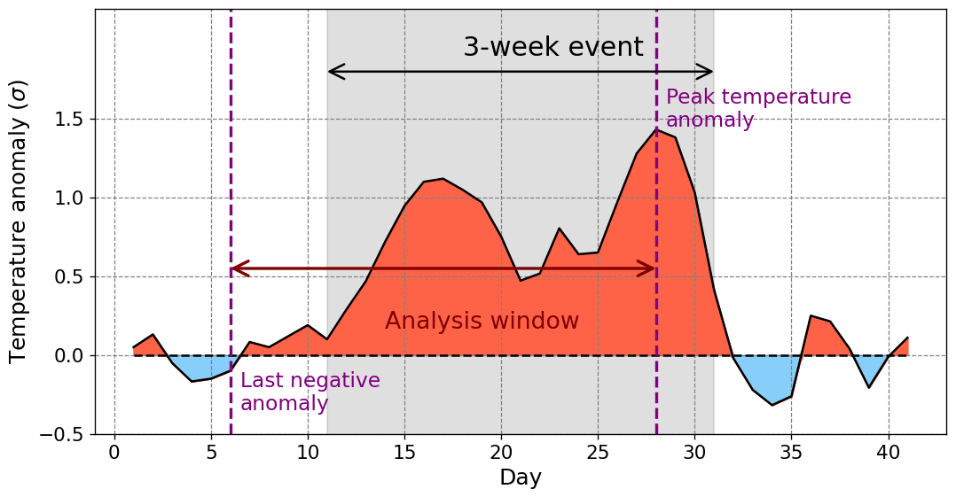
Figure 1Persistent warm and cold spell identification. From the region-averaged normalised (i.e. unitless; see Sect. 2.1) daily temperature series, a warm spell (grey shading) is identified as an extreme 3-week average anomaly (here, from days 11–31). We then identify the corresponding analysis window as the period between the last day before the event on which the temperature anomaly was negative (here day 6) and the day during the event on which the temperature anomaly peaked (here day 28). Cold spells are identified in a symmetrical way. Note that the reference day value for this example was artificially set at 0.
2.2.3 Synoptic anomalies during warm and cold spells
We then calculate anomaly maps of selected fields (Sect. 2.1) averaged over the analysis windows. Anomalies are calculated for each event within each season and each region separately. We average the different fields during the corresponding event time window and subtract the long-term average calculated over the same calendar days across the whole ERA5 record. Anomaly maps for each season and region are then averaged across events for warm and cold spells separately. We assess the statistical significance of the anomalies by calculating at each grid point their rank among a sample of 1000 anomalies obtained from randomly generated sets of events with the same distribution of duration and timing of occurrence (calendar days) as observed events. From this rank an empirical p value is obtained, which we correct for the false discovery rate (Wilks, 2016). As mentioned in the Introduction, our primary goal is not to analyse each region separately but to highlight common features between regions. To do so, we centre each anomaly map around the (geographical) median point of the corresponding region so as to be able to visually identify sets of regions with similar characteristics.
2.2.4 Temperature budget analysis
To understand the processes contributing to warm and cold spell onset and persistence, we rely on the Eulerian temperature tendency equation near the surface (on the bottommost model levels; Sect. 2.1). Assuming T is the air temperature and p the air pressure at a given grid point, the potential temperature is defined as , where , R is the gas constant for air and cp the specific heat capacity at constant pressure. The temperature tendency on sigma levels is obtained by taking the Lagrangian derivative of θ (Schielicke and Pfahl, 2022):
where the subscript |σ makes explicit that partial derivatives are taken along the sigma level. is the vertical velocity (in Pa s−1) and (u,v) the component of the horizontal (i.e. constant-sigma) wind. Equation (2) expands the temperature tendency into three common terms: the horizontal advection of temperature (at constant sigma); the adiabatic warming/cooling term linked to vertical motion; and the diabatic term, which includes contributions from sensible and latent heat fluxes. The temperature tendency, the horizontal advection and the adiabatic term can all be directly computed from the data using their analytical expressions. The diabatic term is then calculated as the residual in Eq. (2). As an additional analysis, we also consider the temperature tendency equation in the low troposphere (at 850 hPa), for which the expression is the same as in Eq. (2), however with and defined on the 850 hPa level.
We begin with the results of the quantile regression model and regionalisation approach. Deviation ratio (DR) values are overall higher in DJF than in JJA (Fig. 2), especially over oceans where the skill of the regression during JJA is very limited. This points to a weak link between the large-scale circulation and surface temperature variability over oceans during summer. This is consistent with a stable surface boundary layer, since sea-surface temperatures (SSTs) are often colder than the overlying air during summer. Selecting Z500 variability as covariate makes our approach less applicable to the tropics and subtropics because Z500 variability there is low compared to the extratropics. DR values are thus mostly low (<0.4) below 40∘ N, except in the equatorial Pacific during DJF. The high values in the Pacific are likely a result of the strong influence of ENSO-related SST variability on the tropical large-scale circulation. For the regionalisation, we only keep grid points where the DR is ≥0.4 (about 45 % of the total area in DJF and 11 %–14 % in JJA). The distributions of silhouette coefficients show a peak at (JJA cold spells), (DJF warm spells) and (JJA warm spells) (Fig. A4). The peaks are not particularly sharp, but our results do not change substantially when considering slightly different K* values. For DJF cold spells, the maximum silhouette coefficient is at K=44, but the silhouette coefficients are largely constant beyond K=23, a value we choose for K* to make the regionalisation as parsimonious as possible. Consistent with the DR maps, most regions are located in the middle to high latitudes and over continents in JJA (Fig. 3). Regions are generally highly coherent in space (also true without applying the dbscan-based filtering; not shown), except for three regions (12 in Fig. 3b, 15 in Fig. 3d and 10 in Fig. 3d). This may point either to teleconnections or to uncertainties in the regionalisation. In the tropics and subtropics, there are similarities in the regionalisation between warm and cold spells in DJF. In both cases, the algorithm detects a region along the equatorial Pacific Ocean, most likely related to ENSO and its large imprint on the tropical circulation. The region even extends to the equatorial Indian Ocean for persistent warm spells. We also find similar regions in the subtropics (3, 4, 8 and 9 in Fig. 3a and 17, 13, 8 and 11 in Fig. 3a). Regions are generally bigger in DJF than in JJA, for both cold and warm spells, especially in terms of zonal extent. They cover an average of 4.1–4.3 × 10⁶ km2 in DJF (excluding the handful of tropical regions) against 1.3–1.6 × 10⁶ km2 in JJA, with a mean zonal extent of 3000–3500 km in DJF against 1500–1700 km in JJA. These figures are naturally influenced by the choice of optimal region number but nevertheless indicate a tendency for larger spatial footprints of persistent temperature extremes in DJF compared to JJA.
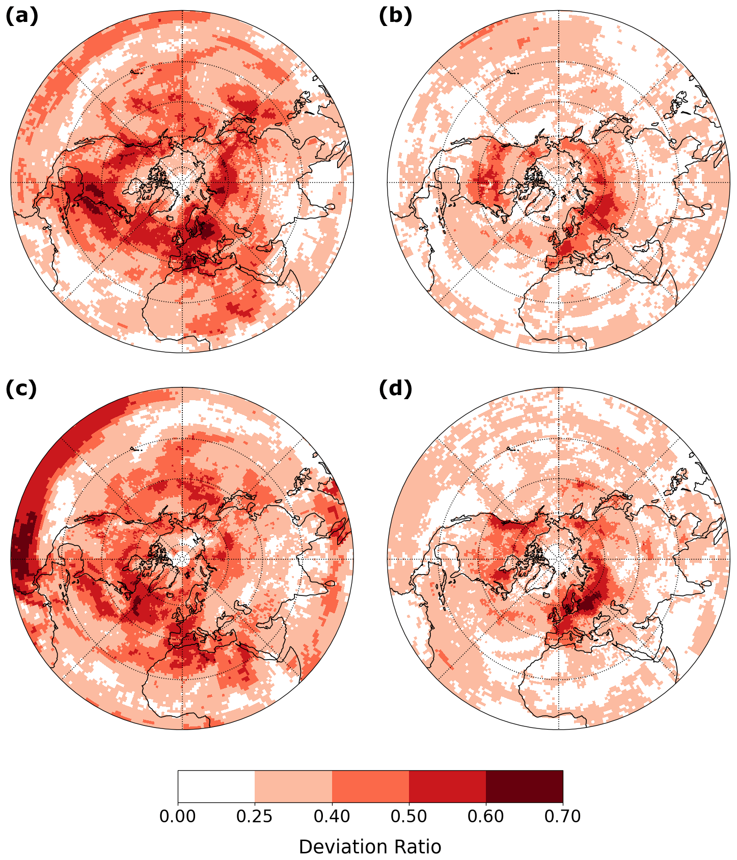
Figure 2Goodness of fit for the quantile regression model: (a) DJF cold spells, (b) JJA cold spells, (c) DJF warm spells and (d) JJA warm spells.
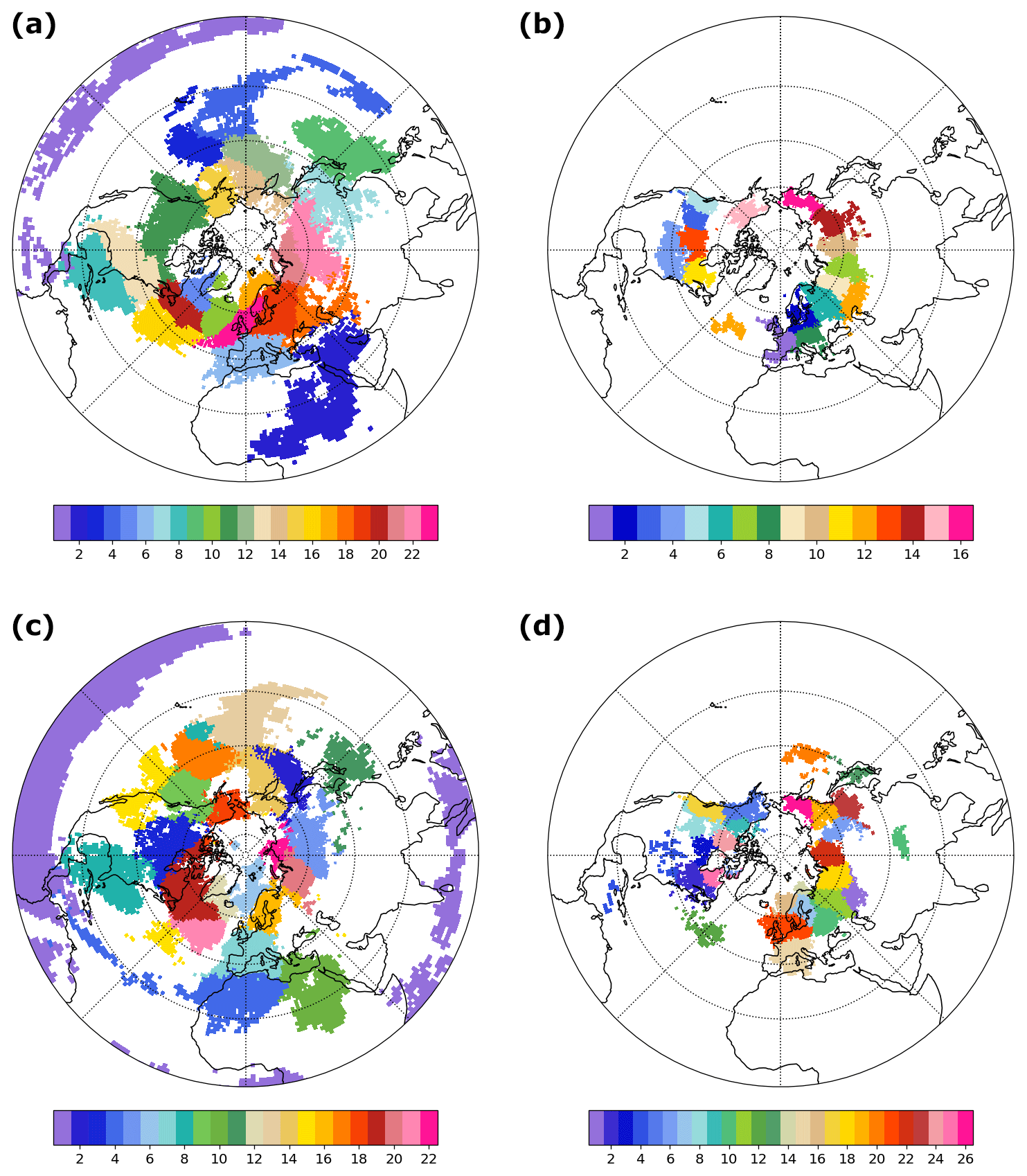
Figure 3Regionalisation results: (a) DJF cold spells, (b) JJA cold spells, (c) DJF warm spells and (d) JJA warm spells.
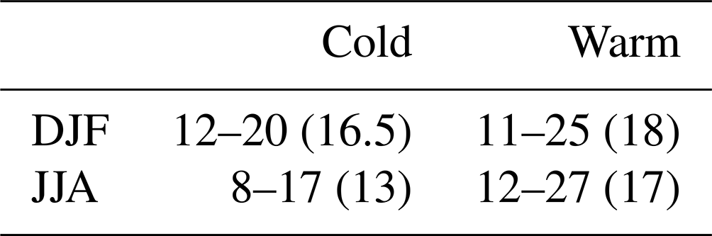
With regions now identified, we calculate the lengths of the analysis windows as described in Fig. 1 and Sect. 2 to assess the timescale(s) associated with the build-up and persistence of warm and cold spells. Results in Table 1 (see also Fig. A3) show that in all cases, persistent warm and cold spells develop over a 1–4 week period, with an average window length of 2–2.5 weeks. These numbers do not noticeably change for a 4-week window and are only slightly lower for a 2-week window (average of 1.5–2 weeks; see Tables A1 and A2). There is however a large variability in the analysis window length from one event to the other (coefficient of variation ≈ 0.5 for most regions). Note that because we calculate synoptic anomaly maps for each event separately (Sect. 2.2.3), longer events do not get more weight than shorter ones in the results. In the following, we analyse the circulation and the temperature budget anomalies during DJF and JJA warm and cold spells separately. We refrain from discussing the particulars of any one of the regions specifically, instead focusing on the robust features that can be found across all regions or sub-groups of regions.
Table 1Analysis window length (in days) for warm and cold spells: inter-region range and median (between brackets; see definition in Fig. 1). For DJF, tropical regions 1 and 4 (Fig. 3a) and 1 (Fig. 3c) are excluded.
4.1 DJF cold spells
Comparing circulation anomaly maps across regions, we visually identify three main groups of regions with similar circulation anomalies during persistent DJF cold spells (tropical and sub-tropical regions being excluded from the analysis; Fig. 4). The first group consists of 11 regions where cold spells are linked to upstream blocking, either to the west or to the northwest. For the three regions of the second group, blocking is also present but downstream to the northeast. Finally, the third group consists of five high-latitude regions where cold spells are associated with a southward migration of the polar jet.
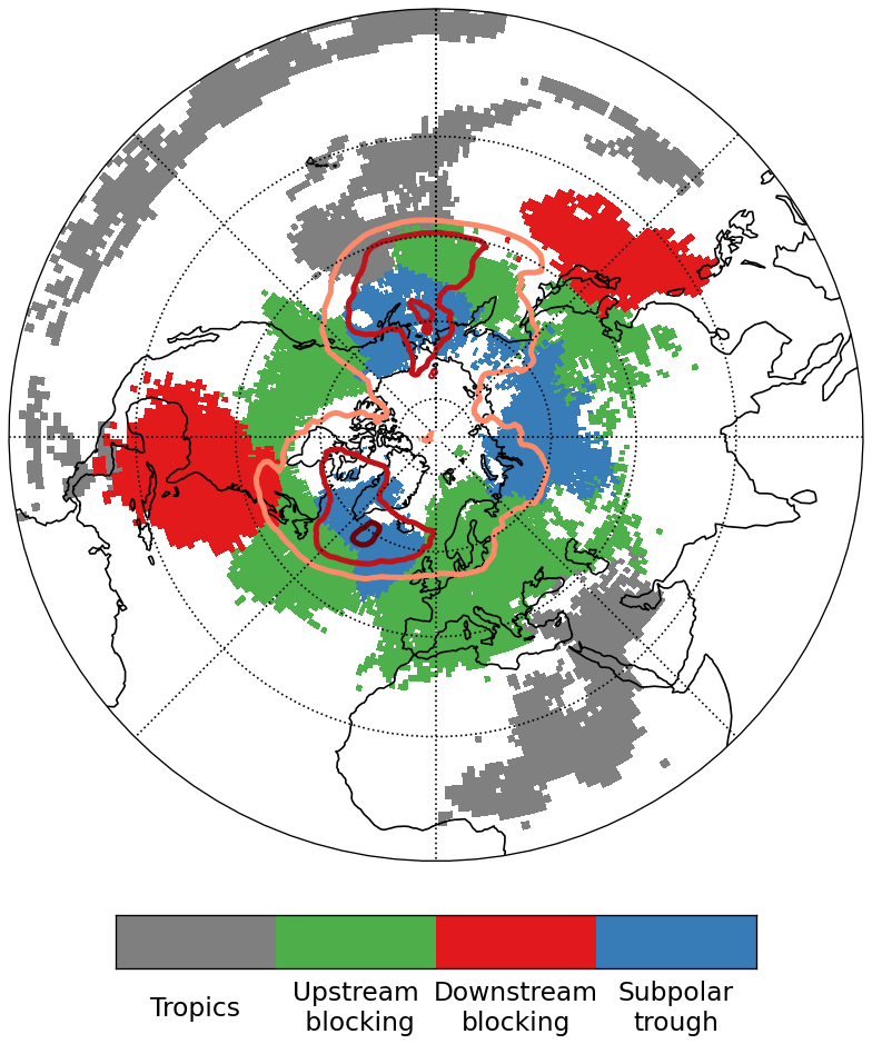
Figure 4Classification of extratropical DJF cold spell regions according to their associated concurrent main circulation anomalies: upstream blocking (green), downstream blocking (red) and subpolar lows (blue). Tropical regions (excluded from the discussion) are shown in grey. The DJF-mean blocking frequency is also indicated by the thick contours (2.5 %, 5 % and 7.5 %).
4.1.1 Upstream blocking
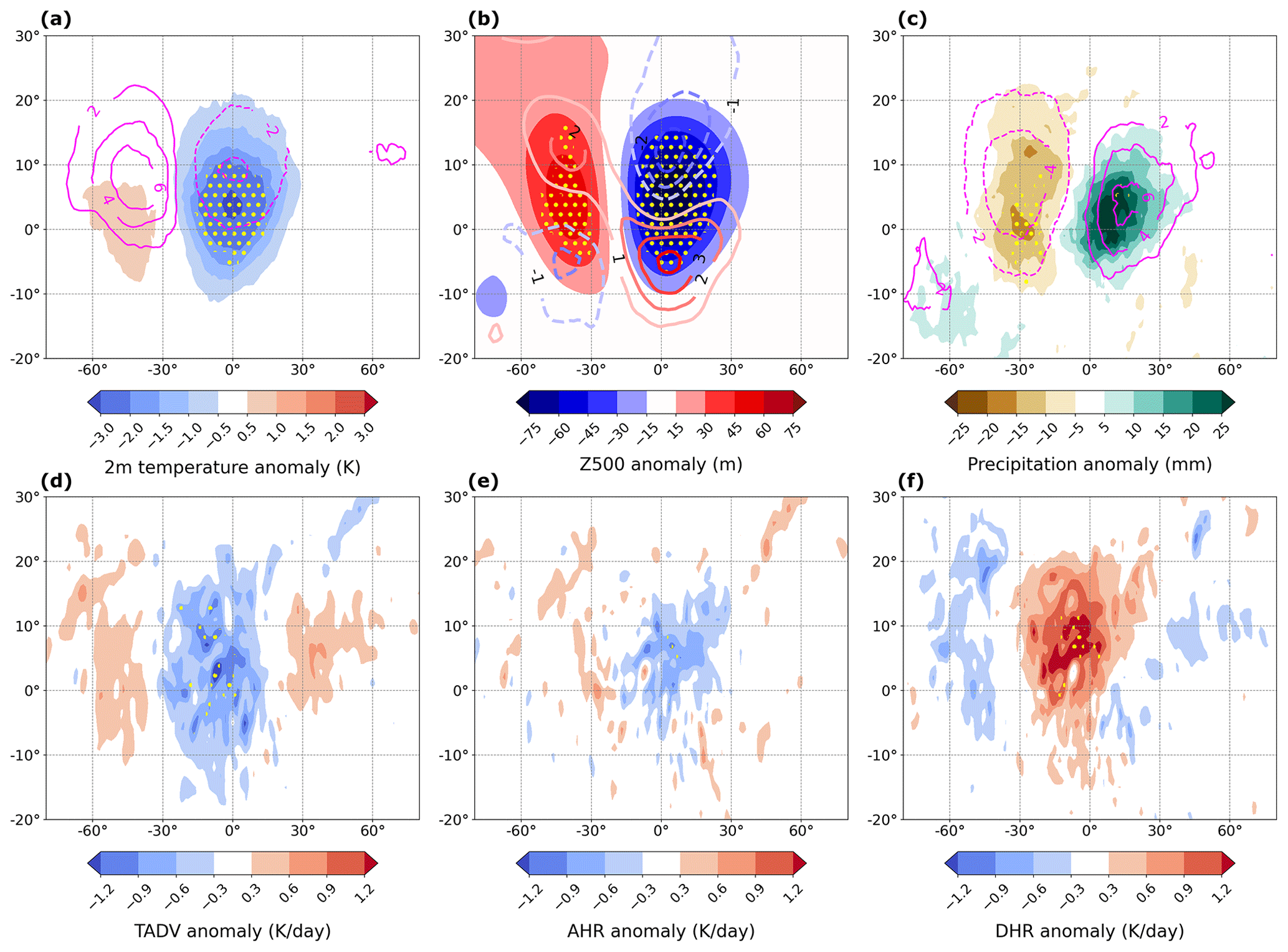
Regions where cold spells occur alongside upstream blocking are mainly located north of 40∘ N on each side of the North Atlantic and Pacific oceans (Fig. 4). Most of them are located south and southwest of the two main blocking regions (Greenland and the Bering Strait). The distribution of average blocking anomalies for this group of regions shows enhanced blocking frequency and anomalously high Z500 to the west and northwest of the area with colder-than-average temperatures, which is located under a pronounced trough (Fig. 5a, b). The mid-latitude jet is displaced equatorwards of the cold region (Fig. 5b). Consistent with the circulation anomalies, cyclone activity and precipitation are suppressed downstream of the block, over the western half of the cold region, but enhanced downstream of the trough, especially in the left exit region of the jet streak (Fig. 5c). The near-surface temperature budget anomalies show that cold anomalies arise exclusively from cold-air advection. The advection is partly compensated for by near-surface diabatic warming, likely in the form of surface sensible heat flux and enhanced radiative warming from clouds in the eastern half of the region. At 850 hPa, cold-air advection is partly compensated for by adiabatic warming from the descent in the western part of the region (Fig. A5b, c).
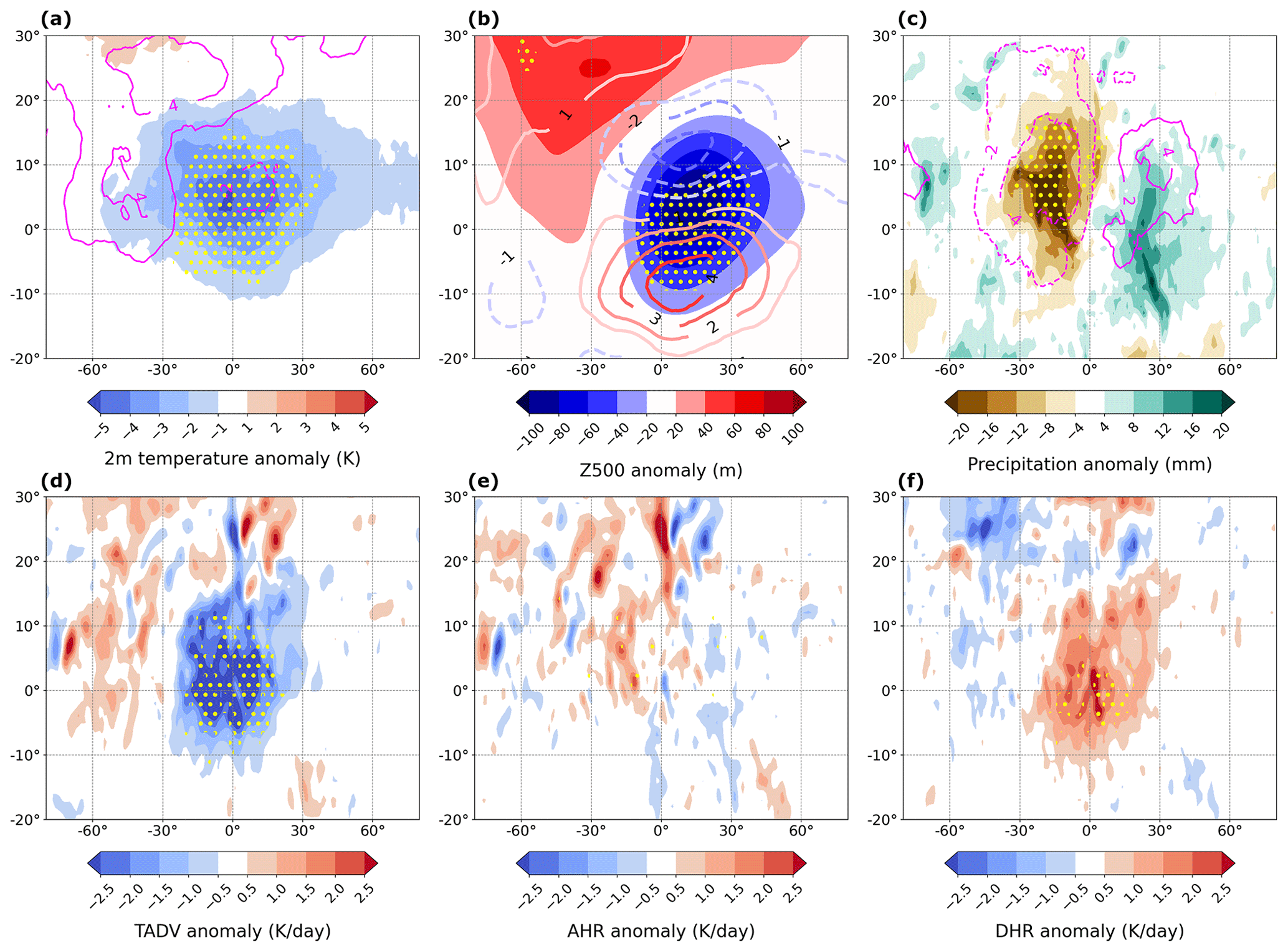
Figure 5Average anomalies for regions where DJF cold spells are linked to upstream blocking (shown in green in Fig. 4): (a) 2 m temperature (shaded contours) and blocking frequency (contour lines, in %), (b) Z500 (shaded contours) and 200 hPa wind speed (contour lines, in m s−1), (c) total precipitation (shaded contours) and cyclone frequency (contour lines, in %), (d) near-surface temperature advection, (e) near-surface adiabatic heating rate, and (f) near-surface diabatic heating rate. The yellow hatching in all panels indicates areas where anomalies of shaded fields are of the same sign and statistically significant at the 10 % level for more than two-thirds of the regions.
4.1.2 Downstream blocking
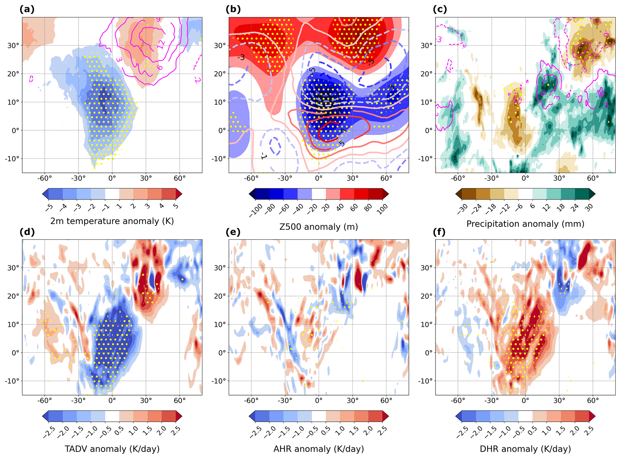
Persistent cold spells can also occur upstream of a block, as in the three regions located on the eastern margins of North America and Asia, between 20 and 40∘ N (see Figs. 3a and 4). Although the average anomalies are quite noisy due to the small number of regions, some robust features emerge. Cold anomalies occur below a zonally elongated trough that stretches to the southwest and south of a strong atmospheric block (Fig. 6a, b). A jet streak is present along the southern edge of the trough (Fig. 6b). As in the previous case, precipitation and cyclone frequency are below average in the western half of the trough and below the downstream block but higher in the eastern half of the domain (Fig. 6c). Cold surface anomalies are again caused by substantial near-surface cold advection of several kelvin per day (Fig. 6d). These large values are almost surely related to the steep zonal temperature gradient between the cold continents to the west and the relatively warm oceans to the east. The advection of cold and dry continental air masses over the ocean is then partly balanced by large positive surface heat fluxes found in the diabatic term (Fig. 6f). This picture is consistent with the precipitation anomalies. Dry conditions prevail over the western, continental half due to large-scale descent and advection of cold and dry air. Over the eastern, oceanic half, wet conditions prevail, as cold-air advection over the warm ocean surface increases surface sensible and latent heat fluxes along with the overall baroclinicity, which combines with quasi-geostrophic ascent to create an environment conducive to cyclone formation.
4.1.3 Subpolar troughs
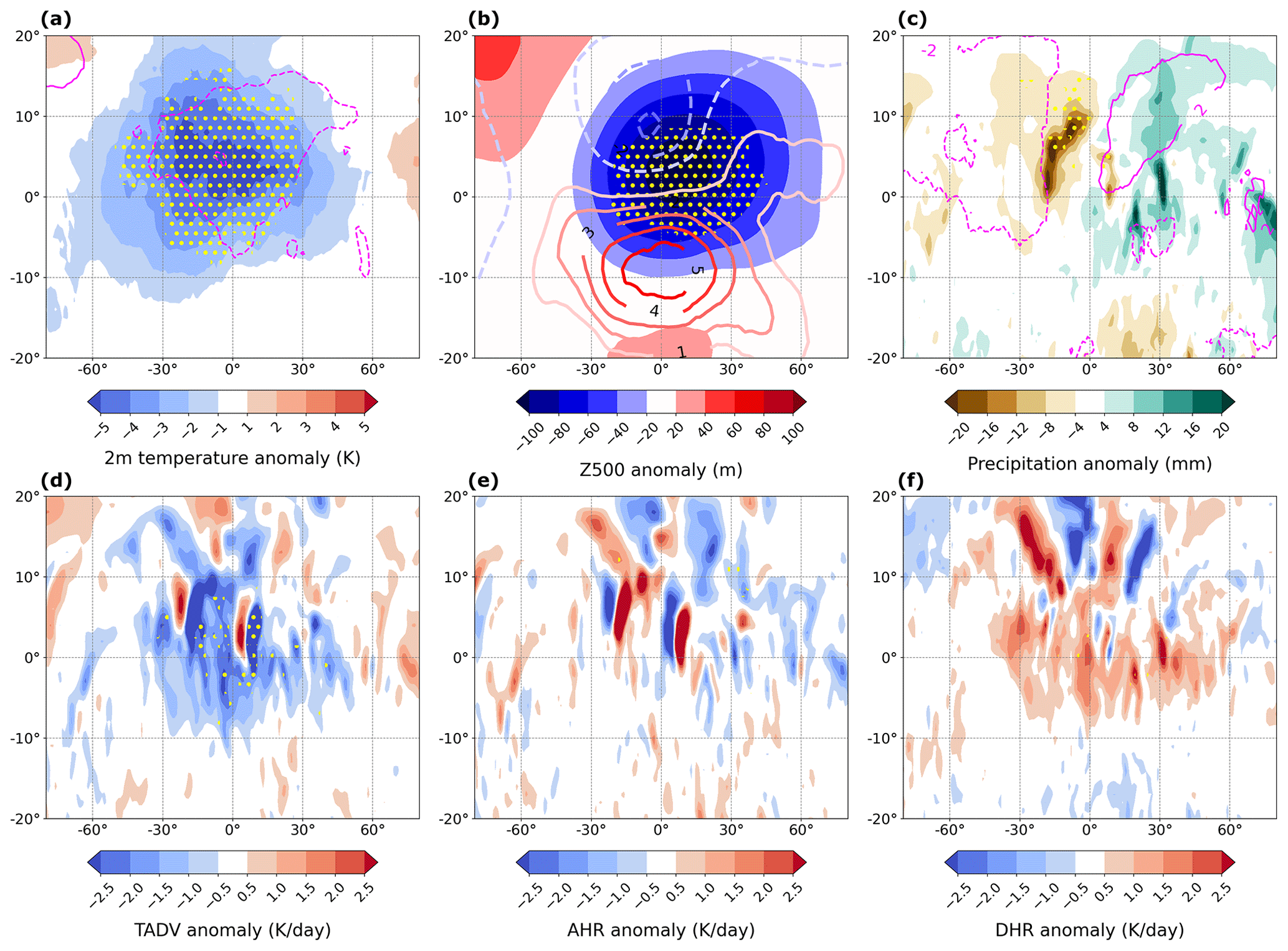
The final group of regions is restricted to the high latitudes primarily below the main blocking centres in the North Atlantic and Pacific oceans but also in northern Siberia, between 45 and 135∘ E. There, persistent cold spells occur in conjunction with suppressed blocking activity (Fig. 7a). A high is sometimes present to the west of the cold region, which is located under a deep trough, while the polar jet is shifted equatorwards (Fig. 7b). Although the regions are of a similar size to the ones from other groups, statistically significant cold anomalies extend over a much larger range of longitudes, and their magnitude tends to be larger as well (Fig. 7a). In keeping with the low specific moisture levels at high latitudes in winter, precipitation and cyclone frequency anomalies are quite small, though their pattern is similar to previous cases (Fig. 7c). The anomalies of temperature budget terms are noisy, probably because of orography, but the temperature balance remains similar to the other two region groups. Cold advection dominates the temperature tendency equation, partly balanced by diabatic warming, likely resulting from surface-to-atmosphere heat transfers and enhanced radiative warming below clouds in the east of the region. Note that the subpolar regions in Fig. 4 are far enough from the pole that cold advection from higher latitudes is possible. Farther north, advection plays a smaller role and radiative cooling drives the negative temperature tendencies (Messori et al., 2018).
4.2 JJA cold spells
Persistent cold spells in summer show very consistent circulation features across all regions, similar to the “upstream blocking” group for DJF cold spells (Figs. 5 and 8). An anomalous ridge (often flagged as a block) is present directly to the west of the cold region. The cold region is under a trough (Fig. 8b). The jet is again meridionally amplified and displaced equatorwards to the south of the cold anomalies (Fig. 8b). Precipitation and cyclone frequency anomalies are shifted westward compared to those from Fig. 5. Wet anomalies are located directly over the eastern half of the cold region, and dry anomalies are centred between the ridge and the trough, hardly overlapping with the cold region itself (Fig. 8c). Thus, while cold/dry conditions dominate in DJF, we find that in JJA cold/wet conditions are more prevalent. Temperature budget anomalies show an important difference from DJF cold spells. While temperature advection is still the main contributor to negative temperature tendencies, adiabatic cooling also plays a significant role directly below the trough (Fig. 8d, e). At 850 hPa the contribution from adiabatic cooling is even more important (though not as statistically significant) than cold advection in the eastern half of the cold region (Fig. A5d, e). Negative temperature tendencies are partly balanced by the diabatic term, in which surface heat fluxes probably dominate, although a contribution from the long-wave budget (decreased nighttime cooling below clouds) is also possible (Fig. 8f).
4.3 DJF warm spells
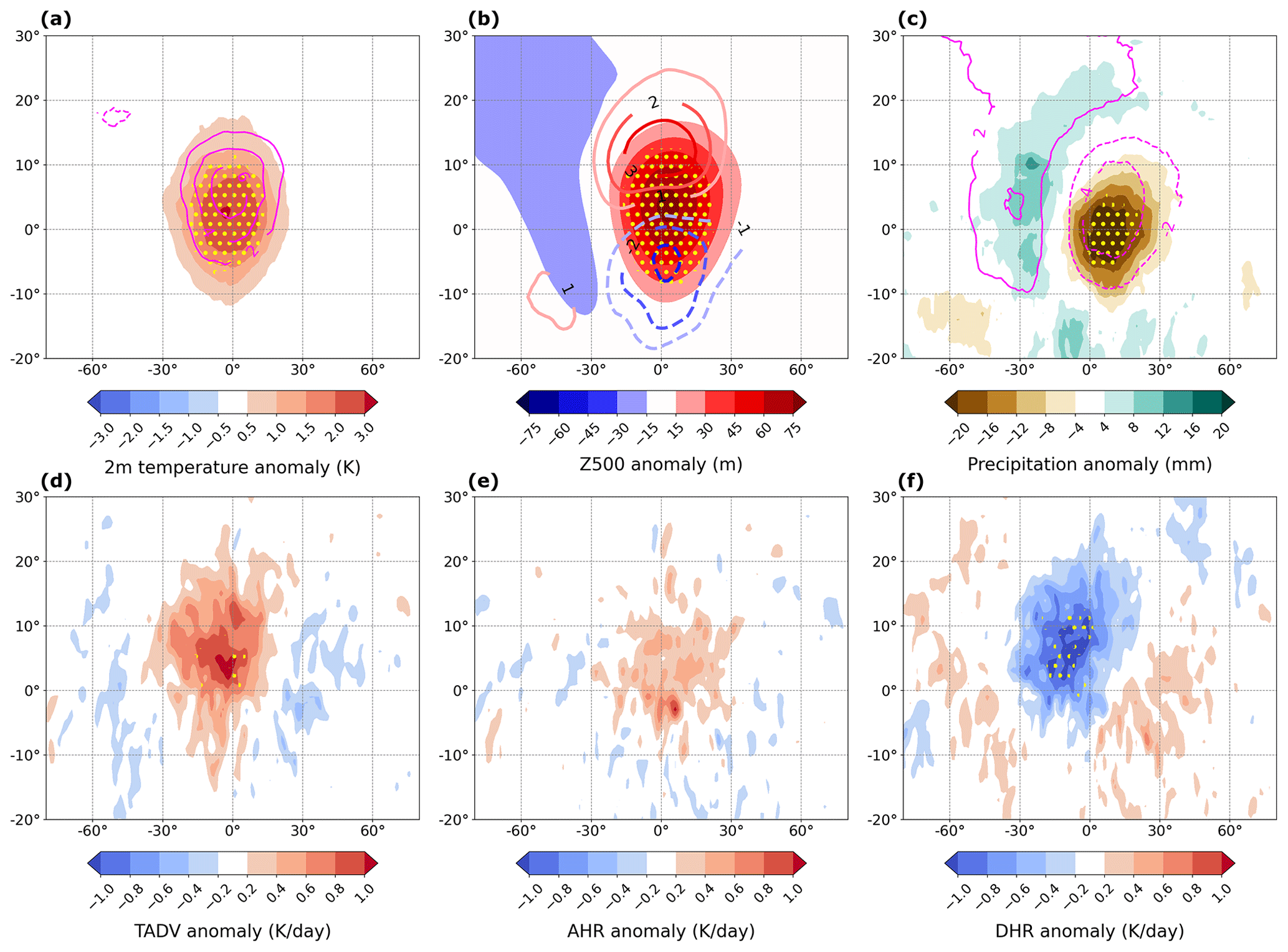
Synoptic conditions associated with persistent DJF warm spells in the extratropics are all characterised by significant positive Z500 anomalies (partly) above the warm region (Fig. 9a, b). This anomalous ridge allows for significant warm advection at the surface, which is only partly balanced by the diabatic term (Fig. 9d, f). Cyclone frequency anomalies are opposite to those found during cold spells. The western and central parts of the warm region experience wetter-than-average conditions with more frequent cyclones, while dry anomalies occur mostly in the eastern third, on the downstream side of the ridge (Fig. 9c). The exact location of the ridge relative to the warm region varies quite a lot, in keeping with the direction of the background temperature gradient. The direction of the temperature gradient is indeed not always in the meridional direction; depending e.g. on land–ocean geometry the strongest temperature gradient might also be tilted or even zonally oriented (see Fig. 10a). In most coastal regions (eastern and western Eurasia, eastern North America), the anomalous warm advection comes from the neighbouring ocean. This means that the persistent ridge is centred to the south/southeast of the warm region in western Europe/Scandinavia/coastal Siberia (regions 7, 16 and 22; Fig. 3c) but to the north/northeast in eastern Asia (regions 14 and 19) and eastern North America (regions 2 and 8). For all other regions, warm advection primarily comes from the south (Fig. 10a), and the ridge is located directly east of the warm region. In many mid- to high-latitude regions, the anomalous ridge is often flagged as a block (see hatching in Fig. 12a). This is especially true around and to the west of Greenland and the Bering Strait, where blocking is most frequent in DJF (Fig. 4). In western Europe and Scandinavia, by contrast, ocean-to-land warm advection results from the subtropical high shifting polewards, in a positive North Atlantic Oscillation-like situation (not shown). Blocking also seems relevant for regions 4 and 10 in north Africa and the eastern Mediterranean (Fig. 3c). Warm spells in these two regions indeed occur in conjunction with strong blocking over the Labrador Sea (not shown), which may possibly cause a ridge over north Africa by triggering a downstream wave train (Fig. A6).
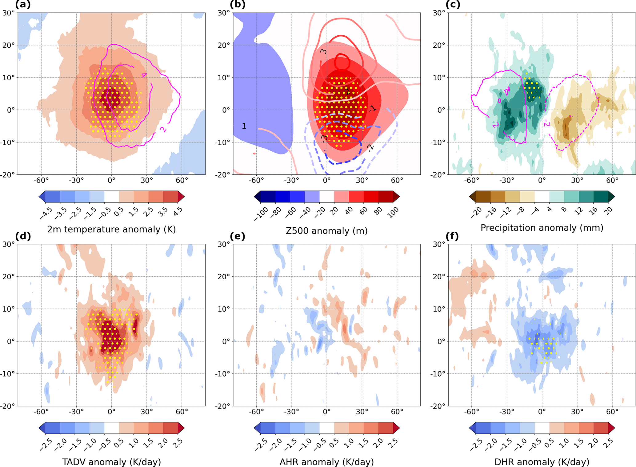
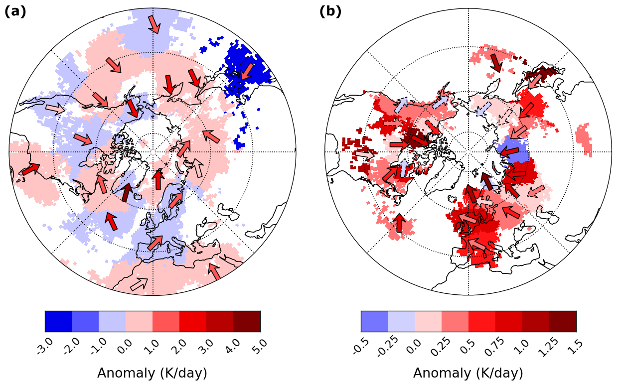
Figure 10Near-surface adiabatic warming rate (shaded) and temperature advection during persistent warm spells in (a) DJF and (b) JJA, averaged over each region. The arrows indicate the approximate direction of temperature advection and their colour the corresponding anomaly (in K d−1). The dashed arrows indicate regions where temperature advection is smaller than the adiabatic warming term.
4.4 JJA warm spells
In JJA, persistent warm spells occur for all regions directly below an anomalous ridge (Fig. 11a, b). Almost everywhere above 45∘ N, this ridge is often identified as a block (Fig. 12d). A jet streak is present polewards of the ridge (consistent with a poleward shift of the mid-latitude jet; Fig. 11b), though in a handful of cases a split jet is present (regions 7, 10, 14 and 21 over Scandinavia and regions 1, 6, 18 and 23 over Siberia; see Fig. 3d). Dry anomalies with suppressed cyclone activity prevail over most of the warm region (but mostly east and south; Fig. 11c), while precipitation is on average slightly enhanced upstream of the ridge (a signal that is not robust across regions, however). Warm anomalies at the surface come from a mix of temperature advection (essentially from lower latitudes; Fig. 10b) and adiabatic warming resulting from large-scale subsidence (Fig. 11d, e). Advection dominates, especially in the western half of the region, while adiabatic warming is at least as important in the eastern half, where large-scale descent should be the strongest. For some regions, especially at lower latitudes (40–45∘ N), adiabatic warming is even negligible. At 850 hPa, however, adiabatic warming largely exceeds advection (Fig. A7d, e). Note also that in a handful of regions, surface advection is slightly negative during warm spells, and warming results exclusively from the adiabatic term (e.g. Pacific Northwest and Alaska; Fig. 10b). The residual diabatic effects are overall robustly negative (Fig. 11f), implying that enhanced sensible heating of the lower troposphere from (short-wave) radiative warming of the ground is largely balanced by increased (long-wave) radiative cooling. The diabatic term is more negative than in winter (Fig. 9f), when ground temperatures are lower and enhanced cloud cover to the west of the regions result in long-wave warming of the surface.
4.5 Synoptic drivers of persistent warm and cold spells
Persistent summertime temperature extremes are almost always associated with a meridionally oriented circulation (wavy jet), which favours deep equatorward intrusions of cold-air or poleward intrusions of warm air (Figs. 5–9 and 11). In winter, the situation is more complex, since temperature also strongly varies with longitude due to land–sea contrasts. DJF heatwaves in coastal areas are, for instance, associated with persistent zonal flows (Fig. 10a). Advection dominates the temperature budget during cold spells in winter and summer (Figs. 5d–8d) and during warm spells in winter (Fig. 9d). Warm advection also contributes significantly to positive temperature tendencies in summer (especially at the surface and in the lowest-latitude regions; Miralles et al., 2014; Pfahl, 2014) but is sometimes exceeded by adiabatic warming (Figs. 10b and 11d, e). Our analysis of synoptic conditions and temperature budget terms during persistent warm and cold spells highlights several key ingredients for the persistence of temperature anomalies, which we now discuss in turn.
4.5.1 Atmospheric blocking
First, atmospheric blocking plays an important role in the persistence of both warm and cold spells in summer and winter. Our hemispheric perspective highlights the various influences of blocking that have previously been discussed (e.g. Carrera et al., 2004; Buehler et al., 2011; Pfahl and Wernli, 2012; Whan et al., 2016; Xie et al., 2017; Brunner et al., 2018; Jeong et al., 2021; Kautz et al., 2022). In most regions, cold spells occur most frequently downstream of persistent blocking anomalies, which drive strong cold advection through the meridional amplification of the jet. In other regions, cold spells are linked to downstream blocking through enhanced Rossby wave breaking/meridional flow amplification upstream of the block (e.g. Takaya and Nakamura, 2005). This mechanism seems relevant on the eastern side of continents, namely between 20–40∘ N in eastern North America and in eastern Asia. Both areas are upstream of the two main blocking regions in the North Atlantic and North Pacific oceans (Fig. 4). Our results also show that cold advection downstream of a block is a frequent pattern during persistent summer cold spells (Fig. 8). In summer, however, blocks have a weaker and more local effect on temperatures downstream. This is likely related to the weaker meridional temperature gradient and higher wavenumber flow in summer. Blocks also tend to occur at higher latitudes in summer (Steinfeld and Pfahl, 2019). Blocking is also critical for the persistence of winter and summer warm spells. In summer, the classic picture of a block overlying the warm surface anomalies applies to most of the identified regions, especially above 45∘ N (Fig. 12d) (Perkins, 2015; Röthlisberger and Martius, 2019). Around 35–45∘ N, however, persistent highs are more relevant than blocks for summer warm spells. Although this result may be affected by the choice of blocking identification algorithm (one based on Z500 gradients rather than PV anomalies would likely yield higher blocking frequencies in the mid-latitudes), there is good evidence that persistent subtropical ridges rather than blocks are responsible for warm spells around 35–45∘ N (Della-Marta et al., 2007; Perkins, 2015). Blocks also matter for winter warm spells (Fig. 9). Their associated circulation anomalies can result in the warm surface advection that seems essential to the onset and persistence of winter warm spells (Fig. 9d). The role of blocks in winter seems, however, mainly limited to the northwestern Atlantic and northwestern Pacific oceans (Fig. 12a). Atmospheric blocks are by definition persistent features (Schwierz et al., 2004), but their typical lifetime is usually 5–10 d, and longer blocks are extremely rare (e.g. Nabizadeh et al., 2019). The persistence of individual blocks is known to be fuelled by upstream latent heating (Steinfeld and Pfahl, 2019), but recurrent blocks are likely also key to the persistence of cold or warm spells over sub-seasonal timescales. For instance, the month-long heatwave over the Baltic in June–July 2022 (Tuel et al., 2022) and the 2010 Russian heatwave (Drouard and Woollings, 2018) were both related to several successive blocking systems.
4.5.2 Recurrent Rossby wave packets
The persistent circulation patterns during warm and cold spells can also be part of recurrent Rossby wave packets (RRWPs). In these synoptic-scale wave packets, individual troughs and ridges amplify repeatedly at the same longitudes, leading to persistent circulation anomalies frequently associated with extreme surface weather (Röthlisberger et al., 2019; Ali et al., 2022). To highlight the role of RRWPs, for each region, we look for statistically significant positive R-metric anomalies during event analysis windows in a longitude interval covering the region and up to 30∘ W of the region's westernmost points (to identify potential upstream RRWPs). Results show that persistent spells in a large number of regions are associated with significant RRWP activity (Fig. 12), most consistently across seasons and spell types over central and southern Europe. Our results for winter cold spells and JJA warm spells are highly consistent with those of Röthlisberger et al. (2019). We find strong relationships between RRWPs and persistent summer warm spells in western North America, the North Atlantic Ocean, western Europe, and northwards of the Black and Caspian seas (Fig. 12d). Interestingly, several of these regions exhibit no significant blocking anomalies during JJA warm spells. A combination of blocking directly overhead and RRWPs could therefore explain much of the circulation persistence across regions. RRWPs, however, are sometimes related to up- or downstream blocking (Röthlisberger et al., 2019). The link between RRWPs and DJF cold spells is evident in the North Pacific, the Caribbean and the Mediterranean Basin (Fig. 12a). JJA cold spells are associated with enhanced RRWP frequency in western Europe only (Fig. 12b), but we find a significant link of DJF warm spells to RRWPs in western North America, the North Atlantic and the eastern Mediterranean (Fig. 12c). In the eastern Mediterranean, these RRWPs may develop downstream of the Greenland blocking that occurs during warm spells (Berkovic and Raveh-Rubin, 2022). In western North America and the North Atlantic (region 15 in Fig. 3c, one of the few non-spatially coherent ones), RRWPs may be part of a persistent wave train associated with the so-called “North American winter temperature dipole” (Singh et al., 2016).
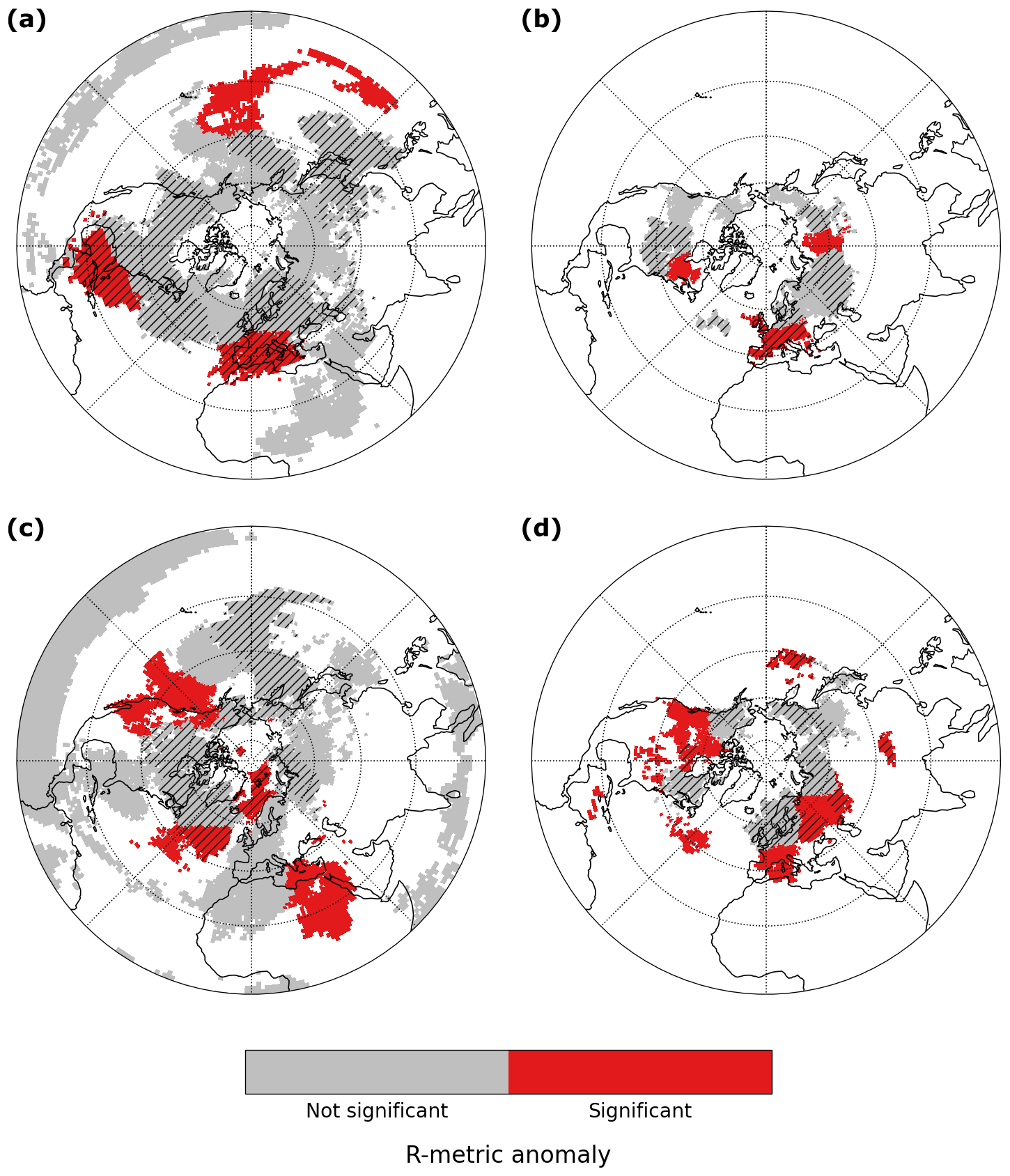
Figure 12Significance of R-metric and blocking anomalies during (a) DJF cold, (b) JJA cold, (c) DJF warm and (d) JJA warm spells. The red shading indicates regions with statistically significant positive R-metric anomalies during the corresponding events. For each region we look for R-metric anomalies above the region and up to 30∘ W of its westernmost points. Hatching indicates significant positive blocking frequencies up- or downstream of the region (a–c) or above the region (d) (not restricted to 30∘ W).
4.5.3 Land–atmosphere feedbacks
It has long been argued that land–atmosphere feedbacks can be essential for the persistence of summer warm spells (e.g. Lorenz et al., 2010; Mueller and Seneviratne, 2012; Perkins, 2015; Bartusek et al., 2021; Martius et al., 2021). Dry soils increase sensible heat fluxes to the detriment of latent heat fluxes, leading to lower-tropospheric warming and drying, which further dries the soils and stabilises the atmospheric column (Seneviratne et al., 2010; Miralles et al., 2019). This is a well-known mechanism whose role has been highlighted in several recent persistent heatwaves (e.g. García-Herrera et al., 2010; Dirmeyer et al., 2021). All our regions experience precipitation deficits during JJA warm spells, most of which are statistically significant (Figs. 11 and A8a). Over continents, these precipitation deficits translate into increased sensible heat fluxes upwards from the surface (Fig. A8b), which enhance the positive temperature anomalies and partly balance the radiative cooling seen in the negative diabatic tendencies (Fig. 11f). Regions with particularly high precipitation deficits (western North America, western Europe, Kazakhstan and eastern Siberia) also tend to exhibit the largest sensible heat flux anomalies (Fig. A8). Land–atmosphere feedbacks thus seem important for the persistence of summer warm spells, especially in transition regions where soils are neither too dry or too wet (e.g. western Europe or Scandinavia), where they have already been shown to play a role (e.g. Dirmeyer et al., 2021). It remains unclear, however, to what extent dry soils can trigger persistent heatwaves on their own or whether a dynamical forcing is required (e.g. Domeisen et al., 2023). In our case, we do not find significant precipitation deficits before the onset phase of the persistent warm spells (not shown).
4.5.4 Subpolar troughs
Finally, DJF cold spells in several high-latitude regions are linked to persistent subpolar troughs that stretch across a wide zonal band (Figs. 4 and 7). Our analysis cannot determine to what extent these troughs are part of Rossby wave trains or consist of isolated vortices, which have been documented in the Arctic where the beta effect is weak (Cavallo and Hakim, 2010). They could also occur in the framework of annular modes of variability (Arctic Oscillation). Still, Rossby wave behaviour at high latitudes supports the persistence of subpolar troughs (Woollings et al., 2023). Indeed, at high latitudes, phase and group velocities are much closer than in the mid-latitudes. Rossby wave dispersion is consequently limited. Additionally, the troughs could be part of locally triggered waves or waves triggered remotely from the tropics (by deep convection) or mid-latitudes (through baroclinicity). Among the waves initiated at lower latitudes, only the longest ones, with a slower phase speed, can reach the Arctic (Hoskins and Ambrizzi, 1993). That and the weak eddy diffusion would favour long lifetimes for subpolar cyclones. The most extreme cold spells, especially in high-latitude Eurasia, could also be related to sudden stratospheric warming events, which impact surface conditions for weeks in a row (e.g. Baldwin et al., 2021). Finally, Röthlisberger and Papritz (2023a) found that at high latitudes, slow, near-surface diabatic cooling was the dominant cause of cold extremes. We find by contrast that, in the Eulerian budget, near the surface and averaged over the multi-week timescales, diabatic cooling does not contribute significantly to persistent cold spells at high latitudes. Reasons for this discrepancy may be that our regions do not exactly capture those with strong diabatic influence in Röthlisberger and Papritz (2023a) (northeastern Siberia and North America; see Fig. 3a) and that the spatial and temporal averaging weaken the diabatic contribution (Röthlisberger and Papritz, 2023a, considered daily extremes at grid-point scale).
5.1 Model goodness of fit
As seen in Fig. 3, model goodness of fit is unequally distributed across space and time. High DR values are largely concentrated in the middle to high latitudes (polewards of 30∘ N in DJF and 40∘ N in JJA), where Z500 variability is considerably larger than in the tropics. Our selected Z500 EOFs thus primarily capture extratropical circulation variability. Our choice of Z500 as a covariate for the quantile regression is consequently not well suited for the tropics, where the streamfunction or normalised Z500 fields would yield better results. A separate model for the tropical band would also be preferable, as the tropics account for a much larger area than the extratropics, and therefore streamfunction/normalised Z500 EOFs may be biased in favour of tropical variability. Relatively small DR values above the polar circle may similarly be related to the small area these regions occupy (relative to the mid-latitudes), which weighs against them in the EOF analysis. To avoid such issues, it is conceivable to create a regionalisation based on a distance that does not rely on covariates (like the Jaccard distance or an edit-type distance; Banerjee et al., 2022). Such distances however use much less of the data than our quantile regression (only the extremes of interest) and may result in less stable and interpretable results. The regression model also performs much better in DJF than in JJA, especially over oceans. The continent–ocean contrast is particularly sharp in JJA, when DR values over oceans mostly remain below 0.4 (Fig. 3b, d). This is consistent with oceans being mostly cooler than the overlying air in summer and resulting in frequent low-level inversions, which create a more stable boundary layer than over land and make 2 m temperatures over oceans less sensitive to variations in the large-scale circulation. The large thermal inertia of the oceans similarly weakens the dependence of surface temperatures on sub-seasonal-to-seasonal variability in the large-scale circulation. Over land, surface temperatures respond much faster to forcing from the circulation. Results in Fig. 3d are in line with those of Pfahl and Wernli (2012), who found that blocking was much less relevant for summer warm spells over oceans, except over the northwestern Pacific and central North Atlantic where our model skill is also higher. Other spatial contrasts in Fig. 3 are not so easy to explain. It is notably unclear why differences in model skill between warm and cold spells exist. The ability of Z500 EOFs to capture the relevant atmospheric processes may differ regionally between warm and cold spells (due to the size, location or persistence of relevant circulation anomalies, for instance). Over land, model skill during warm spells may also be limited by the local influence of land–atmosphere feedbacks, which may not necessarily impact the large-scale circulation. Finally, topography and, in winter, snow cover also probably influence the results. We see for example that model skill is low over the Rocky Mountains in DJF. Snow cover perturbs the surface energy balance, while topography may block or steer the large-scale flow. Surface temperatures at high elevations also likely suffer from biases in ERA5.
5.2 Regionalisation
While our goal is not to discuss individual regions in detail, some general remarks can be made about the regionalisation results shown in Fig. 3. First, it is important to note that, as with any regionalisation approach, our results depend on the number of regions we select. The distance metric we use implies that regions (clusters) are areas where warm/cold spells are related to similar large-scale circulation patterns and therefore where spells tend to occur at approximately the same time. The subsequent synoptic analysis showed that our choice of regions seems consistent with the corresponding physical drivers. Too few regions would likely have blurred the significant signals in e.g. blocking location. We also find that neighbouring regions generally experience warm/cold spells at different times. In most cases, events in neighbouring regions overlap (in time) by less than 20 %. Still, our proposed regions are not necessarily the most relevant from an impacts perspective, notably because (i) the temperature thresholds we consider are relative, not absolute, and (ii) the extremeness of the temperature anomalies is softened by averaging over large scales. Second, the difference in the spatial footprint and mean zonal extent of regions between DJF and JJA, while certainly impacted by the choice of region number, is consistent with planetary waves having longer wavelengths in the cold season. This leads to larger temperature anomalies at the surface, e.g. the well-known North American dipole (Singh et al., 2016), which may correspond to regions 11 in Fig. 3a and 15 in Fig. 3c. Another important feature of the winter season is that temperature gradients are not only meridional, but also zonal. This is much less the case in summer when meridional gradients dominate. Zonal circulation can therefore lead to strong cold advection in winter. Our temperature budget analysis shows that cold spells are primarily advection driven, in both winter and summer. The cold air in summer essentially comes from the high latitudes, and a strong meridional circulation is required to bring it equatorwards, consistent with rather narrow regions in Fig. 3b. By contrast, in winter, land–ocean temperature contrasts are steep, and zonal circulations can bring about strong cold (or warm) advection, consistent with the large zonal extent of some regions like e.g. region 13 in Fig. 3a. Locally, some particularly zonally elongated regions, like regions 6 and 23 over Europe in Fig. 3a, are also likely related to strong zonal circulations (in this case the North Atlantic Oscillation) that can lead to persistent surface temperature patterns. Further differences in the regionalisation between winter and summer may be due to the seasonality of blocking (Steinfeld and Pfahl, 2019) or RRWPs (Röthlisberger et al., 2019) (in terms of location, extent and intensity). Finally, it is not straightforward to compare our regionalisation results to previous findings because (i) we take a hemispheric perspective, (ii) we look at long (3-week) cold and warm spells, and (iii) we limit ourselves to regions where the quantile regression model skill is high. Most previous studies are indeed limited to specific areas (Europe in particular) and focus on shorter-term events, chiefly heatwaves. Figure A1 shows that while there is certainly a lot of overlap between our 21 d spells and more traditional 3 d extremes, the two are not the same, notably during summer (Fig. A1b, d), which makes a direct comparison difficult. Still, over Europe during summer, our results are in general agreement with those of Carril et al. (2008), who, from EOFs of monthly temperature anomalies, found a clear tripole structure between northwestern Europe, the Euro-Mediterranean and eastern Europe/western Russia, similar to regions 10, 15 and 21 in Fig. 3d. Stefanon et al. (2012) and Pyrina and Domeisen (2023) likewise both found six spatial clusters across Europe based on the simultaneity of hot summer days, including a North Sea cluster comparable to region 21 in Fig. 3d, a western European cluster (region 15), a Scandinavian cluster (region 7), an eastern European cluster (region 10) and a Russian cluster (region 11). Some of the typical European heatwave patterns of Felsche et al. (2023) are also similar to our Fig. 3d results. Regarding cold spells, Xie et al. (2017) detected three main patterns of winter cold waves in North America (east, northwest and centre), two of which bear some resemblance to regions 11 and 13 in Fig. 3a. Region 11 is also similar to the North American region of cold outbreaks triggered by sudden stratospheric warmings identified by Kretschmer et al. (2018). The analysis of circulation anomalies during persistent warm and cold spells supports the statistical and physical relevance of our regionalisation. Identified regions are clearly different when it comes to the physical mechanisms responsible for persistent temperature anomalies. For instance, warm spells in the Euro-Mediterranean are linked to a persistent subtropical ridge, while spells in northwestern Europe are connected to blocking at higher latitudes (Fig. 10b; Carril et al., 2008; Sousa et al., 2018). Noticeable similarities between our results and those of Röthlisberger et al. (2019) on the influence of RRWPs also suggest that our regionalisation is physically meaningful. We note finally that the size of many obtained regions is comparable to that of typical atmospheric blocks (Croci-Maspoli et al., 2007; Nabizadeh et al., 2019) and associated temperature anomalies (e.g. Carrera et al., 2004; Buehler et al., 2011; Whan et al., 2016; Schaller et al., 2018; Sousa et al., 2018). Given how relevant blocking is for the persistence of extreme temperatures, this suggests that our choice of optimal region number is justified.
5.3 Other potential drivers of persistent warm and cold spells
We focus here on the regional, synoptic-scale patterns associated with persistent warm and cold spells in the extratropics. In particular, we do not discuss potential remote influences on the extratropical circulation that could modulate the likelihood and persistence of surface temperature extremes. Notable among these are SSTs and the Madden–Julian Oscillation (MJO). Both tropical and extratropical SSTs impact the extratropical circulation at sub-seasonal to seasonal timescales relevant for our study. Tropical SST anomalies (and the MJO) modulate deep convection and the resulting Rossby wave trains that propagate polewards (e.g. Lin and Brunet, 2018). Temperature extremes in the mid-latitudes are for instance known to be influenced by ENSO (e.g. Arblaster and Alexander, 2012; Li et al., 2017; Dai and Tan, 2019). The MJO also influences cold-air outbreaks in North America (Moon et al., 2012) and eastern Asia (Abdillah et al., 2018). In the extratropics, SST anomalies can also lead to storm track shifts or substantial regional circulation anomalies that impact surface weather (Hoskins and Karoly, 1981; Brayshaw et al., 2008). For example, North Atlantic SST anomalies matter for European summer heatwaves (Duchez et al., 2016; Mecking et al., 2019), and North Pacific SSTs modulate cold spells in North America (Li et al., 2017). Our regionalisation could therefore be used to identify the potential SST or tropical circulation anomalies associated with persistent warm and cold spells and relate them to the circulation anomalies around the warm/cold region. As it considerably reduces the dimension of the problem, our regionalisation also makes it possible to adopt more time-intensive methods, like causal analysis, and to include more than just classical modes of SST or tropical variability as potential covariates.
5.4 Limitations of the regional averaging
While the goal of our paper is to highlight the similarities in terms of synoptic-scale anomalies during persistent regional warm/cold spells across the Northern Hemisphere, there are some limitations relative to the averaging that must be mentioned. First, while summer regions are generally confined to land (Fig. 3b, d), in winter this is not the case (Fig. 3a, c). As a consequence, averaged anomaly maps shown in Figs. 5, 6, 7 and 9 mix together land and ocean grid points. We choose not to treat land and ocean separately, but one should remember that it may affect the results in the aforementioned figures. Since cold spells are advection driven, land–ocean contrasts probably play a limited role, but for warm spells, surface heat fluxes from the ocean surface may be significant. Second, averaging over regions of different shapes and sizes, and located at different latitudes or different points of the storm tracks, also impacts the results. There is variability in synoptic anomalies, both among different events for the same region and among different regions, even ones that we grouped together (e.g. Fig. 4). For instance, the location of a block can differ across events or regions (which may even impact the persistence of the corresponding spell). This we chose not to treat, opting instead for a simplified approach which relies on the regionalisation to reduce the problem dimension and easily highlight the similarities across different locations. The analysis of individual regions will be the subject of future work. Last, we note that ERA5 is now available back to 1940 (an 83-year dataset vs. the 42-year dataset used in this study). Considering this back extension would allow us to identify many more warm and cold spells and draw more robust conclusions.
This study introduces a regionalisation for Northern Hemisphere persistent warm and cold spells in winter and summer. The regionalisation is based on the association of persistent temperature extremes with large-scale circulation variability, which we assess with quantile regression. Between 16 and 26 coherent regions are identified for summer and winter warm and cold spells across the Northern Hemisphere. Our analysis highlights the key similarities and the diversity of processes responsible for persistent temperature extremes across regions and seasons. Cold spells systematically result from northerly cold advection. Warm spells are caused by either adiabatic warming (in summer) or warm advection (in winter). Persistent cold anomalies in winter are associated with blocking upstream (Europe, west coast continental US and eastern Asia), blocking downstream (east coasts of the continents) or polar troughs (Siberia, Alaska and Greenland). Persistent cold surface anomalies are associated with dry conditions in winter but wet in summer, and persistent warm anomalies are associated with wet conditions in winter and dry conditions in summer. We also discuss some key mechanisms responsible for the persistence of temperature extremes: blocking and recurrent Rossby wave packets are important in all seasons, while land–atmosphere feedbacks matter for summer warm spells only. Our Eulerian perspective is useful to highlight synoptic conditions during persistent warm and cold spells and thus to better understand the role of the atmospheric circulation. It would be interesting to extend our results with a Lagrangian analysis to investigate parcel origin and evolution during persistent spells.
Table A1Analysis window length (in days) for 2-week warm and cold spells: inter-region range and median.
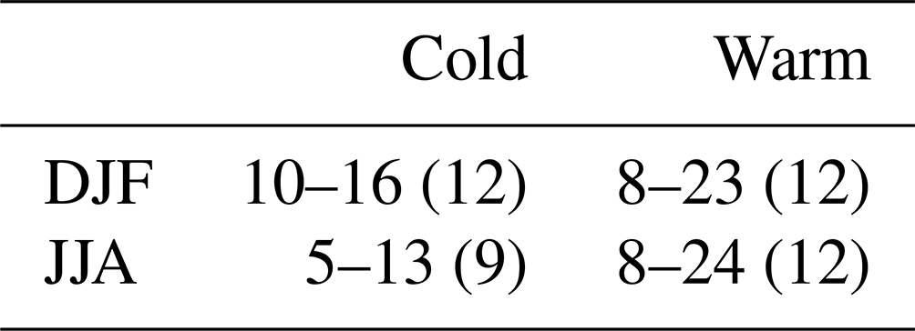
Table A2Analysis window length (in days) for 4-week warm and cold spells: inter-region range and median.

Table A3The number of identified persistent spells (roman) and the ratio of the number of 3 d events to the number of persistent spells (italics), for each season and type of spell (warm and cold). For each case, we indicate the range across clusters and in brackets the corresponding median.
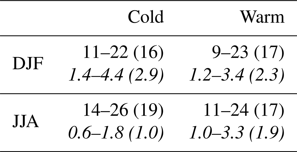
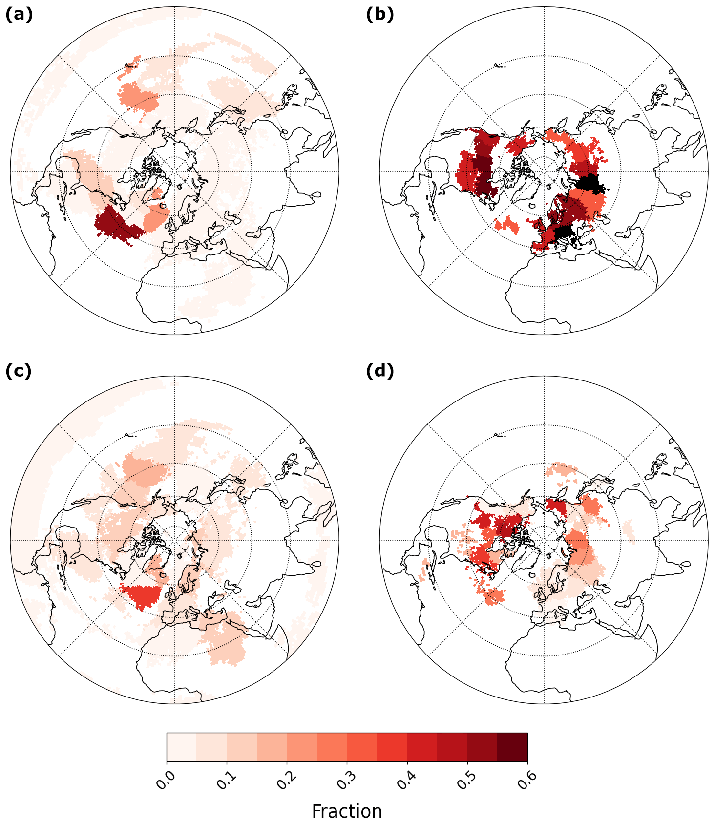
Figure A1Fraction of 21 d persistent warm/cold spells which do not include a 3 d extremely warm/cold period, for (a) DJF cold spells, (b) JJA cold spells, (c) DJF warm spells and (d) JJA warm spells. The 3 d extreme periods are defined based on continuous exceedances of the daily 5th/95th temperature percentiles in each region. In order to make sense of the values shown, we provide in Table A3 an idea of the number of persistent spells and 3 d events.
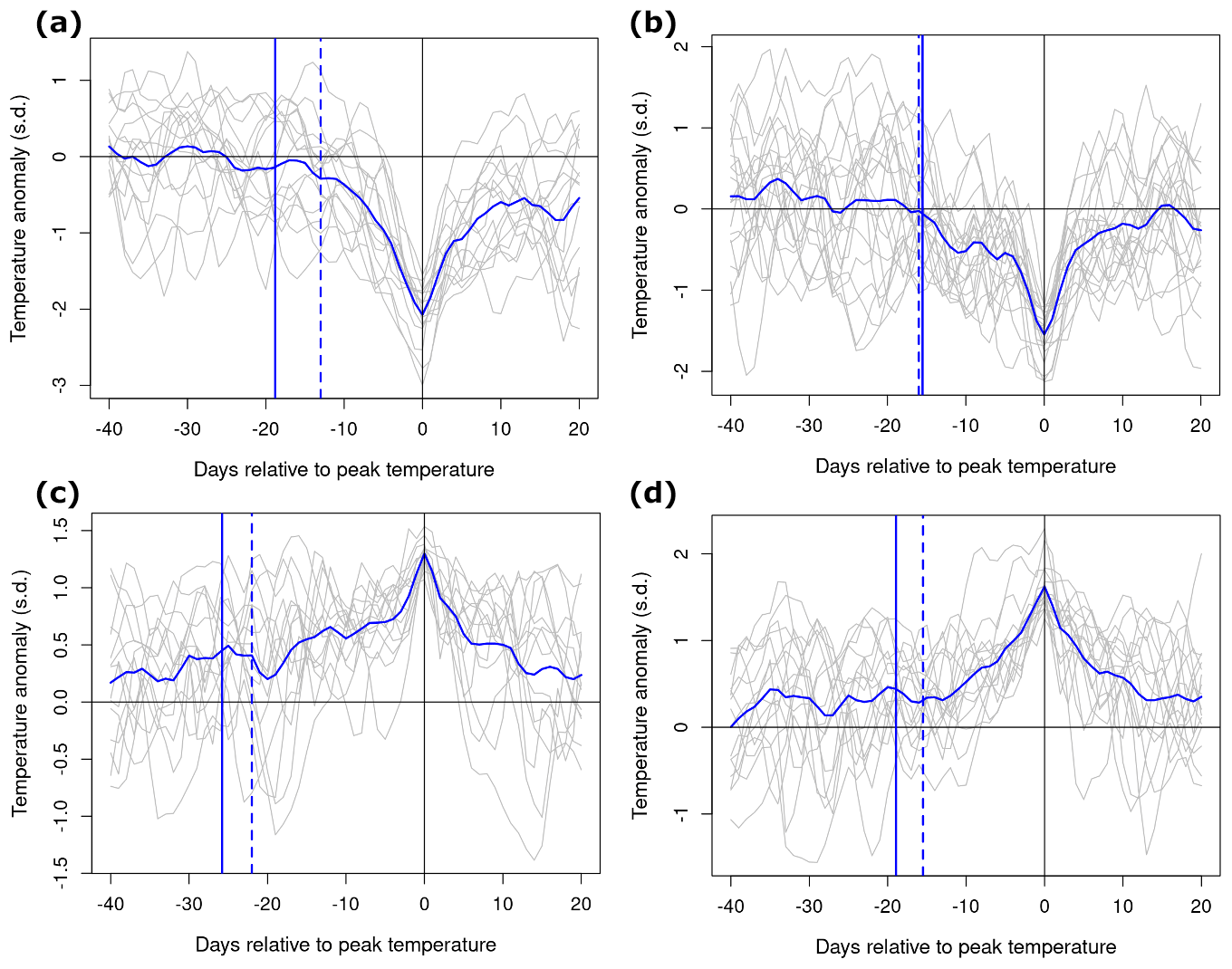
Figure A2Time series of region-average daily normalised temperature anomalies (unitless) around 3-week warm and cold spells, centred on the day of the peak temperature anomaly, for (a) DJF cold spells in region 19 (northeastern Europe), (b) JJA cold spells in region 6 (western Russia), (c) DJF warm spells in region 16 (Scandinavia) and (d) JJA warm spells in region 15 (southwestern Europe). The grey lines show the temperature evolution for individual events, and the thick blue lines show the mean. Solid (dashed) blue vertical lines indicate the mean (median) start time of the analysis windows. See Fig. 3 for the correspondence between the region numbers and their locations.
Figure A3Median window length between the last positive (negative) temperature anomaly before 3-week cold (warm) spells and the minimum (maximum) temperature anomaly in daily region-average temperature series, for (a) DJF cold spells, (b) JJA cold spells, (c) DJF warm spells and (d) JJA warm spells.
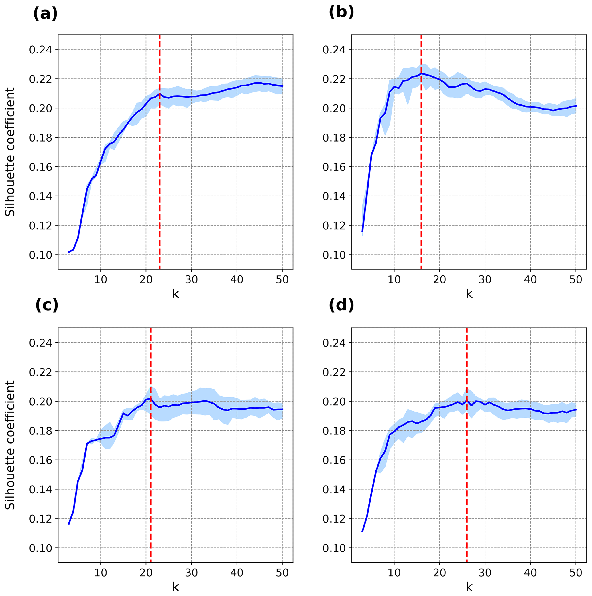
Figure A4Silhouette coefficient as a function of region number k in an ensemble of 100 PAM regionalisation results, for (a) DJF cold spells, (b) JJA cold spells, (c) DJF warm spells and (d) JJA warm spells. Shown are the ensemble mean (solid blue line) and range (blue shading) and selected number of regions (vertical red lines): (a) k=23, (b) k=16, (c) k=21 and (d) k=26.
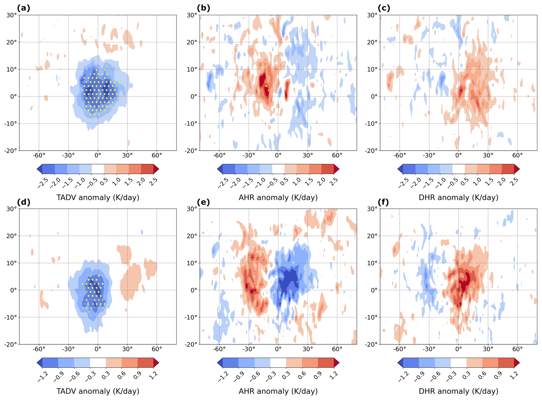
Figure A5Average temperature budget term anomalies at 850 hPa for all (a–c) DJF cold spell regions (outside the tropics; see Fig. 4) and (d–f) JJA cold spell regions: (a, d) horizontal temperature advection, (b, e) adiabatic heating rate and (c, f) diabatic heating rate. The yellow hatching in all panels indicates areas where anomalies are of the same sign and statistically significant for more than two-thirds of the regions.
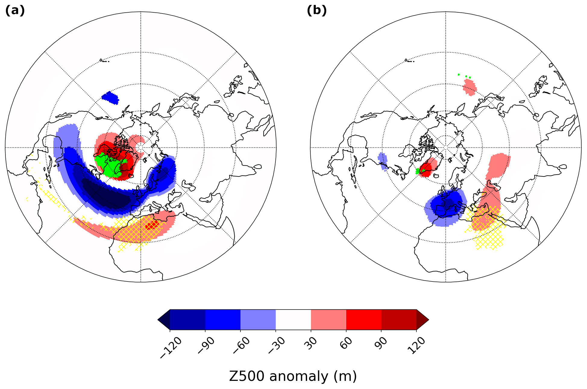
Figure A6The 500 hPa geopotential height anomalies (blue and red shading) and mean blocking frequency (green shading) during persistent DJF warm spells in regions (a) 4 and (b) 10 (yellow hatching; Fig. 3c). Only anomalies significant at the 10 % level are plotted.
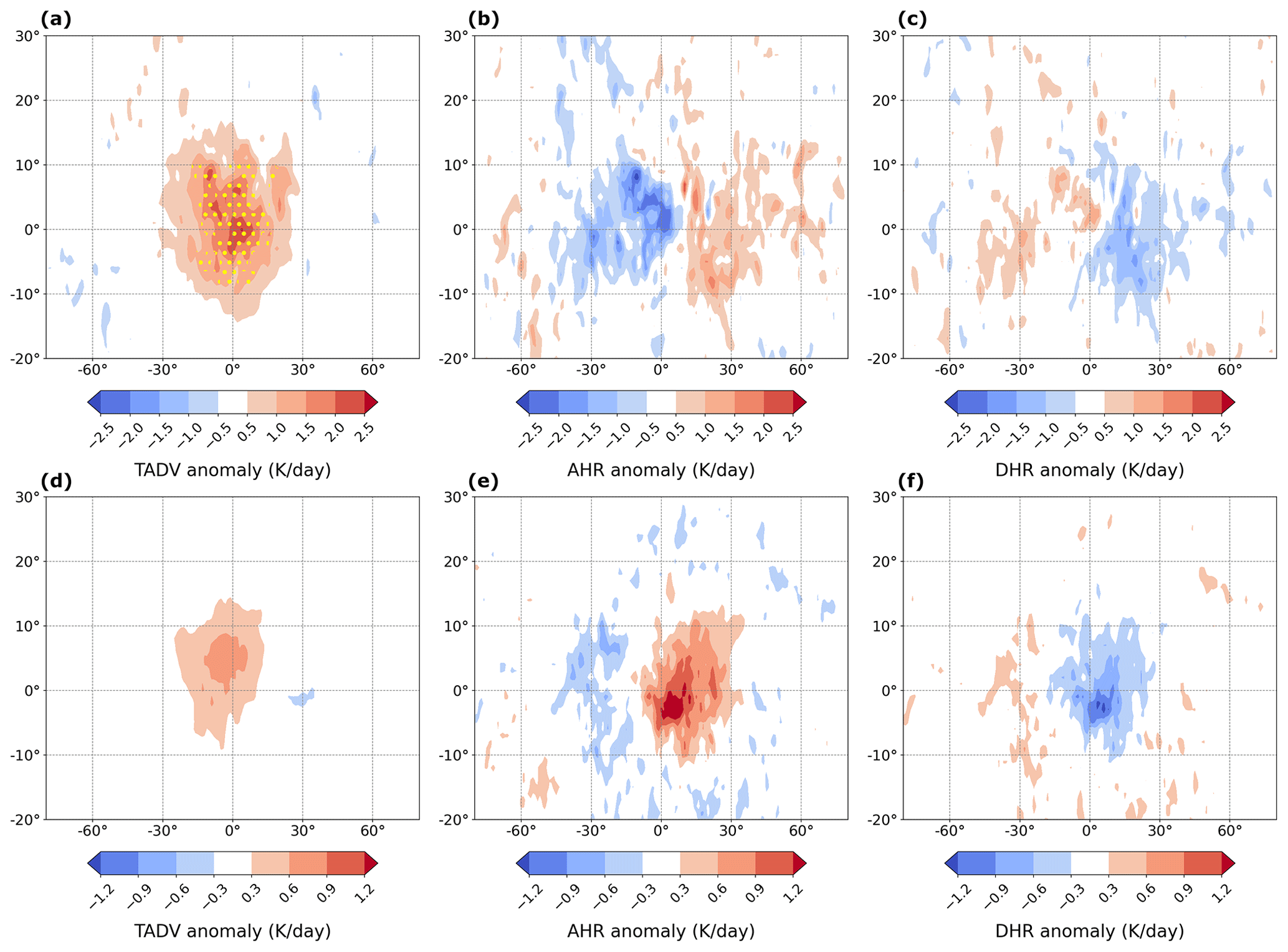
Figure A7Average temperature budget term anomalies at 850 hPa for all (a–c) DJF warm spell regions (except region 1; see Fig. 3c) and (d–f) JJA warm spell regions: (a, d) horizontal temperature advection, (b, e) adiabatic heating rate and (c, f) diabatic heating rate. The green hatching in all panels indicates areas where anomalies are of the same sign and statistically significant for more than two-thirds of the regions.
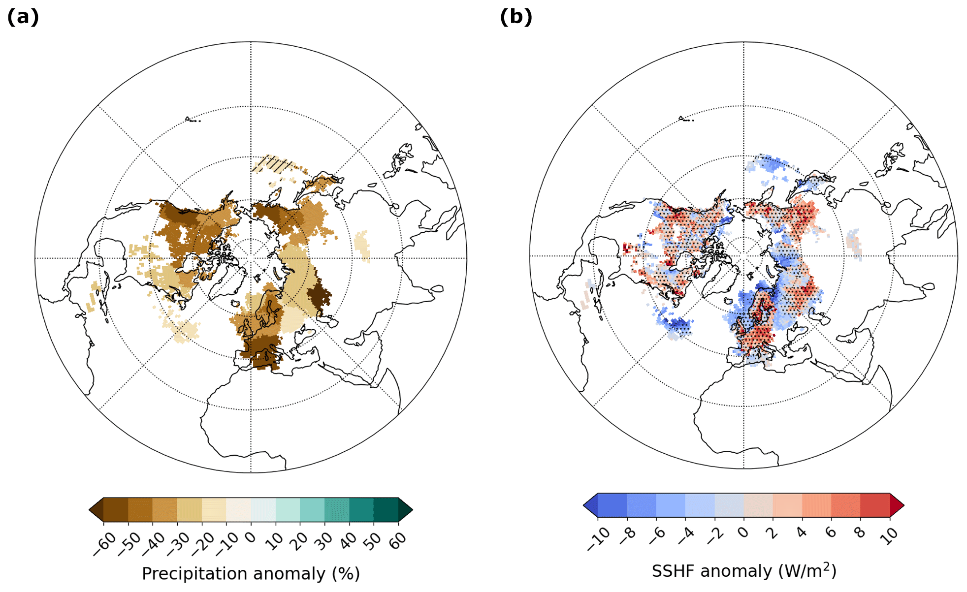
Figure A8(a) Precipitation deficits (in %) and (b) surface sensible heat flux anomalies during persistent JJA warm spells (data from ERA5). The hatching in (a) indicates the lack of statistical significance of the region-average anomaly at the 95 % confidence level. Stippling in (b) indicates statistical significance of the region-average anomaly at the 95 % confidence level. In (b), anomalies are calculated for each 1×1∘ grid cell during persistent warm spells of the corresponding region to highlight the strong land–ocean contrasts.
ERA5 reanalysis data (Hersbach et al., 2020) are available from https://doi.org/10.24381/cds.bd0915c6. The code for blocking identification is available from https://doi.org/10.5281/ZENODO.4765560 (Steinfeld, 2021), and the code to calculate the R metric is available on GitHub (https://doi.org/10.5281/zenodo.5742810; Ali, 2021). The code to reproduce our results and the regionalisation (at a 1∘ resolution) is available at https://doi.org/10.5281/ZENODO.10680180 (Tuel, 2024).
AT and OM conceived the study. AT performed all analyses and wrote the first draft with input from OM. AT and OM interpreted the results.
The contact author has declared that neither of the authors has any competing interests.
Publisher’s note: Copernicus Publications remains neutral with regard to jurisdictional claims made in the text, published maps, institutional affiliations, or any other geographical representation in this paper. While Copernicus Publications makes every effort to include appropriate place names, the final responsibility lies with the authors.
The authors gratefully acknowledge Syed Mubashshir Ali for calculating the PV data, Marco Rohrer for providing the cyclone frequency indices and Daniel Steinfeld for providing the blocking frequency indices. They also thank Heini Wernli and Matthias Röthlisberger for helpful discussions.
This research has been supported by the Schweizerischer Nationalfonds zur Förderung der Wissenschaftlichen Forschung (grant no. 178751).
This paper was edited by Pedram Hassanzadeh and reviewed by two anonymous referees.
Abdillah, M. R., Kanno, Y., and Iwasaki, T.: Tropical–Extratropical Interactions Associated with East Asian Cold Air Outbreaks. Part II: Intraseasonal Variation, J. Climate, 31, 473–490, https://doi.org/10.1175/JCLI-D-17-0147.1, 2018. a
Ali, S. M.: avatar101/R-metric, Version v1.1, Zenodo [code], https://doi.org/10.5281/zenodo.5742810, 2021. a
Ali, S. M., Röthlisberger, M., Parker, T., Kornhuber, K., and Martius, O.: Recurrent Rossby waves and south-eastern Australian heatwaves, Weather Clim. Dynam., 3, 1139–1156, https://doi.org/10.5194/wcd-3-1139-2022, 2022. a, b
Añel, J., Fernández-González, M., Labandeira, X., López-Otero, X., and de la Torre, L.: Impact of Cold Waves and Heat Waves on the Energy Production Sector, Atmosphere, 8, 209, https://doi.org/10.3390/atmos8110209, 2017. a
Arblaster, J. M. and Alexander, L. V.: The impact of the El Niño-Southern Oscillation on maximum temperature extremes, Geophys. Res. Lett., 39, L20702, https://doi.org/10.1029/2012GL053409, 2012. a
ASCE: Reliability and Resilience in the Balance – Winter Storms Report, Tech. rep., American Society of Civil Engineers, Texas Section, https://www.texasce.org/wp-content/uploads/2022/02/Reliability-Resilience-in-the-Balance-REPORT.pdf (last access: 19 February 2024), 2022. a
Baldwin, M. P., Ayarzagüena, B., Birner, T., Butchart, N., Butler, A. H., Charlton-Perez, A. J., Domeisen, D. I. V., Garfinkel, C. I., Garny, H., Gerber, E. P., Hegglin, M. I., Langematz, U., and Pedatella, N. M.: Sudden Stratospheric Warmings, Rev. Geophys., 59, e2020RG000708, https://doi.org/10.1029/2020RG000708, 2021. a
Banerjee, A., Kemter, M., Goswami, B., Merz, B., Kurths, J., and Marwan, N.: Spatial coherence patterns of extreme winter precipitation in the U.S., Theor. Appl. Climatol., 152, 385–395, https://doi.org/10.1007/s00704-023-04393-5, 2022. a
Bartusek, S., Kornhuber, K., and Ting, M.: 2021 North American Heatwave Fueled by Climate-Linked Nonlinear Interactions Between Common Drivers, in: AGU Fall Meeting Abstracts, Vol. 2021, U43D–08, https://ui.adsabs.harvard.edu/abs/2021AGUFM.U43D..08B (last access: 19 February 2024), 2021. a
Berkovic, S. and Raveh-Rubin, S.: Persistent warm and dry extremes over the eastern Mediterranean during winter: The role of North Atlantic blocking and central Mediterranean cyclones, Q. J. Roy. Meteor. Soc., 148, 2384–2409, https://doi.org/10.1002/qj.4308, 2022. a
Bernard, E., Naveau, P., Vrac, M., and Mestre, O.: Clustering of Maxima: Spatial Dependencies among Heavy Rainfall in France, J. Climate, 26, 7929–7937, https://doi.org/10.1175/JCLI-D-12-00836.1, 2013. a
Bieli, M., Pfahl, S., and Wernli, H.: A Lagrangian investigation of hot and cold temperature extremes in Europe, Q. J. Roy. Meteor. Soc., 141, 98–108, https://doi.org/10.1002/qj.2339, 2015. a, b
Biernat, K. A., Bosart, L. F., and Keyser, D.: A Climatological Analysis of the Linkages between Tropopause Polar Vortices, Cold Pools, and Cold Air Outbreaks over the Central and Eastern United States, Mon. Weather Rev., 149, 189–206, https://doi.org/10.1175/MWR-D-20-0191.1, 2021. a
Brayshaw, D. J., Hoskins, B., and Blackburn, M.: The Storm-Track Response to Idealized SST Perturbations in an Aquaplanet GCM, J. Atmos. Sci., 65, 2842–2860, https://doi.org/10.1175/2008JAS2657.1, 2008. a
Brunner, L., Schaller, N., Anstey, J., Sillmann, J., and Steiner, A. K.: Dependence of Present and Future European Temperature Extremes on the Location of Atmospheric Blocking, Geophys. Res. Lett., 45, 6311–6320, https://doi.org/10.1029/2018GL077837, 2018. a
Buehler, T., Raible, C. C., and Stocker, T. F.: The relationship of winter season North Atlantic blocking frequencies to extreme cold or dry spells in the ERA-40, Tellus A, 63, 212–222, https://doi.org/10.1111/j.1600-0870.2010.00492.x, 2011. a, b, c
Buras, A., Rammig, A., and Zang, C. S.: Quantifying impacts of the 2018 drought on European ecosystems in comparison to 2003, Biogeosciences, 17, 1655–1672, https://doi.org/10.5194/bg-17-1655-2020, 2020. a
Carrera, M. L., Higgins, R. W., and Kousky, V. E.: Downstream Weather Impacts Associated with Atmospheric Blocking over the Northeast Pacific, J. Climate, 17, 4823–4839, https://doi.org/10.1175/JCLI-3237.1, 2004. a, b
Carril, A. F., Gualdi, S., Cherchi, A., and Navarra, A.: Heatwaves in Europe: areas of homogeneous variability and links with the regional to large-scale atmospheric and SSTs anomalies, Clim. Dynam., 30, 77–98, https://doi.org/10.1007/s00382-007-0274-5, 2008. a, b, c, d, e
Cavallo, S. M. and Hakim, G. J.: Composite Structure of Tropopause Polar Cyclones, Mon. Weather Rev., 138, 3840–3857, https://doi.org/10.1175/2010MWR3371.1, 2010. a
Chapman, S. C., Murphy, E. J., Stainforth, D. A., and Watkins, N. W.: Trends in Winter Warm Spells in the Central England Temperature Record, J. Appl. Meteorol. Clim., 59, 1069–1076, https://doi.org/10.1175/JAMC-D-19-0267.1, 2020. a
China Meteorological Administration: Combined intensity of heat wave events has reached the strongest since 1961 according to BCC, http://www.cma.gov.cn/en2014/news/News/202208/t20220821_5045788.html (last access: 19 February 2024), 2022. a
Croci-Maspoli, M., Schwierz, C., and Davies, H. C.: A Multifaceted Climatology of Atmospheric Blocking and Its Recent Linear Trend, J. Climate, 20, 633–649, https://doi.org/10.1175/JCLI4029.1, 2007. a
Dai, Y. and Tan, B.: On the Role of the Eastern Pacific Teleconnection in ENSO Impacts on Wintertime Weather over East Asia and North America, J. Climate, 32, 1217–1234, https://doi.org/10.1175/JCLI-D-17-0789.1, 2019. a
Della-Marta, P. M., Luterbacher, J., von Weissenfluh, H., Xoplaki, E., Brunet, M., and Wanner, H.: Summer heat waves over western Europe 1880–2003, their relationship to large-scale forcings and predictability, Clim. Dynam., 29, 251–275, https://doi.org/10.1007/s00382-007-0233-1, 2007. a
Dirmeyer, P. A., Balsamo, G., Blyth, E. M., Morrison, R., and Cooper, H. M.: Land-Atmosphere Interactions Exacerbated the Drought and Heatwave Over Northern Europe During Summer 2018, AGU Advances, 2, e2020AV000283, https://doi.org/10.1029/2020AV000283, 2021. a, b
Domeisen, D. I. V., Eltahir, E. A. B., Fischer, E. M., Knutti, R., Perkins-Kirkpatrick, S. E., Schär, C., Seneviratne, S. I., Weisheimer, A., and Wernli, H.: Prediction and projection of heatwaves, Nat. Rev. Earth Environ., 4, 36–50, https://doi.org/10.1038/s43017-022-00371-z, 2023. a, b
Drouard, M. and Woollings, T.: Contrasting Mechanisms of Summer Blocking Over Western Eurasia, Geophys. Res. Lett., 45, 12040–12048, https://doi.org/10.1029/2018GL079894, 2018. a
Duchez, A., Frajka-Williams, E., Josey, S. A., Evans, D. G., Grist, J. P., Marsh, R., McCarthy, G. D., Sinha, B., Berry, D. I., and Hirschi, J. J.-M.: Drivers of exceptionally cold North Atlantic Ocean temperatures and their link to the 2015 European heat wave, Environ. Res. Lett., 11, 074004, https://doi.org/10.1088/1748-9326/11/7/074004, 2016. a
Ester, M., Kriegel, H. P., Sander, J., and Xiaowei, X.: A density-based algorithm for discovering clusters in large spatial databases with noise, Proceedings of the Second International Conference on Knowledge Discovery and Data Mining, August 1996, 226–231, https://www.osti.gov/biblio/421283 (last access: 19 February 2024), 1996. a
Felsche, E., Böhnisch, A., and Ludwig, R.: Inter-seasonal connection of typical European heatwave patterns to soil moisture, NPJ Clim. Atmos. Sci., 6, 1, https://doi.org/10.1038/s41612-023-00330-5, 2023. a
Galfi, V. M. and Lucarini, V.: Fingerprinting Heatwaves and Cold Spells and Assessing Their Response to Climate Change Using Large Deviation Theory, Phys. Rev. Lett., 127, 058701, https://doi.org/10.1103/PhysRevLett.127.058701, 2021. a
García-Herrera, R., Díaz, J., Trigo, R. M., Luterbacher, J., and Fischer, E. M.: A Review of the European Summer Heat Wave of 2003, Crit. Rev. Env. Sci. Tec., 40, 267–306, https://doi.org/10.1080/10643380802238137, 2010. a, b
Hartig, K., Tziperman, E., and Loughner, C. P.: Processes Contributing to North American Cold Air Outbreaks Based on Air Parcel Trajectory Analysis, J. Climate, 36, 931–943, https://doi.org/10.1175/JCLI-D-22-0204.1, 2023. a
Hersbach, H., Bell, B., Berrisford, P., Hirahara, S., Horányi, A., Muñoz-Sabater, J., Nicolas, J., Peubey, C., Radu, R., Schepers, D., Simmons, A., Soci, C., Abdalla, S., Abellan, X., Balsamo, G., Bechtold, P., Biavati, G., Bidlot, J., Bonavita, M., De Chiara, G., Dahlgren, P., Dee, D., Diamantakis, M., Dragani, R., Flemming, J., Forbes, R., Fuentes, M., Geer, A., Haimberger, L., Healy, S., Hogan, R. J., Hólm, E., Janisková, M., Keeley, S., Laloyaux, P., Lopez, P., Lupu, C., Radnoti, G., de Rosnay, P., Rozum, I., Vamborg, F., Villaume, S., and Thépaut, J.-N.: The ERA5 global reanalysis, Q. J. Roy. Meteor. Soc., 146, 1999–2049, https://doi.org/10.1002/qj.3803, 2020 (data available at: https://doi.org/10.24381/cds.bd0915c6). a
Hirschi, M., Seneviratne, S. I., Alexandrov, V., Boberg, F., Boroneant, C., Christensen, O. B., Formayer, H., Orlowsky, B., and Stepanek, P.: Observational evidence for soil-moisture impact on hot extremes in southeastern Europe, Nat. Geosci., 4, 17–21, https://doi.org/10.1038/ngeo1032, 2011. a
Hoffmann, P., Lehmann, J., Fallah, B., and Hattermann, F. F.: Atmosphere similarity patterns in boreal summer show an increase of persistent weather conditions connected to hydro-climatic risks, Sci. Rep., 11, 22893, https://doi.org/10.1038/s41598-021-01808-z, 2021. a
Hoskins, B. and Woollings, T.: Persistent Extratropical Regimes and Climate Extremes, Current Climate Change Reports, 1, 115–124, https://doi.org/10.1007/s40641-015-0020-8, 2015. a
Hoskins, B. J. and Ambrizzi, T.: Rossby Wave Propagation on a Realistic Longitudinally Varying Flow, J. Atmos. Sci., 50, 1661–1671, https://doi.org/10.1175/1520-0469(1993)050<1661:RWPOAR>2.0.CO;2, 1993. a
Hoskins, B. J. and Karoly, D. J.: The Steady Linear Response of a Spherical Atmosphere to Thermal and Orographic Forcing, J. Atmos. Sci., 38, 1179–1196, https://doi.org/10.1175/1520-0469(1981)038<1179:TSLROA>2.0.CO;2, 1981. a
Huang, J., Hitchcock, P., Maycock, A. C., McKenna, C. M., and Tian, W.: Northern hemisphere cold air outbreaks are more likely to be severe during weak polar vortex conditions, Commun. Earth Environ., 2, 147, https://doi.org/10.1038/s43247-021-00215-6, 2021. a
InfoClimat: Indicateur national français des températures, https://www.infoclimat.fr/climato/indicateur_national.php (last access: 19 February 2024), 2022. a
Jendritzky, G.: WMO/UNESCO sub-forum on science and technology in support of natural disaster reduction, chap. Impacts of extreme and persistent temperatures – cold waves and heat waves, World Meteorological Organization, Geneva, 43–52, https://whycos.org/files/hwrp/wwd2004/docs/wmo914.pdf (last access: 19 February 2024), 1999. a
Jeong, D. I., Yu, B., and Cannon, A. J.: Links between atmospheric blocking and North American winter cold spells in two generations of Canadian Earth System Model large ensembles, Clim. Dynam., 57, 2217–2231, https://doi.org/10.1007/s00382-021-05801-0, 2021. a, b
Jiménez-Esteve, B. and Domeisen, D. I.: The role of atmospheric dynamics and large-scale topography in driving heatwaves, Q. J. Roy. Meteor. Soc., 148, 2344–2367, https://doi.org/10.1002/qj.4306, 2022. a, b, c
Kautz, L.-A., Martius, O., Pfahl, S., Pinto, J. G., Ramos, A. M., Sousa, P. M., and Woollings, T.: Atmospheric blocking and weather extremes over the Euro-Atlantic sector – a review, Weather Clim. Dynam., 3, 305–336, https://doi.org/10.5194/wcd-3-305-2022, 2022. a, b
Koenker, R.: quantreg: Quantile Regression, CRAN [code], https://CRAN.R-project.org/package=quantreg, 2022. a
Kolstad, E. W., Breiteig, T., and Scaife, A. A.: The association between stratospheric weak polar vortex events and cold air outbreaks in the Northern Hemisphere, Q. J. Roy. Meteor. Soc., 136, 886–893, https://doi.org/10.1002/qj.620, 2010. a
Kretschmer, M., Cohen, J., Matthias, V., Runge, J., and Coumou, D.: The different stratospheric influence on cold-extremes in Eurasia and North America, NPJ Clim. Atmos. Sci., 1, 44, https://doi.org/10.1038/s41612-018-0054-4, 2018. a
Li, Z., Manson, A. H., Li, Y., and Meek, C.: Circulation characteristics of persistent cold spells in central–eastern North America, J. Meteorol. Res., 31, 250–260, https://doi.org/10.1007/s13351-017-6146-y, 2017. a, b, c
Lin, H. and Brunet, G.: Extratropical Response to the MJO: Nonlinearity and Sensitivity to the Initial State, J. Atmos. Sci., 75, 219–234, https://doi.org/10.1175/JAS-D-17-0189.1, 2018. a
Lorenz, R., Jaeger, E. B., and Seneviratne, S. I.: Persistence of heat waves and its link to soil moisture memory, Geophys. Res. Lett., 37, L09703, https://doi.org/10.1029/2010GL042764, 2010. a
Lowe, R., Ballester, J., Creswick, J., Robine, J.-M., Herrmann, F. R., and Rodó, X.: Evaluating the Performance of a Climate-Driven Mortality Model during Heat Waves and Cold Spells in Europe, Int. J. Env. Res. Pub. He., 12, 1279–1294, https://doi.org/10.3390/ijerph120201279, 2015. a
Lyon, B., Barnston, A. G., Coffel, E., and Horton, R. M.: Projected increase in the spatial extent of contiguous US summer heat waves and associated attributes, Environ. Res. Lett., 14, 114029, https://doi.org/10.1088/1748-9326/ab4b41, 2019. a
Martius, O., Wehrli, K., and Rohrer, M.: Local and Remote Atmospheric Responses to Soil Moisture Anomalies in Australia, J. Climate, 34, 9115–9131, https://doi.org/10.1175/JCLI-D-21-0130.1, 2021. a
McKinnon, K. A. and Simpson, I. R.: How Unexpected Was the 2021 Pacific Northwest Heatwave?, Geophys. Res. Lett., 49, e2022GL100380, https://doi.org/10.1029/2022GL100380, 2022. a
Mecking, J., Drijfhout, S., Hirschi, J.-M., and Blaker, A.: Ocean and atmosphere influence on the 2015 European heatwave, Environ. Res. Lett., 14, 114035, https://doi.org/10.1088/1748-9326/ab4d33, 2019. a
Messori, G., Woods, C., and Caballero, R.: On the Drivers of Wintertime Temperature Extremes in the High Arctic, J. Climate, 31, 1597–1618, https://doi.org/10.1175/JCLI-D-17-0386.1, 2018. a
Miralles, D. G., Teuling, A. J., van Heerwaarden, C. C., and Vilà-Guerau de Arellano, J.: Mega-heatwave temperatures due to combined soil desiccation and atmospheric heat accumulation, Nat. Geosci., 7, 345–349, https://doi.org/10.1038/ngeo2141, 2014. a
Miralles, D. G., Gentine, P., Seneviratne, S. I., and Teuling, A. J.: Land–atmospheric feedbacks during droughts and heatwaves: state of the science and current challenges, Ann. NY Acad. Sci., 1436, 19–35, https://doi.org/10.1111/nyas.13912, 2019. a, b
Moon, J.-Y., Wang, B., and Ha, K.-J.: MJO Modulation on 2009/10 Winter Snowstorms in the United States, J. Climate, 25, 978–991, https://doi.org/10.1175/JCLI-D-11-00033.1, 2012. a
Mueller, B. and Seneviratne, S. I.: Hot days induced by precipitation deficits at the global scale, P. Natl. Acad. Sci. USA, 109, 12398–12403, https://doi.org/10.1073/pnas.1204330109, 2012. a
Nabizadeh, E., Hassanzadeh, P., Yang, D., and Barnes, E. A.: Size of the Atmospheric Blocking Events: Scaling Law and Response to Climate Change, Geophys. Res. Lett., 46, 13488–13499, https://doi.org/10.1029/2019GL084863, 2019. a, b
New York Times: Phoenix’s Month in Hell: A 31-Day Streak of Record Heat Ends, https://www.nytimes.com/2023/07/31/us/phoenix-heat-july.html (last access: 19 February 2024), 2023. a
NPR: Texas officials put the final death toll from last year's winter storm at 246, https://www.npr.org/2022/01/03/1069974416/texas-winter-storm-final-death-toll (last access: 19 February 2024), 2022. a
Perkins, S. E.: A review on the scientific understanding of heatwaves – Their measurement, driving mechanisms, and changes at the global scale, Atmos. Res., 164–165, 242–267, https://doi.org/10.1016/j.atmosres.2015.05.014, 2015. a, b, c, d
Perkins, S. E. and Alexander, L. V.: On the Measurement of Heat Waves, J. Climate, 26, 4500–4517, https://doi.org/10.1175/JCLI-D-12-00383.1, 2013. a
Pfahl, S.: Characterising the relationship between weather extremes in Europe and synoptic circulation features, Nat. Hazards Earth Syst. Sci., 14, 1461–1475, https://doi.org/10.5194/nhess-14-1461-2014, 2014. a
Pfahl, S. and Wernli, H.: Quantifying the relevance of atmospheric blocking for co-located temperature extremes in the Northern Hemisphere on (sub-)daily time scales, Geophys. Res. Lett., 39, L12807, https://doi.org/10.1029/2012GL052261, 2012. a, b, c
Pfleiderer, P., Schleussner, C.-F., Kornhuber, K., and Coumou, D.: Summer weather becomes more persistent in a 2 ∘C world, Nat. Clim. Change, 9, 666–671, https://doi.org/10.1038/s41558-019-0555-0, 2019. a, b
Plavcová, E. and Kyselý, J.: Temporal Characteristics of Heat Waves and Cold Spells and Their Links to Atmospheric Circulation in EURO-CORDEX RCMs, Adv. Meteorol., 2019, 2178321, https://doi.org/10.1155/2019/2178321, 2019. a, b, c
Polt, K. D., Ward, P. J., de Ruiter, M., Bogdanovich, E., Reichstein, M., Frank, D., and Orth, R.: Quantifying impact-relevant heatwave durations, Environ. Res. Lett., 18, 104005, https://doi.org/10.1088/1748-9326/acf05e, 2023. a
Pyrina, M. and Domeisen, D. I. V.: Subseasonal predictability of onset, duration, and intensity of European heat extremes, Q. J. Roy. Meteor. Soc., 149, 84–101, https://doi.org/10.1002/qj.4394, 2023. a
Reuters: Canadian wildfires could persist for rest of “marathon” summer, https://www.reuters.com/world/americas/record-setting-canadian-wildfires-could-persist-rest-marathon-summer-2023-08-11/ (last access: 19 February 2024), 2023. a
Rohrer, M., Martius, O., Raible, C. C., and Brönnimann, S.: Sensitivity of Blocks and Cyclones in ERA5 to Spatial Resolution and Definition, Geophys. Res. Lett., 47, e2019GL085582, https://doi.org/10.1029/2019GL085582, 2020. a
Rousi, E., Kornhuber, K., Beobide-Arsuaga, G., Luo, F., and Coumou, D.: Accelerated western European heatwave trends linked to more-persistent double jets over Eurasia, Nat. Commun., 13, 3851, https://doi.org/10.1038/s41467-022-31432-y, 2022. a
Rousseeuw, P. J.: Silhouettes: A graphical aid to the interpretation and validation of cluster analysis, J. Comput. Appl. Math., 20, 53–65, https://doi.org/10.1016/0377-0427(87)90125-7, 1987. a
Röthlisberger, M. and Martius, O.: Quantifying the Local Effect of Northern Hemisphere Atmospheric Blocks on the Persistence of Summer Hot and Dry Spells, Geophys. Res. Lett., 46, 10101–10111, https://doi.org/10.1029/2019GL083745, 2019. a, b
Röthlisberger, M. and Papritz, L.: A Global Quantification of the Physical Processes Leading to Near-Surface Cold Extremes, Geophys. Res. Lett., 50, e2022GL101670, https://doi.org/10.1029/2022GL101670, 2023a. a, b, c, d
Röthlisberger, M. and Papritz, L.: Quantifying the physical processes leading to atmospheric hot extremes at a global scale, Nat. Geosci., 16, 210–216, https://doi.org/10.1038/s41561-023-01126-1, 2023b. a
Röthlisberger, M., Frossard, L., Bosart, L. F., Keyser, D., and Martius, O.: Recurrent Synoptic-Scale Rossby Wave Patterns and Their Effect on the Persistence of Cold and Hot Spells, J. Climate, 32, 3207–3226, https://doi.org/10.1175/JCLI-D-18-0664.1, 2019. a, b, c, d, e, f, g
Saunders, K., Stephenson, A., and Karoly, D.: A regionalisation approach for rainfall based on extremal dependence, Extremes, 24, 215–240, https://doi.org/10.1007/s10687-020-00395-y, 2021. a
Schaller, N., Sillmann, J., Anstey, J., Fischer, E. M., Grams, C. M., and Russo, S.: Influence of blocking on Northern European and Western Russian heatwaves in large climate model ensembles, Environ. Res. Lett., 13, 054015, https://doi.org/10.1088/1748-9326/aaba55, 2018. a, b, c
Schielicke, L. and Pfahl, S.: European heatwaves in present and future climate simulations: a Lagrangian analysis, Weather Clim. Dynam., 3, 1439–1459, https://doi.org/10.5194/wcd-3-1439-2022, 2022. a
Schwierz, C., Croci-Maspoli, M., and Davies, H. C.: Perspicacious indicators of atmospheric blocking, Geophys. Res. Lett., 31, L06125, https://doi.org/10.1029/2003GL019341, 2004. a, b
Seneviratne, S. I., Corti, T., Davin, E. L., Hirschi, M., Jaeger, E. B., Lehner, I., Orlowsky, B., and Teuling, A. J.: Investigating soil moisture–climate interactions in a changing climate: A review, Earth-Sci. Rev., 99, 125–161, https://doi.org/10.1016/j.earscirev.2010.02.004, 2010. a
Singh, D., Swain, D. L., Mankin, J. S., Horton, D. E., Thomas, L. N., Rajaratnam, B., and Diffenbaugh, N. S.: Recent amplification of the North American winter temperature dipole, J. Geophys. Res.-Atmos., 121, 9911–9928, https://doi.org/10.1002/2016JD025116, 2016. a, b
Sousa, P. M., Trigo, R. M., Barriopedro, D., Soares, P. M. M., and Santos, J. A.: European temperature responses to blocking and ridge regional patterns, Clim. Dynam., 50, 457–477, https://doi.org/10.1007/s00382-017-3620-2, 2018. a, b, c
Stefanon, M., D'Andrea, F., and Drobinski, P.: Heatwave classification over Europe and the Mediterranean region, Environ. Res. Lett., 7, 014023, https://doi.org/10.1088/1748-9326/7/1/014023, 2012. a, b
Steinfeld, D.: ConTrack – Contour Tracking of circulation anomalies in weather and climate data, Zenodo [code], https://doi.org/10.5281/ZENODO.4765560, 2021. a, b
Steinfeld, D. and Pfahl, S.: The role of latent heating in atmospheric blocking dynamics: a global climatology, Clim. Dynam., 53, 6159–6180, https://doi.org/10.1007/s00382-019-04919-6, 2019. a, b, c
Takaya, K. and Nakamura, H.: Mechanisms of Intraseasonal Amplification of the Cold Siberian High, J. Atmos. Sci., 62, 4423–4440, https://doi.org/10.1175/JAS3629.1, 2005. a
Tuel, A. and Martius, O.: Subseasonal Temporal Clustering of Extreme Precipitation in the Northern Hemisphere: Regionalization and Physical Drivers, J. Climate, 35, 3537–3555, https://doi.org/10.1175/JCLI-D-21-0562.1, 2022. a, b
Tuel, A. and Martius, O.: Weather persistence on sub-seasonal to seasonal timescales: a methodological review, Earth Syst. Dynam., 14, 955–987, https://doi.org/10.5194/esd-14-955-2023, 2023. a, b
Tuel, A.: Analysis of persistent warm and cold spells, MIT [code], https://doi.org/10.5281/ZENODO.10680180, 2024.
Tuel, A., Steinfeld, D., Ali, S. M., Sprenger, M., and Martius, O.: Large-Scale Drivers of Persistent Extreme Weather During Early Summer 2021 in Europe, Geophys. Res. Lett., 49, e2022GL099624, https://doi.org/10.1029/2022GL099624, 2022. a, b
van Straaten, C., Whan, K., Coumou, D., van den Hurk, B., and Schmeits, M.: Using Explainable Machine Learning Forecasts to Discover Subseasonal Drivers of High Summer Temperatures in Western and Central Europe, Mon. Weather Rev., 150, 1115–1134, https://doi.org/10.1175/MWR-D-21-0201.1, 2022. a, b, c
Vogel, J., Paton, E., Aich, V., and Bronstert, A.: Increasing compound warm spells and droughts in the Mediterranean Basin, Weather and Climate Extremes, 32, 100312, https://doi.org/10.1016/j.wace.2021.100312, 2021. a
Vogel, M. M., Zscheischler, J., Fischer, E. M., and Seneviratne, S. I.: Development of Future Heatwaves for Different Hazard Thresholds, J. Geophys. Res.-Atmos., 125, e2019JD032070, https://doi.org/10.1029/2019JD032070, 2020. a
von Buttlar, J., Zscheischler, J., Rammig, A., Sippel, S., Reichstein, M., Knohl, A., Jung, M., Menzer, O., Arain, M. A., Buchmann, N., Cescatti, A., Gianelle, D., Kiely, G., Law, B. E., Magliulo, V., Margolis, H., McCaughey, H., Merbold, L., Migliavacca, M., Montagnani, L., Oechel, W., Pavelka, M., Peichl, M., Rambal, S., Raschi, A., Scott, R. L., Vaccari, F. P., van Gorsel, E., Varlagin, A., Wohlfahrt, G., and Mahecha, M. D.: Impacts of droughts and extreme-temperature events on gross primary production and ecosystem respiration: a systematic assessment across ecosystems and climate zones, Biogeosciences, 15, 1293–1318, https://doi.org/10.5194/bg-15-1293-2018, 2018. a
Wehrli, K., Guillod, B. P., Hauser, M., Leclair, M., and Seneviratne, S. I.: Identifying Key Driving Processes of Major Recent Heat Waves, J. Geophys. Res.-Atmos., 124, 11746–11765, https://doi.org/10.1029/2019JD030635, 2019. a
Wernli, H. and Schwierz, C.: Surface Cyclones in the ERA-40 Dataset (1958–2001). Part I: Novel Identification Method and Global Climatology, J. Atmos. Sci., 63, 2486–2507, https://doi.org/10.1175/JAS3766.1, 2006. a
Whan, K., Zwiers, F., and Sillmann, J.: The Influence of Atmospheric Blocking on Extreme Winter Minimum Temperatures in North America, J. Climate, 29, 4361–4381, https://doi.org/10.1175/JCLI-D-15-0493.1, 2016. a, b
White, R., Anderson, S., Booth, J., Braich, G., Draeger, C., Fei, C., Harley, C., Henderson, S., Jakob, M., Lau, C.-A., Admasu, L. M., Narinesingh, V., Rodell, C., Roocroft, E., Weinberger, K., and West, G.: The unprecedented Pacific Northwest heatwave of June 2021, Nat. Commun., 14, 727, https://doi.org/10.1038/s41467-023-36289-3, 2023. a
Wilks, D. S.: “The Stippling Shows Statistically Significant Grid Points”: How Research Results are Routinely Overstated and Overinterpreted, and What to Do about It, B. Am. Meteorol. Soc., 97, 2263–2273, https://doi.org/10.1175/BAMS-D-15-00267.1, 2016. a
Woollings, T., Li, C., Drouard, M., Dunn-Sigouin, E., Elmestekawy, K. A., Hell, M., Hoskins, B., Mbengue, C., Patterson, M., and Spengler, T.: The role of Rossby waves in polar weather and climate, Weather Clim. Dynam., 4, 61–80, https://doi.org/10.5194/wcd-4-61-2023, 2023. a
Xie, Z., Black, R. X., and Deng, Y.: The structure and large-scale organization of extreme cold waves over the conterminous United States, Clim. Dynam., 49, 4075–4088, https://doi.org/10.1007/s00382-017-3564-6, 2017. a, b, c
Yu, Y., Shao, Q., and Lin, Z.: Regionalization study of maximum daily temperature based on grid data by an objective hybrid clustering approach, J. Hydrol., 564, 149–163, https://doi.org/10.1016/j.jhydrol.2018.07.007, 2018. a, b
Zschenderlein, P., Fink, A. H., Pfahl, S., and Wernli, H.: Processes determining heat waves across different European climates, Q. J. Roy. Meteor. Soc., 145, 2973–2989, https://doi.org/10.1002/qj.3599, 2019. a