Exploring the daytime boundary layer evolution based on Doppler spectrum width from multiple coplanar wind lidars during CROSSINN

Over heterogeneous, mountainous terrain, the determination of spatial heterogeneity of any type of a turbulent layer has been known to pose substantial challenges in mountain meteorology. In addition to the combined effect in which buoyancy and shear contribute to the turbulence intensity of such layers, it is well known that mountains add an additional degree of complexity via non-local transport mechanisms, compared to flatter topography. It is therefore the aim of this study to determine the vertical depths of both daytime convectively and shear-driven boundary layers within a fairly wide and deep Alpine valley during summertime. Specifically, three Doppler lidars deployed during the CROSSINN (Cross-valley flow in the Inn Valley investigated by dual-Doppler lidar measurements) campaign within a single week in August 2019 are used to this end, as they were deployed along a transect nearly perpendicular to the along-valley axis. To achieve this, a bottom-up exceedance threshold method based on turbulent Doppler spectrum width sampled by the three lidars has been developed and validated against a more traditional bulk Richardson number approach applied to radiosonde profiles obtained above the valley floor. The method was found to adequately capture the depths of convective turbulent boundary layers at a 1 min temporal and 50 m spatial resolution across the valley, with the degree of ambiguity increasing once surface convection decayed and upvalley flows gained in intensity over the course of the afternoon and evening hours. Analysis of four intensive observation period (IOP) events elucidated three regimes of the daytime mountain boundary layer in this section of the Inn Valley. Each of the three regimes has been analysed as a function of surface sensible heat flux H, upper-level valley stability Γ, and upper-level subsidence w_L estimated with the coplanar retrieval method. Finally, the positioning of the three Doppler lidars in a cross-valley configuration enabled one of the most highly spatially and temporally resolved observational convective boundary layer depth data sets during daytime and over complex terrain to date.

1 Introduction

On an hourly timescale or shorter, the effect of a homogeneous and horizontally flat (HHF) surface forcing defines the bulk characteristics of a layer adjacent to this surface, known as the atmospheric boundary layer (ABL; Stull, 1988). Although this definition is similar for complex, heterogeneous mountainous terrain, the temporal scales involved are longer by up to a few hours, leading to the introduction of a mountain boundary layer (MoBL; Lehner and Rotach, 2018). In either case, a positive surface sensible heat flux during daytime will lead to pronounced convective overturning, resulting in a convective boundary layer (CBL). Here we focus on dry rather than on moist convection, as the latter often results in deep, precipitating convective cells (Kirshbaum et al., 2018), thereby perturbing the gentle balance of quiescent conditions necessary for fair-weather development of CBL and MoBL. While the assumption of vertical exchange being responsible for the majority of convectively driven turbulence in the CBL is acceptable over HHF terrain, this cannot be expected to hold over complex terrain, where horizontal motions and associated effects become increasingly more important to consider (Rotach et al., 2015, 2022; Lehner and Rotach, 2018; Goger et al., 2018, 2019). In addition, a multitude of non-turbulent transport mechanisms are made possible by the presence of mountain chains (Whiteman, 2000; Zardi and Whiteman, 2013; De Wekker and Kossmann, 2015; Serafin et al., 2018). Over the Alps, for instance, these mechanisms may commonly manifest as Alpine pumping (Lugauer and Winkler, 2005; Weissmann et al., 2005; Graf et al., 2016). Furthermore, during daytime scalar quantities such as heat, moisture, and aerosols typically generated in populated valleys may be exported outside of the mountain range owing to a combination of both buoyantly and mechanically driven pathways. Such pathways include mountain venting processes, in which case the combined effects of valley and slope flows determine the fate of the scalars in question (De Wekker and Kossmann, 2015). Mountain–plain wind circulations, acting across longer, cross-chain scales, represent an extreme case of such a pathway (Goger et al., 2019). When regional winds across a mountain range are significant, further downwind export of these scalars may be recorded (Kossmann et al., 1998; Adler and Kalthoff, 2014; Lang et al., 2015; Pal and Lee, 2019), ultimately affecting the downwind ABL structure. It is therefore essential to provide a meaningful diagnostic for expressing the extents of local, radiative surface-connected forcing on the one hand and that of an entire mountain range on the other hand. While the former dictates the evolution of a CBL, the latter is ultimately responsible for the vertical extent of the MoBL, thus permitting the expression that the MoBL is a parent layer to the CBL over mountains (De Wekker and Kossmann, 2015). Mindfulness of this discrepancy is critical (Lehner and Rotach, 2018), as any misrepresentation of the depths of the two layers may lead to substantial errors concerning pollutant transport and heat exchange (Gohm et al., 2009; Ketterer et al., 2014; Leukauf et al., 2017; Giovannini et al., 2020) and associated drag effects on regional and global wind systems in numerical weather prediction models (Jiang et al., 2008; Vosper et al., 2018).

For the purpose of exploring CBL evolution in time and space, the governing prognostic equation describing the CBL depth, taken here as the height of a potential temperature inversion at a height z_i above ground, may be expressed as (Stull, 1988; Kossmann et al., 1998; Kalthoff et al., 2020)

$$\begin{array}{}\text{(1)}& \begin{array}{rl}{\displaystyle \frac{\partial z_{\mathrm{i}}}{\partial t}}& +u_{z_{\mathrm{i}}}{\displaystyle \frac{\partial z_{\mathrm{i}}}{\partial x}}+v_{z_{\mathrm{i}}}{\displaystyle \frac{\partial z_{\mathrm{i}}}{\partial y}}={\displaystyle \frac{\mathrm{1}}{\mathrm{\Gamma }}}\left[{\displaystyle \frac{\partial {\mathrm{\Delta }}_{\mathit{\theta }}}{\partial t}}+{\displaystyle \frac{{\stackrel{\mathrm{‾}}{w^{\prime }{\mathit{\theta }}^{\prime }}}_{\mathrm{0}}-{\stackrel{\mathrm{‾}}{w^{\prime }{\mathit{\theta }}^{\prime }}}_{z_{\mathrm{i}}}}{z_{\mathrm{i}}}}\right]\\ & +w_{\mathrm{L}},\end{array}\end{array}$$

where $u_{z_{\mathrm{i}}}$ and $v_{z_{\mathrm{i}}}$ are the horizontal wind speed components at the inversion, Γ is the static stability above the inversion, Δ_θ is the potential temperature jump at the inversion, ${\stackrel{\mathrm{‾}}{w^{\prime }{\mathit{\theta }}^{\prime }}}_{\mathrm{0}}$ and ${\stackrel{\mathrm{‾}}{w^{\prime }{\mathit{\theta }}^{\prime }}}_{z_{\mathrm{i}}}$ are the kinematic sensible heat fluxes at the surface and inversion, respectively, and w_L is the large-scale subsidence above the inversion, with subsidence w_L<0 by definition. Using conventional observational systems such as radiosoundings or remote sensing systems (Banta et al., 2013; Emeis et al., 2018; Kottmeier et al., 2021), only a handful of terms in Eq. (1) are usually obtainable along single columns, resulting in a simplified, one-dimensional CBL growth framework, known also as the encroachment model (Stull, 1988; Batchvarova and Gryning, 1991):

$$\begin{array}{}\text{(2)}& {\displaystyle \frac{\partial z_{\mathrm{i}}}{\partial t}}={\displaystyle \frac{{\stackrel{\mathrm{‾}}{w^{\prime }{\mathit{\theta }}^{\prime }}}_{\mathrm{0}}}{\mathrm{\Gamma }{z}_{\mathrm{i}}}}+w_{\mathrm{L}}.\end{array}$$

Despite its disregard of the entrainment zone dynamics, it nonetheless explains well the bulk evolution of CBL in time and over HHF terrain (Stull, 1988). On the other hand, neglecting the horizontal advection terms over complex terrain, as they are extremely challenging to appropriately sample, may be unjustified (Kossmann et al., 1998).

The degree to which the MoBL or the CBL top can be appropriately identified has been largely dependent on the measurement platform utilized for determining their respective depths (Emeis et al., 2008, 2018). The two main types of instruments capable of estimating their respective depths may be divided into in situ and remote sensing platforms, with radiosondes as the most reliable type of the former platform (Seidel et al., 2010, 2012) and Doppler lidars (Dang et al., 2019; Ritter and Münkel, 2021) as well as microwave radiometers (Cimini et al., 2013) as the most popular types of the latter platform. Ceilometers and Doppler and aerosol lidars have been reliably used to estimate CBL and MoBL depths in the past. Their reliance on abundantly aerosol-laden air for the estimation of CBL and MoBL depths is known to introduce ambiguity in interpretation (De Wekker et al., 2004). This holds particularly for determination methods relying on vertical profiles of backscatter coefficients from ceilometers and aerosol lidars (Emeis et al., 2008).

Up to now, estimates of CBL and MoBL depths obtained from vertically pointing systems have suffered from a detrimental lack of spatial representativeness, especially over mountainous terrain due to the non-local pathways described previously. Doppler lidars aligned in a coplanar fashion, a methodology on the rise in recent years, have been able to partly overcome the issue of representativeness while also providing novel perspectives into dynamics governing CBL and MoBL evolution, particularly within valleys (Hill et al., 2010; Wildmann et al., 2018; Adler et al., 2020, 2021d; Haid et al., 2020, 2022; Babić et al., 2021, hereafter B21). Nonetheless, a method relying on coplanar-deployed lidars capable of retrieving spatially rich information of CBL and MoBL depths in a routine manner, with an emphasis on turbulence characteristics rather than on aerosol abundance, is still lacking.

An example of such a methodology related directly to turbulence intensity is turbulent Doppler spectrum broadening (hereafter spectrum width), which has found multiple uses for the past 4 decades (Istok and Doviak, 1986; Heo et al., 2003; Wildmann et al., 2019). The possibility of disentangling the contribution of shear and buoyancy when analysing Doppler spectra is a significant advantage of spectrum width over radial velocities, for which the turbulence origin information is not crucial (Smalikho et al., 2005; Wildmann et al., 2019). Furthermore, the inclusion of the Doppler spectrum width to lidar-based velocity variances may provide a significantly more reliable picture of both unstable and particularly stable boundary layers impacted by wind turbine wake over complex terrain (Wildmann et al., 2020).

This study attempts to remedy the lack of such a methodology, by fulfilling the following three goals: (i) to describe a novel method for determining the CBL depth in a valley, (ii) to analyse a highly spatio-temporally resolved distribution of CBL depths z_i across a roughly 20 km wide Alpine valley, and (iii) to identify prevalent MoBL regimes at specific times of day. To accomplish this, we utilize spectrum width sampled by three Doppler lidars across the Inn Valley, Austria, thereby fulfilling the criterion of relying primarily on turbulence properties. As just one of many options for determining z_i, spectrum width is ideally suited for our goal of determining CBL depth, due to its relation to turbulence intensity and availability in regions close to the slopes where traditional parameters, such as true vertical velocity, may be difficult to obtain. In this study, we explore four intensive observation periods (IOPs) that took place during a single week in August 2019 during the “Cross-valley flow in the Inn Valley investigated by dual-Doppler lidar measurements” (CROSSINN) campaign (Adler et al., 2021d).

The present study is organized as follows: Sect. 2 introduces the typical characteristics of MoBL evolution in the Inn Valley; Sect. 3 introduces the sites and the analysed data sets, as well as the processing of spectrum width and the detection method of CBL and MoBL depths; Sect. 4 provides the results of the analysis, focusing first on the temporal evolution of terms in Eq. (2) above the Inn Valley floor, then leading up to the introduction of distinct MoBL evolutionary stages and finally a novel exploration of cross-valley spatial variability of terms in Eq. (2); in Sect. 5 we concisely discuss the generality of our findings to other valleys worldwide; Sect. 6 lastly provides an overview of the study with potential implications and future outlook.

2 Typical evolution of the MoBL in the investigation area during August

To prepare the reader for interpreting the analyses to come, we briefly summarize the evolution of the MoBL in the investigation area located in the Inn Valley during a typical fair-weather, synoptically unperturbed August day. As the night progresses, the nighttime boundary layer above the valley floor is characterized by a surface-based inversion and by southwesterly, downvalley flows near the surface. This downvalley flow results from relatively higher pressure within the Inn Valley compared to the adjacent Bavarian foreland to the north (Whiteman, 2000; Zängl, 2004, 2009; Lehner et al., 2021). In the upper levels of the valley atmosphere, though the flow remains largely weaker than at the surface, it may be characterized by presence of elevated layers with varying wind fetches (Gohm et al., 2009; B21). Upon sunrise, the surface sensible heat flux H becomes positive, promoting convective overturning and the break-up of the previously established temperature inversion across the entire valley floor and adjacent sidewalls (Leukauf et al., 2015). Owing to the time needed for the regional-scale horizontal pressure gradient between the Inn Valley and the Bavarian foreland to reverse sign, the downvalley flow at the surface prevails for the majority of the morning period, even as late as early afternoon (Vergeiner and Dreiseitl, 1987; Lehner et al., 2019). Around the time the downvalley flow weakens and eventually switches direction to upvalley, the continually growing CBL by this time reaches a nearly free-convective state (Brötz et al., 2014; Babić and De Wekker, 2019; Weinkaemmerer et al., 2023) with maximum depths of approximately 1000 to 1200 m a.g.l. While the upvalley flow gains in both intensity and depth, reaching even the average ridgeline level and thus filling up the entire valley, the sensible heat flux H typically changes sign well before local sunset (Vergeiner and Dreiseitl, 1987; Adler et al., 2021d; Lehner et al., 2021; B21). Recent findings based on the CROSSINN measurements revealed that the daytime MoBL in this slightly curved portion of the Inn Valley is characterized by a cross-valley vortex (CVV) during synoptically undisturbed conditions when a strong and sufficiently deep upvalley flow develops, a phenomenon resulting from a height-dependent force imbalance between the centrifugal force on the one hand and the pressure gradient force on the other hand (Weigel and Rotach, 2004; B21). Such a force imbalance with height was shown to generate a pronounced clockwise vortex when looking upvalley, whose vertical extent filled the entire cross-valley transect. Although a shallow surface-based inversion and corresponding stable boundary layer form, they may remain quite turbulent and nearly neutrally stratified owing to the presence of a low-level upvalley flow jet roughly 300–400 m a.g.l., which promotes intense turbulence shear production. The upvalley flow eventually ceases and reverses direction during the night due to the horizontal pressure gradient between the valley and the foreland switching sign once again. Lastly, for the sake of the following discussion, it is worthwhile to emphasize the importance of southern foehn and its impact on the MoBL in this area of the Inn Valley. Although foehn has received the majority of the focus around the city of Innsbruck, specifically in the adjacent Wipp Valley tributary (Gohm and Mayr, 2004; Haid et al., 2020, 2022; Muschinski et al., 2021; Umek et al., 2021), past numerical simulations (Gohm and Mayr, 2004, their Fig. 6; Zängl, 2009, his Fig. 5f) have revealed that even smaller tributary valleys entering our region of interest from the south (Fig. 1) may help to channel foehn flows and thus affect MoBL structure in the Inn Valley.

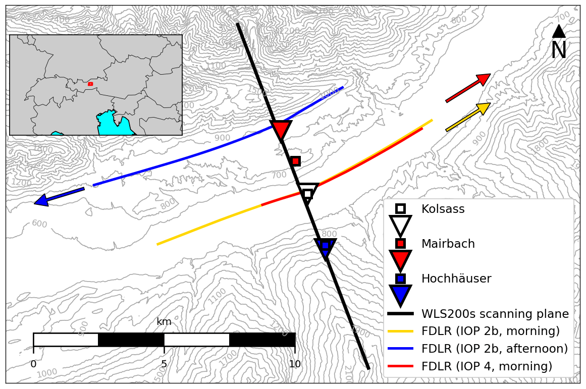
Figure 1 Overview map of the investigation area, centred around the Kolsass site at the Inn Valley floor. The square symbols indicate the locations of the permanent i-Box flux towers labelled with respect to their official designation (CS – core site; VF – valley floor; NF – north-facing; SF – south-facing; digit – local slope angle), while triangles denote the temporary KITcube WLS200s Doppler lidar locations. The solid black line represents the vertical plane of the coplanar-retrieved wind field. The three coloured solid lines represent the straight flight leg segments flown by the DLR Cessna aircraft during IOPs 2b and 4. Coloured arrows depict the direction in which the DLR Cessna aircraft flew the respectively coloured flight legs. The inset in the upper left corner denotes the location of the investigation area within Austria.

3 Investigation area, instrumentation, methodology

3.1 Site details

CROSSINN took place in the lower Inn Valley, approximately 18 km to the northeast of Innsbruck. The valley in this region is approximately 10 to 15 km wide crest to crest, roughly 1630 m deep (Adler et al., 2021d), while the valley floor is flat, in the cross-valley direction, for roughly 2 km (Fig. 1). The valley floor is dominated by a mixture of residential and cultivated areas, while the neighbouring valley sidewalls are mostly forested. The southern valley sidewall is characterized by a number of tributary valleys exiting nearly perpendicularly into the Inn Valley. Although the northern sidewall possesses no similar tributaries, it is characterized by a relatively flat, nearly 2 km wide plateau, extending approximately 300 m above the valley floor (AVF). The valley floor itself is located at an altitude of 546 m a.m.s.l. (MSL) in the investigation area.

3.2 Instrumentation details

We refer the reader to Adler et al. (2021d), their Table 3, as well as to B21, for a detailed overview of technical characteristics, scan types, and scan configurations concerning the remote sensing instrumentation. Here we focus on describing only a subset of the overall CROSSINN instrumentation of relevance for the present investigation. Note that all reported times are in UTC (local time LT = UTC+2).

3.2.1 WindCube Doppler lidars

Three WindCube WLS200s lidars, otherwise components of the KITcube measurement facility (Kalthoff et al., 2013), were deployed at three sites along a transect oriented in the cross-valley direction (Fig. 1). The reader can find the overview of the investigation area in Adler et al. (2021d) and B21. The accurate positioning of the three Doppler lidars, in an area of heterogeneous complex terrain, yielded three scanning planes which were offset by at most 120 m in the along-valley direction. The three lidars performed back-and-forth range height indicator (RHI) scans at an azimuth angle of 158.15°. The scanning region was chosen as a compromise between achieving a sufficiently large overlap region while still ensuring a fairly high temporal resolution between scans. As such, each RHI scan lasted 1 min, providing radial velocity v_r, carrier-to-noise ratio (CNR), and Doppler spectrum broadening at a physical resolution of 100 m, with overlapping range gate distance of 50 m, and a temporal resolution of 0.25 s. For more insight into the post-processing of these RHI scans, we refer the reader to B21.

3.2.2 Flux towers

The siting of CROSSINN instrumentation was primarily influenced by the locations of the long-term i-Box flux towers (Rotach et al., 2017). Specifically, the three flux towers of interest for the present study were CS-VF0, CS-SF1, and CS-NF27, where CS stands for “core site”, VF for “valley floor”, and NF and SF for “north-facing” and “south-facing”, respectively, and the digit represents the local slope angle in degrees. These three sites will in order hereafter be referred to as Kolsass, Mairbach, and Hochhäuser. More details concerning these sites and the data post-processing procedure can be found in Stiperski and Rotach (2016), B21, and Lehner et al. (2021). For this study we have chosen to select horizontal wind speed and direction (8.7 m a.g.l.) only at the CS-VF0 (Kolsass) site, while the surface sensible heat flux from all three sites will be used to distinguish unstable from stable ABL states. We refer the reader to Rotach et al. (2017) for more details concerning the setup of each of these three sites.

3.2.3 Radiosoundings

GRAW DFM-09 radiosondes were launched at discrete times from Kolsass to provide highly resolved in situ measurements of base thermodynamic variables during the four IOPs examined in this study. The temporal resolution of each sounding was 2 s, resulting in an average height interval of approximately 5–10 m. For a complete overview of each IOP and exact launch times, we refer the reader to Adler et al. (2021d), their Fig. 3.

3.2.4 Aircraft measurements

The Cessna 208 B Grand Caravan (D-FDLR) (German Aerospace Center, DLR) performed four along-valley flights during both IOPs 2b and 4 (Adler et al., 2021d; B21). The aircraft sampled in situ measurements of all three wind speed components, temperature, and specific humidity at a sampling rate of 100 Hz, with the METPOD sensor assembly (Mallaun et al., 2015). We analyse the flight legs flown at various levels within developing CBLs to validate features in the spectrum width sampled by the three WindCube lidars that are reminiscent of convection. Figure 1 illustrates the orientation of each analysed along-valley flight leg segment.

3.3 Methodology

3.3.1 Coplanar retrieval method

The focus of the CROSSINN campaign was the study of cross-valley flow, via the application of the coplanar retrieval method, known also as the dual-Doppler method (Calhoun et al., 2006; Hill et al., 2010; Newsom et al., 2015; Whiteman et al., 2018a, b; Wildmann et al., 2018; Peña and Mann, 2019; Adler et al., 2020, 2021d; B21; Haid et al., 2020, 2022; Wittkamp et al., 2021). During CROSSINN, this type of a retrieval method was applied to overlapping RHI scans performed by the three Doppler lidars. The alignment of the three RHI scans from each Doppler lidar, along with their synchronized start and end times, made it possible to retrieve v_v, the two-dimensional projection of the three-dimensional wind field onto a vertical cross-section. In this study, retrievals of v_v are performed onto a 8 km wide and 5 km tall Cartesian mesh with a lattice width Δl equal to 50 m (Adler et al., 2021d; B21). The retrieved v_v is rejected whenever the intersection angle of the original lidar beams was outside of the interval [30°, 150°], simultaneously for all three lidar pairs, resulting in regions with no cross-valley wind information near the Inn Valley sidewalls. Such a wide elliptical region has been discarded due to potentially large uncertainties of v_v owing to a near co-linearity of each lidar beam pair. In the present study we will only use the vertical wind speed component of the retrieved v_v wind field, denoted hereafter as w.

3.3.2 Spectrum width post-processing, merging, and evaluation

Turbulent Doppler spectrum broadening ${\mathit{\sigma }}_{\mathrm{t}}^{\mathrm{2}}$ can be defined as follows (Smalikho et al., 2005; Wildmann et al., 2019):

$$\begin{array}{}\text{(3)}& {\mathit{\sigma }}_{\mathrm{t}}^{\mathrm{2}}={\mathit{\sigma }}_{\mathrm{sw}}^{\mathrm{2}}-{\mathit{\sigma }}_{\mathrm{0}}^{\mathrm{2}}-{\mathit{\sigma }}_{\mathrm{s}}^{\mathrm{2}}-E,\end{array}$$

where ${\mathit{\sigma }}_{\mathrm{sw}}^{\mathrm{2}}$ is the measured spectrum width, ${\mathit{\sigma }}_{\mathrm{0}}^{\mathrm{2}}$ equals the spectrum width at constant wind speed within the sampling volume, ${\mathit{\sigma }}_{\mathrm{s}}^{\mathrm{2}}$ is the spectrum width due to shear effects, and E is the random error. During CROSSINN, no raw spectra data were stored primarily due to limitations in data storage capacity. Therefore, we resort to the spectrum width values, as outputted by the WLS200s internal software package Windforge. Although these products have ${\mathit{\sigma }}_{\mathrm{0}}^{\mathrm{2}}$ accounted for, they have not been corrected for shear effects and random errors (Ludovic Thobois, personal communication, 2021). As we will demonstrate in the following sections, this incompleteness does not affect the bulk contrasts between turbulent air within the CBL and less turbulent air aloft. Since the post-processing of these output spectrum widths requires a different set of criteria for removal of bad data than that for radial velocities (B21), in the following we describe these steps in more detail.

The interested reader is referred to the Supplement document, where the post-processing of spectrum width is described in more detail. Additionally, the Supplement contains the procedure for calibrating the bottom-up exceedance threshold method with the bulk Richardson number R_B approach. Upon a completed cycle of post-processing steps applied to each of 1 min RHI scan from each of the three WindCube lidars, merging together of all three scans is performed to obtain the final 1 min spectrum width snapshot used in the remainder of the study. We focus only on the region between the Hochhäuser and Mairbach Doppler lidars. Finally, owing to the post-processing steps described in more detail in the Supplement, we will hereafter denote the magnitude of spectrum width in arbitrary units (a.u.).

3.4 Validation of spectrum width against vertical velocity

Depicted in Fig. 2a is an early afternoon period on IOP 4, one of the most convective days sampled during CROSSINN. The developing CBL was characterized by intense surface-driven convection and weak along-valley flow (B21, their Fig. 8c). Note that the CVV has not yet begun to form at this time of day (B21). At this moment, the CBL was characterized by two narrow thermal updraughts, located approximately 1700 m south and 1100 m north of Kolsass, respectively, both reaching roughly 1000 m AVF. Unfortunately, there is no vertical velocity information close to the surface, due to the intersection angle region constraint explained earlier (Sect. 3.3.1). Lack of vertical wind information there discourages any worthwhile investigation of CBL evolution, especially during morning hours when convective features are shallow.

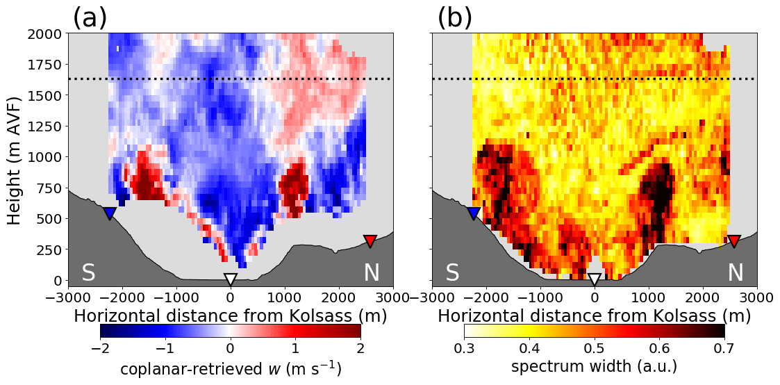
Figure 2 Instantaneous two-dimensional representation of (a) the coplanar-retrieved vertical velocity w and (b) the averaged merged corrected spectrum width field from the three WLS200s lidars, valid for 10:58 UTC on IOP 4. Spectrum width is expressed in arbitrary units (a.u.). Coloured triangles denote the locations of the WLS200s lidars visible in Fig. 1. The horizontal dotted black line indicates the altitude of the average ridgeline level equal to 1630 m above valley floor (AVF). White-coloured “N” and “S” denote the rough north-to-south alignment of the cross-valley transect, respectively.

This disadvantage of the coplanar retrieval methodology can be overcome by considering the merged spectrum width field in addition to the vertical wind (Fig. 2b), since this is derived directly from the RHI scans. At first glance, the similarity between the shape and location of elevated spectrum width regions and the updraughts (Fig. 2a) is striking. More importantly, Fig. 2b demonstrates that the two updraughts were both attached to the surface, a characteristic one cannot infer from Fig. 2a. Nonetheless, one must keep in mind that the lidar cross-valley transect is also sampling such convective features as they get advected through the investigation area. For instance, a convective structure being advected by the along-valley flow could therefore, despite its expected lifetime of 5–10 min in a well-developed convective environment, pass through our transect over a much shorter period of time. As a result, instances of low turbulent regions capped by more turbulent air, such as the one over the plateau about 2000 m north of Kolsass, suggest a transient, non-locally generated thermal detached from the plateau. Similarly, the thermal in question may still be attached to the plateau but simply vertically tilted. As a result, inferring instantaneous CBL depths for such cases, as opposed to a temporal averaging approach where for instance hourly averages are computed, may be misleading. Keeping in mind that the showcased spectrum width field was previously manipulated during post-processing (Sect. 3.3.2), it is nonetheless clear that the turbulence levels within the two updraughts (greater than 0.7 a.u.) were nearly double in magnitude compared to the upper valley atmosphere (predominantly 0.45 a.u.). We observed background values outside of the boundary layer rarely to drop below 0.38 a.u. (not shown). This contrast between surface-driven convection adjacent to the surface and low-turbulence regions aloft, as inferred from spectrum width variability in space, lends itself as a tentatively useful tool for tracking the CBL evolution in both time and space.

3.5 Comparing features in spectrum width and vertical velocity

The calibration of the bottom-up method with the R_B method (see Supplement), despite being a success, left the representativity of the cross-valley transect with respect to the rest of the investigation area unaddressed. Additionally, it remains unclear whether instantaneous, 1 min spectrum width features, such as the turbulent thermals visible in Fig. 2b, can indeed be equated with regions of convectively driven turbulence. Given the lack of systematic and routine in situ measurements of turbulence parameters other than at the surface, this validation cannot be performed in a manner similar to the radiosondes earlier. Fortunately, the DLR Cessna aircraft flew a number of flight legs both inside and outside of the CBL on IOPs 2b and 4 (Fig. 1) while sampling at a sufficiently rapid rate to allow a robust computation of spatio-temporal averages (Table 1). We will explore three different flight legs flown at various stages of CBL development: (i) a late morning flight leg flown near the top of a shallow CBL on IOP 2b (Fig. 3a), (ii) a late morning flight leg flown within a more turbulent and relatively deeper CBL on IOP 4 (Fig. 3b), and (iii) a late afternoon flight leg flown slightly above an apparently mature CBL on IOP 2b (Fig. 3c), given the time of day when the leg was flown. To assess the turbulent state and fidelity of corresponding spectrum width features through which the aircraft flew, we will consider the in situ perturbations of vertical velocity w^′ (Fig. 4a–c), potential temperature θ^′ (Fig. 4d–f), specific humidity q^′ (Fig. 4g–i), and instantaneous kinematic heat flux $w^{\prime }{\mathit{\theta }}^{\prime }$ (Fig. 4j–l) and instantaneous kinematic moisture flux $w^{\prime }{q}^{\prime }$ (Fig. 4m–o). Perturbations are computed as linearly detrended values only for the straight leg segments. The standard deviation of the aircraft height along the straight leg segment amounted to 2, 9, and 6 m, while the average aircraft velocity equaled 68, 63, and 66 m s⁻¹, for each of the three flights, respectively. Although the horizontal leg segments were slightly curved to account for the valley curvature in this part of the Inn Valley (Fig. 1), we nonetheless assume a negligible impact of aircraft turning on the quantities scrutinized here, considering we do not focus on horizontal velocity components.

Table 1 Vertical velocity variance $\langle {w^{\prime }}^{\mathrm{2}}\rangle$, kinematic sensible heat flux $\langle w^{\prime }{\mathit{\theta }}^{\prime }\rangle$, and kinematic latent heat flux $\langle w^{\prime }{q}^{\prime }\rangle$, for the three selected flights on IOPs 2b and 4 (Figs. 3, 4). Angle brackets indicate spatio-temporal averages computed as an average of the entire straight leg segment flown along the valley. Turbulence perturbations are computed as deviations from a linear trendline.

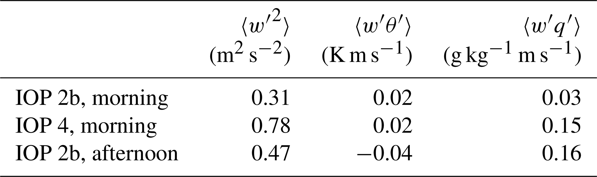
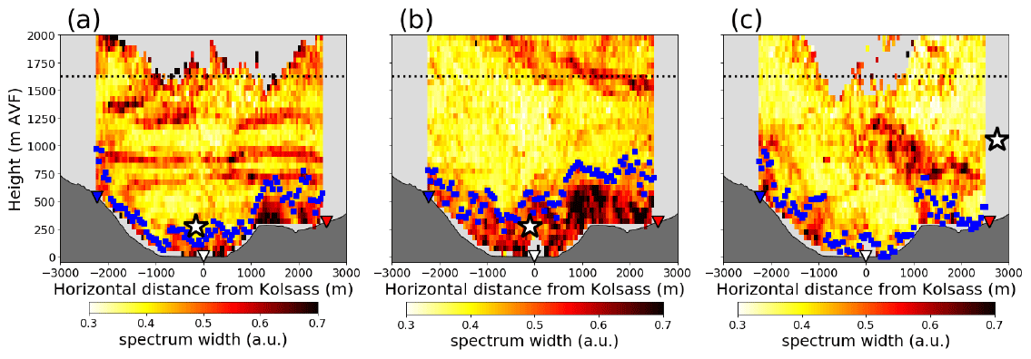
Figure 3 Instantaneous spectrum width fields during the times when the along-valley flight legs were flown closest to the WLS200s cross-valley transect, at (a) 08:26 UTC on IOP 2b, (b) 09:36 UTC on IOP 4, and (c) 14:20 UTC on IOP 2b. The blue squares represent the z_i obtained by applying the bottom-up method to the 1 min corrected spectrum width fields, averaged across the duration of each straight flight leg segment. The white stars denote the flight leg position, while the coloured triangles and the horizontal dotted black lines are as in Fig. 2. Orientation of the cross-valley transect is the same as in Fig. 2.

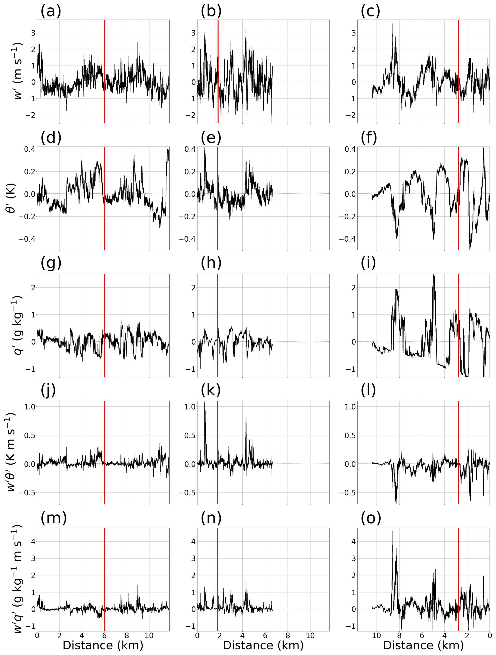
Figure 4 Along-valley, 100 Hz flight leg measurements made by the METPOD package aboard the DLR Cessna aircraft of (a, b, c) vertical velocity perturbations w^′, (d, e, f) potential temperature perturbations θ^′, (g, h, i) specific humidity perturbations q^′, (j, k, l) $w^{\prime }{\mathit{\theta }}^{\prime }$, and (m, n, o) $w^{\prime }{q}^{\prime }$. Shown are time periods corresponding to (a, d, g, j, m) 08:24:25–08:27:15 UTC on IOP 2b, (b, e, h, k, n) 09:35:40–09:37:25 UTC on IOP 4, and (c, f, i, l, o) 14:19:15–14:21:50 UTC on IOP 2b. The three flight legs were flown at average heights of 250, 250, and 1400 m AVF, respectively. The red lines denote the locations of the lidar cross-valley transect. The horizontal axis limits in (b, e, h, k, n) and (c, f, i, l, o) have been extended to match the longest leg segment in (a, d, g, j, m). Note that the x axis for the rightmost flight leg is reversed since this leg was flown in an opposite direction compared to the rest (Fig. 1). Nonetheless the east–west orientation in each subplot shown here is universal.

We begin with the late morning flight performed on IOP 2b, with the relevant straight leg segment flown between 08:24 and 08:27 UTC at an average altitude of approximately 270 m AVF (Figs. 3a, 4). Unlike the example introduced by Fig. 2, the valley atmosphere lacked any vigorous and deep thermal activity at this time, with most of the surface-driven convection situated above the plateau. Furthermore, three layers of elevated spectrum width are found at heights of approximately 700, 900, and 1250 m AVF, most likely due to wind shear present in the downvalley flow at this time (B21, their Fig. 8a). Since the aircraft flew at a height where, based on spectrum width magnitude, turbulence intensity was fairly weak, we can expect to observe weak perturbations and covariances sampled by the aircraft. Indeed, the majority of the most vigorous w^′ and q^′ were concentrated between the 6th and 10th kilometre of the segment (Fig. 4a, g), resulting in peak positive $w^{\prime }{q}^{\prime }$ there as well (Fig. 4m). On the other hand, the most energetic θ^′ perturbations were associated with mesoscale gradients, evident by the distinct jump between the second and sixth kilometre of the segment (Fig. 4d). Nonetheless, the positive signs of both $w^{\prime }{\mathit{\theta }}^{\prime }$ and $w^{\prime }{q}^{\prime }$ agree with the textbook expectancy of these covariances to be positive inside the CBL (Stull, 1988; Moeng and Sullivan, 1994; Schmidli, 2013; Wulfmeyer et al., 2016), suggesting that the aircraft has indeed flown through the CBL but may not have remained within it for the entire duration of the segment.

Having been flown at an average elevation of 263 m AVF, the aircraft encountered markedly stronger turbulence levels during the late morning flight on IOP 4, between 09:35 and 09:37 UTC (Figs. 3b, 4). As a result, the vertical velocity perturbations w^′ shown in Fig. 4b were larger than on IOP 2b (Fig. 4a), with more equidistant perturbations of the same order of magnitude between −2 and 3 m s⁻¹. Although the ranges of θ^′ and q^′ were comparable to those on IOP 2b, they corresponded to a greater degree to the w^′ features, therefore resulting in larger magnitudes of the respective covariances as well (Fig. 4k, n; Table 1). In particular, the fairly regular positive $w^{\prime }{q}^{\prime }$ excursions between kilometres 0 and 6 suggest nearly equidistant ejections of moist air from the surface layer to the level of the flight leg. Overall, the more turbulent state of the CBL on IOP 4 is also reflected in the vertical velocity variance $\langle {w^{\prime }}^{\mathrm{2}}\rangle$ values being more than double in magnitude of those on IOP 2b (Table 1). Despite this leg having been flown a little over an hour later than on IOP 2b, the positive signs of both $\langle w^{\prime }{\mathit{\theta }}^{\prime }\rangle$ and $\langle w^{\prime }{q}^{\prime }\rangle$ once again confirm the leg was flown within the CBL.

To ascertain whether the spectrum width approach of studying the CBL is viable not just for developing CBLs, but also in the case of mature ones, we also explore the third flight leg, having taken place on late afternoon of IOP 2b, between 14:19 and 14:21 UTC at an average altitude equal to 1084 m AVF (Figs. 3c, 4). Characterized by low turbulence levels over the valley floor, most of the supposedly non-locally generated turbulence at this time occurred above the plateau, between 500 and 1100 m AVF (Fig. 3c). However, there seems to have been a disconnect between the turbulence in the surface layer above the plateau between 1000 and 2000 m north of Kolsass and those higher turbulence regions aloft. Taking into account that the upvalley flow at this time was stronger than the downvalley flow 6 h earlier (Fig. 3a), we conclude that in the case of sufficiently tall thermals in a mature CBL, their advection by the mean wind through the lidar transect should be an important factor to consider. Furthermore, given the fact that the flight leg was located near the upper boundary of most turbulent thermals, we should not expect to encounter similar relationship in signs of the covariances compared to the two flight legs examined earlier (Fig. 3a, b). Since the leg was flown in the vicinity of a mature CBL, the perturbations w^′, θ^′, and q^′ (Fig. 4c, f, i) reflect evidence of thermals, specifically four discrete ejections ($w^{\prime }>\mathrm{0}$) of potentially colder (${\mathit{\theta }}^{\prime }<\mathrm{0}$) and moister ($q^{\prime }>\mathrm{0}$) air from the CBL to the level of the aircraft. In Fig. 4c, f, and i these four signatures may be found approximately at kilometres 2, 4, 5, and 8, respectively. This is particularly evident from the deviations of the specific humidity from ambient, upper-valley levels of humidity. As a result, $w^{\prime }{\mathit{\theta }}^{\prime }$ at the locations of the four discrete thermals is primarily of negative sign (Fig. 4l), while $w^{\prime }{q}^{\prime }$ is primarily of positive sign (Fig. 4o). Spatio-temporal averages of these two covariances (Table 1) reflect this relationship between the two, suggesting that the aircraft most likely flew within the CBL entrainment zone or slightly above it, due to the negative sign of $\langle w^{\prime }{\mathit{\theta }}^{\prime }\rangle$ (Stull, 1988; Wulfmeyer et al., 2016). Lastly, the presence of such discrete thermals along the entire leg, spaced fairly evenly apart, suggests that the entire plateau supported a similar CBL structure, fortifying the representativeness of our single cross-valley lidar transect.

4 Spatio-temporal determination of MoBL behaviour in the investigation area

Having calibrated the bottom-up method to accommodate the range of conditions specific to the Inn Valley during summertime, as well as adequately validated the spectrum width features with in situ measurements, in the remainder of the study we focus our attention on four IOP events (Adler et al., 2021d): IOPs 2a (8 August), 2b (9 August), 3 (11 August), and 4 (14 August). These successional IOPs have several favourable characteristics which help us minimize the degrees of freedom of the research questions listed in Sect. 1. First, they span a single week, from 8 to 15 August, therefore allowing us to disregard seasonality and, by extension, possible changes in varying sensible and latent heat fluxes between the IOPs. Second, none of the four IOPs experienced prolonged periods of cloud cover during daytime, which would have, due to their intermittency, made heat flux comparisons more difficult and inhibited lidar measurements. However, with the exception of IOP 2b, all other IOPs experienced moderate amounts of low and mid cloud cover during night (Adler et al., 2021d, their Fig. 5d), disrupting the long-wave radiative losses before sunrise and thus helping explain some of the differences between observed sensible heat fluxes among the four IOPs as well as the lack of more regular downvalley flow during night (Fig. 5). Third, they took place within a time window short enough to allow us to assume a stationary state of the land use in the investigation area, thus constraining the regional relationships between sensible and latent heat fluxes driving the MoBL. Fourth, these IOPs experienced a substantial range of different large-scale forcings, permitting us to gain deeper insight into different mechanisms affecting CBL structure (Adler and Kalthoff, 2016; Weinkaemmerer et al., 2022). All four IOPs were accompanied by moderately strong southwesterly flows above the Alps (B21, their Fig. 4). The most pronounced synoptic influence was present on IOPs 2b and 3. As a result, the fairly weak night-time downvalley flow on IOP 2b persisted longer into the afternoon compared to other IOPs (Fig. 5), while the second half of IOP 3 was marked by an intense foehn episode which gradually reached the lower portions of the valley in the evening. The valley floor experienced weak and intermittent rainfall during the first few hours of IOP 4, until approximately 06:00 UTC (Adler et al., 2021d, their Fig. 5e).

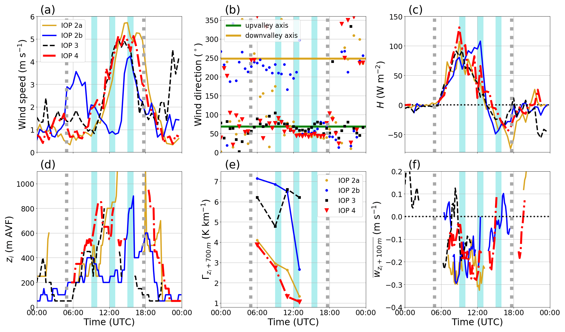
Figure 5 Time series of (a) wind speed at 8.7 m a.g.l. at Kolsass, (b) wind direction at 8.7 m a.g.l. at Kolsass, (c) sensible heat flux H at 8.7 m a.g.l. at Kolsass, (d) local z_i above Kolsass, (e) mean lapse rate for the 700 m thick layer above local z_i above Kolsass from the temperature T calculated from radiosonde data, and (f) mean coplanar-retrieved vertical velocity w within a 100 m thick layer above local z_i above Kolsass, for the four IOPs shown in Fig. 6. The three shaded orange regions denote the respective 1 h windows shown in Fig. 7. The two vertical grey bars denote respectively the local sunrise (04:54 UTC) and sunset (17:40 UTC) times on 11 August 2019.

4.1 Temporal variability of parameters impacting CBL development

We first explore the evolution of traditional parameters involved in studying CBL growth development. We focus on examining near-surface conditions at the valley floor only, with the aim of characterizing the along-valley wind, the observed z_i variability, and of relating this variability to the temporal evolution of terms in Eq. (2). Due to the surrounding ridges, on the day of IOP 3 (11 August) Kolsass experienced local sunrise and sunset at approximately 04:54 and 17:40 UTC, respectively. In the analyses to follow, we will assume that these times were valid for the entire considered week.

As established recently in B21, the pattern of near-surface wind evolution at the floor of the Inn Valley exhibited typical diurnal trends (Whiteman, 2000; Zardi and Whiteman, 2013), namely the prevalence of downvalley flows at night and relatively stronger upvalley flows at day (Fig. 5a, b). However, of the four targeted IOPs, only IOP 2b exhibited a pronounced morning downvalley flow. This deviation of IOP 2b during nighttime could be due to synoptic foehn influence, as the foehn probability diagnostic (Plavcan et al., 2014) indicated a high probability of foehn on this day (Adler et al., 2021d, their Fig. 5c). During daytime, all IOPs experienced an upvalley flow but to varying extents. While the strongest and longest upvalley flow took place on IOP 2a, a weaker upvalley flow with a later than usual onset occurred on the following day, during IOP 2b. Daytime upvalley flows typically began around 10:00 UTC, ceasing fully by 21:00 UTC. These time frames correspond to the previously determined CVV durations (B21). Fully developed CVVs spanning the entire valley depth were present only on IOPs 2a and 4. Although IOP 3 based on Fig. 5 seems to have behaved in a manner similar to other IOPs, following analyses will prove how consideration of only near-surface parameters may often be misleading when it comes to complex terrain flows. As expected, the sensible heat flux for all IOPs (Fig. 5c) similarly became positive at approximately 05:30 UTC while changing sign again fairly early compared to local sunset, around 13:30 UTC. Such an early sign change is a result of relatively larger latent heat fluxes in the Inn Valley, owing to cultivated land use and patchy forested regions (Lehner et al., 2021). While IOPs 2a, 3, and 4 exhibited the highest sensible heat fluxes at 09:00 UTC of around 100 W m⁻², IOP 2b stood out, as its peak value occurred somewhat later at 12:30 UTC, for which we hypothesize that the foehn influence may have sufficiently altered the otherwise expected behaviour of energy partitioning near the surface of the Inn Valley.

Next we turn our attention to the CBL development, initially above Kolsass only. Starting at approximately 06:00 UTC, the CBLs gradually deepened but with varying growth rates (Fig. 5d). By 13:00 UTC, IOP 2b has evidently established itself as a shallow CBL case, not exceeding 300 m in depth. On the other hand, CBLs during the other three IOPs reached approximately 800 to 1200 m AVF. Such a CBL growth behaviour corresponded fairly well with the prevalent positive sign of the sensible heat flux H at Kolsass between 06:00 and 13:00 UTC (Fig. 5c). After 13:00 UTC, the z_i estimates among the IOPs diverged considerably. Interestingly, despite the intermittent rain on the night and early morning of IOP 4, some of the deepest CBLs during CROSSINN were found exactly on IOP 4, driven by more intense convection relative to the other three IOPs. Some inconsistencies have arisen, for instance the shallowest z_i despite the largest H on IOP 2b between 11:00 and 13:00 UTC. To offer an explanation for this, we consider next the two opposing factors of simplified one-dimensional CBL growth (Eq. 2), namely stability Γ and subsidence w_L.

Upper-level stability $\mathrm{\Gamma }=\mathrm{\Delta }\mathit{\theta }/\mathrm{\Delta }z$ was computed for the radiosonde launches between 06:00 and 13:00 UTC, as the lapse rate in a 700 m deep layer above the local z_i above Kolsass at the time of launch. Experimenting with various layer thicknesses offered no evidence of change of the dominant Γ tendencies with time (not shown). The 06:00 UTC launches, conducted shortly after sunrise, were included, given the fact that CBL growth models take Γ as an initial condition while also assuming it remains constant over the course of the day. As clearly depicted by Fig. 5e, this assumption is violated in the Inn Valley because the layer above the CBL is still a part of the MoBL. Rather, the free tropospheric stability, above approximately 3000 m AVF, was observed to remain steady during daytime on all IOPs (not shown), suggesting that the influence of the MoBL at the Alpine scale may cease beyond 3000 m AVF. One possible explanation for the overall shallowest CBL encountered on IOP 2b could be the largest 06:00 UTC stability Γ of nearly 7 K km⁻¹, even more so since, unlike the other three IOPs, particularly IOPs 2a and 4, Γ on IOP 2b remained fairly high until 11:00 UTC. On the other hand, the deeper CBLs on IOPs 2a and 4 (Fig. 5d) experienced less resistance during their deepening, by growing into progressively less stable air aloft, as indicated by their Γ values decreasing from roughly 4 to 1 K km⁻¹. During IOP 3, Γ stayed fairly constant in the range 4.5–6.5 K km⁻¹ (Fig. 5e). However, it did not exhibit a typical decrease over the course of the day as was the case with the other three IOPs.

Lastly, we aim to establish the main temporal characteristics of subsidence w_L, here calculated as the average coplanar-retrieved vertical velocity in a layer 100 m thick directly above local z_i above Kolsass (Fig. 5f). Although subsidence values exhibit large variability among the IOPs, they do not exhibit any consistent trend during daytime, with strongest subsidence reaching −0.25 m s⁻¹ on average. Despite being based on 1 h averages, these w_L are still larger than typical subsidence values encountered over flat, horizontally homogeneous terrain (Avissar and Schmidt, 1998; Blay-Carreras et al., 2014; Pietersen et al., 2015), even over a single mountain range (Kalthoff et al., 1998; Kossmann et al., 1998). Subsidence values of the order of magnitude found in the observations shown here correspond to the ones encountered in highly resolved daytime valley flow simulations conducted by Serafin and Zardi (2011). Interestingly, between approximately 07:00 and 10:00 UTC, both IOPs 2a and 2b experienced comparably intense subsidence, between −0.2 and −0.3 m s⁻¹. During this time frame, both H and z_i between the two IOPs behaved similarly as well. After 10:00 UTC the CBLs on these two IOPs began to diverge in depth, suggesting that after 10:00 UTC, the far more stable air above the CBL on IOP 2b was the main factor opposing the CBL growing any deeper than 300 m. It is important to emphasize that the deeper turbulent boundary layer found later on IOP 2b, specifically at 16:00 UTC with a depth of 900 m, took place during time when the sensible heat flux at the surface already became negative (Fig. 5c). In the remainder of the study, we will refer to these afternoon boundary layers, due to the broad variety of the origin of their turbulence, simply as a turbulent boundary layer, rather than the MoBL, which we are not sampling entirely. As shown by theoretical derivations performed by Ouwersloot and Vilà-Guerau de Arellano (2013b), the effects of stability and subsidence do not add linearly, demonstrating that the effect of subsidence becomes more pronounced with weaker stability (Ouwersloot and Vilà-Guerau de Arellano, 2013a). This seems to have been the case for IOP 2a only until 10:00 UTC or so, after which the CBL suddenly gained depth despite a stronger subsidence around 12:00–13:00 UTC than previously (Fig. 5f). Once again we emphasize the high probability of foehn on IOP 2b, hinting at a possible inability of our bottom-up method to differentiate between convectively driven turbulence and shear-induced turbulence (owing to the likely presence of foehn at this time) as was the case in this IOP. Based on Fig. 5 we hypothesize that upper-valley stability Γ may serve as the primary factor opposing CBL growth. Additionally, it is important to note that subsidence in complex terrain often results from horizontal convergence of upslope flow branches detaching from the slopes (Schmidli, 2013; Adler and Kalthoff, 2014; Serafin et al., 2018), in addition to large-scale weather patterns. Admittedly, subsidence on IOP 2b may have also been to some extent affected by the foehn. Furthermore, although not synoptically generated, subsidence induced by mountain–plain–wind circulation penetrating deeper into the Alps during late afternoon could also have played a role in all IOPs (Lugauer and Winkler, 2005; Goger et al., 2019, their Fig. 7). However, differentiating to what extent these additional factors contributed to subsidence during these four IOPs is out of the scope of the present study. We also emphasize once again our neglect of horizontal effects on z_i tendency in Eq. (1), which we have not been able to infer from existing measurements.

4.2 Time–height evolution of spectrum width, potential temperature θ, and CBL depth z_i

Figure 6 includes R_B-based z_i estimates for the radiosondes launched between 06:00 and 15:00 UTC, whenever a z_i estimate was provided by the R_B method, and also z_i obtained using the bottom-up approach applied to spectrum width. The lack of data during early morning hours on IOPs 2a and 4 is due to overcast conditions (Fig. 6a, d). The sporadic data gaps below 200 m AVF are due to the dead zone of the lidar at Kolsass. Since the lidar at Hochhäuser was scanning with negative elevation towards Kolsass, spectrum width data available occasionally within this layer indicate valid data originating from the Hochhäuser RHI measurements.

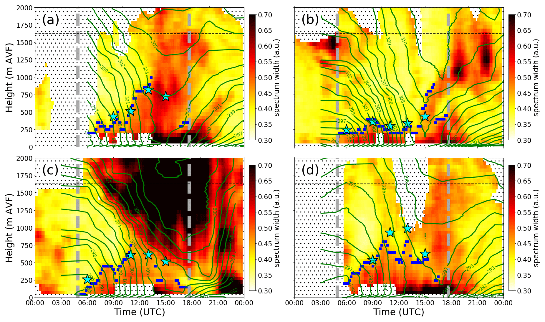
Figure 6 Time–height representation of spectrum width for the column above Kolsass (shading), radiosonde isentropes (green contours), z_i obtained using the bottom-up threshold approach applied to spectrum width (blue squares), and z_i obtained using the bulk Richardson method (cyan stars), for (a) IOP 2a, (b) IOP 2b, (c) IOP 3, and (d) IOP 4. The z_i values obtained using the bottom-up threshold approach are omitted for nighttime periods, as the method was not calibrated to perform well during shallow stable boundary layer conditions. Each shaded spectrum width column is based on hourly windows shifted forward in time by 10 min for enhanced visual detail. The horizontal dashed black lines are as in Fig. 2, while the vertical dashed grey bars are as in Fig. 5. Hatched regions denote absence of available spectrum width data. To generate contour lines for the isentropes, all radiosonde launches from each IOP were used.

In agreement with Fig. S4 in the Supplement, z_i estimates derived using the bottom-up approach on IOPs 2a and 2b showed decent agreement with those stemming from the R_B method (Fig. 6a, b). The agreement between the bottom-up and R_B methods holds well for IOP 3 too; however in the case of the 11:00 and 13:00 UTC radiosondes on IOP 4, the R_B method yielded systematically deeper CBLs. Further corroboration of the bottom-up approach is provided when considering the angle of the isentropes between 08:00 and 14:00 UTC on all IOPs, with more vertical isentropes present inside of the CBL compared to more slanted isentropes aloft. Undoubtedly, IOP 3 stands out due to the growing influence of a deep, highly turbulent layer descending into the Inn Valley over the course of the day. This is due to the intensifying southerly to southwesterly foehn, associated with strong shear effects, near-neutrally stable atmosphere, and intense mountain wave breaking, leading even to rotors (Adler et al., 2021d, their Fig. 4). However, the descending foehn layer on IOP 3 not only suppressed the CBL growth, as indicated by the R_B-based z_i, but also it limited the depth of the evolving upvalley flow, thus inhibiting the formation of a well-developed CVV found on otherwise more quiescent IOPs 2a and 4 (B21).

After roughly 14:00 UTC on IOP 2a (Fig. 6a) and 15:00 UTC on IOP 4 (Fig. 6d), turbulence spread through the entire valley atmosphere, as indicated by the abrupt increase in spectrum width values of 0.5 a.u. on average. This corresponds to the presence of a CVV (B21). The shear character of the MoBL at this time is further supported by the presence of highest spectrum width values below 250 m AVF, in excess of 0.7 a.u., demonstrating the presence of a low-level upvalley jet, which is responsible for CVV occurrence. Extremely high values of spectrum width are related to significant turbulence shear production at this time of day, which results from large vertical wind shear $\mathrm{d}U/\mathrm{d}z$ in the layer below the jet maximum, and possibly also from significant momentum covariance $\stackrel{\mathrm{‾}}{u^{\prime }{w}^{\prime }}$ (Stull, 1988). It is worth noting that the performance of the bottom-up method becomes inferior in such a shear-dominated environment, given that the spectrum width does not at all cross the threshold previously designed for convectively driven situations only. On IOP 2b (Fig. 6b), the insufficiently weak upvalley flow yielded no CVV, while on IOP 3 (Fig. 6c) the development of a CVV was prevented by the gradual descent of the southern foehn into lower levels of the valley atmosphere.

Between 16:00 and 22:00 UTC on IOP 2a, for instance, during the time when the upvalley flow jet is decoupling from the surface (B21, their Fig. 8), the bottom-up approach is once again able to retrieve the depth of primarily shear-generated turbulent zones. However, this layer no longer possesses any meaningful connection to buoyantly driven turbulent layers, since the sensible heat flux H became negative several hours earlier (Fig. 5c). They are probably linked to the decay of the CVV, which appears to be rather non-uniform with height. An interesting occurrence began around 14:00 UTC on IOP 2b (Fig. 6b), when the gradual decoupling of higher spectrum width from the surface eventually settled at a height of approximately 1000–1400 m AVF. The bottom-up method erroneously identified this gradual rising layer as the CBL top, pointing to the necessity of carefully interpreting spectrum width layers and gradients when multiple sources of turbulence may occur. As the bottom-up method was not calibrated for these evening and nighttime periods (e.g. Fig. 6b), proper interpretation is mandatory.

To summarize, the previous two sections have demonstrated the useful capability of the bottom-up exceedance method for gaining insight into the evolution of the daytime MoBL in the CROSSINN investigation area. Particularly from sunrise until H sign reversal, the method enabled us to track the evolution of the growing and maturing CBL throughout the entire cross-valley transect. Unfortunately, similar diagnostic capabilities of this method were not applicable to the afternoon and evening periods once H reversed sign, CVV begun to fill up the valley atmosphere, or the south foehn descended sufficiently close to the valley floor to disrupt the formation of a residual layer or even stable boundary layer at this time. In other words, using spectrum width directly output by the lidar manufacturer, without decomposing ${\mathit{\sigma }}_{\mathrm{t}}^{\mathrm{2}}$ (Eq. 3) into its individual constituents, we were only able to rely on the bottom-up exceedance method during periods characterized by a quiescent growth of the CBL, when buoyancy was the governing turbulence production process.

4.3 Identifying distinct regimes of daytime MoBL spatial evolution

Previous conclusions made based on Figs. 5 and 6 suggested a complex evolution of the MoBL above the Inn Valley floor. In the following we define three distinct stages of MoBL evolution, during three identical time windows (09:00–10:00, 12:00–13:00, 15:00–16:00 UTC, indicated by the vertical shaded orange regions in Fig. 5), now also considering the spatial variability in the cross-valley transect. This characterization is once again enabled by the tight chronological succession of the four IOPs, allowing us to neglect seasonality and, by extension, varying daytime duration. Additionally, we highlight the fact that, although our treatment of the artificial oscillatory patterns in the RHI measurements from the Mairbach lidar was successful when considering instantaneous, 1 min snapshots (Fig. S3), the act of computing hourly averages of spectrum width teased out some remaining artefacts in the cross-valley transects (e.g. Fig. 7g, h, i, l). Since these situations occurred mostly during the later part of day when the performance of the bottom-up method is compromised anyway, it does therefore not affect our findings made for CBL states earlier during the IOPs.

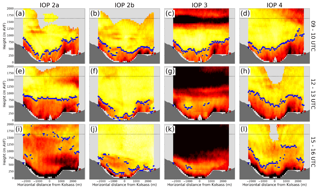
Figure 7 Cross-valley representations of 1 h averaged spectrum width starting at (a, b, c, d) 09:00 UTC, (e, f, g, h) 12:00 UTC, and (i, j, k, l) 15:00 UTC, for (a, e, i) IOP 2a, (b, f, j) IOP 2b, (c, g, k) IOP 3, and (d, h, l) IOP 4. Blue squares denote z_i obtained using the bottom-up threshold approach applied to each column of spectrum width. Coloured triangles and the horizontal dotted black lines are as in Fig. 2. The colourbar, omitted in favour of space, is identical to the ones found in Figs. 2, 3, and 6. Orientation of the cross-valley transect is the same as in Fig. 2.

Of all three time windows, the first one between 09:00 and 10:00 UTC (Fig. 7a–d) demonstrates the greatest degree of similarity across the IOPs. At this time, the along-valley flow is relatively weaker than later in the day (Fig. 5a), and the sensible heat flux is at its most intense (Fig. 5c), while the CBL growth rates among the IOPs are fairly comparable (Fig. 5d). Mostly terrain-following CBL top and an elevated spectrum width region fixed to the southern edge of the plateau denote the main characteristics of this regime. The former characteristic is a well-known property of morning CBLs in valleys (De Wekker and Kossmann, 2015), while the latter characteristic suggests highly turbulent upslope flows (Adler et al., 2021d, their Fig. 7c, d), in the form of thermals, detaching from the plateau owing to their inertia. An instantaneous detachment of a thermal from the plateau is evident in Fig. 2. Despite the developing foehn on IOP 3, at this point still limited to the ridgeline level, the CBL was nonetheless able to develop in a manner similar to the other IOPs (Fig. 7c). As far as sidewall contrasts are concerned, CBLs up to 200 m deeper above the plateau than over the southern sidewall are a common feature of all IOPs, with the exception of IOP 2b.

By 12:00 UTC (Fig. 7e–h), significant deviations in the CBL development have arisen. On the one hand, the upvalley flow is on average gaining in intensity (Fig. 5a, b), while on the other hand the sensible heat flux resumes to weaken, changing sign within the next hour (Fig. 5c). The cross-valley CBL structure among the IOPs has lost any degree of similarity present just 3 h ago (Fig. 7a–d). Of the four IOPs, only IOP 2a (Fig. 7e) has achieved one of possible textbook stages of CBL development in a valley, namely a level CBL top independent from terrain (De Wekker and Kossmann, 2015). On IOP 2b (Fig. 7f), the CBL has slightly deepened or at least remained constant over the slopes compared to the morning regime, while it became shallower over the valley floor, as shown already in Figs. 5d and 6b. The continually descending foehn layer on IOP 3 (Fig. 7g) has reached the undisturbed CBL by this time, resulting in the inability of the bottom-up method to yield meaningful z_i anymore. Interestingly, despite the overall similarity between IOPs 2a and 4 (Figs. 5, 6), the cross-valley CBL structure on IOP 4 retained its terrain-following structure. Lastly, it is noteworthy to mention that the plateau-locked upslope flows were still present at this time on all IOPs except IOP 2b, roughly with the same degree of turbulence intensities as 3 h prior. Although buoyancy still represents a driving mechanism at this time, increased shear via intensifying upvalley flow and varying synoptic influences have led to pronounced differences among the IOPs.

With the upvalley flow having reached its pinnacle between 15:00 and 16:00 UTC (Fig. 5a, b), in the face of a negative sensible heat flux (Fig. 5c), the turbulent boundary layer across all four IOPs entered a primarily shear-driven regime (Fig. 7i–l). The cross-valley spectrum width fields are largely characterized by the inadequacy of the bottom-up method in identifying the CBL top z_i on the one hand and by the uniform region of surface-attached high spectrum width, particularly on IOPs 2a and 4 (Fig. 7i, l). As noted earlier, this points to the low-level upvalley flow jet. Additionally, the elevated turbulence near the ridgeline level could also partly be due to penetrating mountain–plain–wind circulation at this time of day, as well as foehn in the case of IOPs 2b and 3 (Goger et al., 2019).

To summarize, despite having started from a state of textbook-like, terrain-following CBL structure during the morning (Fig. 7a–d), the CBL during each IOP experienced a substantially different structure by late afternoon (Fig. 7i–l), depending primarily on the temporal evolution of upvalley flow, upper-valley stability, presence of foehn, and tentative penetration of a mountain–plain–wind circulation. As a result, the structure of the turbulent boundary layer in the early evening period differed drastically among the four IOPs.

4.4 Cross-valley variability of MoBL evolution

Highly spatio-temporally resolved fields of CBL depth z_i are readily available from modelling tools such as idealized large eddy simulations (LESs). A common visualization technique for analysing such fields is a time–distance Hovmöller-style diagram, as found for instance in Catalano and Moeng (2010), their Fig. 7, or in Schmidli (2013), his Fig. 1b. Obtaining such detailed spatial information of z_i evolution routinely in time from observations remains a substantial challenge to overcome. To our knowledge, we report z_i for the first time from observations in such a Hovmöller-style fashion (Fig. 8). This novelty is further augmented, by also considering the evolution of subsidence in both space and time, which together with the inclusion of Γ and H enables a unique glance into CBL evolution (Eq. 2). Note that the z_i reported in Fig. 8 is now in m a.g.l. instead of m AVF used so far. In the following, we analyse IOP 2a in more detail while only pointing out similarities and differences on the other IOPs compared to IOP 2a.

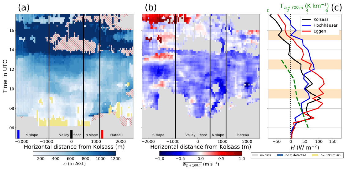
Figure 8 (a) Distance–time representation of z_i (now in m a.g.l) obtained using the bottom-up threshold approach applied to each cross-valley column of spectrum width (shading), with additional indicators for no estimation possible (grey shading), for no z_i detected (hatching) and for z_i shallower than 100 m a.g.l. (in yellow), (b) distance–time representation of the mean coplanar-retrieved vertical velocity w within a 100 m thick layer above local z_i, and (c) time series of sensible heat flux H from the three i-Box stations (in legend), together with the lapse rate for the 700 m thick layer above local z_i above Kolsass from the radiosonde potential temperature θ (in green). Shown is IOP 2a. The vertical lines in (a, b) denote borders of the major terrain features in the valley cross-section (S slope – southern slope; N slope – northern slope), while the short coloured bars on the bottom correspond to the locations of the respective i-Box sites. The vertical axis has been constrained to the time between local sunrise and sunset.

As before (Figs. 5d, 6), we applied the bottom-up method to 1 h averages of spectrum width while also sliding this 1 h window forward in time by 10 min to enhance visual detail (Fig. 8a). Some extreme cases remain suspect, such as CBLs shallower than 100 m, although we emphasize that these are most likely constrained by the lowest available range gate as opposed to being linked to the actual depth of the layer being currently considered. These cases are isolated and shown in yellow. Before exploring the CBL development on IOP 2a, we highlight the fact that availabilities of z_i and subsidence are not necessarily perfectly co-located, given the fact that when CBLs are still fairly shallow, they may be within the region of near-parallel lidar beams in the coplanar-retrieved vertical velocity field (Fig. 2), thus yielding no subsidence: for instance, the region around 1000 m south of Kolsass between 06:00 and 10:00 UTC (Fig. 8a, b). Unlike Γ, which is only available from a single radiosonde launch site, some spatial information of H is indeed available, by considering the three i-Box flux towers closest to the cross-valley transect (Fig. 8c). A common occurrence across not just these four IOPs, but valid also for the majority of the campaign (not shown), were the generally largest magnitudes of H found on the northern slope at Eggen and the generally earliest sign reversal of H at Kolsass in the afternoon. A separate analysis based on computing Γ from the cross-valley aircraft flight legs on IOPs 2b and 4 (not shown) revealed that Γ remains nearly constant across the valley, particularly before the onset of the CVV (B21, their Fig. 9c, f).

As already demonstrated through Figs. 5 and 6, the time period between approximately 06:00 and 13:30 UTC on IOP 2a (Fig. 8a) is most relevant for equating the elevations identified by the bottom-up method as z_i, due to positive H at this time (Fig. 8c). During this period, the valley floor experienced the largest CBL growth amplitude, while the plateau experienced a sudden growth by 09:30 UTC, remaining fairly stagnant afterwards. Nonetheless, the CBL development is highly variable in space, promoting the importance of such observations for validation of both idealized and real-world LESs. From 12:00 UTC until the onset of the CVV around 14:00 UTC, the deepest CBL is found above the valley floor and the base of the southern slope. After 14:00 UTC, very deep turbulent layers are registered, extending beyond 1200 m a.g.l, as over the valley floor between 14:00 and 16:00 UTC, a sign of the presence of CVV at this time. By 19:00 UTC, the CVV has begun to decay and the bottom-up method performs reasonably once again. After 20:00 UTC generally low spectrum width values throughout the valley atmosphere indicate ubiquitous stable MoBL formation along the cross-valley transect.

The entire transect is also characterized by subsidence values between −0.1 and −0.4 m s⁻¹ (Fig. 8b). After 14:00 UTC, the subsidence is more erratic and thus loses its physical meaning for z_i evolution, given the CVV influence. Between 16:00 and 18:00 UTC above the southern slope, the updraught branch of the CVV is visible (B21, their Fig. 3). It may be tempting to assign the deepest CBL above the plateau up to 12:00 UTC to the largest H at the Eggen station near the edge of the plateau (Fig. 8c). Similarly, it seems plausible to assign the deepest CBLs above the valley floor and base of the southern slope to the now greatest H at Hochhäuser between 12:00 and 15:00 UTC (Fig. 8c). However, such direct attributions may be misleading, given the limited spatial representativity of H in complex terrain.

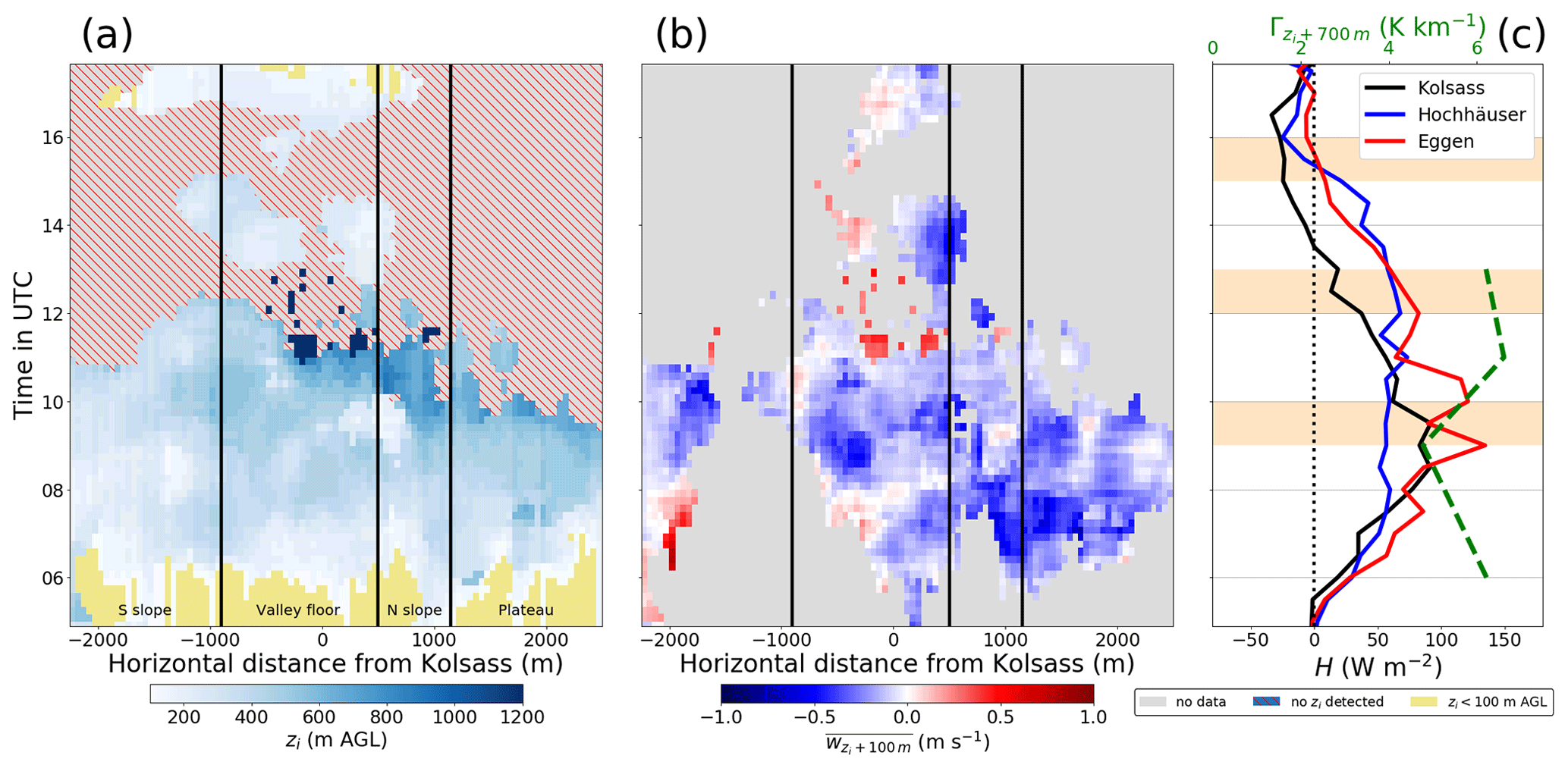
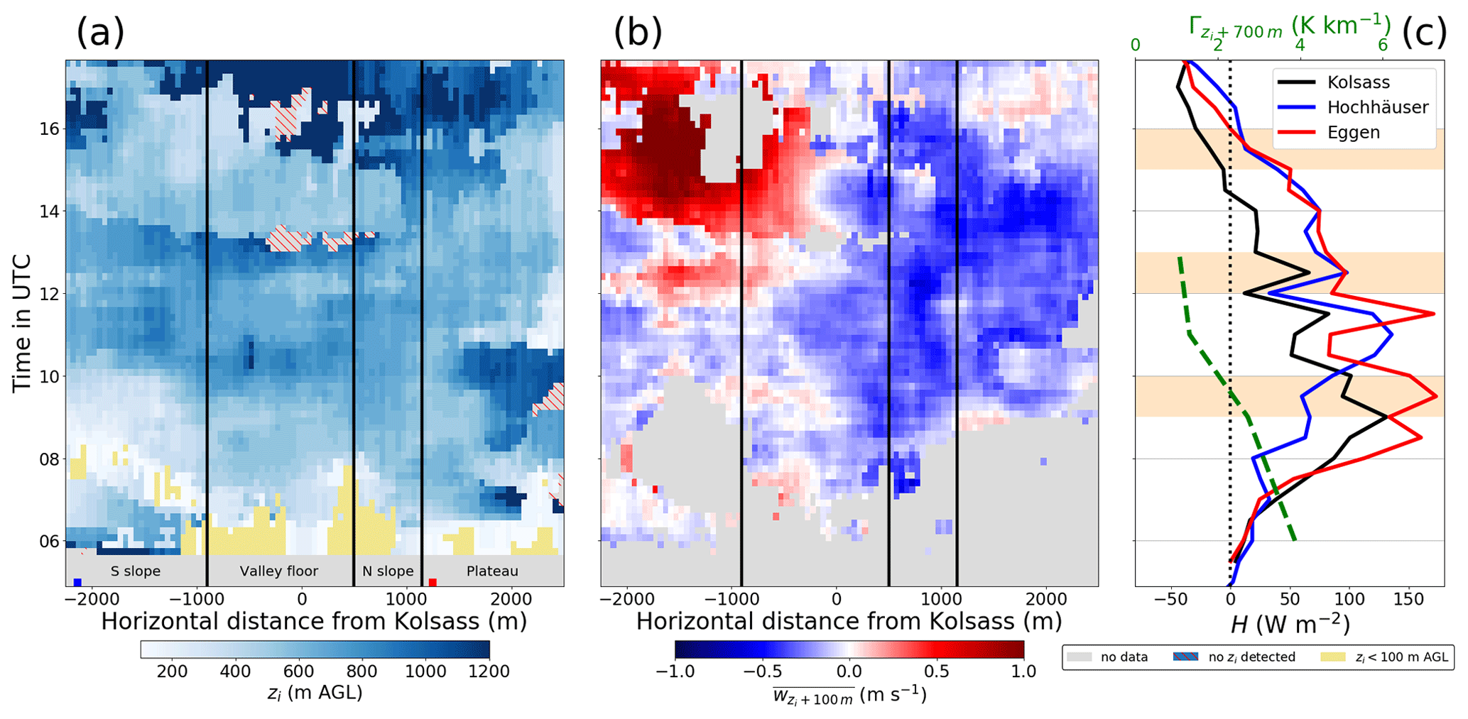
Concerning the behaviour of the other IOPs, the overall similarity between IOPs 2a and 4 is evident, i.e. somewhat higher z_i values over the valley floor and the southern slopes between 12:00 and 14:00 UTC (Figs. 8a, 11a). As already mentioned in Sect. 4.1, the deeper CBL on these two IOPs goes along with less resistance during their deepening, as their Γ values decreased in time from roughly 4 to 1 K km⁻¹ (Figs. 8c, 11c). The pronounced cross-valley asymmetry in the w field on IOPs 2a and 4 due to the CVV after 14:00 UTC, although similar, differs on IOP 4 owing to the relatively lower CBL still detectable by the bottom-up method. Furthermore, during the CVV phase (Fig. 11a), i.e. during the third regime (Fig. 7l), the deeper detected CVV over the plateau compared to the southern part of the valley is another significant difference compared to IOP 2a. Figure 9a indicates that IOP 2b had evidently the shallowest CBL of all four IOPs. This behaviour holds for the whole N–S cross-section, though z_i reached somewhat higher over the southern slope and plateau than over the valley floor until 14:00 UTC. As mentioned before, on this day a CVV did not develop in the afternoon (indicated by a nearly symmetric w field, Fig. 9b), while Γ was quite high in the morning (Fig. 9c). On IOP 3, despite the developing foehn, the CBL was nonetheless able to develop in a manner similar to the other IOPs until about 11:00 UTC (Fig. 10a). Afterwards, the continually descending foehn layer (Fig. 6g, k) reached the up to then undisturbed CBL, resulting in the inability of the bottom-up method to yield meaningful z_i anymore.

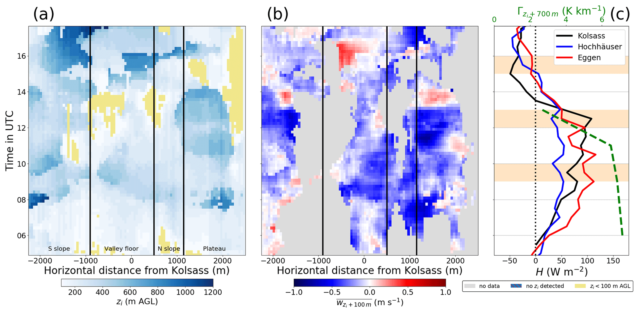
Figure 9 Same as in Fig. 8 but for IOP 2b. The short coloured bars indicating the locations of the respective i-Box sites have been omitted to avoid obscuring valid data.

Overall, being able to diagnose the CBL evolution in both time and space, based on measurements sampled solely by three lidars, a single radiosonde profile, and a handful of surface flux towers, provided us with information which would not have been attainable with profile measurements alone.

5 Discussion

Although we would have preferred to conduct year-round measurements to characterize the MoBL development throughout the annual cycle, we are confident that even a small number of days, e.g. a single week, may already yield valuable insight. Here we briefly address the applicability of the three identified MoBL regimes (Sect. 4.3) to other seasons. Based on the rest of the CROSSINN IOPs (Adler et al., 2021d; B21), as well as the well known climatology of yearly wind variability in the lower Inn Valley (Vergeiner and Dreiseitl, 1987), it is likely that shorter upvalley flow durations during wintertime prevent CVV formation, thus altering the late afternoon picture compared to our observations, specifically the third shear regime. Although wintertime H at the valley floor retains values comparable to summertime, LE decreases markedly comparing to summertime (Lehner et al., 2021, their Fig. S2), thereby enhancing the Bowen ratio and overall surface energy partitioning in favour of H, i.e. enhanced CBL growth. The spatial variability of both H and LE during wintertime is however more heterogeneous compared to summertime analysed in this study, which ultimately makes the MoBL in this region of the Inn Valley more prone to layering and asymmetric slope influences on the MoBL as a whole (Gohm et al., 2009). Foehn and cold pool occurrence and their interactions also become more frequent towards wintertime (Haid et al., 2020, 2022). The gradual foehn descent into the Inn Valley and eventual CBL erosion as on IOP 3 have already been documented in other valleys, for example on the island of Corsica during the HyMeX campaign (Adler and Kalthoff, 2016; Kalthoff et al., 2020). Additionally, several modelling studies have revealed the action of tributary valleys, such as the Wipp Valley, channelling the south foehn into the Inn Valley and deflecting eastward towards our investigation area (e.g. Gohm and Mayr, 2004, their Fig. 6a, b; Umek et al., 2021, their Fig. 6). Overall, depending on the season, we expect our three MoBL regimes to be present year-round, although with varying durations dependent primarily upon upvalley flow strength and synoptic perturbations.

Figure 10 Same as in Fig. 9 but for IOP 3.

Figure 11 Same as in Fig. 9 but for IOP 4.

The lower Inn Valley, with its approximate 20 km crest-to-crest width and depth of roughly 1500 m, has been used as a benchmark valley in multiple idealized numerical modelling studies of MoBL flows for more than a decade (Schmidli et al., 2011; Schmidli, 2013; Schmidli and Rotunno, 2015; Wagner et al., 2014, 2015; Lang et al., 2015; Leukauf et al., 2015, 2016, 2017; Weinkaemmerer et al., 2022, 2023). Our investigation area therefore fits closely into such a layout, thereby providing unique observational context for the above numerical experiments. Looking more globally, every valley exhibits some degree of along-valley curvature, sidewall asymmetry in terms of a plateau on one side, or presence of tributary valleys. As such, our study serves as an important observational evidence of the range of MoBL regimes expected to occur in a valley environment exhibiting all of the above. Although limited to the Alps, the results presented herein can nonetheless serve to help interpret potentially similar phenomena found to occur in non-Alpine valleys. More importantly, the novel method based on spectrum width detection of turbulent layers can find much broader usage beyond mountain meteorological applications. In other words, our study also served to demonstrate what types of analyses are feasible using the bottom-up method applied to highly spatially and temporally resolved spectrum width fields.

6 Conclusions

This study presented an investigation of the CBL and MoBL evolution in the CROSSINN investigation area, located to the east of the city of Innsbruck in the Inn Valley, Austria, over a single-week period during August 2019. Given the ongoing difficulty of adequately labelling any turbulent layer as either a CBL or a MoBL over complex terrain, we stuck with a more general labelling equal to CBL until the sign reversal of the surface sensible heat flux H from positive to negative, when we switched to denoting turbulent layers in general, irrespective of the turbulence origin, simply as constituting a turbulent boundary layer. By doing so, we opened up a more clear path towards a bigger emphasis on the evolution of the CBL, with the option of examining different MoBL developments once H changes its sign. During this week, four IOP events took place, specifically 2a, 2b, 3, and 4. A unique approach of studying the different CBL stages during the IOPs was possible due to turbulent Doppler spectrum width. Labelled as spectrum width in this study, it is a quantity carrying the signature of buoyantly and mechanically generated turbulence within the pulsed volume of a Leosphere WindCube WLS200s Doppler lidar. Three such lidars were deployed in a cross-valley transect, enabling not only the derivation of a true vertical and one horizontal wind speed component in the cross-valley plain with the coplanar retrieval method but also extending the areal coverage of spectrum width, up to 4 km horizontally and roughly 2 km vertically with a temporal resolution of 1 min.

By utilizing in situ aircraft and radiosonde measurements, we were able to develop a bottom-up threshold exceedance method which relies on the contrast of elevated spectrum widths within the CBL against lower levels found in the upper valley atmosphere and even the free troposphere. We have only been able to adequately estimate the CBL depth z_i when the surface sensible heat flux H was positive. To calibrate the method for convective circumstances, the optimal threshold was chosen based on a comparison against the z_i determined with the bulk Richardson number approach applied to virtual potential temperature θ_v from the radiosondes. Additionally, validation of spectrum width features in space against rapid in situ turbulence aircraft measurements further corroborated the promising capabilities of spectrum width for CBL evolution. Specifically, depending on the aircraft's vertical position with respect to local z_i, we found decent agreement between spatio-temporal average values of vertical velocity variances $\langle {w^{\prime }}^{\mathrm{2}}\rangle$ and kinematic heat and moisture fluxes $\langle w^{\prime }{\mathit{\theta }}^{\prime }\rangle$ and $\langle w^{\prime }{q}^{\prime }\rangle$ with theoretical expectations in cases whenever spectrum width was elevated. When spectrum width was generally lower, as is the case above the CBL, these quantities reflected different sign relationships and magnitudes, indicating either the entrainment zone or the free troposphere.

Through an examination of the temporal evolution of spectrum width above the valley floor, we established the primary spectrum width features at each developmental stage of the MoBL during the four IOPs. The deepest CBLs were found on IOPs 2a and 4, during which synoptic influence on the valley atmosphere was weakest. On the other hand, shallowest CBLs occurred on IOP 2b, which was primarily attributed to the strongest upper-level Γ and partly to foehn influence. Compared to HHF terrain, where CBL typically achieves depths up to 1500 m or more (Stull, 1988), the CBL in the investigation area was rarely deeper than 900 m. This is primarily due to strong static stability and much stronger subsidence above the CBL than that commonly found over HHF terrain. In afternoon hours, the presence of the CVV was expressed via spectrum widths much larger than those found earlier in the day within the CBL. Since the CVV is primarily a phenomenon characterized by pronounced shear in face of a negative H, the poorer performance of the bottom-up method reflected this state. The most unique aspect of this study was the cross-valley spatio-temporal evolution of both z_i and w_L in the form of a time–distance diagram, a visualization technique that has up to now been mainly possible using large-eddy simulations for these parameters. Overall, relying on a technique that depends on turbulence properties helped highlight the limited representativeness of point measurements in complex terrain. Even under clear sky conditions, the already heterogeneous character of the MoBL found in our cross-valley transect may become substantially more complex under synoptic influence. In such situations, traditional ABL depth detection methods become inadequate, invoking the need for methods which better reflect turbulence features, such as those found during CVV occurrence.

The main take-away of the present study is the introduction of three distinct regimes that characterize the state of the MoBL in the Inn Valley from sunrise to shortly after sunset. During the first regime the CBL may be expressed as a rapidly growing CBL but also as just a part of the overall MoBL. This growth is driven primarily by H, while its main opposing factor is Γ. The end of this regime is characterized by highest H achieved during the day, as well as a distinct terrain-following z_i across the valley, regardless of Γ or w_L magnitude. The second regime describes the period when H is decreasing simultaneously with an intensifying upvalley flow. Effects of Γ and w_L now become increasingly more influential, leading eventually to a case-dependent cross-valley pattern of z_i, ranging from horizontally level to still terrain-following. The sign change of H, accompanied with the strongest upvalley flow during the day, marks the onset of the third and final regime. If the appropriate conditions are met, namely a sufficiently potent upvalley flow and negligible synoptic influence, the turbulent boundary layer at this time and in this particular cross-section of the Inn Valley will primarily be characterized by the CVV, which typically dissipates entirely a few hours after sunset, marking the beginning of stable MoBL formation.

Although the bottom-up exceedance method aided us in untangling the subtleties of daytime MoBL evolution in the Inn Valley, it also raised several additional questions, the answers of which remain outside of the scope of the present work. For instance, the origin of upper-level turbulence regions prior to CVV generation or foehn arrival, particularly when viewing the entire transect (e.g. Figs. 3a, b and 7d, e), remains suspect. While we hypothesize such regions stem either from directional shear with height, they may also be advected pockets of turbulence generated upstream. The occurrence of a large spectrum width layer close to the surface, together with an intense upvalley flow jet present at the same time, highlights the potential benefit of using spectrum width in studying katabatic flows down valley sidewalls. In other words, properly executed RHI or plan position indicator (PPI) scans above such slopes may provide a unique insight into the variability of intermittent turbulence found underneath otherwise very shallow katabatic jets during stable, nighttime conditions. Despite advancing our understanding of the MoBL structure in the Inn Valley owing to a novel sampling technique, a number of unresolved questions remain. As for the along-valley representativity of our findings, tightly linked to along-valley MoBL heterogeneity, properly designed aircraft or UAS measurements could be utilized. However, given the high cost of flight hours, reliance on remote sensing approaches is superior in this regard. To gain a deeper insight into heterogeneity, we argue that the spectrum width methodology could be extended as well, by coupling multiple remote sensing lidar systems along the Inn Valley. Doing so would in turn enable estimates of the still elusive horizontal advection terms (Eq. 1), neglection of which is unjustified in complex terrain. On the other hand, although we have been able to provide highly resolved cross-valley transects of z_i and w_L, our conclusions were nonetheless restricted to having just three discrete sites offering H. To truly explore the CBL growth framework, similar highly resolved transects of H are necessary, a demand potentially fulfilled with an array of carefully sited scintillometers (Ward, 2017). We are confident that the upcoming Multi-scale Transport and Exchange Processes in the Atmosphere over Mountains (TEAMx) programme and experiment (Serafin et al., 2020; Rotach et al., 2022) will offer the necessary means and resources to address these remaining challenges.