the Creative Commons Attribution 4.0 License.
the Creative Commons Attribution 4.0 License.
 | 02 Jul 2024
Deepening mechanisms of cut-off lows in the Southern Hemisphere and the role of jet streams: insights from eddy kinetic energy analysis
Henri Rossi Pinheiro
Kevin Ivan Hodges
Manoel Alonso Gan
Cut-off lows (COLs) exhibit diverse structures and lifecycles, ranging from confined upper-tropospheric systems to deep, multi-level vortex structures. While COL climatologies are well documented, the mechanisms driving their deepening remain unclear. To bridge this gap, a novel track matching algorithm applied to ERA-Interim reanalysis investigates the vertical extent of Southern Hemisphere COLs. Composite analysis based on structure and eddy kinetic energy budget differentiates four COL categories: shallow, deep, weak, and strong, revealing similarities and disparities. Deep, strong COLs concentrate around Australia and the southwestern Pacific, peaking in autumn and spring, while shallow, weak COLs are more common in summer and closer to the Equator. Despite their differences, both contrasting types evolve energetically via anticyclonic Rossby wave breaking. The distinct roles of jet streams in affecting COL types are addressed: intense polar front jets correlate with more deep COLs, whereas stronger subtropical jets relate to fewer shallow COLs. The COL deepening typically occurs in the presence of a robust upstream polar front jet, which enhances ageostrophic flux convergence and baroclinic processes. The subtropical jet positively correlates with COL intensity but weakens when considering the seasonality, suggesting uncertainties in this relationship. Additionally, we highlight the significance of diabatic processes in COL deepening, addressing their misrepresentation in reanalysis and emphasizing the need for more observational and modelling studies to refine the energetic framework.
- Article
(5046 KB) - Full-text XML
-
Supplement
(1480 KB) - BibTeX
- EndNote


Cut-off low-pressure systems are closed low-pressure systems that detach or “cut off” from the main westerly flow (Palmén, 1949). These systems manifest as isolated cyclonic potential vorticity anomalies and form both equatorward and poleward of the polar front or mid-latitude jet (Portmann et al., 2021). Cut-off lows (COLs) are known for their slow movement, varying in duration from short-lived to persisting for several days. Their prolonged periods of precipitation often result in significant accumulations and eventually floods (Singleton and Reason, 2007; Llasat et al., 2007; McInnes and Hubbert, 2011).
One critical aspect of COLs is their vertical extent, which directly influences their precipitation intensity and duration. Deep COLs, reaching lower-atmospheric levels, are usually linked to heavier rainfall compared to shallow systems (Porcù et al., 2007; Pinheiro et al., 2021). Early studies (Palmén, 1949) have established the groundwork for understanding their vertical structure, revealing their key features, such as a quasi-barotropic structure, tropopause folding, and thermal dipole patterns. Subsequent studies, including those of Frank (1970) and Porcù et al. (2007), have observed a clear relationship between COL vertical extent and the associated cloud and precipitation patterns. More recently, Portmann et al. (2021) highlighted the influence of jet streams on the precipitation intensity of COLs based on their relative position.
Significant progress has been made in understanding the mechanisms driving the development of COLs. Studies have shed light on the crucial role of jet streams in supplying energy to these systems (Pinto and da Rocha, 2011; Gan and Dal Piva, 2013; Ndarana et al., 2021). Their formation often results from a split flow associated with Rossby wave breaking, leading to convergence of ageostrophic geopotential fluxes (hereafter, ageostrophic fluxes) and baroclinic processes (Ndarana et al., 2021; Pinheiro et al., 2022). Diabatic processes, such as radiative cooling and latent heating, also play a role in COL development (Sakamoto and Takahashi, 2005; Garreaud and Fuenzalida, 2007; Cavallo and Hakim, 2010; Portmann et al., 2018).
Despite these advancements, a comprehensive understanding of COL deepening mechanisms remains unclear. The role of jet streams in deepening COLs and the complex influence of diabatic processes require further investigation. Elucidating these key aspects is crucial for both accurate predictions and improved understanding of COL dynamics. This study aims to address these critical gaps by addressing the following scientific questions:
-
How sensitive are methods for estimating the vertical depth of COLs?
-
Can COLs be affectively classified based on their intensity and vertical depth? Do these classifications differ in terms of their spatial distribution and temporal variability?
-
How do jet streams influence COLs? Does the influence on deepening mechanisms differ between different COL types? Can specific jet stream characteristics be identified as particularly conducive to the deepening of COLs?
By addressing these key questions, we hope to significantly improve our understanding of COLs and their role in atmospheric dynamics. The remainder of the paper is organized as follows. Section 2 outlines the data and methods employed for tracking, estimating vertical depth, and producing composites of the structure and energetics of COLs. Section 3 presents the results, and finally, Sect. 4 provides a summary of the main findings and conclusions.
2.1 Reanalysis dataset and tracking methodology
This study uses the ERA-Interim reanalysis data (Dee et al., 2011) obtained from the European Centre for Medium-Range Weather Forecasts (ECMWF) for the period from 1979 to 2014. ERA-Interim reanalysis employs a spectral model with an N128 reduced Gaussian grid (∼ 80 km) and 60 vertical hybrid levels, produced with a four-dimensional variational data assimilation (4D-Var) system.
Before the tracking, the data are spectrally truncated at 42 wavenumbers (T42), and coefficients corresponding to total wavenumbers less than five are set to zero. This is done to reduce noise and eliminate large-scale background influences, similarly to previous work (Pinheiro et al., 2017, 2021, 2022). The established TRACK algorithm (Hodges, 1995, 1996, 1999) is employed to track T42 vorticity minima at various pressure levels (1000, 900, 800, 700, 600, 500, 400, and 300 hPa), using a consistent threshold (−1.0 × 10⁻⁵ s−1) intentionally set relatively low to capture diverse cyclonic systems. The tracking is performed by minimizing a cost function for track smoothness subject to adaptive constraints on track smoothness and displacement distance. The tracking algorithm is the same as the one used for extratropical and tropical cyclones (e.g. Hodges et al., 2011, 2017) but with some adjustments to the slower movement of COLs, as discussed in Pinheiro et al. (2019). The resulting tracks are filtered based on horizontal wind components (u,v) at four 5° geodesic offset points from the vorticity centre: 0° (u>0), 90° (v<0), 180° (u<0), and 270° (v>0) relative to the north. This retains only closed cyclonic centres, as discussed in Pinheiro et al. (2019). The retained tracks are those that either move equatorward and reach latitudes north of 40° S or originate north of 40° S and persist for at least 24 h.
Spatial statistics of the COLs are computed using the track information and spherical kernel estimators for track density and mean intensity (Hodges, 1996). Track density represents COLs per season per unit area (5° spherical cap ≅ 106 km2), while mean intensity derives from T42 relative vorticity, scaled by −1 for the Southern Hemisphere.
2.2 Approach to estimate the vertical depth of COLs
To analyse and quantify COLs, numerous algorithms have emerged, though only a few of them address multi-level cyclone detection and their connections. Existing algorithms establish cyclone position correspondence between levels based on feature point distances, utilizing geopotential or vorticity centres. These methods span from basic search tasks (Lim and Simmonds, 2007; Porcù et al., 2007) to more advanced techniques based on optimal solution (Lakkis et al., 2019).
In this study, the track matching algorithm introduced by Hodges et al. (2003) and used to match tracks in different datasets (Bengtsson et al., 2009; Hodges et at., 2011, 2017; Pinheiro et al., 2020) is employed to match tracks between different pressure levels. The algorithm is used to compare tracks across different pressure levels by defining a mean separation distance (dm), chosen here to be 5° geodesic, and considering overlaps in time (χ) between corresponding points in the tracks. Temporal overlaps between tracks are determined following a sensitivity analysis, as discussed in Sect. 3.1. The percentage of points overlapping in time is calculated using the approach described in Hodges et al. (2003), defined as follows:
where nm is the number of points that match in time, and n1 and n2 are the number of points in the track corresponding to different pressure levels.
Since our focus is on the upper-level forcing driving surface cyclone development and the mechanisms governing this interaction, our method works in a top-down manner, starting with two levels at a time and progressively extending the matches to adjacent pressure levels. Vorticity tracks (ξ300) are matched against ξ400 if the mean separation distance is ≤ 5° and temporal overlap exists. Successful matches indicate extending COLs; unmatched ξ300 tracks imply the COL is confined to 300 hPa. An iterative process continues to lower levels (500, 600 hPa, and so on), stopping at the last match at 1000 hPa. The deepest successful match determines the COL vertical extent.
Complex interactions between COLs and lower-level cyclonic features make capturing the full range of coupling processes challenging. Our algorithm, while simpler than the optimal solution-based approach in Lakkis et al. (2019), consistently establishes vertical associations and a sequential stacking process. However, diverse matching procedures might result in distinct COL evolution outcomes, although prior research has shown similar results between bottom-to-top and top-to-bottom approaches (Lakkis et al., 2019).
2.3 Compositing analysis of the structure and energetics of COLs
Employing a system-centred compositing method similar to that of Pinheiro et al. (2022), we investigate the composite structure of COLs and their eddy kinetic energy (EKE) budget. Initially, COLs are identified and categorized into shallow, medium, and deep types based on their vertical extent; however, due to space constraints only the findings concerning deep and shallow COLs are presented in the paper. Shallow COLs are limited to the upper troposphere, extending no lower than 400 hPa, while deep COLs originate at high levels and extend down to 800 hPa or lower. The depth levels are chosen to capture the contrasting vertical extents of COLs, which are typically found in either the upper or the lower troposphere. These depth categories, each accounting for around 30 % of the total COLs, are chosen to ensure a balanced representation across different types in our analysis. Additionally, we classify COLs as strong (above the 50th percentile) or weak (below the 50th percentile) according to their maximum intensity observed along each track, based on the 300 hPa vorticity.
Atmospheric fields and energetic quantities are sampled on a 25° latitude–longitude rectangular grid, initially defined centred on the Equator then rotated to the COL 300 hPa vorticity centre, with a horizontal resolution of 0.5°. The sampling is performed at each vertical level from 1000 to 100 hPa, taking the 300 hPa track point as the reference. We present vertical composites for west–east cross-sections centred on the vorticity centre. These composites are produced for various time intervals relative to the peak intensity of COLs, but only times within ±48 h of the peak intensity are shown. Extending the compositing window beyond this time frame often introduces noise due to variations in COL lifetimes.
Using the Orlanski and Katzfey (1991) method, we investigate the energy dynamics associated with the COL deepening through the EKE budget. This approach considers essential mechanisms such as baroclinic and barotropic conversions and ageostrophic flux convergence (downstream development). In this study, the focus is on baroclinic conversion and ageostrophic flux convergence, the two primary EKE budget mechanisms in COLs (Gan and Dal Piva, 2016; Ndarana et al., 2021; Pinheiro et al., 2022).
The budget residual accounts for processes not fully captured by the EKE budget calculation, including friction and discretization errors such as interpolation and finite differences. Errors could also arise from how diabatic processes are represented in reanalysis products (Pinheiro et al., 2022). Time-mean quantities are calculated for each month averaged over 28–31 d for the 6-hourly data, separately for each individual month and year.
2.4 Link with jet streams
The connection between COL extent and jet streams is also explored using Pearson correlation coefficients and scatterplots. Following Bals-Elsholz et al. (2001), the characteristics of the polar front and subtropical jets are defined by averaging the 300 hPa zonal mean zonal wind at 50–65° S and 25–35° S, respectively. The polar front jet, characterized by large zonal variations, is defined as a wide latitudinal band, contrasting with the subtropical jet, which exhibits relatively minor spatial and seasonal variations in its position within the Southern Hemisphere (Simmonds and Jones, 1998). Correlation coefficients are employed to verify the relationship between jet strengths and COLs, with significance exceeding 95 % and 99 %.
3.1 Sensitivity of track matching algorithm for the estimation of COL depth
To assess the sensitivity of the track matching algorithm in determining COL depth, we investigate the influence of the mean separation distance (dm) and temporal overlap (χ) between tracks at different pressure levels. We systematically varied χ from 1 % to 100 % while keeping dm fixed at 5° geodesic. This choice is based on observations that the depth estimation is more sensitive to χ than dm. Setting dm to a large value leads to a significant rise in the number of matches; however, this can introduce false matches involving unrelated cyclonic systems. Therefore, we set dm to 5° geodesic, which is suitable considering the typical small vertical tilt of COLs (refer to Fig. 9 in Pinheiro et al., 2021).
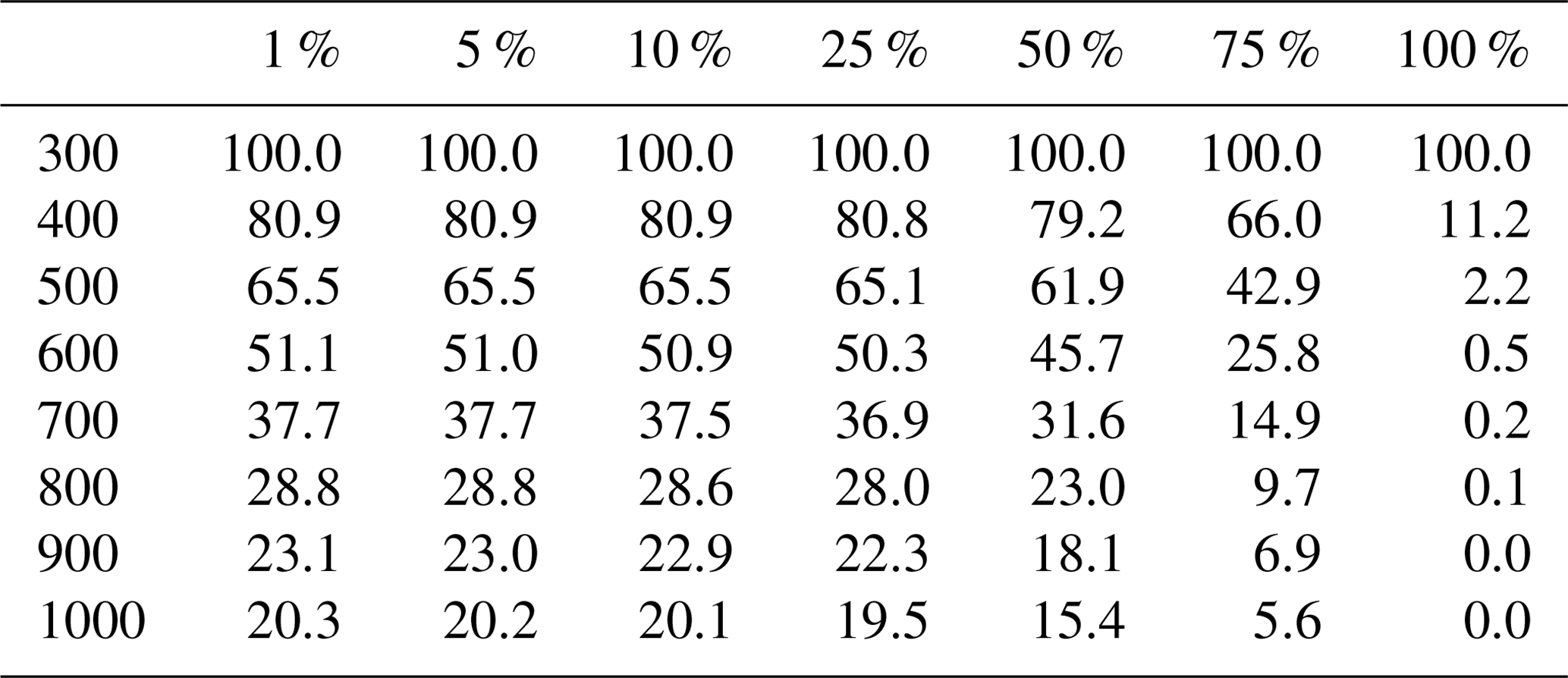
A sensitivity analysis varied χ across a range of values. Setting χ to 1 % requires a minimum of 1 % time overlap between tracks at different pressure levels. Table A1 in the Appendix shows that 20.3 % of ξ300 COLs extend to the surface in at least one time step, indicating interconnected cyclonic features across all levels from 300 to 1000 hPa. The number of systems reaching the surface remains relatively consistent for χ values ranging from 1 % to 25 % at 20.3 % to 19.5 % of all COLs. However, matches significantly decrease when χ exceeds 50 %, likely due to COLs only associating briefly with lower-level features. With χ set to 75 %, less than 10 % of systems are identified as deep COLs, suggesting an underestimation due to association with short-lived lower-level features. Relaxing the χ threshold increases the chance of capturing a stacked cyclonic system, guaranteeing vertically aligned or tilted COLs across adjacent levels using χ= 1 % and dm= 5°.
Using geopotential data instead of relative vorticity to estimate COL depth is an alternative approach. However, some care is required in selecting an appropriate threshold as geopotential magnitude generally increases with height in baroclinic systems. Previous studies (Porcù et al., 2007; Barnes et al., 2021) have used varying geopotential thresholds for each pressure level, requiring different subjective thresholds at each level. In contrast, vorticity-based identification does not require vertical adjustments, as vorticity measures atmospheric flow rotation. Moreover, weaker COLs are less likely to be identified in a geopotential field-based tracking method (Pinheiro et al., 2019).
3.2 Relationship between intensity and vertical depth of COLs
Classifying COLs by grouping similar systems is crucial for uncovering the key factors influencing their diverse types, allowing for a deeper understanding of their dynamics and providing a framework for evaluating climate impacts. This section explores the contrasting characteristics among four COL categories: shallow, deep, weak, and strong COLs (Fig. 1). These categories are defined based on intensity and vertical extent, as detailed in Sect. 2.3. While intermediate-level COLs exist, this study focuses on the contrasting features of their vertical extent. This analysis does not focus on vertical tilt, which is comprehensively addressed in Pinheiro et al. (2021).
Figure 1 shows the annual track density of COLs in the four categories described above. Deep and strong systems exhibit similar distribution patterns, both primarily concentrated in Australia and the southwestern Pacific, with a secondary maximum in the southeastern Pacific off the west coast of South America. These two groups exhibit similar intensity patterns, with maxima (blue dots) located in Australia and upstream of the main continents, as previously demonstrated (Barnes et al., 2021; Pinheiro et al., 2021, 2022). Shallow and weak COLs also share similarities; they are less intense and more dispersed than the deep and strong systems. These systems are predominantly found in the South Atlantic, southeastern Africa (Madagascar), and the southern Indian Ocean, and they are more frequently found equatorward than their deep and strong counterparts, a notable feature over the central-eastern Pacific Ocean.
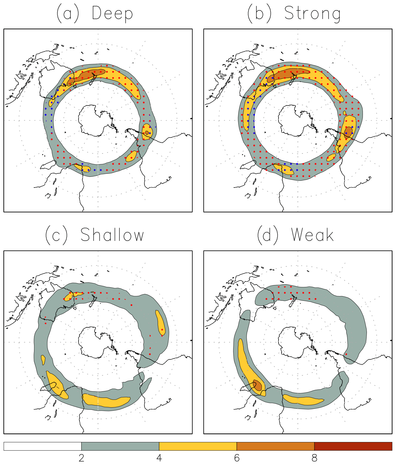
Figure 1Track density (shaded) and mean intensity (dots) for (a) deep, (b) strong, (c) shallow, and (d) weak COLs in the Southern Hemisphere. Track density is measured in number per season per unit area, where the unit area is equivalent to a 5° spherical cap (≅ 106 km2). Mean intensities less than −8 × 10⁻⁵ s−1 (−12 × 10−5 s−1) are represented with red (blue) dots.
By contrasting the tracks within each category, we found that 81 % of deep COLs correspond with the 50th percentile of the strongest systems, suggesting a significant correlation between the two categories. However, it is noteworthy that 19 % of deep COLs fall into the category of weak COLs, indicating a level of variance within this classification. Similarly, 71 % of weak COLs correspond to shallow COLs. Despite the similarities shared between strong and deep COLs, as well as weak and shallow COLs, it is important to recognize that they are not entirely comparable. These distinctions arise from differences in classification and the dynamics inherent in these systems and their development processes.
Figure 2 shows the seasonal variations in the average monthly number, intensity, and latitude of COLs for each of the four distinct categories. A clear correspondence in seasonality is evident between deep and strong COLs, as well as between shallow and weak types. Deep and strong COLs exhibit similar intensities (Fig. 2c), though the deepest systems display a more pronounced seasonal cycle in intensity compared to the strongest ones. Deep and strong COLs are more prevalent at 31–33° S (Fig. 2b) from autumn to spring, with two peaks in May and October (Fig. 2a). These peaks appear to be associated with a semiannual oscillation in the polar front jet, albeit with a 2-month delay after the first peak (Fig. 2d). The half-yearly cycle in the eddy-driven jet is attributed to a response of meridional temperature and pressure gradients between middle and high latitudes, which peaks during equinoctial seasons (Van Loon, 1967). Our findings align with previous studies and demonstrate a similar cycle to that observed for mid-latitude COLs and Rossby wave breaking events on the 330 K isentropic surface (Ndarana and Waugh, 2010; Favre et al., 2012).
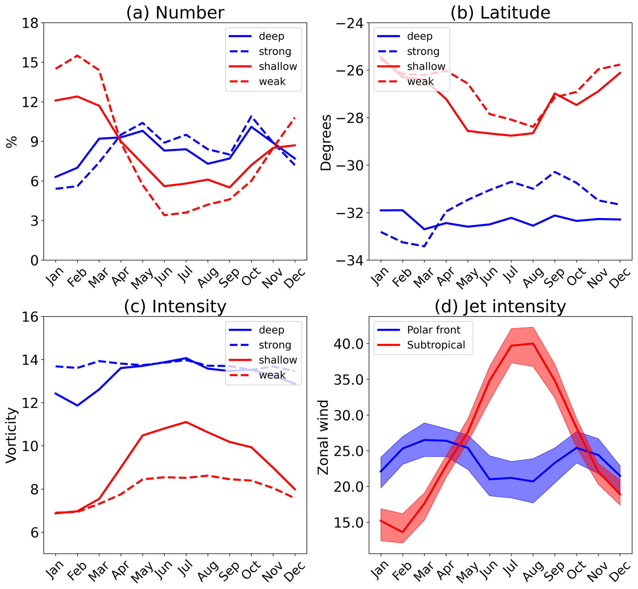
Figure 2Zonal monthly mean characteristics of COLs categorized by deep, strong, shallow, and weak for (a) number, (b) latitude reached at the time of maximum intensity, and (c) maximum intensity at 300 hPa vorticity (scaled by −1 × 10⁻⁵ s−1). (d) Intensity of subtropical and polar front jets as represented by the climatological 300 hPa zonal mean zonal wind at 25–35° S and 50–65° S, respectively.
In summer, shallow and weak COLs exhibit notably higher frequencies compared to the fewer occurrences observed in winter months. This seasonal pattern appears to be closely linked to the fluctuations in subtropical jet intensity, which experiences a decline (increase) in summer (winter). The increased (reduced) frequency of COLs appears to correspond with the weakened (intensified) subtropical jet strength in summer (winter). This association likely arises because shallow and weak COLs tend to occur more equatorward, roughly coinciding with the subtropical jet position (see Fig. 3). This aligns with the idea that COLs are primarily found over regions of weakened westerly winds (Nieto et al., 1998), and this hypothesis is supported by a robust negative correlation of −0.95 (−0.97) significant at 95 % between shallow (weak) COLs and subtropical jet intensity.
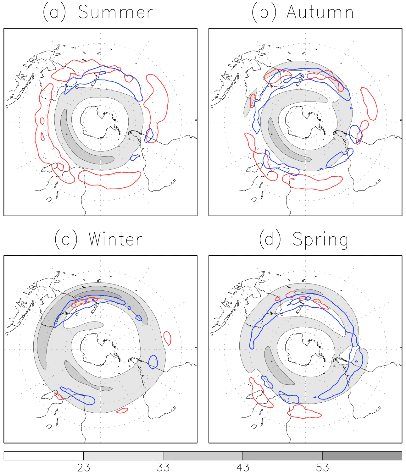
Figure 3Zonal mean wind (shaded) and track density for deep COLs (blue contour) and shallow COLs (red contour) in the Southern Hemisphere for (a) summer (DJF), (b) autumn (MAM), (c) winter (JJA), and (d) spring (SON). Unit is as in Fig. 1 for track density and in metres per second for zonal wind. Track densities are plotted for interval contours of four units. All fields are represented at the 300 hPa level.
Overall, there exists a discernible relationship between upper-tropospheric intensity of COLs and their vertical depth, establishing both classifications as pertinent parameters for assessing the vertical structure of these phenomena. The association of deeper COLs with stronger cyclonic vorticity can be attributed to geostrophic balance and the vertical coupling of atmospheric motions. Enhanced upper-tropospheric circulations induce increased vertical motions and static stability anomalies, resulting in the formation of deeper vertical structures. To maintain consistency and simplicity in our analysis, our subsequent investigations will solely concentrate on the classification based on COL depth.
3.3 Seasonal variations in jet–COL interactions
The interplay between COLs, jet streams, and Rossby wave breaking has been documented in previous studies (Ndarana and Waugh, 2010; Barnes et al., 2021). To unravel this relationship further and elucidate how jets influence COL deepening, we present seasonal mean maps of upper-level zonal winds and track density for deep and shallow COLs, as illustrated in Fig. 3. A distinct polar front jet, often referred to as the mid-latitude jet in the literature, is apparent from the South Atlantic to the South Pacific oceans throughout the year, exhibiting a poleward spiraling pattern. In the Australia–New Zealand sector, the well-known split jet flow becomes more pronounced during the cool season due to a stronger subtropical jet (Fig. 3c). This pattern results in weak westerlies between the jets, inducing anticyclonic vorticity on the equatorward side of the subtropical jet and cyclonic vorticity poleward (refer to Fig. S2).
Deep COLs occur at more poleward latitudes and typically near the equatorward exit region of the polar front jet. This is particularly noticeable around Australia, albeit with some seasonal and spatial variations. During winter, COLs are less frequent but more intense than in other seasons (see Fig. 2), which might be a result of a stronger subtropical jet, which generates a cyclonic vorticity anomaly over its poleward side. Conversely, the subtropical jet is weak or absent in summer, when a higher occurrence of shallow, weak COLs is observed, particularly over the oceans and closer to the Equator compared to deep systems. Interestingly, deep COLs peak in autumn and spring, coinciding with a strengthened polar front jet reaching a comparable magnitude to the subtropical jet. Additionally, during transitional seasons, a secondary maximum in deep COLs is observed near the west coast of South America, particularly in spring when the maximum density occurs with reduced zonal flow at the end of the polar front jet on the poleward side of the subtropical jet.
Our findings support the idea that the subtropical and polar front jets affect COLs differently, aligning with previous observations of their contrasting effects on Rossby wave breaking and COL development (Ndarana and Waugh, 2010; Muñoz et al., 2020). While the polar front jet seems to favour the COL deepening, the subtropical jet emerges as a key mechanism for their intensification. However, uncertainty persists regarding the exact relationship between subtropical jet intensity and COL intensity. It is notable that while Rossby wave breaking and COLs manifest over reduced zonal flow which generally occurs in regions of weak climatological zonal winds, the mechanisms conducive for COL deepening and/or intensification are more likely in the proximity of jets. This is supported by earlier observations indicating that a stronger polar front jet leads to a more pronounced dipole pattern with enhanced cyclonic and anticyclonic vorticity anomalies (Bals-Elsholz et al., 2001). A more detailed discussion on the influence of jet streams in COLs is provided in the following sections.
3.4 Distinct effects of polar front and subtropical jets on COL depths
To further investigate the influence of jets on COLs, scatterplots are employed to visualize the relationship across different jet intensities, as given in Fig. 4. Following the approach detailed in Sect. 2.4, we found a moderate positive correlation between COL number and polar front jet intensity (r=0.47 at 99 % confidence level), implying that intensifying polar front jets are correlated with an increased occurrence of deep COLs. This correlation accounts for approximately 22 % of the variability in deep COLs. Shallow COLs also show a positive correlation with the polar front jet intensity but weaker than that for deep COLs (r= 0.25, p<0.01), explaining only 6 % of their variability. Considering the subtropical jet (Fig. 4b), no significant relationship with the occurrence of deep COLs is observed. In contrast, a significant negative correlation of 0.75 (99 % confidence level) is found for the relationship between the intensified subtropical jet and the reduction in shallow COLs. Approximately 56 % of the variability in shallow COLs can be attributed to changes in subtropical jet intensity, aligning with their seasonal variations, as illustrated in Fig. 2.
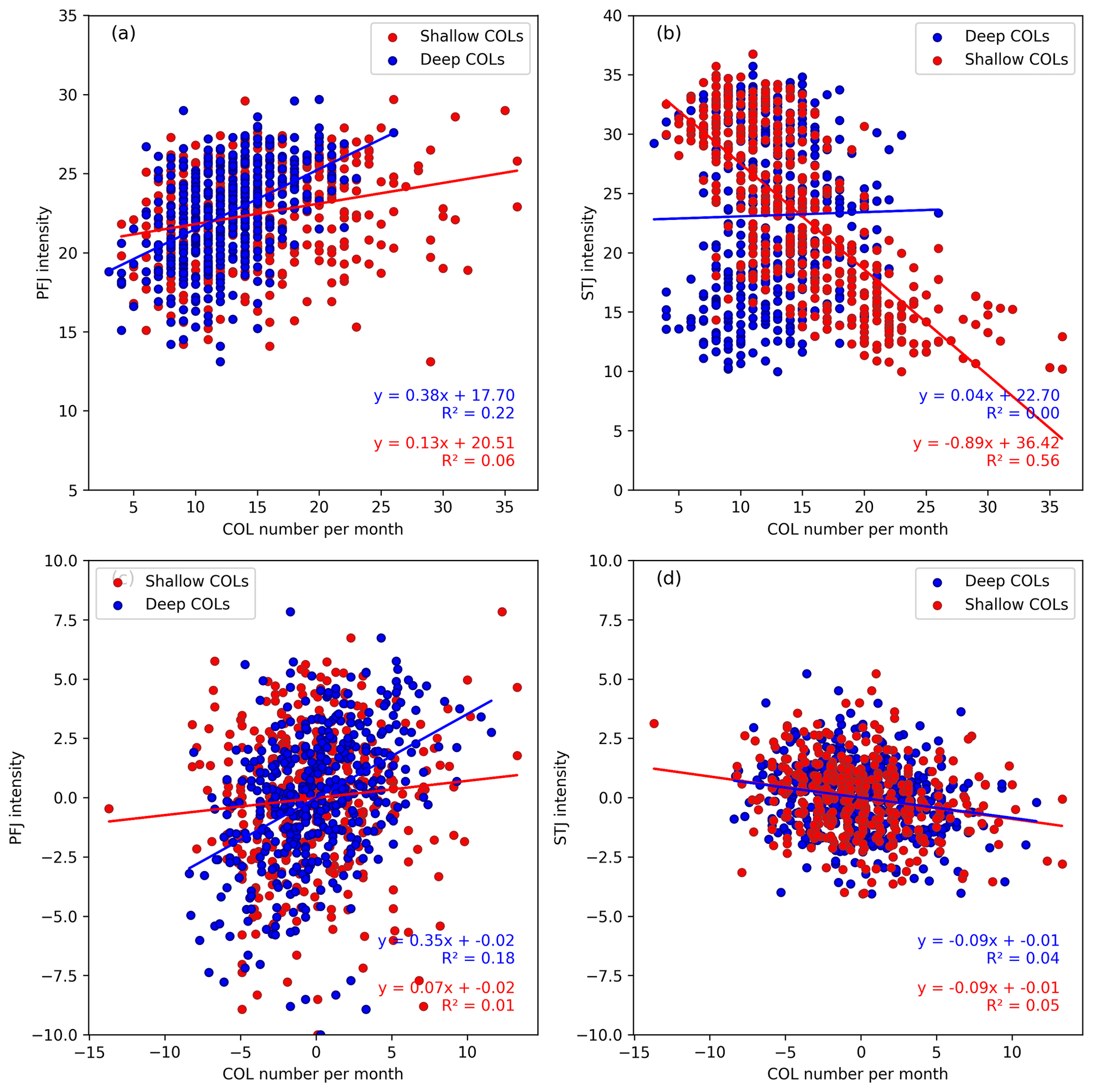
Figure 4Scatterplots indicating the relationships between the monthly mean COL number and jet intensity for (a, c) polar front jets and (b, d) subtropical jets using (a, b) raw values and (c, d) anomaly values. Anomalies are calculated by subtracting the monthly climatological mean from the observed value. Deep and shallow COLs are depicted by the blue and red colours, respectively. Unit is in m s−1 for jet intensity.
However, whilst the raw counts show a robust relationship between the intensified subtropical jet and the reduction in shallow COLs (see Fig. 4b), the strength of this relationship weakens when the seasonal cycle is removed from both variables (Fig. 4d). This is also observed for the relationship between the polar front jet and deep COLs (Fig. 4c). Hence, whilst there are issues in removing the seasonal cycle as a fixed factor (Pezzulli et al., 2005), the relationship between the strength of the subtropical and polar front jets and COLs remains a hypothesis due to its uncertainty, which requires further study.
Our analysis reveals a notable positive correlation between the intensity of both shallow and deep COLs and the subtropical jet (refer to Fig. S3), but the strength of these relationships weakens when the seasonal cycle is removed. This weakening is likely due to the pronounced seasonal cycle in the subtropical jet compared to the monthly variations from climatological means (as shown in Fig. S4). Removing the seasonal cycle weakens the signal, posing a limitation in considering the annual cycle as a fixed factor (Pezzulli et al., 2005). This highlights some uncertainty regarding these relationships, suggesting the need for further work to understand the influence of the jets and their seasonal cycle on the COL intensity. Additionally, no significant relationship is found between the intensity of COLs and the polar front jet (Fig. 4c), implying that the polar front jet primarily influences the variability of COLs rather than their intensity.
These differential effects likely arise from the distinct positions and roles of both polar front and subtropical jets within the large-scale atmospheric circulation. The polar front jet, primarily occurring at middle and high latitudes, is an eddy-driven jet associated with enhanced temperature gradients and baroclinicity. In contrast, the subtropical jet, situated around 25–30° S, arises from the momentum flux of the meridional circulation at the Hadley cell edge, which seems to act as a waveguide for Rossby wave breaking associated with 200 hPa COLs typically found at lower latitudes (Muñoz et al., 2020). The results of this study corroborate previous findings regarding the formation of COLs under reduced zonal wind. However, it is important to emphasize that the presence of a nearby jet is crucial for providing the energy necessary for the intensification and/or deepening of the system. A more detailed discussion on the jet–COL interaction is provided in the next section.
3.5 Shallow COLs vs deep COLs: contrasting from an energetics point of view
When it comes to unravelling the intricate mechanisms behind the deepening of COLs, understanding the role of specific mechanisms in determining their vertical extent can be aided by examining their energetics. Early studies have investigated the dynamical mechanisms of COLs by examining their vertically integrated energy budgets (Gan and Dal Piva, 2013, 2016; Ndarana et al., 2020; Pinheiro et al., 2022). In this study, we adopt a similar approach but direct our attention towards the two primary contributing mechanisms of the EKE budget: baroclinic conversion and ageostrophic flux convergence. We compare deep and shallow COLs and investigate the possible implications of energetics for their deepening.
Figures 5 and 6 show the temporal evolution of composite shallow and deep COLs, respectively, for horizontal and vertical fields. The four stages described in the conceptual model of Nieto et al. (2005) and shown in Pinheiro et al. (2021) are seen to be reproduced for shallow and deep COLs, involving the following stages: upper-level trough (−48 h), tear off (−24 h), cut off (0), and decay or dissipation (+24 and +48 h). Time is referenced to the time of maximum intensity in the 300 hPa vorticity.
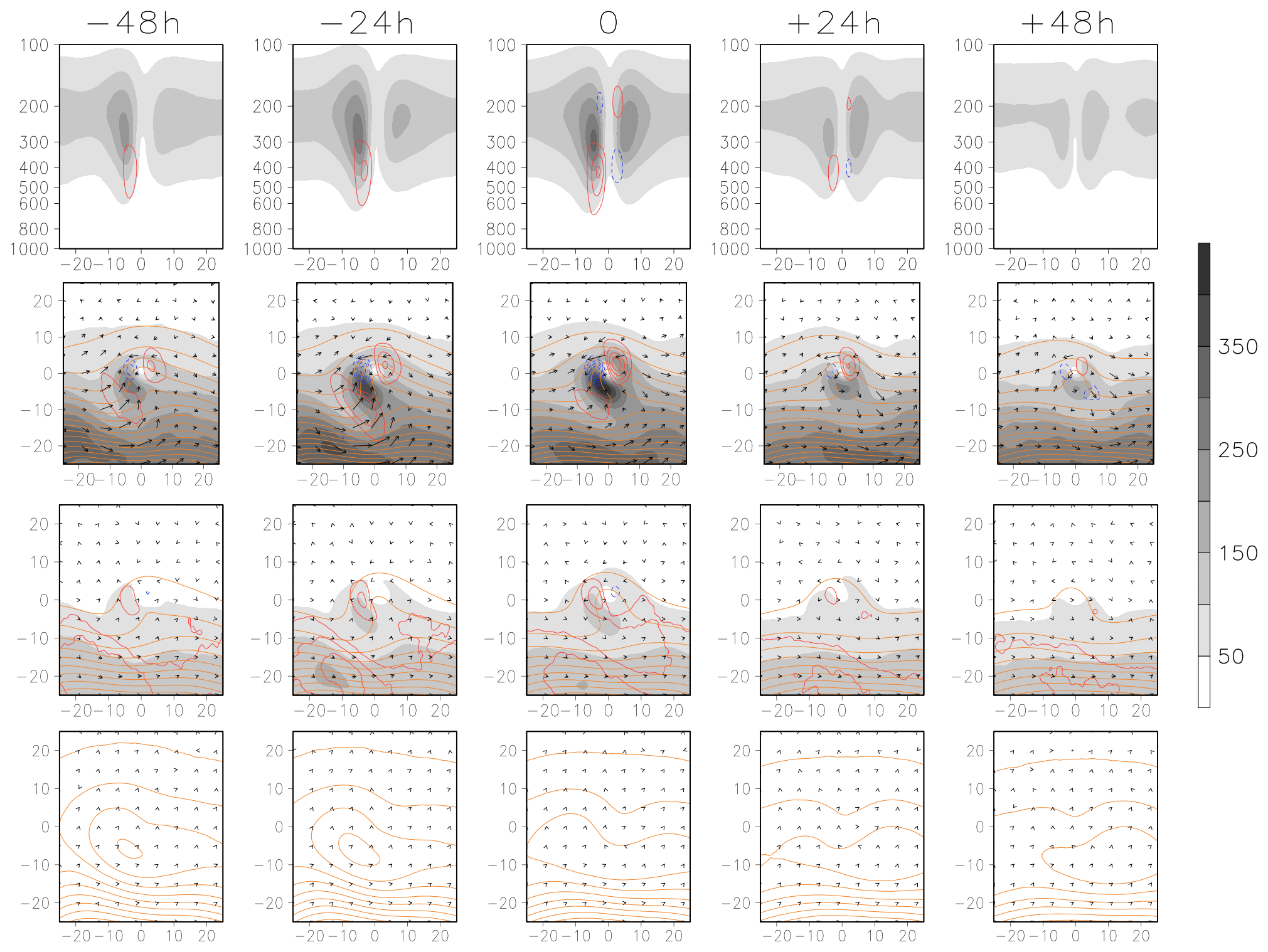
Figure 5Temporal evolution of shallow COLs in the Southern Hemisphere relative to the time and space of maximum intensity in ξ300. The panels depict the following: (a) vertical cross-sections of total EKE (shaded) with baroclinic conversion (contour); (b) vertically integrated ageostrophic flux convergence (contour) with EKE (shaded), geopotential height (orange line), and ageostrophic fluxes (vectors) at 300 hPa; (c) vertically integrated baroclinic conversion (red contour) with EKE (shaded), geopotential height (orange line), and ageostrophic fluxes (vectors) at 500 hPa; and (d) EKE, geopotential height (orange line), and ageostrophic fluxes (vectors) at 1000 hPa. Contours represent 0.003 × 10¹⁰ J s−1 for integrated quantities, 50 gpm for geopotential height at 300 and 500 hPa, and 20 gpm for geopotential height at 1000 hPa, while total EKE is indicated by 109 J.
In the upper-level trough and tear-off stages of shallow COLs (T= −48 h and T= −24 h in Fig. 5), a poleward jet located upstream of the ridge axis, i.e. west of the COL, acts as the primary energy source for the COLs. Concurrently, ageostrophic fluxes transport EKE northeastward from the poleward jet to the rear side of the COLs, forming an energy centre downstream of the ridge axis, referred to as the western energy centre. As the trough–ridge system deepens in an anticyclonic orientation, the western energy centre expands due to the convergence of ageostrophic fluxes and positive baroclinic conversion that arises downstream of the ridge axis, driven by descending cold air (not shown). The eastward propagation of the poleward jet and its increasing zonal flow give rise to anticyclonic barotropic shear flow and subsequent potential vorticity overturning, as documented in prior studies (Ndarana et al., 2021; Pinheiro et al., 2022). The COL decay occurs when the poleward jet shifts to the east, ceasing to provide energy to the system, as shown in Fig. S5.
Differences in the structure and lifecycle of shallow and deep COLs are observed. While shallow systems exhibit a gradual weakening and anticyclonic circulation at the surface, deep COLs display a multi-level interconnected vortex structure, as illustrated in Fig. 6. During their development phase, deep COL systems exhibit stronger ageostrophic fluxes along the ridge axis and larger baroclinic conversion on the upstream poleward jet compared to shallow systems. The positioning of deep COLs near the equatorward exit region of a strong polar front jet (as depicted in Fig. 3) intensifies the convergence of ageostrophic fluxes, thereby increasing baroclinic conversion. Consequently, this amplification leads to heightened vertical motions and deeper circulation. This distinct feature is prominently observed within deep COLs, distinguishing them from their shallow counterparts.
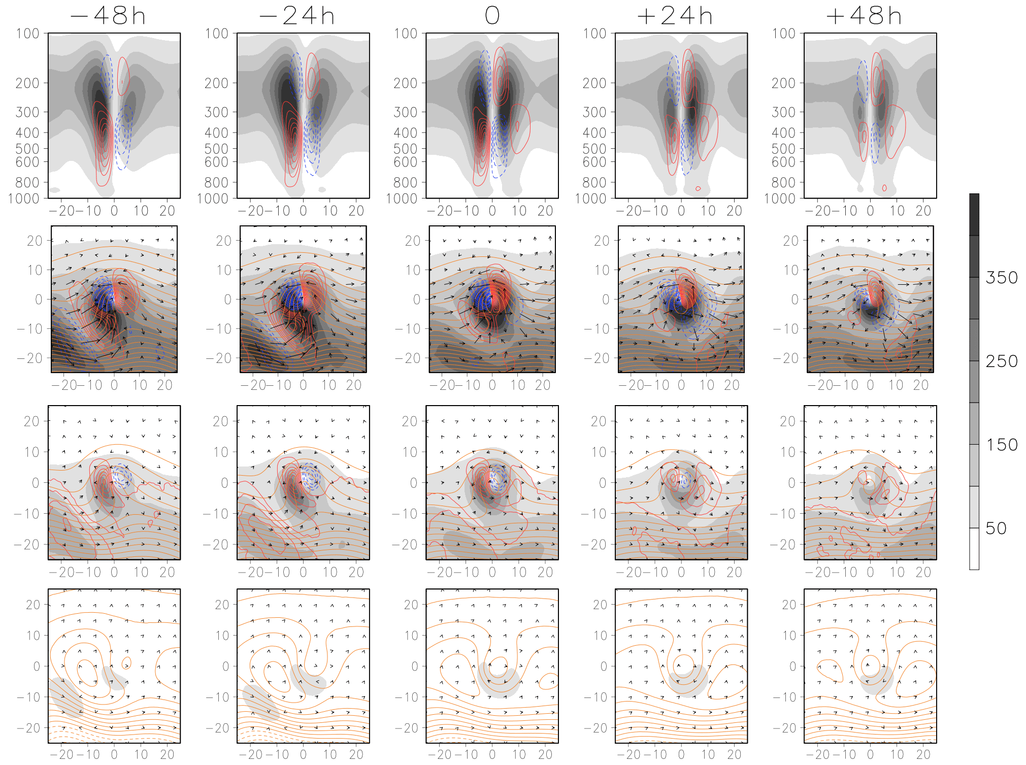
Figure 6The same as Fig. 5 but for deep COLs in the Southern Hemisphere. The dashed lines at the bottom indicate negative geopotential height at 1000 hPa.
Another distinct aspect of deep COLs arises during the cut-off stage (T= 0 onward), when enhanced vertical motions drive increased baroclinic conversion towards the east and near the surface. The interaction between upper- and lower-tropospheric eddies, as in mid-latitude baroclinic waves (Hoskins and Karoly, 1981; Trenberth, 1991; Nakamura, 1992), suggests an eddy feedback mechanism between the eddy-driven jet and lower-level thermal forcing (Kushner et al., 2001; Deser et al., 2004; Lu et al., 2014). This feedback likely arises due to thermal wind adjustment (Ring and Plumb, 2007; Nie et al., 2016). Additionally, downward eddy momentum activity fluxes also likely contribute to vertical energy propagation, as observed in earlier studies (Trenberth, 1991; Rivière et al., 2015).
During the decay stage of deep COLs, ageostrophic fluxes and eddy feedback mechanisms facilitate the downstream export of EKE, maintaining and shifting the jet eastward (refer to Fig. 6 at T= +48). The stronger baroclinic processes and ageostrophic fluxes observed in deep systems explain their longer lifetimes (4.7 d) compared to shallow COLs (3.3 d) due to a greater interaction between mechanisms operating at various levels within these systems.
A key feature of our approach lies in its consideration of pre-existing low-level cyclones linked to COLs. This is achieved by using a relatively short temporal threshold for matching, which significantly expands our ability to detect a wide range of multi-level stacked lifecycles. While the results exhibit some sensitivity to the chosen method, they remain remarkably consistent with previous observations of the rapid vertical evolution of potential vorticity cut-offs, which typically reach their maximum extent roughly 1 d after genesis (Portmann et al., 2021). Furthermore, the observed characteristics of deep COLs closely align with patterns identified in Catto (2018) for Cluster 3 and Sinclair and Revell (2000) for Class T in the Australia and New Zealand region, with a cyclone originating directly beneath a deep upper-level trough or a cut-off potential vorticity streamer.
3.6 Impacts of diabatic processes on residual energy and its influence on the deepening of COLs
Numerous studies have demonstrated the influential role of diabatic processes, such as radiation, latent heating, and planetary boundary layer processes, in the development of synoptic-scale systems (Davis and Emanuel, 1991; Stoelinga, 1996). As pointed out above and discussed in some detail by Pinheiro et al. (2022), inaccuracies arising from the misrepresentation of diabatic heating in reanalyses can introduce uncertainties into the energetic framework. Therefore, investigating the influences of diabatic processes on residual energy can enhance our understanding of their impact on the deepening mechanisms of COLs.
Figure 7 shows the spatial and temporal distribution of residual energy in composites of shallow and deep COLs. The patterns of residual energy exhibit similarities in shallow and deep COLs, with significantly higher magnitudes observed in deep systems. Negative residual energy dominates throughout the lifecycle of both shallow and deep COLs, as indicated by the red values in Fig. 7, representing the residual integrated volume within a 15° radial distance centred on the vortex centre.
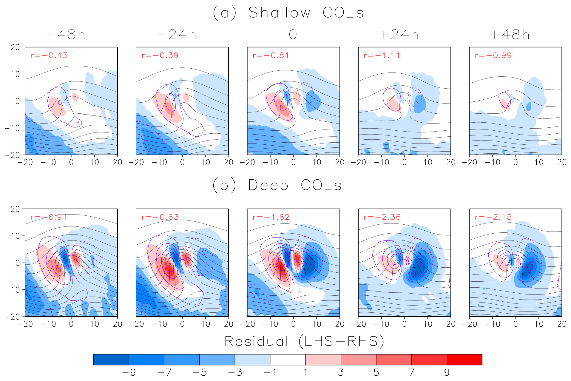
Figure 7Temporal evolution of the residual energy in joule (shaded), scaled by 109; geopotential height (black contour) at 300 hPa for contour intervals of 50 gpm; and vertical velocity (purple contour) for contour intervals of 0.05 Pa s−1, where the solid (dashed) contours indicate positive (negative) values. The red values represent the residual energy vertically averaged within a 15° spherical cap region centred on the COL location.
While negative residual energy prevails, it is worth noting that positive values emerge west of the COLs during the upper-level trough and tear-off stages. Conversely, negative residual energy is observed to the east of the COLs during the cut-off and decay stages. This contrasting pattern is particularly pronounced in deep COLs, consistent with previous findings on strong COLs (see Fig. 4 of Pinheiro et al., 2022).
The residual energy suggests the existence of development mechanisms that are either not considered in our approach or inadequately represented in the reanalysis data. A common issue lies in accurately representing diabatic processes, such as radiative cooling and latent heating, which poses challenges for reanalysis. A significant negative residual, particularly pronounced in deep COLs, is observed east of COLs where enhanced ascent and convection can introduce additional energy sources and unresolved phenomena contributing to the residual. In contrast, positive residual prevails along the western COL edge, possibly influenced by sinking air that promotes radiative cooling.
Uncertainties in measurement techniques, including inhomogeneous observations, analysis increment, and model parameterizations, are especially important in regions of intense convection. Although diabatic heating does not directly influence the EKE budget as it is not included in the energetic framework, errors in the reanalysis due to the misrepresentation of these processes (see https://confluence.ecmwf.int/display/FUG/Section+4.2+Analysis+Increments, last access: 24 June 2024) can lead to inconsistencies in the energetic analysis, as discussed by Pinheiro et al. (2022). Our results suggest that COLs that are more strongly dependent on diabatic processes are less well represented by reanalysis data. Additionally, the contribution of friction remains an unknown factor and is challenging to quantify directly. It is possible that stronger systems have a heightened residual contribution from frictional effects, although this remains an area of ongoing investigation.
This study has introduced a track matching algorithm applied to ERA-Interim reanalysis for accurate estimation of COL depth. Our findings highlight that the accuracy of COL depth estimation is primarily influenced by the temporal overlap (χ) between tracks at different pressure levels. We found that employing χ= 1 % with a mean separation distance of 5° geodesic provides a feasible approach for capturing COLs during specific lifecycle stages. Notably, our method reveals a lower proportion of deep COLs compared to previous studies (Porcù et al., 2007; Barnes et al., 2021). This discrepancy arises from differences in methods, where our vorticity-based approach detected a larger number of systems, leading to a relatively smaller frequency of deep COLs. However, vorticity-based identification offers advantages over geopotential data as it avoids subjective threshold adjustments across pressure levels and is more sensitive to weaker COLs, providing a more consistent method for analysing their vertical structure.
Further, we investigated the contrasting characteristics of COLs based on their vertical depth and intensity, categorizing them into four main types: shallow, deep, weak, and strong. Deep and strong COLs exhibit similar distribution patterns, predominantly concentrated in Australia and the southwestern Pacific. They are more intense and frequently found poleward of the subtropical jet, displaying a semiannual oscillation peaking in autumn and spring. In contrast, shallow and weak COLs are less intense, situated more equatorward and with increased frequencies in summer. However, despite these similarities, approximately 20 %–30 % of deep and shallow COLs align with the 50th percentile of the weakest and strongest systems, respectively. The variability within these classifications underscores the complexity inherent in COL dynamics, highlighting the need for future research to explore the interdependencies among these categories.
A particular novel aspect of our study is the differential impact of both subtropical and polar front jets on COLs. While COLs typically originate in regions characterized by weak zonal flow, the proximity of a jet streak is crucial for the system intensification and/or deepening. Our findings reveal that the COL deepening is more probable in the presence of a robust upstream polar front jet due to enhanced convergence of ageostrophic fluxes and baroclinic conversion, resulting in intensified vertical motions and a deeper cyclonic circulation. However, a stronger polar front jet does not necessarily correlate with more intense COLs.
Conversely, a positive correlation exists between COL intensity (both shallow and deep) and the subtropical jet, although this weakens when considering the seasonal cycle. This suggests limitations in using the annual cycle as a fixed factor. The COL intensification might be induced by the wind shear along the subtropical jet edge, which is supported by the observed small-scale jet stream equatorward of COLs (Ndarana et al., 2021). Nevertheless, uncertainties remain regarding the causal nature of this relationship. Further investigations employing causal inference methods (e.g. Samarasinghe et al., 2019; Docquier et al., 2024) could be employed to establish the cause-and-effect connections between COLs and jet streams.
Our findings suggest that the deepening process is also influenced by diabatic processes, which enhance vertical motions and lead to increased baroclinic conversion around the COLs. These processes contribute to longer lifetimes and greater interaction between mechanisms operating at different levels within deep COL systems. However, the misrepresentation of diabatic processes in reanalysis is a particular issue that affects the residual energy, leading to uncertainties. Negative residual energy dominated throughout the COL lifecycle, notably higher in deep systems. The presence of negative (positive) residual energy east (west) of the COLs points to the existence of dissipation (intensification) mechanisms not adequately represented in the reanalysis data, possibly related to latent heating (radiative cooling), as observed in Cavallo and Hakim (2010). Accurately representing diabatic processes in reanalyses is essential for maintaining consistency in the energetic analysis and understanding their role in deepening COLs. Therefore, it is crucial to re-evaluate COLs and the EKE budget whenever new reanalysis products such as ERA5 become available in future work.
In summary, our research emphasizes the importance of classifying COLs for understanding their key features and reveals their intricate relationships with jet streams. However, further development of the energetic framework, incorporating vertical ageostrophic fluxes as in Rivière et al. (2015), remains essential for comprehensively elucidating the eddy feedback mechanisms.
Table A1Sensitivity of the number of ξ300 COLs to time overlap for each pressure level (hPa), expressed as a percentage of the total number. The overlap thresholds are 1 %, 5 %, 10 %, 25 %, 50 %, 75 %, and 100 %.
The code used in this study is available upon request from the corresponding author for researchers interested in reproducing or extending the findings presented in the paper. The ERA-Interim reanalysis data were sourced from the ECMWF server.
The supplement related to this article is available online at: https://doi.org/10.5194/wcd-5-881-2024-supplement.
HRP: conceptualization, investigation, data curation, methodology, writing (original draft), visualization. KIH: software development, writing (review and editing). MAG: writing (review and editing).
The contact author has declared that none of the authors has any competing interests.
Publisher’s note: Copernicus Publications remains neutral with regard to jurisdictional claims made in the text, published maps, institutional affiliations, or any other geographical representation in this paper. While Copernicus Publications makes every effort to include appropriate place names, the final responsibility lies with the authors.
We would like to thank the Conselho Nacional de Desenvolvimento Científico e Tecnológico (CNPq; grant no. 151225/2023-0) and Fundação de Amparo à Pesquisa do Estado de São Paulo (FAPESP; grant no. 2023/10882-2) for their support and funding throughout this research. The authors have employed artificial intelligence (AI) to enhance the quality of the writing of an earlier version of this paper.
This research has been supported by the Conselho Nacional de Desenvolvimento Científico e Tecnológico (CNPq) (grant no. 151225/2023-0) and Fundação de Amparo à Pesquisa do Estado de São Paulo (FAPESP) (grant no. 2023/10882-2 (FAPESP)).
This paper was edited by Irina Rudeva and reviewed by two anonymous referees.
Bals-Elsholz, T. M., Atallah, E. H., Bosart, L. F., Wasula, T. A., Cempa, M. J., and Lupo, A. R.: The wintertime Southern Hemisphere split jet: Structure, variability, and evolution, J. Climate, 14, 4191–4215, 2001.
Barnes, M. A., Ndarana T., and Landman, W. A.: Cut-off lows in the Southern Hemisphere and their extension to the surface, Clim. Dynam., 56, 3709–3732, https://doi.org/10.1007/s00382-021-05662-7, 2021.
Bengtsson, L., Hodges, K. I., and Keenlyside, N.: Will extratopical storms intensify in a warmer climate?, J. Climate, 22, 2276–2301, https://doi.org/10.1175/2008JCLI2678.1, 2009.
Catto, J. L.: A new method to objectively classify extratropical cyclones for climate studies: Testing in the southwest Pacific region, J. Climate, 31, 4683–4704, https://doi.org/10.1175/JCLI-D-17-0746.1, 2018.
Cavallo, S. M. and Hakim, G. J.: Composite structure of tropopause polar cyclones, Mon. Weather Rev., 138, 3840–3857, https://doi.org/10.1175/2010MWR3371.1, 2010.
Davis, C. A. and Emanuel, K. A.: Potential vorticity diagnostics of cyclogenesis, Mon. Weather Rev., 119, 1929–1953, https://doi.org/10.1175/1520-0493(1991)119<1929:PVDOC>2.0.CO;2, 1991.
Dee, D. P., Uppala, S. M., Simmons, A. J., Berrisford, P., Poli, P., Kobayashi, S., Andrae, U., Balmaseda, M. A., Balsamo, G., Bauer, P., Bechtold, P., Beljaars, A. C. M., van de Berg, L., Bidlot, J., Bormann, N., Delsol, C., Dragani, R., Fuentes, M., Geer, A. J., Haimberger, L., Healy, S. B., Hersbach, H., Hólm, E. V., Isaksen, L., Kållberg, P., Köhler, M., Matricardi, M., McNally, A. P., Monge-Sanz, B. M., Morcrette, J. J., Park, B. K., Peubey, C., de Rosnay, P., Tavolato, C., Thépaut, J. N., and Vitart, F.: The ERA-Interim reanalysis: configuration and performance of the data assimilation system, Q. J. Roy. Meteor. Soc., 137, 553–597, https://doi.org/10.1002/qj.828, 2011.
Docquier, D., Di Capua, G., Donner, R. V., Pires, C. A. L., Simon, A., and Vannitsem, S.: A comparison of two causal methods in the context of climate analyses, Nonlin. Processes Geophys., 31, 115–136, https://doi.org/10.5194/npg-31-115-2024, 2024.
Favre, A., Hewitson, B., Tadross, M., Lennard, C., and Cerezo-Mota, R.: Relationships between cut-off lows and the semiannual and southern oscillations, Clim. Dynam., 38, 1473–1487, https://doi.org/10.1007/s00382-011-1030-4, 2012
Frank, N. L.: On the energetics of cold lows, in: Symposium on tropical meteorology, Proceedings American Meteorological Society EIV1–EIV6, Honolulu, 1970.
Deser, C., Magnusdottir, G., Saravanan, R., and Phillips, A.: The effects of North Atlantic SST and sea ice anomalies on the winter circulation in CCM3. Part II: Direct and indirect components of the response, J. Climate, 17, 5, 877–889, https://doi.org/10.1175/1520-0442(2004)017<0877:TEONAS>2.0.CO;2, 2004.
Gan, M. A. and Dal Piva, E.: Energetics of a southeastern Pacific cut-off low, Atmos. Sci. Lett., 14, 272–280, https://doi.org/10.1002/asl2.451, 2013.
Gan, M. A. and Dal Piva, E.: Energetics of southeastern Pacific cut-off lows, Clim. Dynam., 46, 3453–3462, https://doi.org/10.1007/s00382-015-2779-7, 2016.
Garreaud, R. D. and Fuenzalida, H. A.: The influence of the Andes on cutoff lows: a modeling study, Mon. Weather Rev., 135, 1596–1613, https://doi.org/10.1175/MWR3350.1, 2007.
Hodges, K. I. Feature tracking on the unit sphere. Mon. Weather Rev., 123, 3458–3465, https://doi.org/10.1175/1520-0493(1995)123<3458:FTOTUS>2.0.CO;2, 1995.
Hodges, K. I.: Spherical nonparametric estimators applied to the UGAMP model integration for AMIP, Mon. Weather Rev., 124, 2914–2932, https://doi.org/10.1175/1520-0493(1996)124<2914:SNEATT>2.0.CO;2, 1996.
Hodges, K. I.: Adaptive constraints for feature tracking, Mon. Weather Rev., 127, 1362–1373, https://doi.org/10.1175/1520-0493(1999)127<1362:ACFFT>2.0.CO;2, 1999.
Hodges, K. I., Boyle, J., Hoskins, B. J., and Thorncroft, C.: A comparison of recent reanalysis datasets using objective feature tracking: storm tracks and tropical easterly waves, Mon. Weather Rev., 131, 2012–2037, https://doi.org/10.1175/1520-0493(2003)131<2012:ACORRD>2.0.CO;2, 2003.
Hodges, K. I., Lee, R. W., and Bengtsson, L.: A comparison of extratropical cyclones in recent reanalyses ERAI, NASA MERRA, NCEP CFSR, and JRA-25, J. Climate, 24, 4888–4906, https://doi.org/10.1175/2011JCLI4097.1, 2011.
Hodges, K., Cobb, A., Vidale, P. L., Hodges, K., Cobb, A., and Vidale, P. L.: How well are tropical cyclones represented in reanalysis datasets?, J. Climate, 30, 5243–5264, https://doi.org/10.1175/JCLI-D-16-0557.1, 2017.
Hoskins, B. J. and Karoly, D. J.: The steady linear response of a spherical atmosphere to thermal and orographic forcing, J. Atmos. Sci., 38, 1179–1196, https://doi.org/10.1175/1520-0469(1981)038<1179:TSLROA>2.0.CO;2, 1981
Kushner, P. J., Held, I. M., and Delworth, T. L.: Southern Hemisphere atmospheric circulation response to global warming, J. Climate, 14, 2238–2249, https://doi.org/10.1175/1520-0442(2001)014<0001:SHACRT>2.0.CO;2, 2001
Lakkis, S. G., Canziani, P., Yuchechen, A., Rocamora, L., Caferri, A., Hodges, K., and O'Neill, A.: A 4D feature-tracking algorithm: a multidimensional view of cyclone systems, Q. J. Roy. Meteor. Soc., 145, 395–417, https://doi.org/10.1002/qj.3436, 2019.
Lim, E. P. and Simmonds, I.: Southern Hemisphere winter extratropical cyclone characteristics and vertical organization observed with the ERA-40 data in 1979–2001, J. Climate, 20, 2675–2690, https://doi.org/10.1175/JCLI4135.1, 2007.
Llasat, M. C., Martín, F., and Barrera, A.: From the concept of “Kaltlufttropfen” (cold air pool) to the cut-off low. The case of September 1971 in Spain as an example of their role in heavy rainfalls, Meteorol. Atmos. Phys., 96, 43–60, https://doi.org/10.1175/JCLI-D-16-0557.1, 2007.
Lu, J., Sun, L., Wu, Y., and Chen, G.: The role of subtropical irreversible PV mixing in the zonal mean circulation response to global warming–like thermal forcing, J. Climate, 27, 2297–2316, https://doi.org/10.1175/JCLI-D-13-00372.1, 2014
McInnes, K. L. and Hubbert, G. D.: The impact of eastern Australian cut-off lows on coastal sea levels, Meteorol. Appl., 8, 229–244, https://doi.org/10.1017/S1350482701002110, 2001.
Nakamura, H.: Midwinter suppression of baroclinic wave activity in the Pacific, J. Atmos. Sci., 49, 1629–1642, https://doi.org/10.1175/1520-0469(1992)049<1629:MSOBWA>2.0.CO;2, 1992.
Muñoz, C., Schultz, D., Vaughan, G.: A midlatitude climatology and interannual variability of 200 and 500 hPa cut-off lows, J. Climate, 33, 2201–2222, 2020.
Ndarana, T. and Waugh, D. W.: The link between cut-off lows and Rossby wave breaking in the Southern Hemisphere, Q. J. Roy. Meteor. Soc., 136, 869–885, 2010.
Ndarana, T., Rammopo, T. S., Chikoore, H., Barnes, M. A., and Bopape, M. J.: A quasi-geostrophic diagnosis of the zonal flow associated with cut-off lows over South Africa and surrounding oceans, Clim. Dynam., 55, 2631–2644, https://doi.org/10.1007/s00382-020-05401-4, 2020.
Ndarana, T., Rammopo, T. S., Bopape, M. J., Reason, C. J., and Chikoore, H.: Downstream development during South African cut-off low pressure systems, Atmos. Res., 249, 105315, https://doi.org/10.1016/j.atmosres.2020.105315, 2021.
Nie, Y., Zhang, Y., Chen, G., and Yang, X. Q.: Delineating the barotropic and baroclinic mechanisms in the midlatitude eddy-driven jet response to lower-tropospheric thermal forcing, J. Atmos. Sci., 73, 429–448, https://doi.org/10.1175/JAS-D-15-0090.1, 2016.
Nieto, R., Gimeno, L., Torre, L. D. L., Ribera, P., Gallego, D., García, J. A., Nunez, M., Redano, A., and Lorente, J.: Climatological features of cutoff low systems in the Northern Hemisphere, J. Climate, 18, 3085–3103, https://doi.org/10.1175/JCLI3386.1, 2005.
Nieto, R., Sprenger, M., Wernli, H., Trigo, R. M., and Gimeno, L.: Identification and climatology of cut-off lows near the tropopause, Ann. NY Acad. Sci., 1146, 256–290, https://doi.org/10.1196/annals.1446.016, 2008.
Orlanski, I. and Katzfey, J.: The life cycle of a cyclone wave in the Southern Hemisphere: eddy energy budget, J. Atmos. Sci., 48, 1972–1998, https://doi.org/10.1175/1520-0469(1991)048<1972:TLCOAC>2.0.CO;2, 1991.
Palmén, E.: Origin and structure of high-level cyclones south of the maximum westerlies, Tellus, 1, 22–31, https://doi.org/10.1111/j.2153-3490.1949.tb01925.x, 1949.
Pezzulli, S., Stephenson, D. B., and Hannachi, A.: The variability of seasonality, J. Climate, 18, 71–88, 2005.
Pinheiro, H. R., Hodges, K. I., Gan, M. A., and Ferreira, N. J.: A new perspective of the climatological features of upper-level cut-off lows in the Southern Hemisphere, Clim. Dynam., 48, 541–559, https://doi.org/10.1007/s00382-016-3093-8, 2017.
Pinheiro, H. R., Hodges, K. I., and Gan, M. A.: Sensitivity of identifying Cut-off Lows in the Southern Hemisphere using multiple criteria: implications for numbers, seasonality and intensity, Clim. Dynam., 53, 6699–6713, https://doi.org/10.1007/s00382-019-04984-x, 2019.
Pinheiro, H. R., Hodges, K. I., and Gan, M. A.: An intercomparison of Cut-off Lows in the subtropical Southern Hemisphere using recent reanalyses: ERA-Interim, NCEP-CFSR, MERRA-2, JRA-55, and JRA-25, Clim. Dynam., 54, 777–792, https://doi.org/10.1007/s00382-019-05089-1, 2020.
Pinheiro, H. R., Gan, M. A., and Hodges, K. I.: Structure and evolution of intense austral Cut-off Lows, Q. J. Roy. Meteor. Soc., 147, 1–20, https://doi.org/10.1002/qj.3900, 2021.
Pinheiro, H. R., Hodges, K. I., Gan, M. A., Ferreira, S. H., and Andrade, K. M.: Contributions of downstream baroclinic development to strong Southern Hemisphere cut-off lows, Q. J. Roy. Meteor. Soc., 148, 214–232, https://doi.org/10.1002/qj.4201, 2022.
Pinto, J. R. D. and da Rocha, R. P.: The energy cycle and structural evolution of cyclones over southeastern South America in three case studies, J. Geophys. Res., 116, 1–17, https://doi.org/10.1029/2011JD016217, 2011.
Porcù, F., Carrassi, A., Medaglia, C. M., Prodi, E., and Mugnai, A.: A study on cut-off low vertical structure and precipitation in the Mediterranean region, Meteorol. Atmos. Phys., 96, 121–140, https://doi.org/10.1007/s00703-006-0224-5, 2007.
Portmann, R., Crezee, B., Quinting, J., and Wernli, H.: The complex life cycles of two long-lived potential vorticity cut-offs over Europe, Q. J. Roy. Meteor. Soc., 144, 701–719, https://doi.org/10.1002/qj.3239, 2018.
Portmann, R., Sprenger, M., and Wernli, H.: The three-dimensional life cycles of potential vorticity cutoffs: a global and selected regional climatologies in ERA-Interim (1979–2018), Weather Clim. Dynam., 2, 507–534, https://doi.org/10.5194/wcd-2-507-2021, 2021.
Ring, M. J. and Plumb, R. A.: Forced annular mode patterns in a simple atmospheric general circulation model, J. Atmos. Sci., 64, 3611–3626, https://doi.org/10.1175/JAS4031.1, 2007.
Rivière, G., Arbogast, P., and Joly, A.: Eddy kinetic energy redistribution within windstorms Klaus and Friedhelm, Q. J. Roy. Meteor. Soc., 141, 925–938, https://doi.org/10.1002/qj.2412, 2015.
Sakamoto, K. and Takahashi, M.: Cut off and weakening processes of an upper cold low, J. Meteorol. Soc. Jpn., 83, 817–834, https://doi.org/10.2151/jmsj.83.817, 2005.
Samarasinghe, S. M., McGraw, M. C., Barnes, E. A., and Ebert-Uphoff, I.: A study of links between the Arctic and the midlatitude jet stream using Granger and Pearl causality, Environmetrics, 30, e2540, https://doi.org/10.1002/env.2540, 2019.
Simmonds, I. and Jones, D. A.: The mean structure and temporal variability of the semiannual oscillation in the southern extratropics, Int. J. Climatol., 18, 473–504, 1998.
Sinclair, M. R. and Revell, M. J: Classification and composite diagnosis of extratropical cyclogenesis events in the southwest Pacific, Mon. Weather Rev., 128, 1089–1105, https://doi.org/10.1175/1520-0493(2000)128<1089:CACDOE>2.0.CO;2, 2000.
Singleton, A. T. and Reason, C. J. C.: A numerical model study of an intense cutoff low pressure system over South Africa, Mon. Weather Rev., 135, 1128–1150, https://doi.org/10.1175/MWR3311.1, 2007.
Stoelinga, M. T.: A potential vorticity-based study of the role of diabatic heating and friction in a numerically simulated baroclinic cyclone, Mon. Weather Rev., 124, 849–874, https://doi.org/10.1175/1520-0493(1996)124<0849:APVBSO>2.0.CO;2, 1996.
Trenberth, K. E.: Storm tracks in the Southern Hemisphere, J. Atmos. Sci., 48, 2159–2178, https://doi.org/10.1175/1520-0469(1991)048<2159:STITSH>2.0.CO;2, 1991.
Van Loon, H.: The half-yearly oscillations in middle and high southern latitudes and the coreless winter, J. Atmos. Sci., 24, 472–486, 1967.