Model spread in multidecadal North Atlantic Oscillation variability connected to stratosphere–troposphere coupling

The underestimation in multidecadal variability in the wintertime North Atlantic Oscillation (NAO) by global climate models remains poorly understood. Understanding the origins of this weak NAO variability is important for making model projections more reliable. Past studies have linked the weak multidecadal NAO variability in models to an underestimated atmospheric response to the Atlantic Multidecadal Variability (AMV). We investigate historical simulations from Coupled Model Intercomparison Project Phase 6 (CMIP6) large-ensemble models and find that most of the models do not reproduce observed multidecadal NAO variability, as found in previous generations of climate models. We explore statistical relationships with physical drivers that may contribute to inter-model spread in NAO variability. There is a significant anticorrelation across models between the AMV–NAO coupling parameter and multidecadal NAO variability over the full historical period ($r=-\mathrm{0.55}$, p<0.05). However, this relationship is relatively weak and becomes obscured when using a common period (1900–2010) and de-trending the data in a consistent way, with observations to enable a model–data comparison. This suggests that the representation of NAO–AMV coupling contributes to a modest proportion of inter-model spread in multidecadal NAO variability, although the importance of this process for model spread could be underestimated, given evidence of a systematically poor representation of the coupling in the models. We find a significant inter-model correlation between multidecadal NAO variability and multidecadal stratospheric polar vortex variability and a stratosphere–troposphere coupling parameter, which quantifies the relationship between stratospheric winds and the NAO. The models with the lowest NAO variance are associated with weaker polar vortex variability and a weaker stratosphere–troposphere coupling parameter. The two stratospheric indices are uncorrelated across models and together give a pooled R² with an NAO variability of 0.7, which is larger than the fraction of inter-model spread related to the AMV (R²=0.3). The identification of this relationship suggests that modelled spread in multidecadal NAO variability has the potential to be reduced by improved knowledge of observed multidecadal stratospheric variability; however, observational records are currently too short to provide a robust constraint on these indices.

1 Introduction

The North Atlantic Oscillation (NAO) is the dominant mode of atmospheric circulation variability in the North Atlantic sector in winter and exerts a strong influence on regional weather and climate, especially over Europe and the US (Hurrell et al., 2003). A positive NAO phase is associated with a stronger meridional pressure gradient between the North Atlantic subtropical anticyclone and the Icelandic Low, leading to a stronger North Atlantic eddy-driven jet stream and a northward displacement of the storm track. In winter, this brings mild and wet weather to northern Europe and cold and dry weather to southern Europe.

Projections of wintertime surface climate over Europe depend on reliable simulation of the NAO (e.g. McKenna and Maycock, 2022). Several studies have shown that coupled climate models underestimate decadal-to-multidecadal NAO variability (e.g. Bracegirdle, 2022; Kravtsov, 2017; Wang et al., 2017; Kim et al., 2018; Eade et al., 2022) and North Atlantic jet strength variability (Bracegirdle et al., 2018; Simpson et al., 2018). It has been proposed that the too-low multidecadal North Atlantic atmospheric variability is related to simulated North Atlantic sea surface temperature (SST) variations and an underestimation by models of the atmospheric response to SST variability through too-weak air–sea coupling (Kim et al., 2018; Bracegirdle, 2022; Simpson et al., 2018).

Another important mechanism that influences winter NAO variability is the stratospheric polar vortex strength and the related coupling between the stratosphere and troposphere. On average, a weaker polar vortex leads to a negative winter NAO anomaly and vice versa (Baldwin and Dunkerton, 2001). Low-frequency polar vortex variability has been implicated in decadal surface climate trends (Garfinkel et al., 2018; Kretschmer et al., 2018; Zhang et al., 2016; Butler et al., 2023). A recent study from Zhao et al. (2022) highlighted a bias towards a weak polar vortex in the lower stratosphere in most of the CMIP6 climate models. Those models also have a large diversity in the representation of intra-seasonal and interannual variability in the polar vortex (Charlton-Perez et al., 2013; Hall et al., 2021). However, the characteristics of multidecadal polar vortex variability in climate models are relatively understudied, in part because there are poor observational constraints due to the too-short record of stratospheric data.

The global tropics are also an important driver of the winter NAO, with myriad teleconnections emerging at sub-seasonal-to-seasonal (S2S) timescales from modes like the El Niño – Southern Oscillation (ENSO; Ineson and Scaife, 2009), the Madden–Julian Oscillation (MJO; Cassou, 2008) and Indian Ocean Dipole (IOD; Hardiman et al., 2020) and at decadal timescales from the Interdecadal Pacific Oscillation (IPO; Seabrook et al., 2023). While it has been suggested that tropical Pacific teleconnections to the NAO are too weak at seasonal timescales (Williams et al., 2023), the role of tropical forcing of the NAO at multidecadal timescales and the extent to which this may contribute to the underestimated NAO variability in models remain unclear.

Recent work has suggested a relationship between the NAO response to external drivers and the modelled relationship between eddy momentum fluxes and the extratropical zonal wind, a so-called “eddy feedback parameter” (e.g. Smith et al., 2022; Hardiman et al., 2022; Screen et al., 2022). However, the extent to which eddy–mean flow interactions may be linked to poor simulation of the large-scale circulation at multidecadal timescales is unclear.

Understanding the origin of the weak multidecadal NAO variability in models is important for resolving biases in climate models and making projections more reliable. In this paper, we further investigate the underestimation of the winter NAO multidecadal variability within the Coupled Model Intercomparison Project Phase 6 (CMIP6) models by testing the extent to which the aforementioned mechanisms can explain the spread across climate models in their simulated NAO multidecadal variability.

The paper is organised as follows. The datasets, climate indices and statistical methods used are described in Sect. 2. The multidecadal NAO variability within the CMIP6 multi-model ensemble is then evaluated in Sect. 3. Section 4 analyses the origin of the spread in multidecadal NAO variability across the CMIP6 multi-model ensemble, highlighting the role of the polar vortex strength variability. Then, the origin of the spread in polar vortex strength variability within the CMIP6 multi-model ensemble is investigated. Finally, the main limitations of this study are discussed, and conclusions and perspectives are drawn in Sect. 5.

2 Data and methods

2.1 Datasets

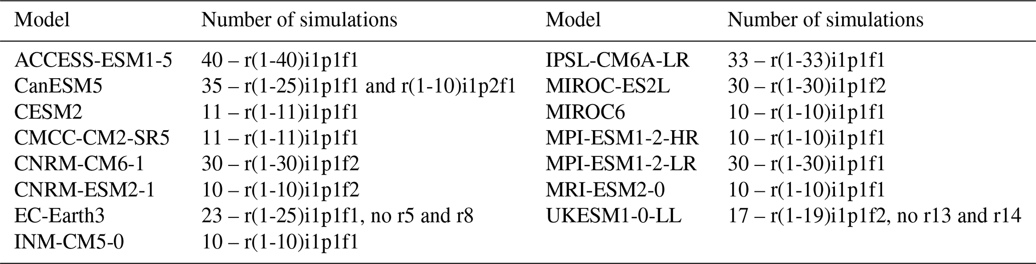
Historical simulations from 15 CMIP6 models (Eyring et al., 2016) are used in this study (Table 1). Analysing drivers of low-frequency climate variability requires long simulations to find physical relationships and to reduce the likelihood of spurious correlations due to poor sampling. Therefore, we analyse CMIP6 models providing at least 10 ensemble members for the Diagnostic, Evaluation and Characterization of Klima (DECK) historical experiment with the daily zonal wind (ua) and meridional wind (va) variables that are needed to calculate the eddy feedback parameter described in Sect. 1 (see Sect. 2.2.5). Note that some models have additional ensemble members in the Earth System Grid Federation (ESGF) that are not included here because they did not provide daily wind data at the time of analysis. All atmospheric data are regridded to the horizontal resolution of the Canadian Earth System Model version 5 (CanESM5), which is the coarsest model grid, using bilinear interpolation. The sea surface temperature (SST) data are regridded over a regular 1°×1° grid using bilinear interpolation. We tested the sensitivity of the results to the regridding by recalculating the analysis using the native resolutions of the datasets and find that this does not affect the results shown in the paper.

Table 1 Summary of the 15 CMIP6 models and the associated number and list of DECK historical simulations used in this study.

Since our focus is on multidecadal variability, to estimate observed NAO variability we use two long-term atmospheric reanalyses: the NOAA-CIRES-DOE 20th Century Reanalysis V3 (20CRv3; Slivinski et al., 2019) and the ECMWF Reanalysis of the 20th Century (ERA20C; Poli et al., 2016), as well as the Hadley Centre Sea Level Pressure dataset (HadSLP2r; Allan and Ansell, 2006). Two long-term observational datasets of SST are also used: the Hadley Centre Sea Ice and Sea Surface Temperature dataset (HadISST; Rayner et al., 2003) and the NOAA Extended Reconstructed SST V5 (ERSSTv5; Huang et al., 2017). We analyse the observation-based datasets over the common period of 1900–2010. It is important to recognise that the characterisation of low-frequency variability in instrumental datasets is rather limited due to the low degrees of freedom. Therefore, when evaluating the large-ensemble model simulations, we ask where the observations lie within the ensemble spread to determine the likelihood that a model is biased (Maher et al., 2021).

The analysis focuses on the extended December-to-March winter period, since several recent studies point out that the underestimation of North Atlantic atmospheric variability, including the NAO, is also present in March (Simpson et al., 2018; Bracegirdle, 2022).

2.2 Climate indices

2.2.1 NAO index

Following Stephenson et al. (2006) and Baker et al. (2018), the NAO index is defined as the difference in area-averaged mean sea level pressure (MSLP) between a southern box (20–55° N, 90° W–60° E) and a northern box (55–90° N, 90° W–60° E) in the North Atlantic. We chose this index because it is less sensitive to modest differences in NAO centres of action between the observations and the CMIP6 models than the station-based index is (Hurrell et al., 2003; Stephenson et al., 2006). Another benefit of this index is that it is less affected by issues of interpretability that occur when using a mathematically constructed empirical orthogonal function (EOF)-based index (Ambaum et al., 2001; Dommenget and Latif, 2002; Stephenson et al., 2006).

2.2.2 AMV definition

The Atlantic Multidecadal Variability (AMV) is the leading mode of multidecadal variability in the North Atlantic Ocean and is characterised by basin-wide SST variations (Schlesinger and Ramankutty, 1994; Enfield et al., 2001; Yeager and Robson, 2017). To estimate the evolution of the AMV, the AMV index is generally defined as the average SST over the North Atlantic (0–60° N, 80° W–0° E) after the removal of the externally forced signal. A low-pass filter is then used to retain only the low-frequency variations. The most accurate way to estimate the external forcing from climate simulations is to use the ensemble mean when enough simulations are available (Deser et al., 2020). However, this is not possible for the observations. Therefore, we also use the Trenberth and Shea (2006) method (TS2006 hereafter), which estimates the effect of external forcings by removing the global averaged SST between 60° S and 60° N from North Atlantic SST, although other methods can be used (Qasmi et al., 2017).

2.2.3 Interdecadal Pacific Oscillation definition

The Interdecadal Pacific Oscillation (IPO) is characterised by a horseshoe pattern of SST variability over the North Pacific. A positive phase of the IPO is associated with an eastern warming and a cooling in the Kuroshio–Oyashio Extension similar to the Pacific Decadal Oscillation pattern: a warming over the tropical Pacific region and a cooling over the southwestern Pacific Ocean (Newman et al., 2016). We use the tripole index (TPI) to estimate the IPO (Henley et al., 2015), which is the weighted difference between de-seasonalised monthly SST anomalies (SSTA) over the central equatorial Pacific (SSTA₂; 10° S–10° N, 170° E–90° W), the northwest (SSTA₁; 25–45° N, 140° E–145° W) and the southwest Pacific (SSTA₃; 50–15° S, 150° E–160° W): TPI = SSTA₂−(SSTA₁-SSTA${}_{\mathrm{3}})/\mathrm{2}$.

2.2.4 Polar vortex strength

To estimate the multidecadal variability in the stratospheric polar vortex, we calculate the variance of the 20-year running mean extended winter (DJFM) zonal mean zonal wind averaged between 60–70° N at 50 hPa (Castanheira and Graf, 2003; Walter and Graf, 2005).

Sudden stratospheric warmings (SSWs) are a key feature of the Northern Hemisphere polar vortex, during which the vortex rapidly breaks down and typically recovers over a period of weeks to months. Past work has identified multidecadal variability in SSW frequency (Dimdore-Miles et al., 2022). To identify SSWs, we use the index of Charlton and Polvani (2007) based on the temporary reversal of zonal mean zonal wind at 60° N and 10 hPa between the months of December and March. To be considered discrete SSW events, periods of wind reversal (to easterly) must be separated by at least 20 consecutive days of westerly winds. We calculate the 20-year running mean winter SSW frequency and examine whether multidecadal variability in winter polar vortex strength is related to variability in SSW frequency (e.g. Jucker et al., 2014).

2.2.5 Eddy feedback parameter

To quantify the so-called eddy feedback parameter (EFP) we follow Hardiman et al. (2022). From the daily zonal (u) and meridional (v) winds at 500 hPa, we compute the zonal acceleration due to the quasi-geostrophic component of the horizontal EP-flux divergence (Andrews et al., 1987),

$$\begin{array}{}\text{(1)}& {\displaystyle \frac{\mathrm{\nabla }.F_h}{\mathit{\rho }a\cos \mathit{\varphi }}}={\displaystyle \frac{-\mathrm{1}}{a{\cos }^{\mathrm{2}}\mathit{\varphi }}}{\displaystyle \frac{\mathrm{d}\left(\stackrel{\mathrm{‾}}{u{}^{\prime }v{}^{\prime }}{\cos }^{\mathrm{2}}\mathit{\varphi }\right)}{\mathrm{d}\mathit{\varphi }}},\end{array}$$

where ρ is density, ϕ is latitude, a is the Earth's radius, overbars represent a zonal mean and primes represent the residual after removing the zonal mean. The extended winter mean is then calculated from the daily values of this zonal acceleration. In parallel, the extended winter mean of the zonal mean zonal wind ($\overline{u}$) is computed for each year. Next, the time correlation is calculated at each latitude between the zonal acceleration and the zonal mean zonal wind ($\overline{u}$). Finally, the eddy feedback parameter is calculated as the area-weighted average of this correlation squared over 25–72° N. It is important to note that the EFP does not formally represent the feedback of eddies into the mean flow (e.g. Lorenz and Hartmann, 2001), rather it reflects the cross-correlation between EP-flux divergence and zonal wind.

2.3 Statistical methods

Our analysis focuses on explaining the inter-model spread of multidecadal NAO variability in the CMIP6 multi-model ensemble. To estimate the error in the ensemble mean variance (μ) and the possibly related variables for each CMIP6 model, two-sided confidence intervals are calculated as $\mathit{\mu }\pm \mathit{\sigma }/N$, where σ is the standard deviation across N ensemble members (Storch and Zwiers, 1999). To test the significance of the relationship between two variables, the p value is provided from a two-tailed Wald test with a null hypothesis that the slope is zero.

3 Evaluation of simulated winter NAO variability

We first evaluate the representation of historical multidecadal winter NAO variability in the CMIP6 large ensembles compared to the observation-based datasets. Figure 1 shows the winter NAO index for the three observation-based MSLP datasets. While there are similar inter-decadal variations in the datasets, there are discrepancies in the apparent long-term trends. There is almost no long-term trend in HadSLP2r over this period, whereas there is a positive linear trend of 1.49 and 1.38 hPa per century in the ERA20C and the 20CRv3 reanalyses, respectively. This trend leads to larger multidecadal variability in those datasets compared to HadSLP2r (Fig. 1a). Studies have highlighted potential unrealistic trends in long-term reanalyses (Krueger et al., 2013; Oliver, 2016) because only a limited set of surface observations are assimilated (sea level pressure and surface wind for ERA20C), and the density of the observation network evolves with time. HadSLP2r is based on station observations whose density also changes through time. Therefore, given the differences in composition of the datasets, it is difficult to assess the validity of their long-term NAO trends. De-trending the datasets results in a closer evolution of the multidecadal NAO and the associated multidecadal variance (Fig. 1b). At multidecadal timescales, an apparent long-term trend may reflect externally forced changes but may also be affected by the phasing of internal variability relative to the trend end points. Therefore, de-trending may remove some of the unforced variability we are interested in. Nevertheless, given the differences amongst datasets, unless otherwise stated, the remaining analyses for observations and models use linearly de-trended time series for all variables.

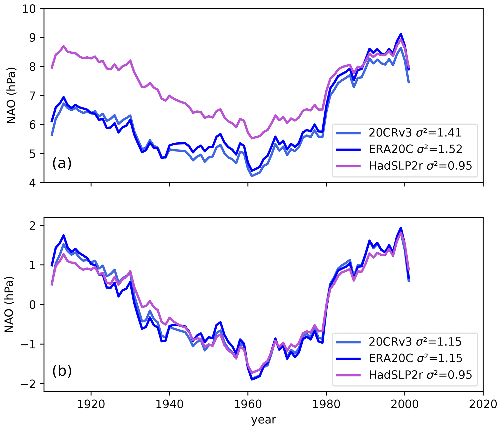
Figure 1 (a) Evolution of the extended winter (DJFM) NAO for the 20CRv3 reanalysis, the ERA20C reanalysis and the HadSLP2r Sea Level Pressure dataset over their common period (1900–2010). (b) Same as (a) but with the 1900–2010 linear trend removed. A running mean with a 20-year window is applied to each dataset. The variance σ² calculated over the whole period for each dataset is given in the legend.

The variance in the 20-year running mean NAO in the observation-based datasets lies within the extreme upper range of the CMIP6 model distributions, with only a few realisations having variances above or close to what was observed (Fig. 2). As the variance of the HadSLP2r dataset is 17 % lower than the two reanalyses, this dataset is somewhat more consistent with the CMIP6 simulations, although it is still within the very top of the range. Most of the models have no simulations close to the observed variance. This underestimation is still visible but is lower when using a 10-year running mean NAO for the ERA20C and 20CRv3 reanalyses (Fig. S1 in the Supplement). For HadSLP2r, the underestimation is even smaller and is not visible for some models, although some of them still fail to reproduce the variability. This quasi-systematic underestimation of the multidecadal NAO variance by CMIP6 models has also been highlighted in recent studies (e.g. Schurer et al., 2023). The fact that very few simulations are able to reproduce the observed variability suggests that a bias is present in climate models. However, it is possible, albeit unlikely, that the observations are characterised by a very high low-frequency internal variability by chance.

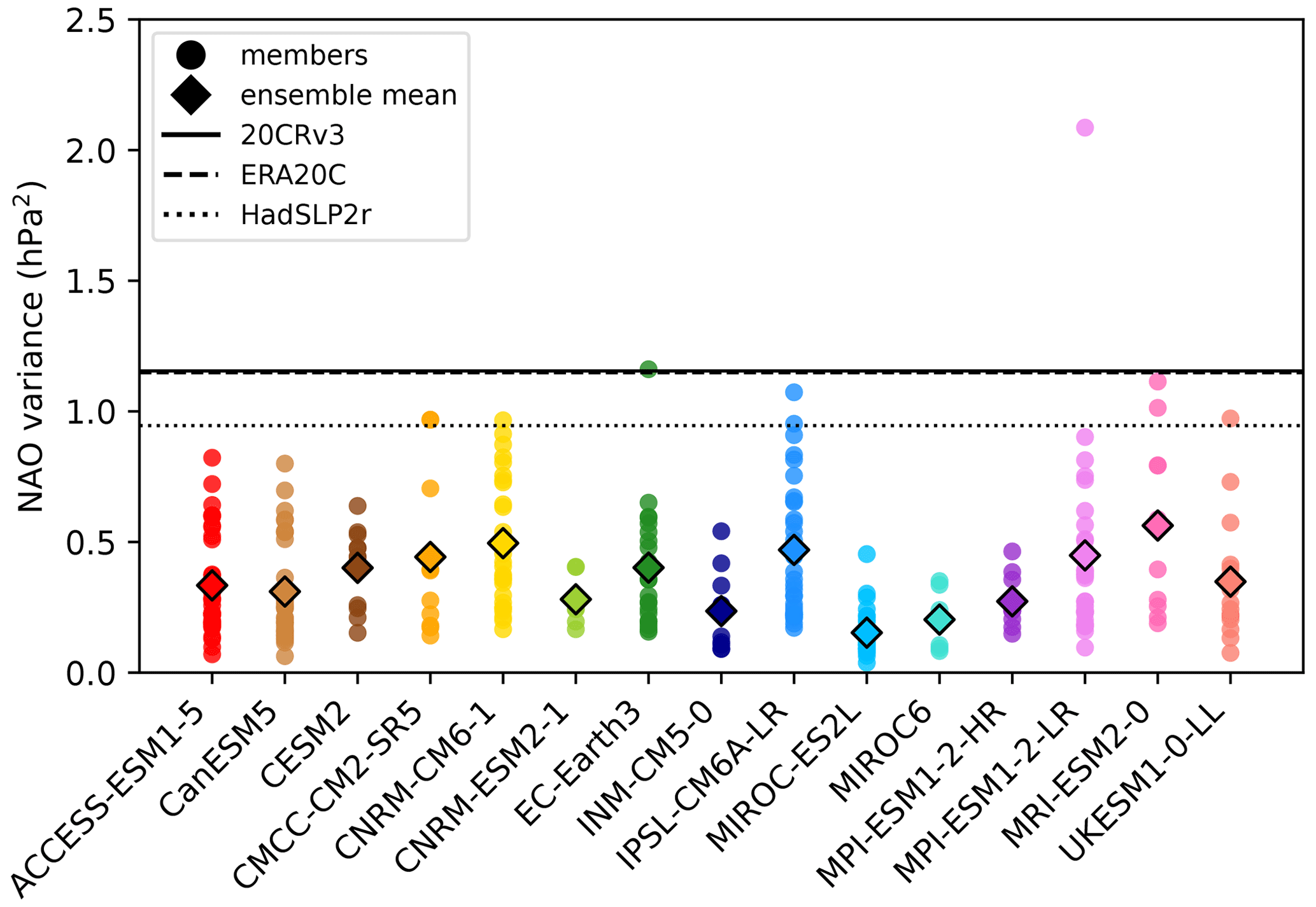
Figure 2 December-to-March de-trended 20-year running mean NAO variance (hPa²) for each member of the 15 CMIP6 ensembles (dots), the ensemble mean (diamonds) and the three observation-based datasets: 20CRv3 (solid line), ERA20C (dashed line) and HadSLP2r (dotted line) calculated over the 1900–2010 period.

While the systematic underestimation of multidecadal NAO variance compared to observations is clear in Fig. 2, there are also differences in variance between individual models. The ensemble mean low-frequency NAO variance in Fig. 2 varies by up to around a factor of 3, from 0.15 to 0.57 hPa². In order to identify some of the factors that may influence the representation of low-frequency NAO variance in models, for the remainder of the study we focus on exploring the inter-model spread in ensemble mean NAO variance and its relationship to other climate parameters. For consistency with observations, we focus on the 1900–2010 period and use de-trended time series of climate parameters.

4 Origins of the inter-model spread in multidecadal winter NAO variability in CMIP6

4.1 Relationship of NAO variability to Atlantic Multidecadal Variability

We first evaluate the relationship amongst models between low-frequency NAO variance and the simulated AMV variance. It has been shown that a negative NAO phase follows a positive AMV phase in both observations (Peings and Magnusdottir, 2014; Gastineau and Frankignoul, 2015) and in simulations from CMIP5 models (Gastineau et al., 2013; Peings et al., 2016) as well as in some CMIP6 models (Ruggieri et al., 2021; Börgel et al., 2022). These findings suggest positive feedback between the AMV and the NAO, with positive SST anomalies in the North Atlantic leading to a negative NAO phase that subsequently reinforces the positive AMV and vice versa. Such coupled feedback would enhance the total low-frequency NAO variability (e.g. Farneti and Vallis, 2011). Therefore, an underestimation of AMV variability and/or the coupling between the AMV and the overlying atmospheric circulation could introduce deficiencies in the NAO variability (Bracegirdle, 2022).

There is substantial diversity in simulated AMV in the CMIP6 models, with different magnitudes (Fig. 3) and periodicities (Fig. S2). Some models are characterised by larger ensemble mean AMV variability and larger ensemble spread that encompasses the observations (CMCC-CM2-SR5, CNRM-CM6-1, CNRM-ESM2-1, EC-Earth3 and IPSL-CM6A-LR), potentially overestimating the variability (e.g. EC-Earth3), while others have very weak average AMV variability and smaller ensemble spread (INM-CM5-0, MIROC-ES2L, MIROC6 and MPI-ESM1-2-LR). Despite the spread in AMV representation across models, no significant relationship is found between the ensemble mean variance of the NAO and the AMV over the 1900–2010 period (Fig. 4). This is also the case when using 10- or 30-year running means, as well as when considering the whole historical period of 1850–2014 (not shown).

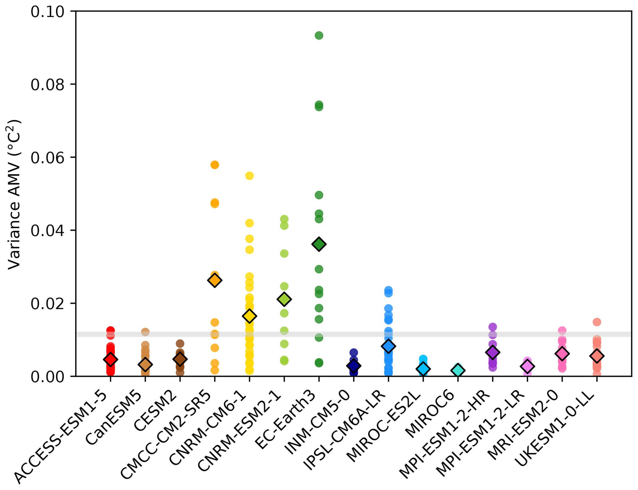
Figure 3 December-to-March 20-year running mean AMV variance (°C²) for individual members (dots), the ensemble means (diamonds) and two observational datasets, HadISST and ERSSTv5 (shaded grey bar), calculated over 1900–2010.

While there is no relationship between the total NAO and AMV variances across models, there may be differences in the coupling parameters between the multidecadal NAO and AMV. We evaluate the coupling between the AMV and the NAO using the linear regression slope between the 20-year running mean NAO and AMV time series in each ensemble member (Fig. 5). A large range of apparent NAO–AMV coupling amplitudes are found in individual members, with simulations with a strong positive relationship and others with a strong negative relationship, even within the same climate model (Fig. 5a). The observed NAO–AMV regression slope is on the more negative end of the range of all the simulations. This could mean either that the atmosphere–ocean coupling is biased in the models or that the observations by chance exhibit a strong negative relationship between the AMV and NAO. Figure 5a reflects the instantaneous relationship between the NAO and AMV: when the AMV leads the NAO, the underestimation of the relationship compared to observations is even larger (Fig. 5b). Conversely, when the NAO leads the AMV, the observed coupling between the AMV and the NAO is closer to the simulated range. This suggests that the atmosphere forcing the ocean may be better simulated than the ocean forcing the atmosphere.

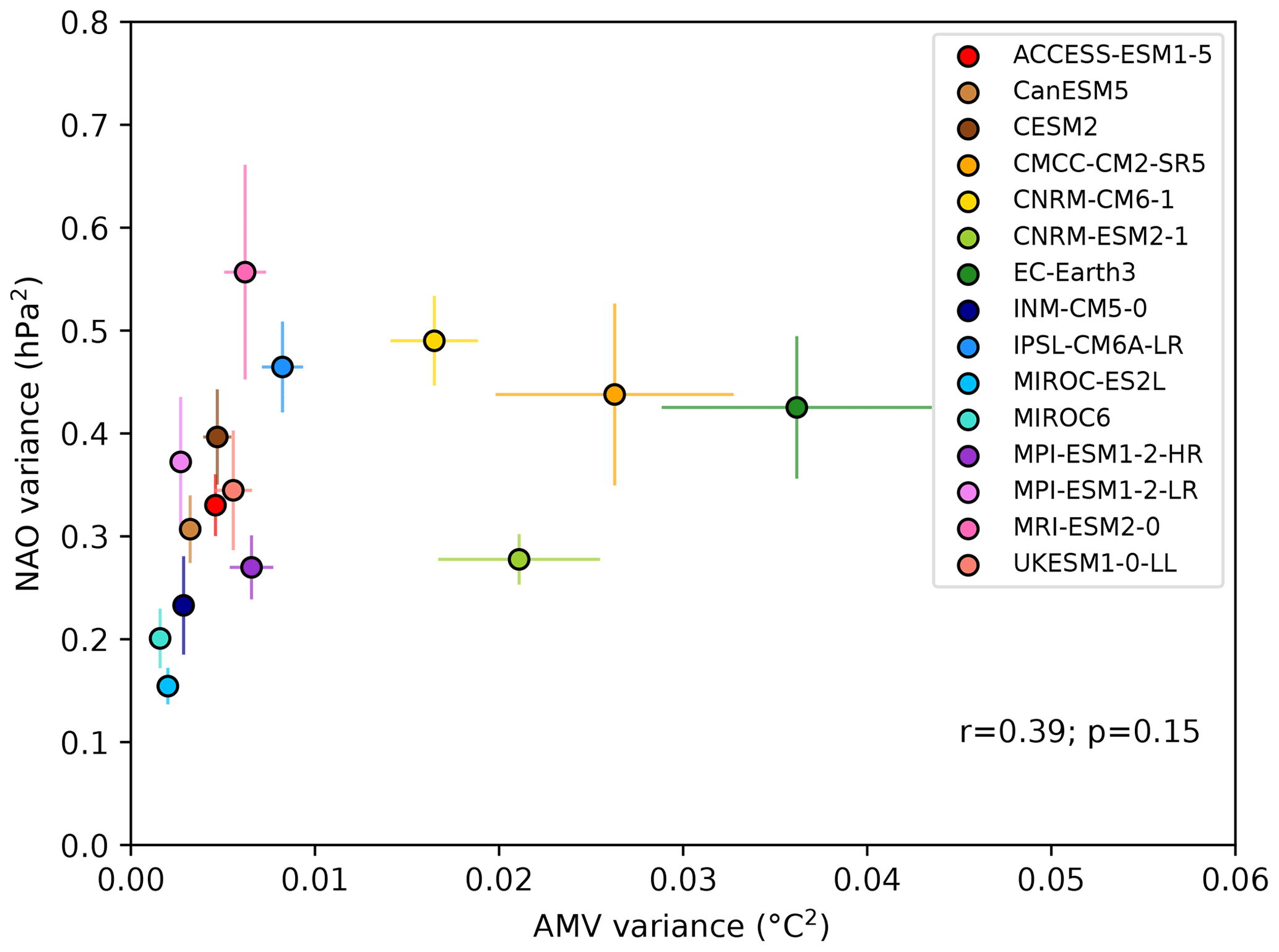
Figure 4 Scatter plot of the ensemble mean 20-year running mean NAO variance (hPa²) versus the 20-year running mean AMV index variance (°C²) in each model for DJFM over 1900–2010.

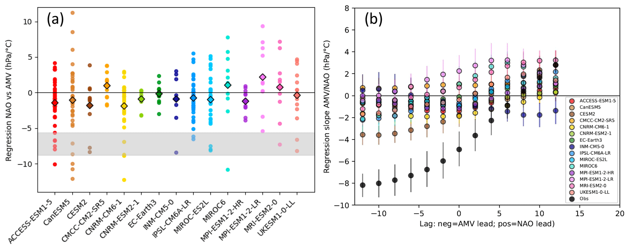
Figure 5 (a) Regression slope between the 20-year running mean NAO and AMV indices for DJFM over 1900–2010 for each model ensemble member (dots) and the ensemble mean of these regressions (diamonds). The observed range of the regression slope (grey area) is defined as the minimum and maximum of the slopes calculated from all permutations of the observational datasets (HadISST and ERSSTv5 for the AMV and 20CRv3, ERA20C and HadSLP2r for the NAO). (b) Lead–lag regression slopes of the relationship between the AMV and the NAO for each model and the observations (dots) and their relative uncertainties (bars).

To analyse whether the inter-model spread in the AMV–NAO coupling parameter is related to the spread in low-frequency NAO variance, we use the regression slope with the AMV leading the NAO by 10 years, in which a large fraction of the models have an ensemble mean negative relationship qualitatively consistent with observations (Fig. 5b). This appears to show that there is no significant relationship between the multidecadal NAO variability and the AMV–NAO coupling across models (Fig. 6). A similar result was found using correlations instead of regression coefficients (not shown). However, if we use the full historical period (1850–2014) and remove the forced component of the NAO and AMV indices by subtracting the ensemble mean time series, we do find a significant anticorrelation (Fig. S3a; $r=-\mathrm{0.55}$, p value = 0.04) that was obscured by adopting a consistent methodology with the observations. This relationship means models with a stronger negative NAO–AMV regression slope have larger low-frequency NAO variability, in agreement with the relationship seen in observations (Fig. 5a). We note the relationship is also stronger and more significant when using a 10-year running mean instead of a 20-year one (Fig. S3b). While this study is focused on the inter-model spread, it is possible that all the models are systematically biased in the same way with respect to their atmosphere–ocean coupling, which could contribute to the systematic underestimation of low-frequency NAO variance in almost all models (Fig. 2).

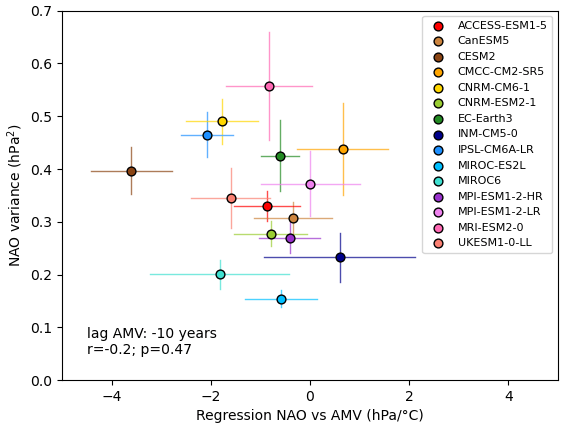
Figure 6 Scatter plot of the ensemble mean 20-year running mean NAO variance (hPa²) versus the regression slope between the 20-year running mean NAO and AMV for DJFM over the 1900–2010 period. The AMV leads the NAO by 10 years.

4.2 Relationship of NAO variability to the Interdecadal Pacific Oscillation

In this section, we explore the possible role of multidecadal variability in Pacific SSTs to explain the spread in multidecadal NAO variability. Indeed, several studies suggest the existence of a teleconnection between low-frequency Pacific SST and North Atlantic atmospheric variability (e.g. Smith et al., 2016; Weisheimer et al., 2017; Seabrook et al., 2023).

There is no significant relationship between the ensemble mean variance of the IPO and the low-frequency NAO variance (Fig. 7a). As for the AMV index, there is also no significant relationship across models between the NAO–IPO regression slope and the low-frequency NAO variance (Fig. 7b). The large-ensemble simulations demonstrate a substantial influence of internal variability on estimating the relationships within single realisations and potentially the observational record, due to the relatively small number of degrees of freedom when considering low-frequency variability (Fig. S4). A positive regression slope between the NAO and IPO is found within the observations, with only a few simulations having a similar magnitude of relationship. As is the case for the AMV, this suggests that a bias is present in the models that could be related to atmosphere–ocean coupling or atmospheric teleconnections. We note that the NAO–IPO relationship at multidecadal timescales has the opposite sign to that at interannual timescales (Fig. S4), as found by Müller et al. (2008), and that the models and observations are in closer agreement at interannual timescales (not shown). This indicates that the bias in NAO connection to the tropical Pacific particularly appears at multidecadal timescales. Seabrook et al. (2023) hypothesised that the opposite sign of the NAO–IPO relationship at multidecadal timescales is related to impacts of the IPO on stratospheric water vapour and subsequent impacts on the polar vortex. If models underestimate the stratospheric water vapour response it may explain the weak amplitude of the relationship. This is a topic for future study.

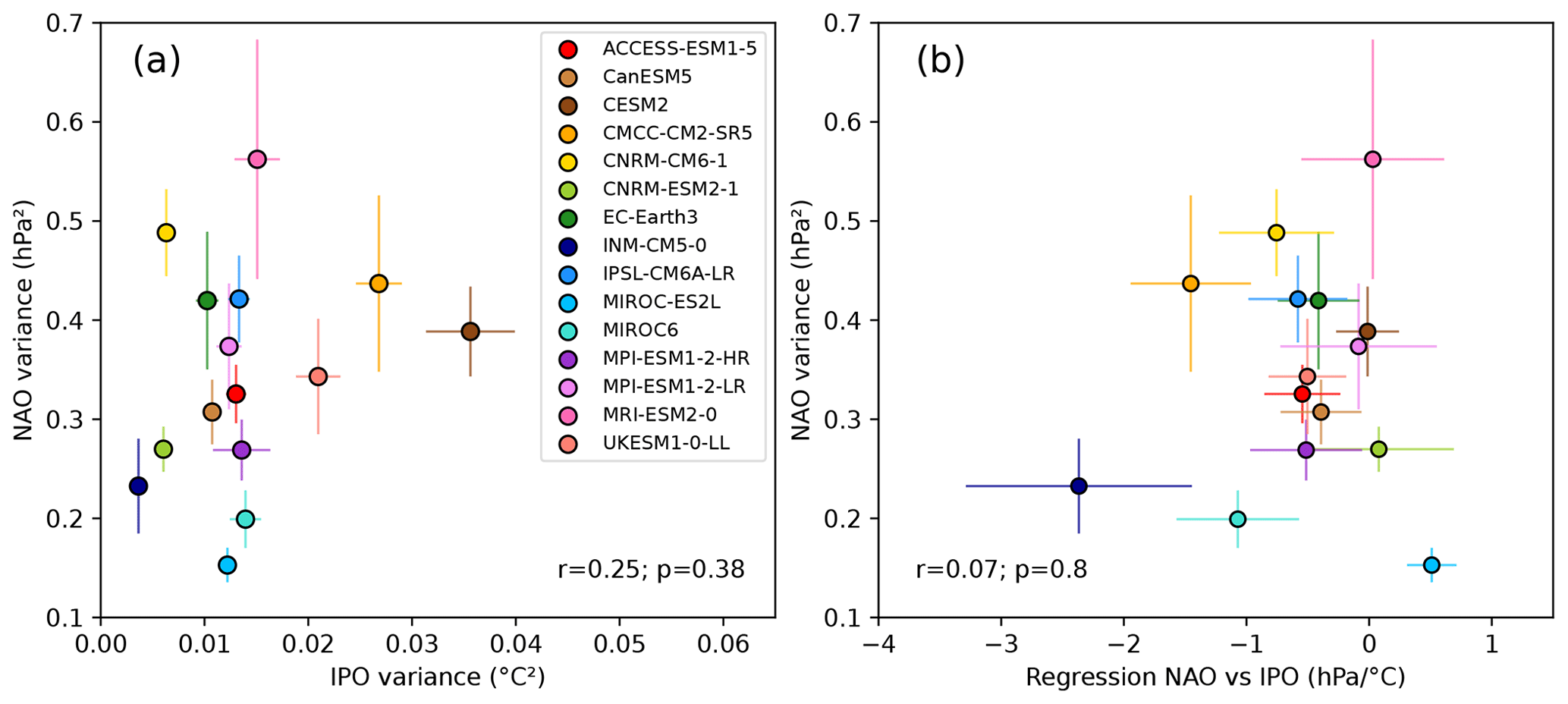
Figure 7 Scatter plot of the ensemble mean low-frequency NAO variance (hPa²) versus (a) the IPO variance (°C²) and (b) the regression slope between the NAO and IPO indices (hPa °C⁻¹) calculated for DJFM over 1900–2010. The variance of the observed IPO is 0.021°C for ERSSTv5.

4.3 Relationship of NAO variability to the stratospheric polar vortex

In this section, we explore the potential role of the polar vortex to explain the spread in low-frequency NAO variability within the CMIP6 models. A causal link between the polar vortex strength and the NAO has been widely demonstrated at sub-seasonal-to-seasonal timescales (e.g. Baldwin et al., 1994; Baldwin and Dunkerton, 2001; Jung and Barkmeijer, 2006; Hitchcock and Simpson, 2014) and at multidecadal timescales (Scaife et al., 2005; Garfinkel et al., 2017; Kretschmer et al., 2018; Butler et al., 2023).

There is a significant positive relationship between low-frequency NAO variability and low-frequency polar vortex variability within the CMIP6 models, with an R²=0.33 (Fig. 8a). We next examine the stratosphere–troposphere coupling strength in the models, estimated as the regression of the low-frequency NAO index onto the polar vortex strength (Fig. 8b; cf. Maycock and Hitchcock, 2015). The stratosphere–troposphere coupling parameter is positive, consistent with the wide literature showing that a stronger vortex is coincident with an anomalously positive NAO index and vice versa (e.g. Charlton and Polvani, 2007). The stratosphere–troposphere coupling parameter at multidecadal timescales is linearly correlated with the parameter estimated using interannual data across models (Fig. S5). This is useful to note because while the satellite record is not yet long enough to constrain stratosphere–troposphere coupling at multidecadal timescales, it is possible to estimate this parameter at interannual timescales (Maycock and Hitchcock, 2015). A significant positive relationship is found between the low-frequency NAO variability and the stratosphere–troposphere coupling (Fig. 8b). A similar result is found using correlations instead of regression coefficients (not shown).

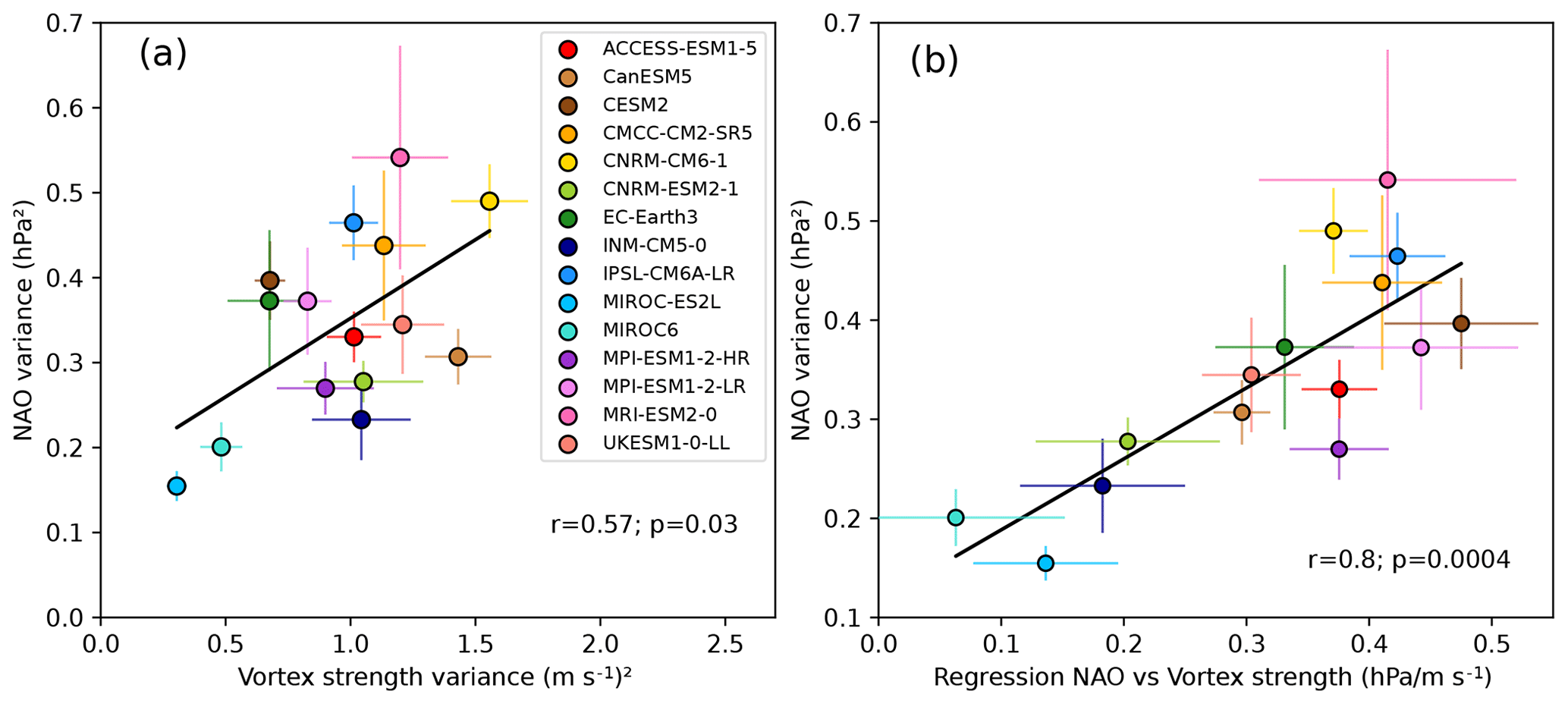
Figure 8 Scatter plot of the ensemble mean low-frequency NAO variance versus (a) the low-frequency polar vortex variance (m s⁻¹)² and (b) the regression slope between polar vortex strength and the NAO (hPa/ms⁻¹) for DJFM over 1900–2010. The black line represents the least-squares regression with the Pearson correlation and p value (see Sect. 2.3).

The vortex variability and stratosphere–troposphere coupling strength are not correlated with one another (r=0.38, p=0.17, Fig. S6), indicating that these are largely independent factors that relate to simulated low-frequency NAO variability. Therefore, both the inter-model spread in the polar vortex strength variance and the inter-model spread in the coupling between the NAO and the polar vortex can explain a large fraction of the spread in the NAO variance at multidecadal timescales. A multilinear regression model including both terms and accounting for their cross-correlation produces a combined R² of 0.72. In any single realisation, there is a large uncertainty in the low-frequency NAO–vortex strength regression slope (Fig. S7), likely due to the relatively low degrees of freedom, indicating the importance of using large ensembles to investigate these multidecadal relationships.

While we cannot isolate causality in these relationships, it has been shown that when a multidecadal stratospheric vortex trend is imposed on a model, the NAO trend is affected (e.g. Scaife et al., 2005). At these timescales, variability in the vortex strength could be affected by external forcing (e.g. solar forcing or volcanoes) or by internally generated unpredictable chaotic variability. While there is a known stratospheric pathway linking tropical Pacific SSTs to the NAO at seasonal timescales (Trascasa-Castro et al., 2019), the lack of relationship between the IPO and low-frequency NAO suggests that the Pacific is not a key driver of modelled NAO spread via a stratospheric pathway at multidecadal timescales.

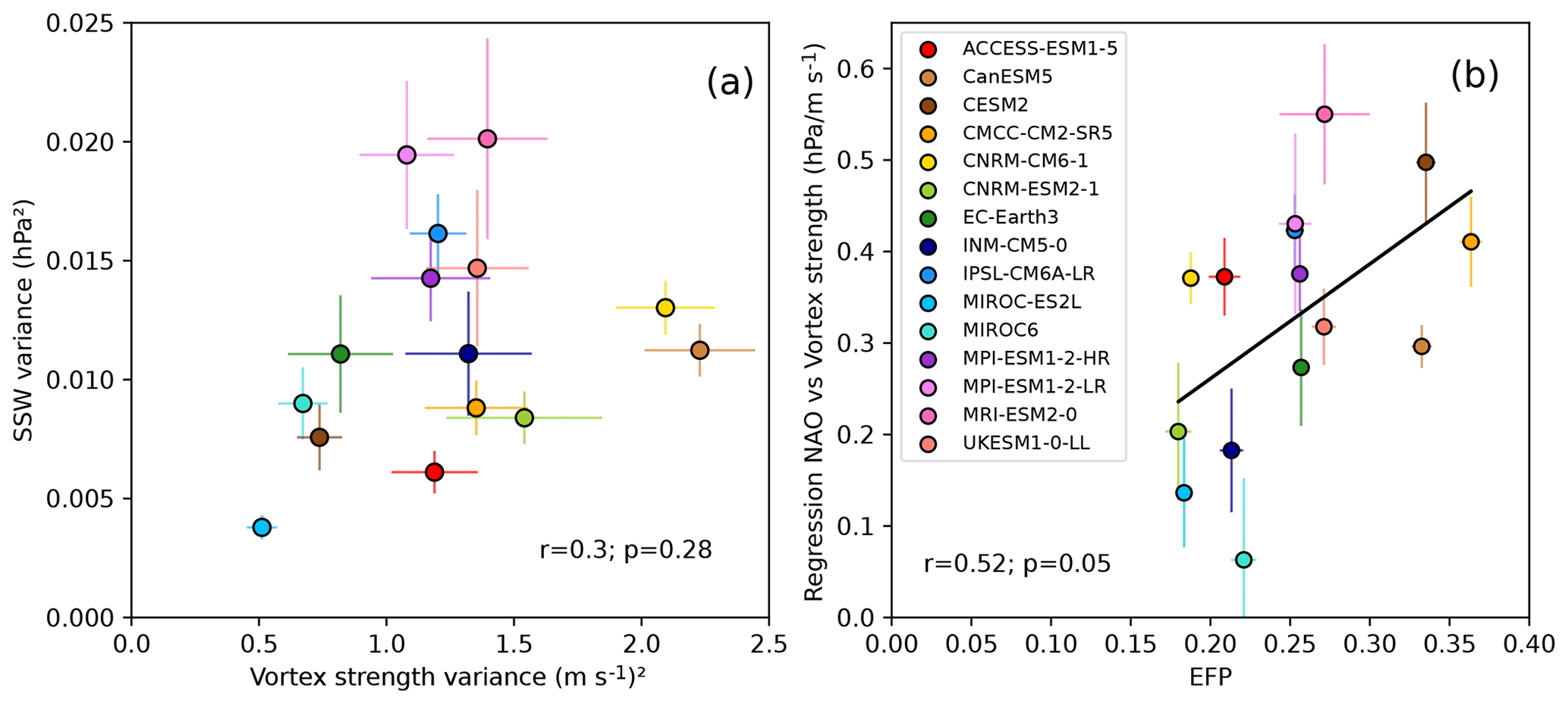
Figure 9 (a) Scatter plot of the ensemble mean 20-year running mean SSW variance (hPa²) versus the polar vortex variance (m s⁻¹)² for DJFM over 1900–2010. (b) Scatter plot of the ensemble mean of the regression slope between the 20-year mean NAO and 20-year mean polar vortex strength (hPa/m s⁻¹) for DJFM over 1900–2010 versus the EFP calculated for each of the ensembles of climate model simulations for the DJFM months over the 1850–2014 period. For the MRI-ESM2-0 and ACCESS-ESM1-5 models, the SSW and EFP periods start in 1950 as they only have daily data available from 1950 onward. The black line represents the least-squares regression with the Pearson correlation and p value (see Sect. 2.3).

5 Possible origins of the spread in polar vortex variability and NAO–polar vortex coupling

The previous section identified a relationship across models between the winter NAO multidecadal variability and the polar vortex variance, as well as with the regression slope between the low-frequency vortex strength and the NAO. This raises questions about the origins of the spread across models in these polar-vortex-related parameters.

One candidate to explain the spread in the low-frequency polar vortex variability is the representation of sudden stratospheric warmings (SSWs). Some studies suggest that models with higher vortex variability also have higher SSW frequency (Hall et al., 2021), whereas other authors have regarded SSWs as the tail of a more normally distributed spectrum of polar vortex variability (Horan and Reichler, 2017). Here, we ask whether the spread in multidecadal vortex variability across CMIP6 models is related to low-frequency variability in the occurrence of SSWs. There is some hint in the reanalysis record of decadal variability in SSW frequency (Domeisen, 2019). Note that daily zonal wind data from MRI-ESM2-0 and ACCESS-ESM1-5 are only available from 1950 onward. No significant relationship is found between the variability in 20-year running mean SSW frequency and the low-frequency polar vortex variability over 1900–2010 (Fig. 9a). The lack of relationship could potentially be related to differences in the amplitude of SSWs in models, and therefore the role of SSWs in driving polar vortex variability would differ. It may also be because low-frequency polar vortex variability is driven by processes unrelated to SSWs, such as low-frequency variability in the upward propagation of planetary wave activity (e.g. Schimanke et al., 2011), or that model biases in subtropical lower stratospheric wind speeds affect the sensitivity of the vortex to upward-propagating waves (Sigmond and Scinocca, 2010), but this is beyond the scope of the current study. However, we note that causality is difficult to establish in this framework as the vortex strength plays a role in setting the conditions for SSWs to occur (Hall et al., 2021; Wu and Reichler, 2020).

We now investigate a potential explanation for the inter-model spread in stratosphere–troposphere coupling strength. Some recent studies have identified a relationship between the amplitude of Northern Hemisphere extratropical circulation responses to external drivers and an estimate of the interaction between eddies and the mean flow (the so-called eddy feedback parameter, EFP; see Sect. 2.2.5). These studies have suggested that models with a weaker EFP exhibit weaker Northern Hemisphere extratropical circulation signals. The tropospheric response to polar vortex variability involves amplification of flow anomalies by eddy feedback (e.g. Song and Robinson, 2004; Domeisen et al., 2013; Hitchcock and Simpson, 2016), so if eddy–mean flow feedback were represented differently in models, this could contribute to spread in the stratosphere–troposphere coupling strength.

We calculate the EFP in the CMIP6 models using the full historical period for all the models (1850–2014) except for MRI-ESM2-0 and ACCESS-ESM1-5, as they only have daily data available from 1950 onward. There is a significant positive relationship between the stratosphere–troposphere coupling parameter and the EFP, with r=0.52 (p=0.05; Fig. 9b). Models with a higher EFP exhibit a stronger stratosphere–troposphere coupling parameter. Conversely, there is no relationship across models between the low-frequency variability in polar vortex strength and the EFP (Fig. S8), suggesting that the tropospheric eddy–mean flow interaction is unrelated to the spread in polar vortex variability. The latter may be more related to the representation of planetary-scale wave forcing, and this would be an area for future study.

6 Discussion and conclusions

In this study, we investigated the representation of multidecadal NAO variability within the CMIP6 historical large-ensemble models and explored statistical relationships with physical factors that could potentially explain inter-model differences in simulated multidecadal NAO variability. When using the full historical simulation (1850–2014) and de-trending by removing the ensemble mean, we find a significant inter-model relationship between the NAO–AMV regression parameter and multidecadal NAO variability ($r=-\mathrm{0.55}$, p<0.05). This suggests that the inter-model spread in multidecadal NAO variability can be partly explained by the representation of AMV–NAO coupling. However, the relationship between AMV–NAO coupling and multidecadal NAO variability across models is quite weak and disappears when using a methodology consistent with that applied in observations (i.e. using a common period with observations and linearly de-trending indices). This overall weak role of the AMV on the NAO may be related to weak atmosphere–ocean coupling in models, as has been suggested in other studies (e.g. Simpson et al., 2018). Indeed, the analysis in Fig. 5b shows that all models analysed fail to capture the lead–lag relationships between the NAO and AMV compared to observations. The amplitude of the NAO–AMV regression slope is too weak in the models, with AMV leading the NAO, and has the opposite sign to observations when the NAO leads the AMV. Consistent with earlier studies (e.g. Kim et al., 2018; Simpson et al., 2018; Bracegirdle, 2022), this points to systematic errors in the modelled representation of atmosphere–ocean coupling in the North Atlantic at multidecadal timescales.

We examine other potential factors that may relate to multidecadal NAO variability and find that the representation of interdecadal Pacific variability does not explain the spread in multidecadal NAO variability, which may arise through tropical–extratropical teleconnections. In contrast, there is a statistically significant relationship across models between multidecadal variability in the stratospheric polar vortex strength and NAO variability (r=0.57, p<0.05). Furthermore, there is a significant relationship across models between the magnitude of a multidecadal stratosphere–troposphere coupling parameter and multidecadal NAO variability (r=0.8, p<0.05), which is largely independent of vortex strength variability. Together these two measures explain around 70 % of the variance in multidecadal NAO variability across models, which is a larger proportion of the inter-model spread than can be explained by the representation of the AMV. While similar relationships have been found in other studies (e.g. Maycock and Hitchcock, 2015), these statistical relationships do not isolate causality. It is possible that the NAO variability itself drives the polar vortex variability or that both factors are related to a common unidentified cause. Nevertheless, there is a wide body of literature demonstrating a causal influence of the polar vortex on the NAO at intraseasonal (Hitchcock and Simpson, 2014), interannual (Ineson and Scaife, 2009; Bell et al., 2009) and decadal timescales (Scaife et al., 2005). Therefore, based on knowledge from the wider literature, we hypothesise that the representation of polar vortex variability and the represented strength of stratosphere–troposphere coupling are both important factors for simulating multidecadal NAO variability. Unfortunately, these parameters cannot be estimated well from observations because the record of stratospheric data is too short to robustly assess multidecadal variability. Nevertheless, the stratosphere–troposphere coupling parameter at multidecadal timescales is correlated with the parameter at interannual timescales in models. The reanalysis record is long enough to estimate the parameters at interannual timescales, so that may offer a route to constraining the model spread.

We find that the inter-model spread in the stratosphere–troposphere coupling parameter is correlated with the relationship between eddy momentum forcing and the zonal mean flow in the extratropical Northern Hemisphere troposphere. On average, a weaker correlation between eddies and zonal mean flow anomalies coincides with a weaker stratosphere–troposphere coupling parameter. This may be indicative of the recognised role of tropospheric eddy feedback in amplifying and maintaining the tropospheric response to stratospheric anomalies (e.g. Song and Robinson, 2004; Domeisen et al., 2013). Weak eddy feedback has been hypothesised as a contributor to the too-weak Arctic Oscillation predictability within climate models at seasonal timescales (Hardiman et al., 2022). The apparent relationship between the stratosphere–troposphere coupling parameter and the eddy–mean flow coupling should be further investigated in controlled experiments.