The role of topography, land and sea surface temperature on quasi-stationary waves in Northern Hemisphere winter: insights from CAM6 simulations

Quasi-stationary waves (QSWs), atmospheric Rossby waves with near constant phase that persist on subseasonal timescales, are not distributed homogeneously across the globe, even at a given latitude. The climatological QSW amplitude has a distinct spatial pattern, with clear zonal asymmetries, particularly in the Northern Hemisphere; those asymmetries must be impacted by stationary forcings such as land, topography, and sea surface temperature (SST). To investigate the effects of stationary forcings on QSW characteristics, including their duration and spatial distribution, eight simulations were conducted using CAM6 with prescribed SSTs. These simulations range from realistic, semi-realistic (with some stationary forcings matching reality) to fully idealized (with idealized forcings added in aquaplanet simulations). The control simulation reproduces the relevant fields well compared to ERA5 reanalysis data. Stationary forcings tend to extend the duration of QSWs and strongly impact their zonal asymmetric distribution. QSWs are primarily influenced by both the local stationary wavenumber Ks, which depends on jet speed and its second-order meridional gradient, and by the strength of transient eddies. However, the covariation between transient eddies and QSWs varies across different types of stationary forcings. In some cases, QSW strength is also associated with the strength of the stationary waves. When the timescale of the QSWs is changed (e.g. from 15–30 to >30 d), the relative contributions from different mechanisms changes, but stationary wavenumber Ks and transient eddy strength are important in all time scales for experiments with realistic land.

1 Introduction

Quasi-stationary waves (QSWs) are extra-tropical Rossby waves with near-constant phase on time scales of several days to weeks and can be closely associated with the occurrence of extreme temperature, precipitation, and wind events (Petoukhov et al., 2013; Kornhuber et al., 2017; Wolf et al., 2018; White et al., 2022; Lin and Yuan, 2022; Li et al., 2024; Chen et al., 2025). Despite their importance as potential precursors to extreme weather events, the mechanisms driving QSWs remain not fully understood. Previous research on the features and mechanisms of atmospheric circulation patterns with similar time scales may help inform our understanding of QSWs, including atmospheric blocking events and planetary scale wave trains or teleconnection patterns (Ali et al., 2022; Teng et al., 2013; Pfahl, 2014; Röthlisberger et al., 2019). In contrast to atmospheric blocking, QSWs have a more longitudinally extended wave-like structure, typically with several consecutive high and low pressure anomalies. The repeated occurrence of QSWs with similar phases over the same region can result in seasonal-averaged patterns, which can be identified as teleconnection patterns (Xu et al., 2019). It is also clear that many features of QSWs, e.g. their frequency, are not uniform across longitudes (Wolf et al., 2018; Fei and White, 2023), as is seen for atmospheric blockings and teleconnections. All these suggest, including topography, a clear role for stationary forcings in shaping the frequency and/or strength of QSWs, including topography (Luo and Chen, 2006; Narinesingh et al., 2020) and diabatic heating (O'Reilly et al., 2016).

We hypothesize that factors influencing the spatial distribution of atmospheric blocking and teleconnections may also influence QSWs. This includes mechanisms such as barotropic instability and non-modal growth, as well as background flow conditions, which can all contribute to blocking and related subseasonal variability (Simmons et al., 1983; Branstator, 1990, 1992; Swanson, 2000, 2002; Nakamura and Huang, 2018). The nonlinear activity of transient eddies interacting with the slowly-varying background flow can play a critical role in the formation of atmospheric blocking directly, particularly in the North Pacific (Hwang et al., 2020). Nakamura and Huang (2018) developed a theory describing the life cycle of atmospheric blocking and provide a framework to quantify the conditions for blocking formation, considering both background flow and Rossby wave activity. The zonal distribution of these background flows, instabilities and transient eddies are ultimately shaped by stationary forcings, including topography and surface temperature gradients (Brayshaw et al., 2009, 2011).

Atmospheric diabatic heating, which is composed of radiation, sensible heating and latent heating, can be a source of Rossby waves. The spatial distribution of diabatic heating is influenced by spatial patterns in surface temperature and related precipitation, particularly convective precipitation. Linear theory explains how diabatic heating in the tropical upper troposphere, primarily stemming from latent heat release during tropical convection, can generate Rossby waves. These waves can propagate away from their source region and may become trapped within midlatitude waveguides (Hoskins and Karoly, 1981; Sardeshmukh and Hoskins, 1988; Hoskins and Ambrizzi, 1993; Jin and Hoskins, 1995; Ding and Wang, 2005; Branstator, 2014). A key example is the Pacific-North America (PNA) pattern, an atmospheric low-frequency mode of variability consisting of a wavetrain extending from the tropical Pacific across North America, which can be driven by diabatic heating sources in the tropics (Franzke et al., 2011). These heating sources may be influenced by tropical internal variability, such as Madden-Julian Oscillation (MJO) and El Niño-Southern Oscillation (ENSO), during which Rossby waves can either propagate through tropical westerlies into the subtropics or reach the subtropics via tropical divergence associated with the diabatic heating (Hoskins and Karoly, 1981; Wallace and Gutzler, 1981; Franzke et al., 2011; Lukens et al., 2017; Wolf et al., 2022). Interestingly, the time scale of the midlatitude Rossby wave response to tropical heating can be much longer than the time scale of the tropical heating (Branstator, 2014). Additionally, anomalous SST patterns in the mid-latitudes, as well as land-ocean temperature contrasts, can serve as heating sources, driving downstream Rossby wave trains (Xu et al., 2019), or modifying the jet waviness (Moon et al., 2022), where the roles of both SST patterns and land-ocean contrast are highlighted. Anomalous soil moisture can also create anomalous diabatic heating and drive the circumglobal teleconnection (Teng and Branstator, 2019).

In addition to diabatic heating, the influence of topography on Rossby waves at subseasonal time scales, particularly related to blockings, has been a focus of research since the last century (e.g. Charney and DeVore, 1979; Charney and Straus, 1980). Charney and DeVore (1979) have shown that topography can induce a quasi-equilibrium state with a relatively weaker zonal component locked close to linear resonance, which is believed to represent atmospheric blocking in highly idealized studies. In more realistic studies, topography has been linked to the phase-locking behavior of QSWs and the weakening of westerlies, which can result in localized summer heatwaves (Jiménez-Esteve et al., 2022). Luo and Chen (2006) suggests that topography helps anchor the locations of atmospheric blocking; however, it has also been found in one model that, while topography may increase the frequency of atmospheric blocking events, it does not necessarily fix their specific locations (Narinesingh et al., 2020).

In addition to the influence on subseasonal variability, potentially including QSWs, as described above, topography and asymmetries in diabatic heating (including land-sea contrast and gradients in SSTs) are the primary drivers of Earth's stationary waves (Garfinkel et al., 2020; White et al., 2021). According to quasi-resonant amplification (QRA) theory, under particular background conditions, stationary waves may be able to resonant with transient eddies to produce high amplitude QSWs (Petoukhov et al., 2013, 2016). Thus topography and diabatic heating sources may have additional influences on QSWs, through their impact on the stationary waves.

The impact of stationary forcings on blockings or subseasonal variabilities, and thus likely on QSWs, does not imply that QSWs cannot exist without such forcings. Indeed, Held (1983) and Wolf et al. (2022) both demonstrate the existence of QSWs in aquaplanet climate model simulations. From a simple perspective of Rossby waves' phase and group speeds, Rossby waves can become (quasi-) stationary if the intrinsic westward propagation of the Rossby waves is countered sufficiently precisely by the eastward advection of the wave by the background zonal winds, resulting in a wave with near-zero phase speed (Hoskins and Ambrizzi, 1993; Hoskins and Woollings, 2015). However, as highlighted by Röthlisberger et al. (2019), the phase speed and group velocity of Rossby waves cannot both be zero simultaneously. This suggests that when Rossby waves become quasi-stationary, i.e., when the phase speed is zero, their group velocity should be positive, resulting in downstream transport of the wave energy. This therefore necessitates a persistent energy source to sustain the QSWs,implying that the presence of QSWs can be the result of multiple factors: a wave source (e.g. tropical convection); suitable propagation conditions (zonal wind); and perhaps also suitable conditions for wave growth (e.g. meridional SST gradients); positive feedbacks between these factors may also be key (Zappa et al., 2011).

Building on previous work that highlights the role of stationary forcings – such as SST patterns and topography – in shaping blockings and other subseasonal variability, we would like to extend this framework to explore their influence on QSWs. While QSWs can emerge even on aquaplanets without stationary forcings, their amplitude, persistence, and spatial distribution are likely modulated by stationary forcings through changes in the background circulation. In this study, we explore how stationary forcing can influence the duration of QSWs and how topography, zonal SST asymmetries and land-ocean contrast can affect QSW distributions in different ways. Specifically, to understand how stationary forcings can influence climatological distribution of QSWs, we test two hypotheses:

1. The spatial distribution of QSWs is associated with and/or modulated by the spatial distribution of stationary waves

2. The spatial distribution of QSWs is modulated by a combination of the stationary wavenumber Ks and the distribution of transient eddy strength/Eady growth rate

To test these hypotheses, we conduct eight climate model experiments that systematically vary stationary forcings. These experiments are described in detail in the Data and Methods section. In the Results, we examine how QSW features – such as amplitude, persistence, and spatial distribution – respond to changes in stationary forcings, with a focus on the Northern Hemisphere winter, where QSWs exhibit their largest amplitude (Wolf et al., 2022). To better elucidate underlying mechanisms, our analysis explores which variables can explain changes in QSWs in response to different stationary forcings, by studying differences between experiment pairs. To confirm the robustness of our conclusions from this analysis, we further use temporal correlations in individual simulations, summarized in the Summary and Discussion section.

2 Data and methods

2.1 Idealized experiments

In this research, we conducted eight 100-year simulations using the Community Atmosphere Model version 6 (CAM6) (Bogenschutz et al., 2018) with prescribed SSTs, with the first 10 years discarded as spin-up period. All experiments with realistic land-ocean distribution used the CESM2 compset F2000climo (atmospheric climatological conditions for the year 2000 with CAM6 physics and finite-volume dynamics core), while aquaplanet simulations used the compset QPC6 (prescribed SST aquaplanet using CAM6), all at a grid spacing of 1.9×2.5°. While the grid spacing is relatively coarse, it is sufficient to capture large-scale circulation patterns, including the QSWs that are the focus of this study. However, the coarse resolution likely results in an inaccurate representation of topography and diabatic heating, affecting their generation, strength, and propagation (Nie et al., 2019; Woollings et al., 2025). ERA5 reanalysis data (Hersbach et al., 2020) is used to compare with a control (CTRL) experiment to confirm that the model captures the main features of observed QSWs. The details of the eight experiments are summarized in Table 1.

Table 1 CAM6 simulations.

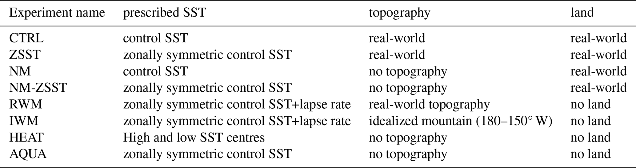
In the CTRL simulation, the full atmosphere and land models are coupled with climatologically prescribed SSTs, including a seasonal cycle. The prescribed SSTs used in the compset F2000climo represents averaged SSTs from the 1995–2005 Hadley Centre Sea Ice and Sea Surface Temperature dataset (HadISST). We perform semi-realistic experiments to isolate the influence of different stationary forcings: in the zonal-SSTs (ZSST) experiment, zonal SST asymmetries are removed; in the no-mountain (NM) experiment, all topography is removed, including the effects of sub-grid scale topography; and in the NM-ZSST experiment, both topography and zonal SST asymmetry are removed. All zonally symmetric SSTs used in our experiments are zonal averages of the observed SSTs, ensuring comparability with the realistic SST experiments. An aquaplanet (AQUA) experiment was also conducted to investigate QSWs without any stationary forcing.

To investigate the importance of land-ocean contrasts and understand stationary forcings in highly idealized situations, we also conducted two “water mountain” experiments based on AQUA. In these experiments, topography was imposed, but without land; a lapse rate of 6.5 K per kilometer was added to the SSTs to avoid anomalous heating sources in the troposphere on top of mountains. Variations of the water mountain experiments – RWM (realistic water mountain) and IWM (idealized water mountain) – were designed to explore the potential impact of topography's shape. The RWM experiment incorporates water mountains that mimic realistic topography. The IWM experiment features a Gaussian mountain spanning 30–60° N and 180–150° W, with a rectangular plateau at 2 km height in the middle, offering an idealized configuration. In the two idealized mountain experiments, the surface geopotential (“PHIS” in CAM6) was calculated based on the AQUA simulation, and only modified in the region of the corresponding added topography. To isolate the impacts of SST anomalies, the HEAT experiment imposed a 20 K positive SST anomaly at 30–60° N, 180–150° W, paired with a 20 K negative SST anomaly at 30–60° N, 150–120° W on the aquaplanet. This zonal temperature contrast in HEAT is designed to replicate the strongest Northern Hemisphere winter surface temperature contrast (Siberia vs. Pacific); while the real contrast is weaker, especially at lower latitudes, we use this strong idealization for a clearer response. We defined the SST anomaly region to span 60 degrees of longitude in the midlatitudes, mimicking the order of magnitude longitudinal extent of an ocean basin or continent.

2.2 Quasi-stationary waves, stationary waves and transient eddies

We calculate quasi-stationary waves strength by assessing the amplitude of persistent Rossby wave packets, using the method outlined by Zimin et al. (2003). The quasi-stationary Rossby wave packet amplitude is calculated from the 15 d Lanczos lowpass filter (Duchon, 1979) applied to the day-of-year anomalous meridional wind at 200 hPa, with only wavenumbers 4–15 included, following Röthlisberger et al. (2019). By using the 200 hPa pressure level, we are studying QSWs slightly higher in the atmosphere than Wolf et al. (2018), who studied QSWs at 300 hPa; we compare the results at different levels and wavenumbers in the Summary and Discussion. The QSW strength is calculated as:

$$\begin{array}{}\text{(1)}& R=\mathrm{|}\mathrm{2}\sum _{k=\mathrm{4}}^{\mathrm{15}}{v}_{\mathrm{tf}}(k,t)e^{\mathrm{2}\mathit{\pi }ik{l}_{\mathit{\lambda }}/N}\mathrm{|}\end{array}$$

where R denotes the strength of quasi-stationary Rossby wave packets, t denotes time, v is meridional wind and v_tf denotes the 15 d lowpass filtered meridional wind. k denotes wavenumber and l_λ denotes the longitudinal grid point index varying from 0 to N, where N is the number of longitudinal grid points.

To study the duration of QSWs, we define QSW events following the methodology outlined in our previous work (Fei and White, 2023), with one modification: the latitude range is adjusted from 35–65 to 30–60° N. This change accounts for the distribution of QSWs in winter in most experiments, which is more concentrated within 30–60° N. In contrast, Röthlisberger et al. (2019) chose 35–65° N because their study focused on summer in realistic world. Quasi-stationary wave events are identified as a series of n consecutive days during which the averaged QSWs amplitude within a region covering 30° of latitude and 60° of longitude exceeds a threshold x. To ensure robustness, we explored two approaches of threshold: fixing either the event frequency or the amplitude threshold x. When the event frequency was fixed at an average of one event per year (90 events in a 90-year run), the amplitude threshold x varied across different experiments. Conversely, when the amplitude threshold was fixed, the number of events increased with stronger stationary forcings, leading to the selection of more and/or longer events.

To maintain a consistent measurement of wave strength, the strength of wavenumbers 4–15 stationary waves and transient eddies were also calculated using Zimin's method, with the 15 d lowpass filtered anomalous meridional wind replaced by the day-of-year climatology for stationary waves and the 15 d Lanczos highpass filtered meridional wind for transient eddies.

2.3 Stationary wavenumber and Eady growth rate

In a barotropic framework, the stationary wavenumber Ks, calculated from the background flow conditions, describes the maximum wavenumber of a Rossby wave that can become stationary (Hoskins and Ambrizzi, 1993), i.e. ${\mathrm{Ks}}^{\mathrm{2}}=k^{\mathrm{2}}+l^{\mathrm{2}}$ for a stationary wave, where k and l are the zonal and meridional wavenumbers respectively. In Mercator projection, the stationary wavenumber can be written as an equivalent zonal wavenumber (Hoskins and Ambrizzi, 1993). We analyse the impact of changing stationary wavenumbers on the distribution of QSWs in our different experiments, so the Ks is defined at 200 hPa, the same as QSWs strength. We calculated the climatology of stationary wavenumber Ks across all experiments using daily zonal wind data filtered with a 15 d low-pass filter to reduce the non-linear impacts of high frequency waves, based on the following definition:

$$\begin{array}{}\text{(2)}& {\displaystyle }\mathrm{Ks}=a\sqrt{{\displaystyle \frac{{\mathit{\beta }}_{\mathrm{m}}}{U_{\mathrm{m}}}}}\text{(3)}& {\displaystyle }{\mathit{\beta }}_{\mathrm{m}}={\displaystyle \frac{\mathrm{2}\mathrm{\Omega }{\cos }^{\mathrm{2}}\mathit{\varphi }}{a}}-{\displaystyle \frac{\cos \mathit{\varphi }}{a^{\mathrm{2}}}}{\displaystyle \frac{\partial }{\partial \mathit{\varphi }}}{\displaystyle \frac{\mathrm{1}}{\cos \mathit{\varphi }}}{\displaystyle \frac{\partial }{\partial \mathit{\varphi }}}\left(U_{\mathrm{m}}{\cos }^{\mathrm{2}}\mathit{\varphi }\right)\end{array}$$

where a denotes the radius of the Earth, ϕ denotes the latitude, β_m is the meridional gradient of absolute vorticity in Mercator projection, and U_m is the zonal wind in Mercator projection.

To study the potential for the growth of waves, we use the Eady growth rate, derived from the Eady Model (Eady, 1949), which effectively represents local baroclinic instability. It can be defined using zonal wind or temperature by an approximation form of thermal wind balance and we further use hydrostatic balance and ideal gas law to approximate the Brunt-Väisälä frequency N. Here, we adopt the following definition (Lindzen and Farrell, 1980):

$$\begin{array}{}\text{(4)}& {\displaystyle }{\mathit{\sigma }}_{\mathrm{E}}=-\mathrm{0.31}*{\displaystyle \frac{g}{NT}}{\displaystyle \frac{\partial T}{\partial y}}\text{(5)}& {\displaystyle }N=\sqrt{{\displaystyle \frac{g}{\mathit{\theta }}}{\displaystyle \frac{\partial \mathit{\theta }}{\partial z}}}=\sqrt{-{\displaystyle \frac{g^{\mathrm{2}}p}{RT\mathit{\theta }}}{\displaystyle \frac{\partial \mathit{\theta }}{\partial p}}}\end{array}$$

where σ_E denotes Eady growth rate, g denotes the acceleration due to gravity, N is the Brunt-Väisälä frequency, T represents the temperature, y is the northward distance, z represents the vertical coordinate, p represent the pressure coordinate, and R is the gas constant for dry air. We choose the Eady growth rate at 700 hPa in our analysis because it represents a low level where baroclinic instability is strong in most situations (e.g., Simmonds and Lim, 2009).

3 Results

3.1 The duration of quasi-stationary wave events

We first explore the duration/frequency of discrete QSW events in the different experiments. We focus on the North America region (Fig. 1), but conclusions for a region over Europe (see Fig. A1) are very similar. When the amplitude threshold of events is fixed, the CTRL CAM simulation tends to over-simulate the frequency of short events relative to ERA5, and under-simulate the frequency of long events (Fig. 1). This bias, of too many short events, and too few long events, can also be seen in the bottom row of Fig. 1, where the black dashed line shows the ERA5-CTRL difference, highlighting a potential bias in CAM6's representation of QSW persistence. This bias is consistent when selecting QSW events with a fixed frequency threshold, i.e. changing the threshold to select the same number of events in each experiment(Fig. A2) and in different regions (Fig. A1).

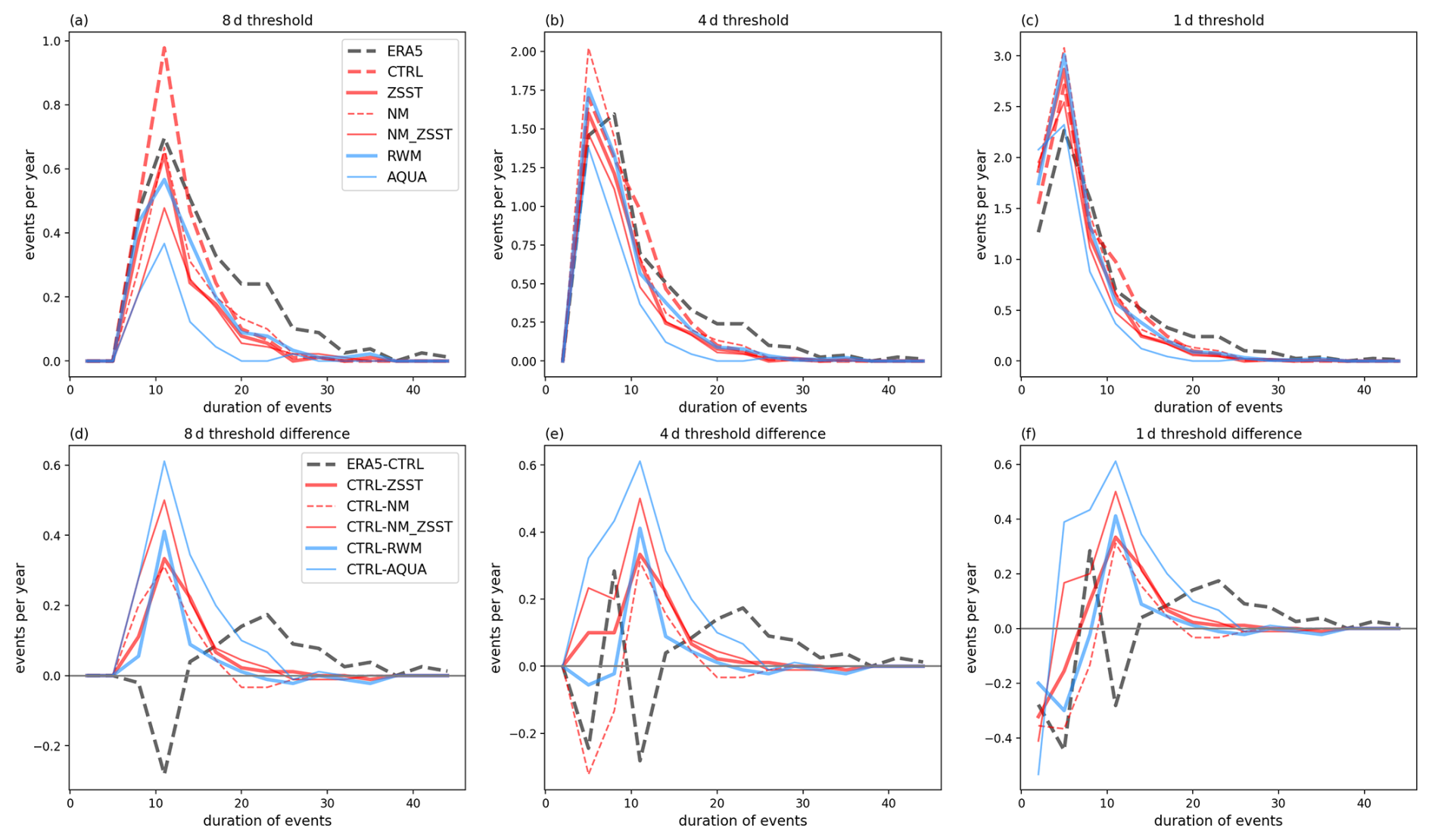
Figure 1 The duration-frequency distribution of QSW events across different experiments within the “North America” region, defined as the area between 60 and 120° W. The first row shows distributions for thresholds of (a) 8, (b) 4, and (c) 1 d on the QSW metric. The second row shows ERA5-CTRL, as well as the difference between the CTRL and other experiments (as CTRL – experiment) for thresholds of (d) 8, (e) 4, and (f) 1 d. Events are all selected using a fixed amplitude threshold. The lines are smoothed with 3 d bins on the x-axis. The color coding is as follows: ERA5 is shown in black, experiments with realistic land-ocean contrast are in red, experiments without land surfaces in blue. Dashed lines represent experiments with zonally asymmetric SSTs, while solid lines indicate those with zonally symmetric SSTs. Thick lines correspond to experiments that include topography, whereas thin lines represent experiments without topography.

Figure 1 also illustrates the QSW duration distributions with fixed amplitude between the CTRL experiment and other experiments with the bottom row showing the differences between experiment pairs to show the role of stationary forcings on QSW durations more clearly. Regardless of the applied duration threshold (different columns), adding stationary forcings consistently increases the frequency of QSWs with durations peaking around 12 d, while slightly decreasing the frequency of QSWs with shorter durations (Fig. 1). Note that here, duration refers to the number of consecutive days when the QSW amplitude exceeds the threshold; the 15 d low pass filter in the QSW definition still requires persistence on this timescale, even for a 1 d event. The disproportionately higher increase in longer events relative to the decrease in shorter QSW events illustrates an overall increase in the absolute number of events as well when adding stationary forcings. This highlights the critical role of stationary forcings in either generating more frequent or stronger QSWs (as evident in Fig. 1d, where the frequency of QSWs almost universally increases) or sustaining QSWs for longer durations (indicated by the reduction in frequency of events shorter than 10 d and increase for those exceeding 10 d in some experiment pairs, e.g. CTRL-NM and CTRL-RWM in Fig. 1e and f), or both. The underestimation of long-lasting events and overestimation of shorter events in ERA5 relative to CTRL may be partially attributable to the reduced stationary forcings from the prescribed SSTs, as without coupling systems and interannual variations in SSTs, some forcings are omitted from the model. Alternative regional definitions yield similar results (Fig. A1), indicating the robustness of the analysis.

3.2 The spatial distribution of quasi-stationary waves

We now investigate the spatial distribution of QSWs, and the effects of stationary forcings on this distribution. Based on previous theories of teleconnections and blocking, we test the two hypotheses introduced at the beginning of this study:

• Hypothesis 1. The spatial distribution of QSWs is associated with the spatial distribution of stationary waves, due to a similar influence of stationary forcings on both stationary and quasi-stationary waves, e.g. through zonal wind changes, or due to wave resonance between stationary waves and transient eddies resulting in QSWs.

• Hypothesis 2. The spatial distribution of QSWs is modulated by a combination of stationary wavenumber (Ks) and transient eddy strength/local Eady growth rate, as Rossby waves with given wavenumbers can become stationary under background conditions with the corresponding stationary wavenumbers.

To test these hypotheses, four variables – stationary wave strength, stationary wavenumber (Ks), transient eddy strength, and Eady growth rate – are analyzed. We analyse “stationary wave strength” to assess the first hypothesis. Conversely, analysis of correlations between QSWs and the “stationary wavenumber Ks” and “transient eddy strength” relate to the second hypothesis, along with “Eady growth rate”, as high values of Eady growth rate indicate regions where Rossby waves may grow rapidly. The potential of Rossby wave growth may be important as Hypothesis 2 applies regardless of whether strong Rossby waves propagate into the region (as transient eddies) or are generated locally. Thus, Eady growth rate helps assess whether local instability contributes to explaining the spatial distribution of QSWs. Whether different stationary forcings affect the circulation patterns – and thus the QSWs differently – will be discussed throughout the analysis.

Before analyzing the differences across experiment groups, we first evaluate whether our CTRL simulation effectively replicates the observed spatial distribution of QSWs, and the four metrics of interest (Fig. 2). Overall, the zonal and meridional wind climatologies are well-represented in CTRL (compare Fig. 2a and b). The QSWs strength (shown in the coloured shading in Fig. 2c–h), is also generally well represented, although with an under-simulation of climatological QSW strength over Europe and the Atlantic. For stationary wavenumber Ks (black contours in Fig. 2c and d), the regions where $\mathrm{4}\leqq \mathrm{Ks}\leqq \mathrm{8}$ are again generally well represented, although the CTRL simulation underestimates the value of Ks at many high-latitude regions. We focus on regions where $\mathrm{4}\leqq \mathrm{Ks}\leqq \mathrm{8}$ due to the high correspondence of this range with regions of strong climatological QSW strength, as can be seen in both ERA5 (Fig. 2c) and CTRL (Fig. 2d). In Fig. 2e and f, we see that the transient eddy strength is underestimated in CTRL, particularly over land, although the spatial pattern is well simulated. Similarly, the spatial distribution of the Eady growth rate, including the peaks over the western Pacific and Atlantic are captured (Fig. 2g and h). To quantify the similarities, the spatial correlations of these variables between ERA5 and CTRL are all above 0.9 (see the top-right corners of the subplots in the left column). Spatial distributions of climatological QSWs strength, zonal and meridional wind, stationary wavenumber Ks 4–8 range and transient eddy strength in all other experiments can be found in the Appendix, in Figs. A3, A4, A5 and A6 accordingly.

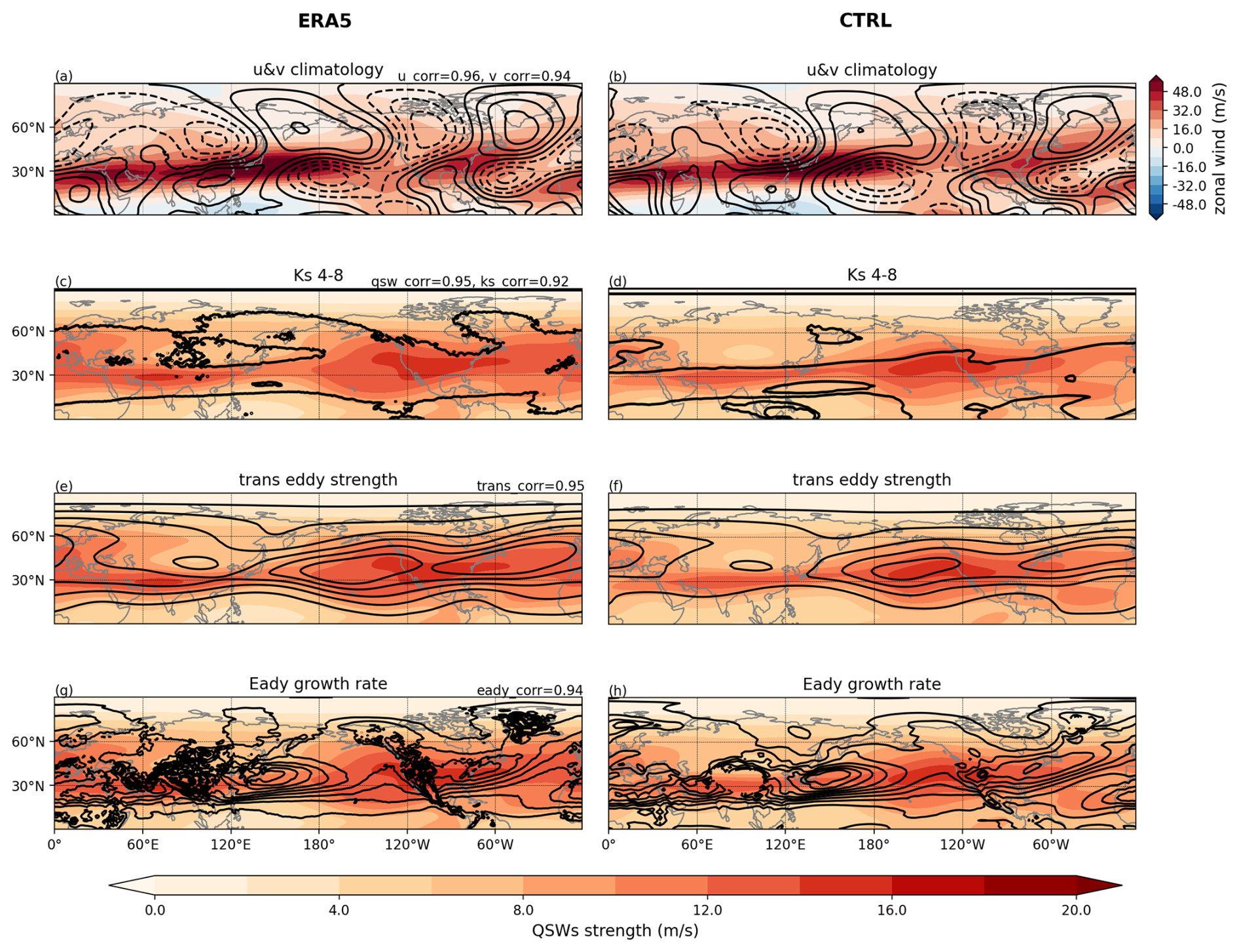
Figure 2 Climatologies for DJF in ERA5 (left column) and the CTRL simulation (right column). Panels (a) and (b) depict the zonal wind climatology (shading) and meridional wind climatology (contours) with different colorbar. The contour interval is 3 m s⁻¹. In subsequent plots, shading consistently represents QSW strength. Contours in (c) and (d) show the stationary wavenumber Ks range where $\mathrm{4}<=\mathrm{Ks}<=\mathrm{8}$ (e) and (f) show transient eddy strength with 2 m s⁻¹ contour interval, (g) and (h) display the Eady growth rate at 700 hPa with 0.1 per day contour interval. The Eady growth rate in CTRL is masked over regions where topography exceeds 1500 m. The values in the top right of the panels in the left column show the correlation coefficients between ERA5 and CTRL.

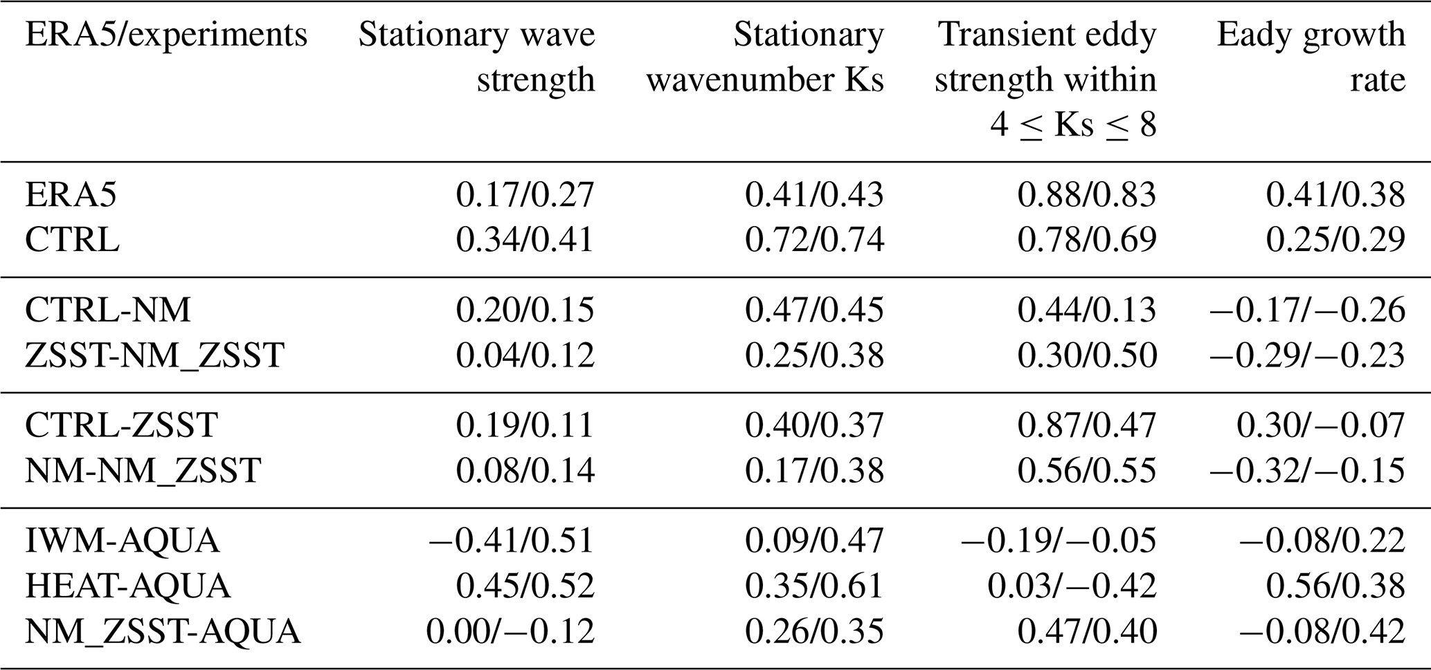
To assess whether our hypotheses are consistent with observed distributions, we first calculate Spearman’s rank correlation coefficients across the Northern Hemisphere mid-latitudes (15–75° N) between climatological values of each of these metrics and the climatological QSW strength. These values, for ERA5 and the CTRL simulation, are shown in the upper section of Table 2. The spatial distribution of QSWs in both ERA5 and CTRL shows relatively strong positive correlations with all metrics. While spatial correlation is a limited method for measuring complex associations between QSWs and other metrics, the positive correlations suggest that multiple mechanisms may affect the QSW spatial distribution. As more stationary forcings are introduced, altering these metrics, their interactions may make it increasingly challenging to isolate and understand the impacts of these stationary forcing on QSWs.

Table 2 The spatial correlations between QSW strength and different metrics in ERA5 and experiments calculated between 15–75° N for DJF. The values in brackets indicate the variation in correlation coefficients when selecting either the first or last 45 years as an estimate for uncertainty. The simulations are separated by sections, with ERA5 and CTRL at the top, then the impact of realistic topography (CTRL-NM and ZSST-NM_ZSST), then the impact of realistic zonal SST gradients (CTRL-ZSST and NM-NM_ZSST), and in the bottom section, highly idealized simulations including the impact of land (NM_ZSST-AQUA). The bold correlation coefficients are significant at 95 % level.

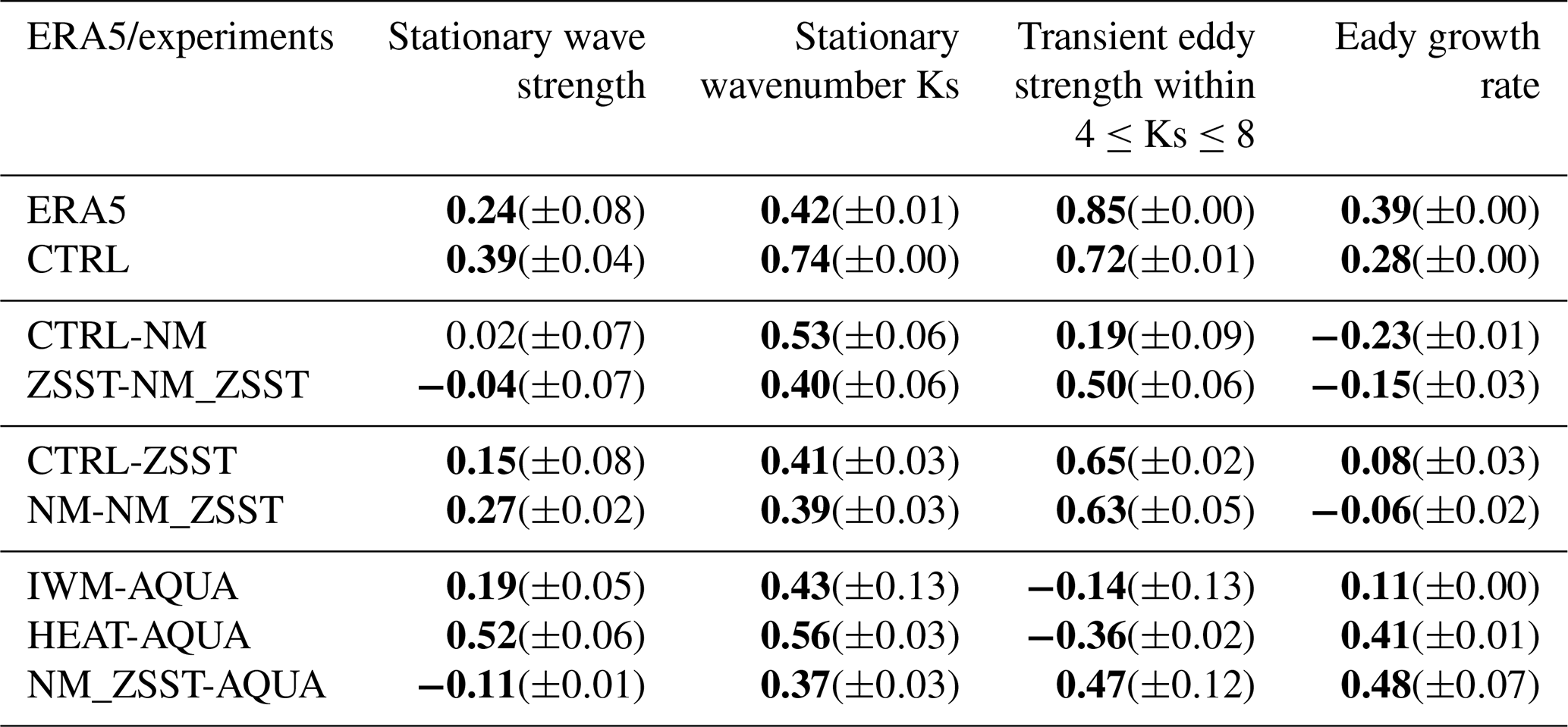
Thus, to isolate each stationary forcing in turn, and analyse the impacts on the QSWs, the lower section of Table 2 presents correlation coefficients for climatological differences in each metric with climatological differences in QSW strength across different experiment pairs, highlighting the impacts of topography, zonal SST asymmetry, and land surface on QSWs strength changes. We aim to better understand what stationary forcings affect QSWs, and the underlying mechanisms, which will be discussed more in Sect. 3.2.1 to 3.2.3.

To assess the role of internal variability on the correlation coefficients, we separate the 90 years of data into two 45-year periods – the correlation coefficients in Table 2 do not show significant variation across these different time periods (numbers in parentheses give the variability across the two 45-year periods). In addition, we use more than one pair of experiments to study the impacts of topography and zonal SST gradients, as shown in the sections in Table 2. For example, we use both CTRL-NM and ZSST-NM_ZSST to understand the role of topography, and find strong similarities in the correlation coefficients between these matching pairs, giving further confidence in the robustness of these results.

3.2.1 Hypothesis 1: association with stationary waves

To test the first hypothesis, we focus on stationary waves with the wavenumber 4–15 range to match the wavenumber range of the QSWs. We study differences in the strength of these stationary waves between different experiment pairs, and compare to differences in QSW strength (Fig. 3). Notably, in most of the experiment comparisons, there is little association between regions where stationary waves are strengthened, as indicated by solid contours, and regions where QSWs are strengthened, as indicated by red shading. Similarly, weakened stationary waves indicated by dashed contours and weakened QSWs indicated by blue shading rarely appear in the same locations. This is further illustrated by generally weak (although often positive, particularly in response to SST gradients) spatial correlation coefficients, given in the top right corner of each panel (and summarized in Table 2), suggesting a weak connection between changes in the stationary waves and the changes in the QSWs; the exception to this is HEAT-AQUA, with a correlation of 0.52 (Fig. 3f). Larger positive correlations in response to SST gradients (Fig. 3b, d, f) than to topographic changes (Fig. 3a, c, e) suggest a potential link between stationary wave strength and QSW strength. However, generally weak correlations imply that this relationship does not primarily explain changes in QSW spatial distribution under highly idealized experiments like HEAT-AQUA.

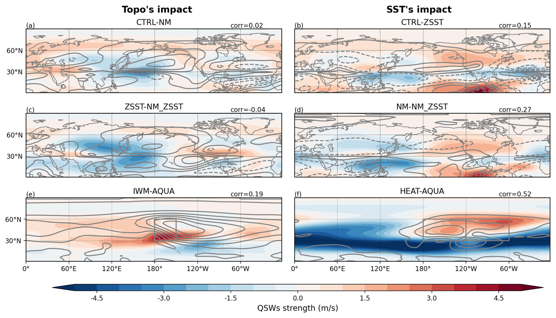
Figure 3 Climatological quasi-stationary wave strength (shading) and and wavenumber 4–15 stationary wave strength (contours), with their Spearman's rank correlation coefficients over 15–75° N attached at top-right corners of subplots. Subplots (a) and (c) display differences between the CTRL and NM, and between ZSST and NM-ZSST. Subplots (b) and (d) show the differences between CTRL and ZSST, and NM and NM-ZSST. Subplots (e) and (f) present differences between IWM and AQUA, and HEAT and AQUA. The left column shows differences illustrating the impact of topography, whilst the right column illustrates the impacts of SST gradients. The contour interval is 1 m s⁻¹.

While the observed positive correlations between stationary waves and QSWs (Table 2) are consistent with the possibility of wave resonance as a mechanism for high amplitude QSWs, it is also possible that the positive correlations are caused by the same factors that influence stationary waves having a similar effect on QSWs, and not a direct causal relationship between stationary wave strength and QSW strength. For example, QSWs may be linked to zonal wind in different ways in our hypotheses, and stationary wave strength can also be influenced by zonal wind. Specifically, mechanical forcing from topography interacts with zonal wind, and the strength of stationary waves can vary with the incoming speed and angle of zonal wind as response.

3.2.2 Hypothesis 2: stationary wavenumber Ks makes Rossby waves quasi-stationary

We now explore Hypothesis 2, starting with the association between QSWs and the stationary wavenumber Ks. The highest values of climatological QSW amplitude are typically found where the climatological stationary wavenumber is between 4–8, across a range of very different experiments (Fig. 4). In the AQUA experiment, the relationship between Ks and QSW strength is very clear, with little variability (Fig. 4), and QSW strength peaks within $\mathrm{5}\le \mathrm{Ks}\le \mathrm{7}$. As more stationary forcings are introduced – such as a single Gaussian water mountain in IWM (Fig. 4c), realistic water mountains in RWM (Fig. 4b), and ultimately in the CTRL (Fig. 4a) experiment – the relationship observed in AQUA becomes increasingly diffuse. However, the “best Ks range” for large QSWs amplitude remains between $\mathrm{4}\le \mathrm{Ks}\le \mathrm{8}$.

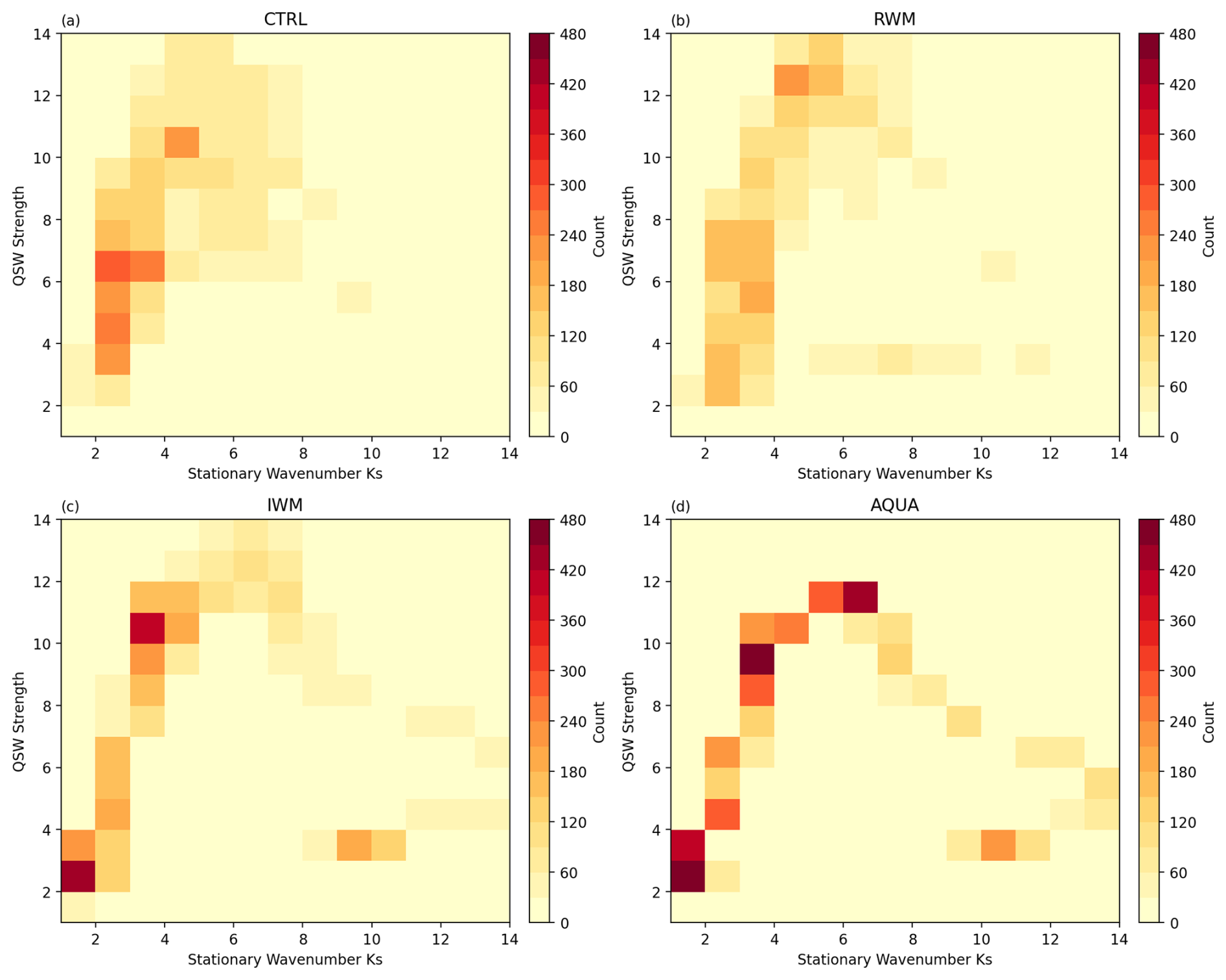
Figure 4 Heatmap showing the number of grid points in winter (DJF) climatology that stationary wavenumber Ks is x with a QSW strength of y in Northern Hemisphere. (a) shows the statistics in CTRL, (b) for RWM, (c) for IWM and (d) for AQUA.

An interesting question arises from Fig. 4: what causes the distinct shape of the heatmaps in Fig. 4, particularly for the AQUA simulation (Fig. 4d)? Since this distinct shape remains relatively consistent regardless of stationary forcings, although more diffuse as more forcings are introduced, it may not be directly related to our main research question of how stationary forcings affect QSWs features; however, understanding this distribution may help understand the underlying mechanisms of QSWs. One potential explanation is a dependence on latitude. Both QSW strength and Ks have a similarly clear relationship with latitude, which is more distinct in AQUA and becomes more diffuse, but still recognizable, as more stationary forcings are added (see Figs. A7 and A8). This suggests that the beta effect in the stationary wavenumber Ks metric, which has a direct dependence on latitude, plays an important role in the total Ks, particularly in idealized simulations such as AQUA. With stronger stationary forcings, the background circulation undergoes greater modification, weakening the relationship between latitude and Ks and also between latitude and QSW strength. The observed “diffusion” of this relationship when additional stationary forcings are introduced highlights that factors beyond latitude – such as stationary forcings – also influence QSWs distribution, emphasizing the relevance of our research question. In these idealized experiments, as stationary forcings are removed, from Fig. A7a to d, the latitude range where $\mathrm{4}\le \mathrm{Ks}\le \mathrm{8}$ shifts equatorward from 20–50 to 15–35° N; a corresponding equatorward shift in the QSW strength peak, which moves from 30–40 to 20–30° N (Fig. A8a to d), suggests a connection between Ks and QSW strength. To further confirm the relationship between QSW strength and Ks, we show the stationary wavenumber Ks distribution overlaid on the climatological QSW distribution in the maps in Fig. A5. In Fig. A5j (AQUA), the darkest shading aligns precisely with the wavenumber range of 4–8.

We further assess the effectiveness of this stationary wavenumber hypothesis, specifically that QSWs are most likely in regions where $\mathrm{4}\le \mathrm{Ks}\le \mathrm{8}$, by studying the changes under different stationary forcings. While we do not expect a precise match between Ks of particular values and QSW strength, as QSWs can have a range of both zonal and meridional wavenumbers, we use a proxy for how close the stationary wavenumber is to values between 4 and 8: the absolute difference between the local Ks and a value of 6. Thus, locations with a climatological value of Ks of 5, or 7, would have a value of 1; locations with a Ks value of 3 or 9 would have a value of 3. We then analyze the differences in $|\mathrm{Ks}-\mathrm{6}|$ and QSW strength across experiments (Fig. 5). If our hypothesis – that smaller values of $|\mathrm{Ks}-\mathrm{6}|$ typically correspond to stronger QSWs – is correct, a decrease of $|\mathrm{Ks}-\mathrm{6}|$ (e.g., in CTRL compared to NM) should coincide with an increase of QSW strength, as the stationary wavenumber moves closer to 6. To simplify interpretation, we multiply the change of $|\mathrm{Ks}-\mathrm{6}|$ by −1, such that, if our hypothesis is correct, then regions where Ks approaches 6 (now shown as positive contours) will align with areas of higher QSW amplitude (positive shading), and the correlation coefficients between Ks and QSW strength will be positive. QSW strength will not peak at a stationary wavenumber of 6 precisely across all regions and experiments, rendering this analysis somewhat qualitative. To ensure the robustness of the stationary wavenumber hypothesis in explaining QSW distributions, we also examined patterns for choosing stationary wavenumber values of 5 and 7, i.e. calculating differences in $|\mathrm{Ks}-\mathrm{5}|$ or $|\mathrm{Ks}-\mathrm{7}|$, finding minimal variations in the conclusions.

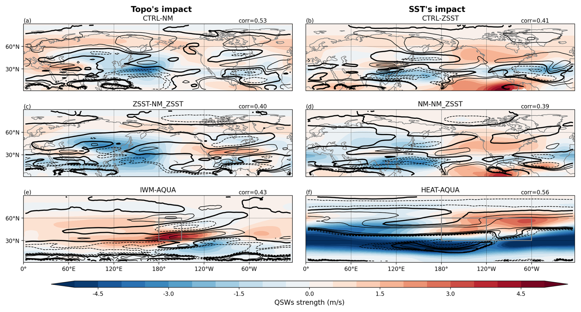
Figure 5 How much the stationary wavenumber Ks deviate from Ks=6 ($|\mathrm{Ks}-\mathrm{6}|$) multiplied by −1 (black contours) and QSW strength (shading). The contour interval is 0.5 m s⁻¹ and contour lines are centered smoothed every 3 grid points. Other information is the same as Fig. 3.

For all experiment pairs, regions where Ks becomes closer to 6 tend to have an increased QSW strength (Fig. 5), resulting in relatively high positive correlations (Fig. 5 and Table 1). One consistent exception to this is downstream of Asian topography in CTRL-NM (Fig. 5a) and ZSST-NM_ZSST (Fig. 5c), where there are regions of Ks closer to 6 (positive black contours), but decreased climatological QSW amplitude (blue shading). However, over the hemisphere, there are strong positive correlation coefficients in all experiment pairs studying the impacts of topography (0.40 to 0.53). The correlation coefficients in experiment pairs reflecting changes in zonal SST patterns are within a similar range (0.39 to 0.56, right column), suggesting that in most regions, both topography and zonal SST asymmetry may modulate QSWs through their influence on local stationary wavenumber. The Ks hypothesis, that high amplitude QSWs are more likely when Ks is closer to 6, is also supported by results from stationary forcings like land-ocean heat contrast and/or land surfaces friction, shown in Fig. A9c.

The analysis above confirms that where the climatological stationary wavenumber Ks gets closer to a value of 6, climatological QSW strength tends to increase. We now explore the role of transient eddy strength, as it is also crucial for this hypothesis: under appropriate background flow conditions, transient eddies can decelerate and become quasi-stationary; if there are no transient eddies, the favorable background condition cannot produce QSWs. Alternatively, if there is a higher Eady growth rate, suggesting transient eddies can grow more easily at a particular location, we may expect more QSWs to form at that location without large transient eddy strength upstream.

Based on our hypothesis, changes in transient eddies will only have an influence on QSWs if they are within, or close to, a region of $\mathrm{4}\le \mathrm{Ks}\le \mathrm{8}$. Thus we focus on studying the changes in transient eddies within regions of $\mathrm{4}\le \mathrm{Ks}\le \mathrm{8}$. In experiments where realistic land is included, most changes in the strength of transient eddies are highly correlated with changes in QSW strength within the $\mathrm{4}\le \mathrm{Ks}\le \mathrm{8}$ range (Fig. 6a–d, values on the left), suggesting an association between transient eddies and QSW strength. However, outside of the region where $\mathrm{4}\le \mathrm{Ks}\le \mathrm{8}$ (values on the right), the correlations between changes in transient eddy strength and changes in QSW strength are weaker, or negative (Fig. 6a). This is because when background conditions conducive to QSWs ($\mathrm{4}\le \mathrm{Ks}\le \mathrm{8}$) can not be fulfilled, the transition of transient eddies to QSWs is inherently limited. Even though transient eddy strength is suppressed in the surrounding regions of topography (Brayshaw et al., 2009), these changes cannot have much impact on the climatological QSWs. However, although the correlation in Fig. 6c is relatively high (0.50), the low correlation coefficients in the left column of Fig. 6a and e suggest a secondary – or even negative – impact of transient eddies on QSW strength. This highlights that the role of transient eddies can vary across different model configurations when considering the impact of topography on QSWs.

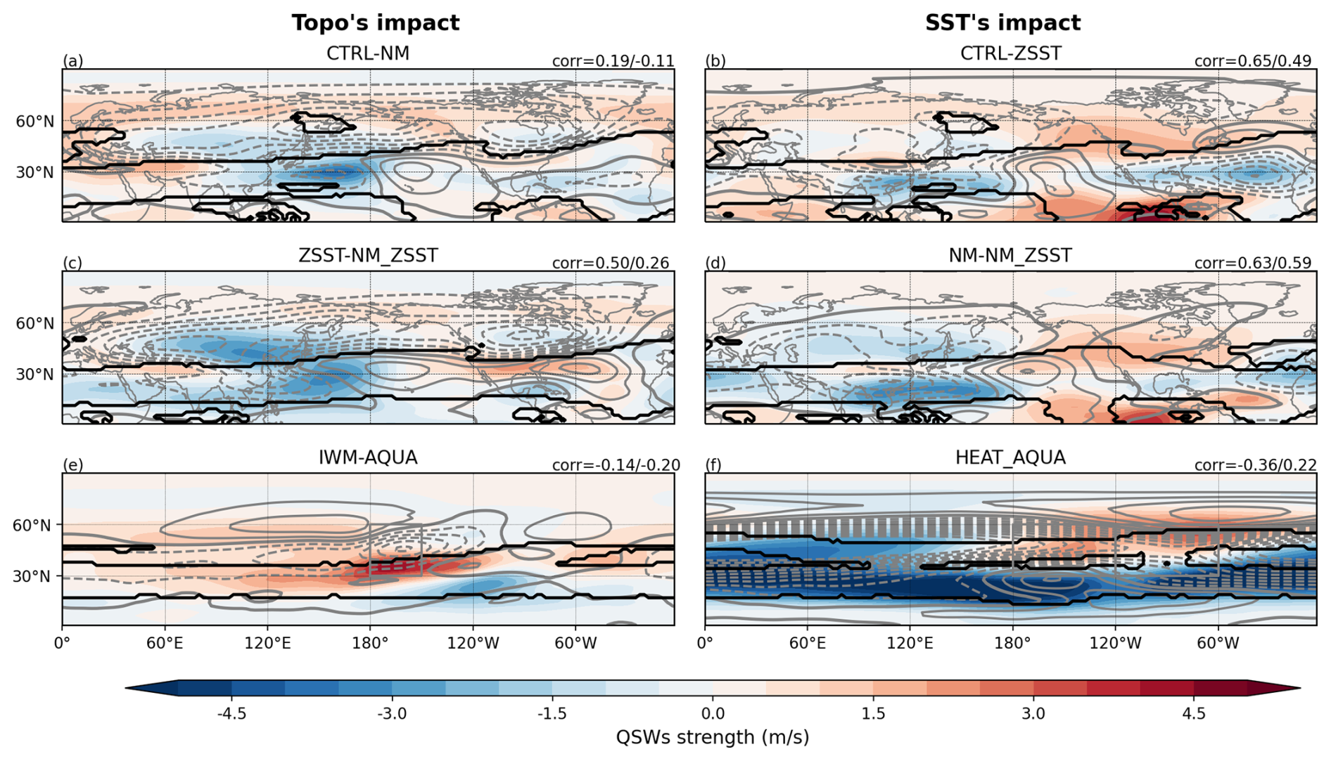
Figure 6 The same as Fig. 3, except gray contours show transient eddy strength and black contours show stationary wavenumber $\mathrm{4}\le \mathrm{Ks}\le \mathrm{8}$. The left correlation coefficients are calculated between QSW strength changes and transient eddy strength changes within $\mathrm{4}\le \mathrm{Ks}\le \mathrm{8}$, while the right correlation coefficients are calculated over all grid boxes between 15–75° N.

For experiment pairs studying the impact of SST gradients (right column in Fig. 6), the correlation between transient eddy changes and QSW strength changes is higher in the experiments showing the impact of realistic zonal SST asymmetry i.e. Fig. 6b and d, in which QSWs and transient eddies tend to be weakened and strengthened in the same regions. In HEAT-AQUA, the correlation drops from positive to strongly negative when focusing on the $\mathrm{Ks}=\mathrm{4}-\mathrm{8}$ range in the Northern Hemisphere; this is likely because of the large change in Ks between these two experiments (see Fig. 5f), particularly equatorward of 40° N where Ks shifts substantially away from a value of 6.

Notably, our hypothesis suggests a trade-off between QSWs and transient eddies: QSWs are generated when transient eddies become stationary, which may in turn reduce the amplitude of transient eddies in regions that become more favorable for QSW formation. Conversely, in regions where the background conditions are already favourable, an increase in transient eddies could lead to an increase in QSWs. The relationship between changes in transient eddy strength and changes in QSW strength is therefore complex, and the positive correlations found in SST's impact experiment pairs suggests that stationary forcing influence on transient eddies dominates over the conversion of transient eddies into QSWs, and vice versa. In IWM-AQUA and HEAT-AQUA, however, the appearance of a region of $\mathrm{4}\le \mathrm{Ks}\le \mathrm{8}$ (see Fig. 6e and f thick black contours) may be responsible for both the increase in QSWs (see Fig. 6e and f shading) and the decrease in transient eddies (see Fig. 6e and f contours), as transient eddies become more quasi-stationary. This may explain the negative correlations between transient eddy changes and QSW changes found for these experiment pairs. In experiment pairs reflecting the impact of topography, the relationship between transient eddies and QSWs may be more complex due to the overall reduction in transient eddy activity when topography is included. We analyze the transient eddy strength in all experiments, rather than differences across experiment pairs (shown in Fig. A6). Transient eddy strength remains high in most areas where QSW strength is strong (compare Figs. A3 and A6), except around Asian topography, as seen in the shading of Fig. A3, further strengthening this result that there is a close association between transient eddy strength and QSW strength.

Overall, this analysis indicates that, under semi-realistic configurations (i.e. non-aquaplanet simulations), an increase in transient eddy strength is positively correlated with an increase in QSW strength, particularly in regions where $\mathrm{4}\le \mathrm{Ks}\le \mathrm{8}$. It remains a question why transient eddy strength tends to play a greater role in experiments reflecting SST impacts, relative to the impact of topography, even within the $\mathrm{4}\le \mathrm{Ks}\le \mathrm{8}$ range. One possible reason is that SST zonal asymmetries influence transient eddies by altering the strength and position of the meridional SST gradient (Brayshaw et al., 2011), while topography tends to suppress transient eddies, except for in localized regions (Fig. 6c), and modulate circulation in a barotropic way, affecting the entire air column. In topography experiments, the correlation varies more sharply within and outside the Ks range: QSW strength remains weak outside the range without suitable background conditions, whereas transient eddy strength responds more strongly to topographic changes, leading to larger shifts in correlation. These differing mechanisms help explain the different magnitude of correlation coefficient changes across different experiments pairs.

Since transient eddies can locally transition into QSWs under favorable background conditions, any mechanism that modifies wave growth or stability may also directly influence QSWs. We explore this through analysis of the Eady growth rate, which only shows a strong relationship in experiment pair HEAT-AQUA (Fig. 7f). For topography (Fig. 7, left column), the Eady growth rate appears negatively correlated with QSW strength changes over East Asia and the western Pacific, and positively correlated over North America for ZSST-NM_ZSST (Fig. 7c), and also locally and downstream of the idealized water mountain (Fig. 7e). Accordingly, the hemispheric correlation coefficients vary across experiments in both magnitude and direction, indicating that while Eady growth rate may have a regional impact on QSWs, particularly for the impact of SST gradients, it is likely not the primary controlling factor of the changes in QSWs in most configurations.

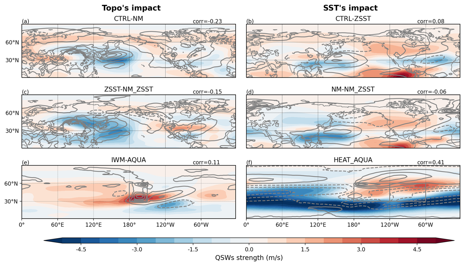
Figure 7 The same as Fig. 3, except for Eady growth rate at 700 hPa (contour; the interval is 0.1 per day).

3.2.3 Temporal analysis on Hypothesis 2

In Hypothesis 2, we have emphasized the importance of background conditions affecting QSW distribution using a linear framework with spatial analysis. However, there are limitations to this method, in which we have primarily relied on spatial correlations between QSWs and different variables in the CTRL and ERA5 simulations, and in differences between experiment pairs. To further explore this result, and the robustness of the evidence in support of Hypothesis 2, we extend the analysis into the temporal dimension.

Pearson correlation coefficients between QSW strength and $-|\mathrm{Ks}-\mathrm{6}|$ are computed over winter using data subsampled every 10 d to reduce autocorrelation, following White and Mareshet Admasu (2025). Significance is assessed using a false discovery rate adjustment. The broadly positive correlations in all experiments (Fig. 8) confirms that QSWs in many locations tend to be stronger during times when the Ks value in that location is closer to 6, further confirmation of the importance of Ks in modulating QSW strength. With longer time series in the experiments, correlations tend to be stronger and significant over broader regions than in ERA5, which shows broadly positive correlations, but with limited significance. While no significant correlation appears exactly where QSW strength peaks in CTRL, the significant regions largely coincide with areas of strong QSW activity. In AQUA, significant correlations even appear globally, further supporting the effectiveness of the Ks hypothesis. It is not surprising, however, that the Ks hypothesis fails in HEAT, likely due to the strong northward shift of jets in that configuration.

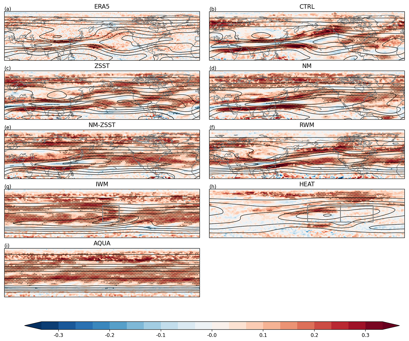
Figure 8 Temporal correlations between QSW strength and $-|\mathrm{Ks}-\mathrm{6}|$ in ERA5 (a), CTRL (b), ZSST (c), NM (d), NM-ZSST (e), RWM (f), IWM (g), HEAT (h), and AQUA (i). Shading indicates correlation values, with dotted regions denoting significance at p<0.05, adjusted for the false discovery rate. Data have been subsampled to once every 10 d to reduce autocorrelation. Contour lines represent QSW strength, with a 2 m s⁻¹ interval.

Whilst Fig. 8 broadly supports the hypothesis that Ks values closer to 6 lead to a higher probability of strong QSWs, this is not universally true. This leads us to ask whether nonlinear interactions among transient eddies themselves could explain the QSWs in some situations. To explore this, we examine the temporal correlations between transient eddy strength and QSW strength in Fig. A10. The significant negative correlations at QSW peaks in Fig. A10a, b, c, and f suggest a competitive relationship when topography is included; on the contrary, in experiments without topography – though less clear in IWM due to weak topographic forcing – QSWs and transient eddies tend to vary together temporally over almost all of the Northern Hemisphere. This helps explain why the contribution of transient eddies is generally smaller in topography-related experiment pairs: the nature of their covariation changes. Across ERA5 and all experiments, transient eddies and QSWs exhibit significant correlations over broad regions, supporting the possibility that transient eddies can become quasi-stationary in response to the supportive background conditions. Further investigation is needed to understand the spatial distribution of these temporal correlations.

4 Summary and discussion

In this study, we have examined the role of stationary forcings on the duration and climatological distribution of QSWS, including testing of two hypotheses, involving four variables that may shape the spatial distribution of QSWs. The stationary wavenumber, Ks, is the only variable for which there are high correlations with QSW strength in ERA5, CTRL, and all experiment pairs we studied (Table 2), suggesting that it can consistently help explain both the present day QSW distribution, and differences in the QSW spatial distribution between idealized experiments. The transient eddy strength has high correlations in most situations, but negative correlations for the experiment pairs IWM-AQUA and HEAT-AQUA. This suggests that the transient eddy strength can be important for QSWs, but is not the only factor. The Eady growth rate and stationary wave strength also show positive correlations with QSW strength in both CTRL and ERA5, but changes in these variables cannot explain the differences in many experiment pairs. Overall, our results support the hypothesis that background conditions based on stationary wavenumber, combined with the presence of transient eddies, can explain the spatial distribution of QSWs in many different climate configurations. This suggests that a simple barotropic interpretation of QSWs is sufficient for a broad understanding of their spatial and temporal distribution. This is not, however, evidence that baroclinic and/or non-linear dynamics do not also play a role in QSW dynamics.

It also worth noting that our results show that the correlations in ERA5/CTRL are not always indicative of the correlations in the changes for some factors. This underscores the caution needed when interpreting QSWs distribution in the real world. The complex interplay of forcings in reality makes isolating underlying mechanisms difficult, emphasizing the value of idealized experiments such as those performed in this study, and a model hierarchy in advancing our understanding of QSW dynamics.

In this study, for simplicity, we study QSWs at 200 hPa and chose not to employ a latitudinally varying wavenumber range, as in Wolf et al. (2018). To understand how these choices may have impacted our results and conclusions we compute QSWs for the CTRL, ZSST, and NM simulations at 300 hPa, and for different wavenumber ranges (see Fig. 9). The choice of pressure level between 200 and 300 hPa makes little difference for the CTRL simulation, or the differences between the CTRL and ZSST or NM (compare the top two rows in Fig. 9). Conversely, the choice of wavenumber does have some impact on the distribution of QSWs in the CTRL simulation (compare Fig. 8g and i), which can explain the difference between climatological QSWs in our results (e.g. Fig. 9a) compared to Fig. 2b in Wolf et al. (2018). However, the differences between the experiments, i.e., CTRL-ZSST and CTRL-NM, show little sensitivity to the choice of wavenumber (compare Fig. 9e with 9h and 9k, and similarly 9f with 9i and 9l), suggesting that these choices likely have relatively little impact on our main results and conclusions.

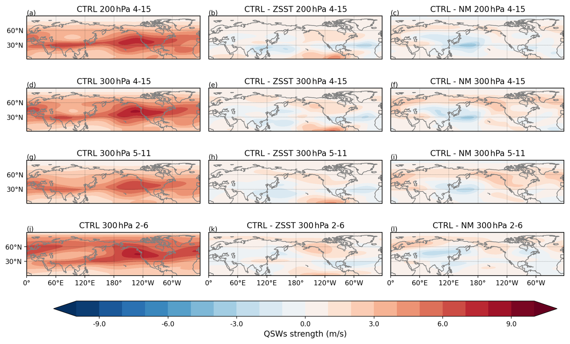
Figure 9 This figure illustrates the strength of climatological QSWs across various pressure levels and wavenumber ranges. The left column shows QSW strength in CTRL, the middle column shows the difference between CTRL and ZSST, and the right column shows difference between CTRL and NM. The first row shows QSW strength at 200 hPa with wavenumber 4–15, the second row is at 300 hPa with wavenumber 4–15, the third row is at 300 hPa with wavenumber 5–11, the second row is at 300 hPa with wavenumber 2–6.

Overall, our results show that the stationary wavenumber Ks and strength of transient eddies can explain a significant proportion of the spatial and temporal distribution of QSWs under many substantially different climates; however, this does not address the question of these QSWs' energy sources. Further analysis is needed to quantify and understand the energy sources and transfers involved in QSW dynamics. It would also be interesting to further explore the impact of zonal SST asymmetries in some cases, e.g. in a warming climate. This work focuses on the midlatitudes, which may overlook QSWs originating in the tropics – for example, those triggered by the MJO that can substantially influence QSW distribution (Fei and White, 2023).

The sensitivity to QSW timescale definition

To assess the robustness of our results to the definition of “quasi-stationary” that we use, we also calculated QSW strength using both a 15–30 d Lanczos band-pass filter and a 30 d Lanczos low-pass filter. The results (summarized in Table 3) indicate that the relationship between QSW changes and variations in the selected metrics remains relatively consistent across these distinct filtering approaches, particularly the strong correlations with Ks and transient eddies, for experiment pairs with realistic land. However, experiment pairs using the 15–30 d band-pass filter exhibit greater differences from the 15 d low-pass filter (given in Table 2) than from the 30 d low-pass filter, especially in correlations with Ks and transient eddy strength. This suggests potential differences in QSW behaviour across different timescales. The two experiment pairs with the lowest correlation coefficients with Ks for 15–30 d bandpass QSWs are NM-NM_ZSST, and IWM-AQUA. If we increase the timescale range to 15–45 d, these correlation coefficients increase from 0.17 to 0.26 and from 0.09 to 0.18 respectively, illustrating that the higher correlations in the 30 d band-pass filter are not solely from very low frequency signals. Nonetheless, the consistently high correlations with Ks and transient eddy strength in CTRL-ZSST and CTRL-NM, along with the positive correlations in ZSST-NM_ZSST and NM-NM_ZSST, suggest that quasi-stationary waves on both shorter (15–30 d) and longer (30–90 d) timescales share similar characteristics and governing mechanisms under semi-realistic conditions. In more idealized experiment pairs, different mechanisms may contribute to QSWs in varying proportions depending on their timescale. These findings broaden our understanding of QSW dynamics.

Table 3 The spatial correlations between QSW strength and different metrics in ERA5 and experiments within 15–75° N are presented. The left values represent the correlations using QSWs calculated with 15–30 d band-pass filtered meridional winds. The right values represent the correlations using QSWs with 30 d low-pass filtered meridional winds.

Overall, our results provide the most support for our second hypothesis – that transient eddies can become quasi-stationary under favorable background conditions, which can be identified through the stationary wavenumber, Ks. This does not, however, prove that the mechanisms proposed in Hypothesis 1 are completely invalid, or that non-linear processes do not also play a role in QSWs. Considering Hypothesis 1, related to the mechanism of QRA proposed by Petoukhov et al. (2013), this mechanism further requires the existence of a waveguide and the same phase for stationary waves and transient eddies. Our research tests only one aspect, the connection to stationary waves, and our conclusions are drawn solely from climatological statistics. For analyzing extreme events, the QRA framework may still provide a useful approach.

It could also be argued that Ks could impact both quasi-stationary and stationary waves similarly, as we find positive correlations between QSWs strength and Ks, and Ks is derived for stationary waves originally; however, the experiment pairs that show the strongest positive correlation between QSWs and Ks (CTRL – NM; CTRL-ZSST) notably do not show a strong correlation between QSWs and wavenumber 4–15 stationary wave strength in Table 2. Indeed the only experiment pair with a strong positive correlation between QSWs and wavenumber 4–15 stationary waves (HEAT-AQUA) has a nearly zero correlation between QSWs and Ks. Thus, stationary waves with wavenumbers 4–15 are not primarily affected by stationary wavenumber in the same way as QSWs; it is likely that changes in the forcing of stationary waves plays a direct role.

We have discussed how transient eddies contribute differently to QSW strength in experiment pairs reflecting the impact of topography versus zonal SST asymmetries, as shown in Sect. 3.2.2. This difference also varies with QSWs of varying durations. As shown in Table 3, correlations between Ks and QSW strength are generally higher for longer-duration QSWs (right column), except in experiments involving CTRL. In contrast, correlations between transient eddy strength and QSW strength tend to decrease with longer QSW durations, except in experiments involving NM_ZSST and IWM-AQUA. For experiment pairs involving diabatic heating changes – excluding HEAT – correlations remain high for QSWs lasting more than 30 d. This further suggests different mechanisms behind topographic and SST/diabatic heating impacts, though further analysis of QSW life cycle is necessary to confirm the processes of these mechanisms. Finally, the weaker Ks contribution to shorter-duration QSWs implies that nonlinear processes, such as interactions among transient eddies, may also generate QSWs.

5 Conclusions

In this research, we conducted eight CAM6 simulations with prescribed SSTs to understand the impact of stationary forcings: topography, zonal SST gradients, and land surface, on the characteristics of quasi-stationary waves. Comparison of our CTRL experiment with ERA5 reanalysis confirms that QSWs, and the associated variables that we study, are reasonably well replicated by the CAM6 model. Our findings reveal that:

1. the presence of topography, land, and/or SST gradients tends to extend the duration of QSW events

2. stationary forcings have a strong influence on the spatial distribution of climatological QSW amplitude

3. Changes in QSWs in response to stationary forcings are primarily associated with changes in the background flow conditions, as described by the stationary wavenumber, Ks, combined with changes in transient eddy strength

4. In all experiments, over much of the Northern Hemisphere, QSWs are stronger on days when the stationary wavenumber Ks is closer to 6, and when transient eddy strength is high

5. In experiments with topography, transient eddies and QSWs tend to exhibit a competitive relationship in some locations, particularly where the climatological QSW strength is high, whereas in experiments without topography, they tend to covary almost everywhere

6. The stationary wavenumber Ks and transient eddy strength are still important when QSWs are defined on different timescales, but may have different relative importance for different timescales of QSW

This work helps further our understanding of QSWs underlying mechanisms, which may help better understand biases in QSW forecasts, and provides insights into future changes in QSW strength and associated uncertainties under global warming – any changes in transient eddy strength and/or the stationary wavenumber Ks, will likely lead to changes in QSWs.

Appendix A: Additional figures

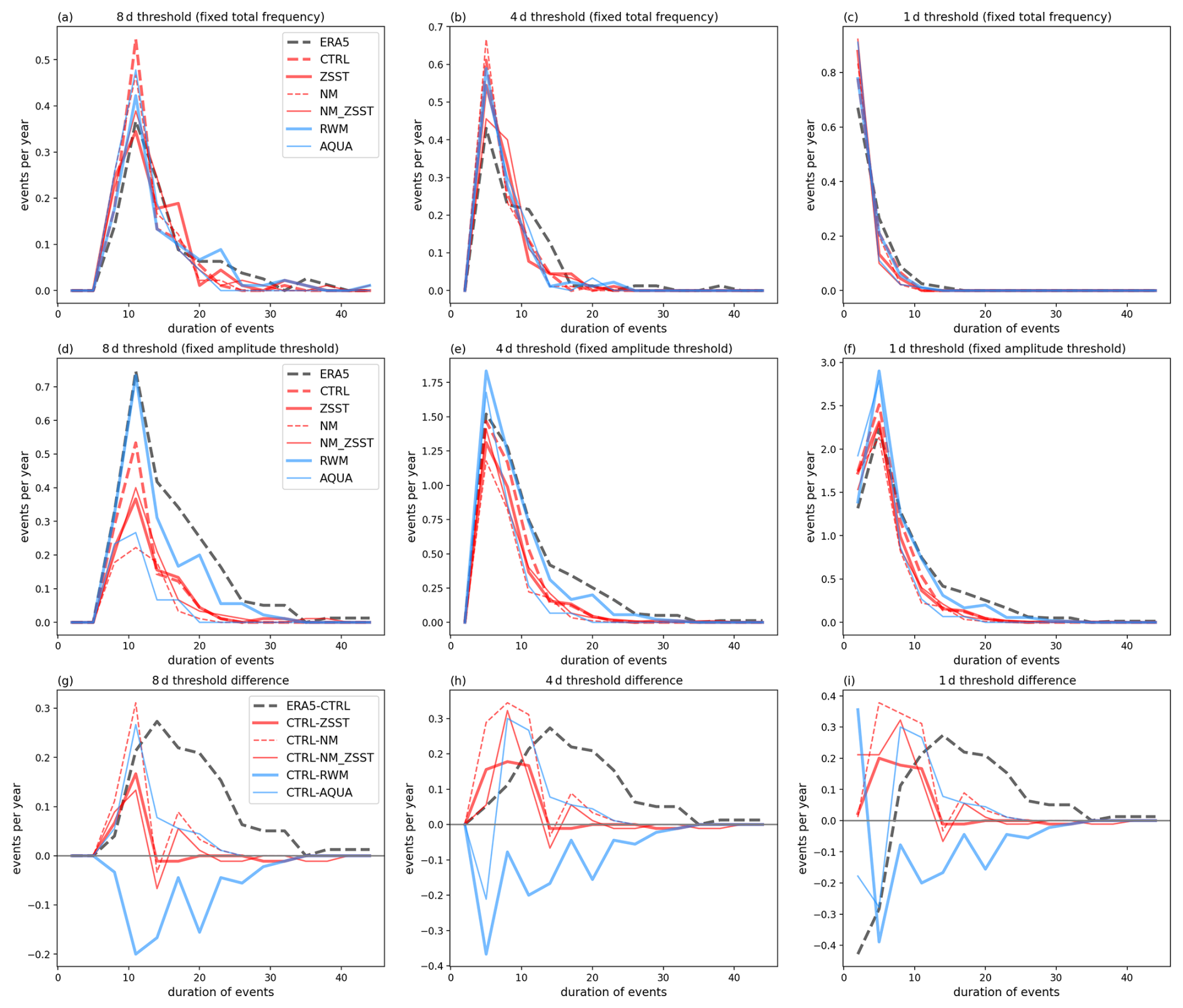
Figure A1 This figure shows statistics in Europe (0–60° E). The first row is same as the first row in Fig. 1, and the third row is the same as the bottom row in Fig. 1. In the second row, the threshold for QSW events is determined based on event frequency, allowing it to vary across simulations in order to maintain a fixed event frequency across all simulations and ERA5.

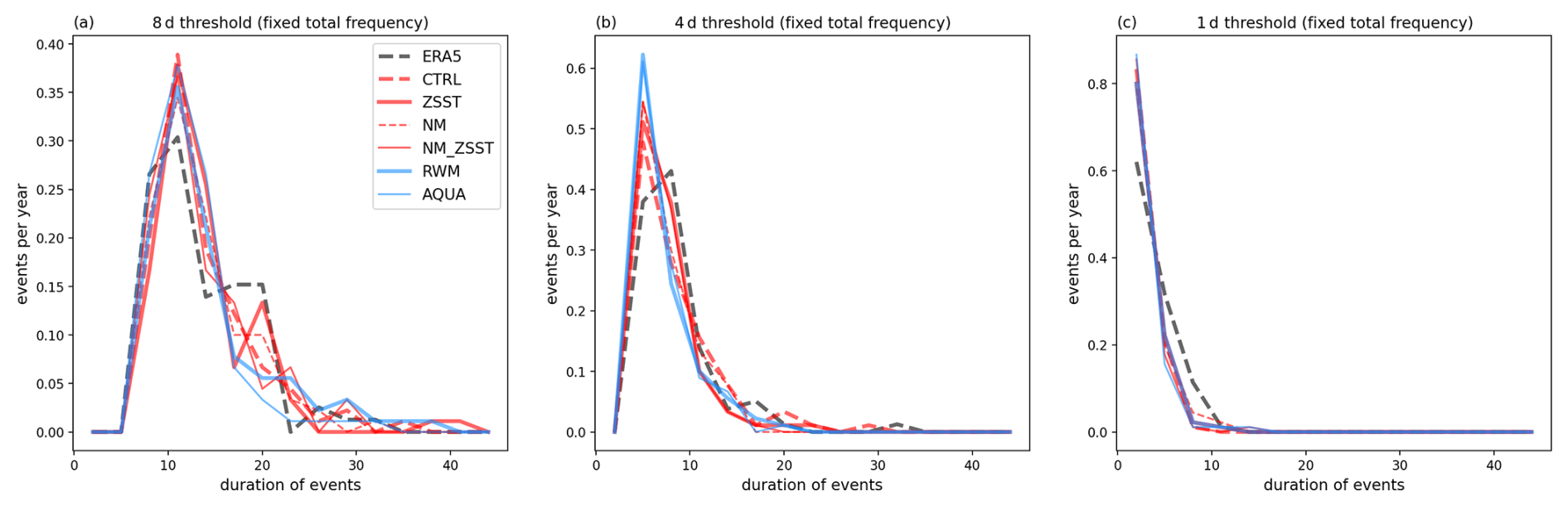
Figure A2 The same as the second row in Fig. A1, except for North American (120–60° W) events.

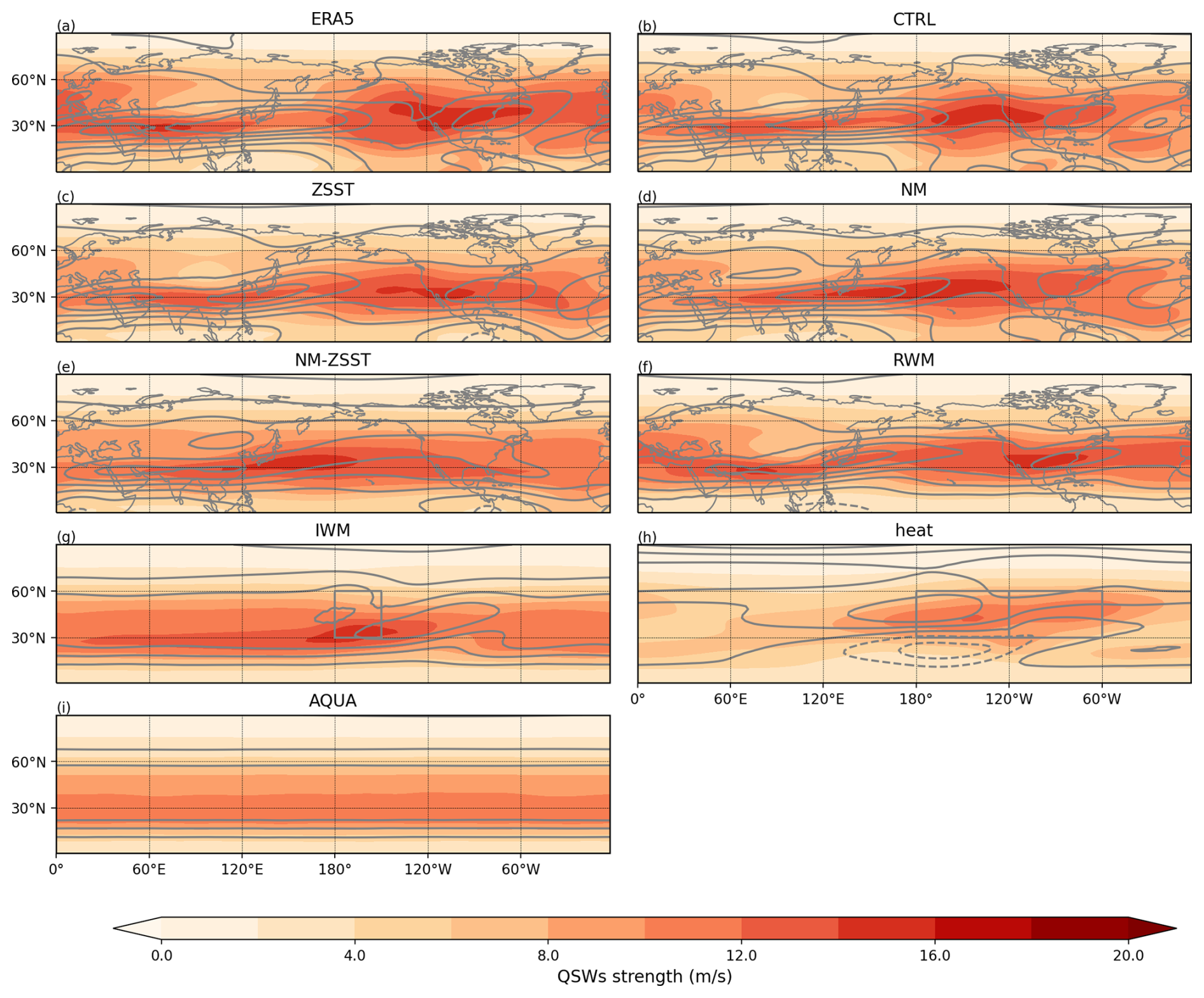
Figure A3 Climatological QSW amplitude in winter (shading) and climatological zonal wind (contour) in ERA5 (a) and idealized experiments – CTRL (b), ZSST (c), NM (d), NM-ZSST (e), RWM (f), IWM (g), HEAT (h), and AQUA (i). The line spacing is 4 m s⁻¹, solid lines represent westerlies and zero contour whilst dashed lines represent easterlies. The ERA5 reanalysis time range is from 1940 to 2014, and the time range of idealized experiment is 100 years.

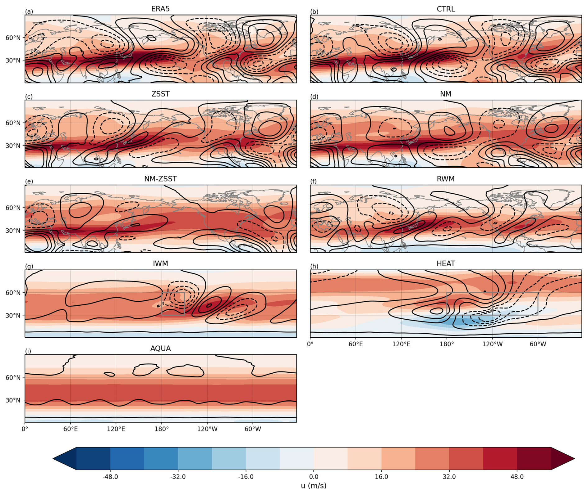
Figure A4 Climatological zonal wind in winter (shading) and climatological meridional wind (contour). Other information is the same as Fig. A3.

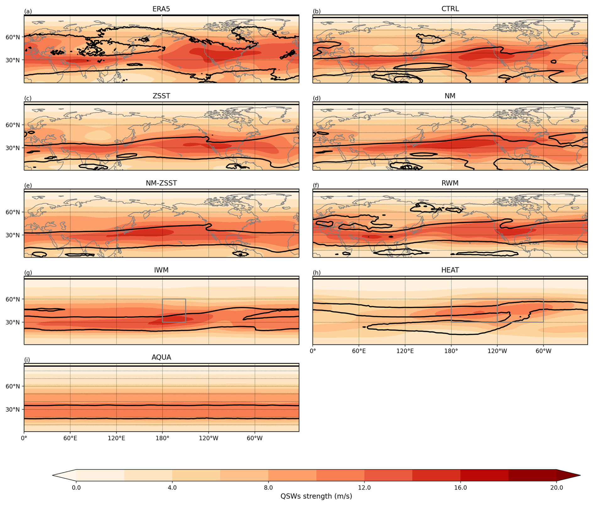
Figure A5 Climatological QSW strength in winter (shading) and stationary wavenumber Ks=4 and Ks=8 (contour). Other information is the same as Fig. A3.

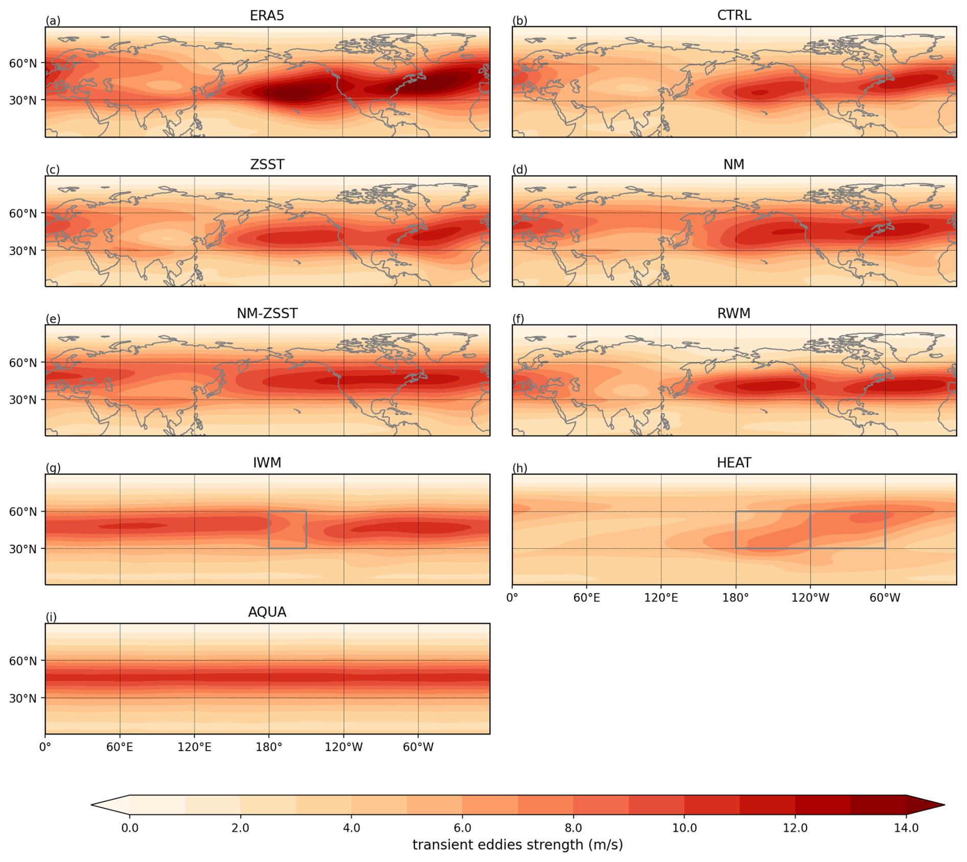
Figure A6 This figure shows climatological transient eddy strength. Other information is the same as Fig. A3.

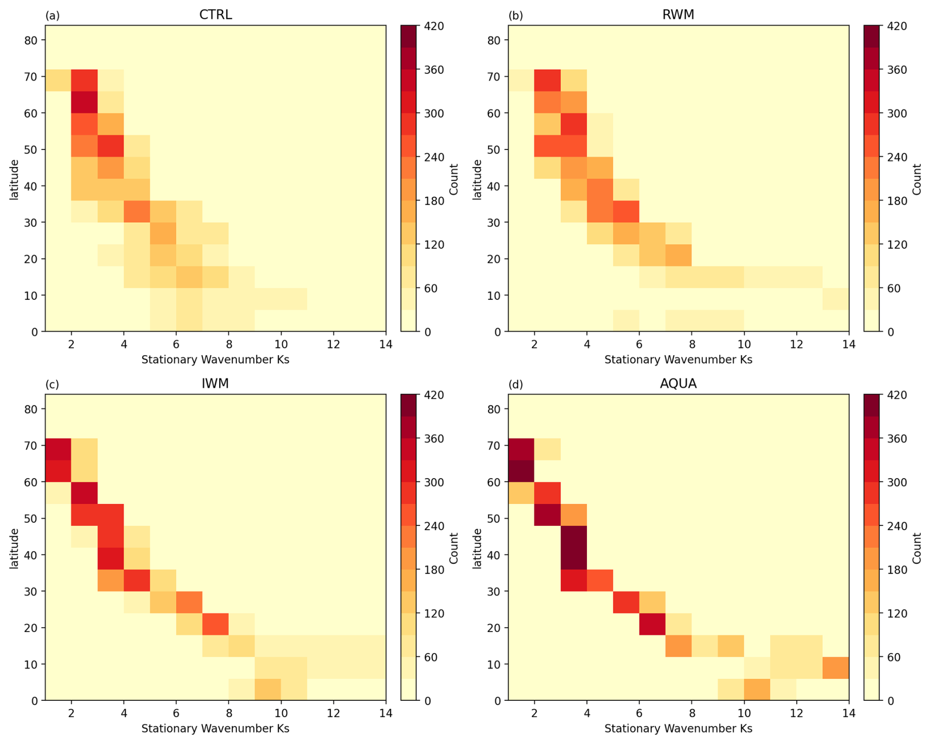
Figure A7 Heatmap showing the number of grid points in winter (DJF) climatology that climatological stationary wavenumber Ks is x at latitude y. (a) shows the statistics in CTRL, (b) for RWM, (c) for IWM and (d) for AQUA.

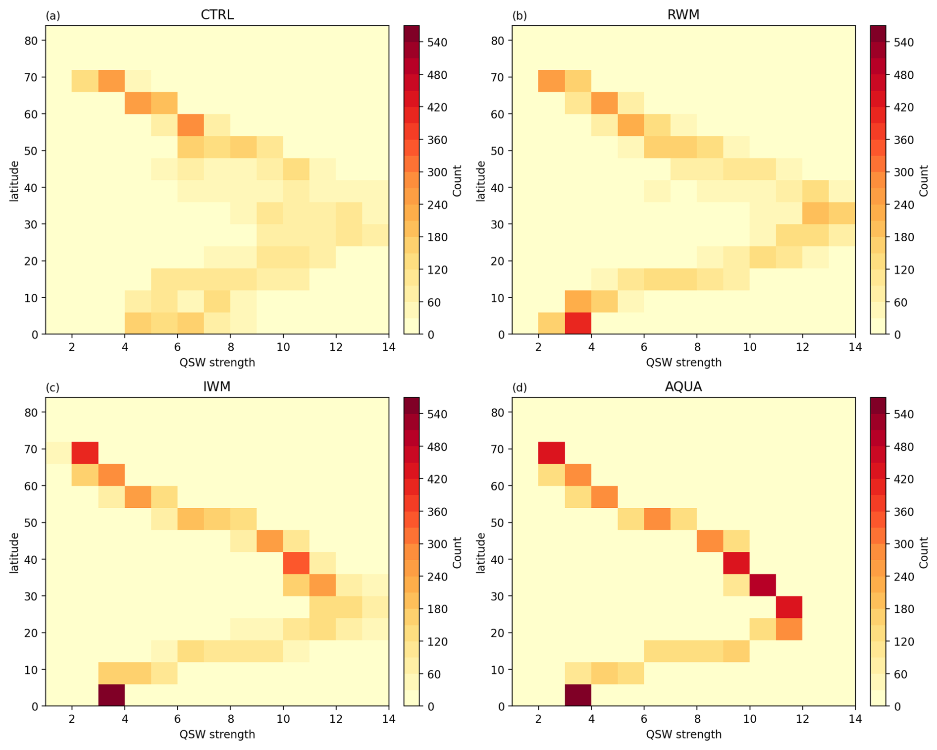
Figure A8 Heatmap showing the number of grid points in winter (DJF) climatology that QSW strength is x at latitude y. (a) shows the statistics in CTRL, (b) for RWM, (c) for IWM and (d) for AQUA.

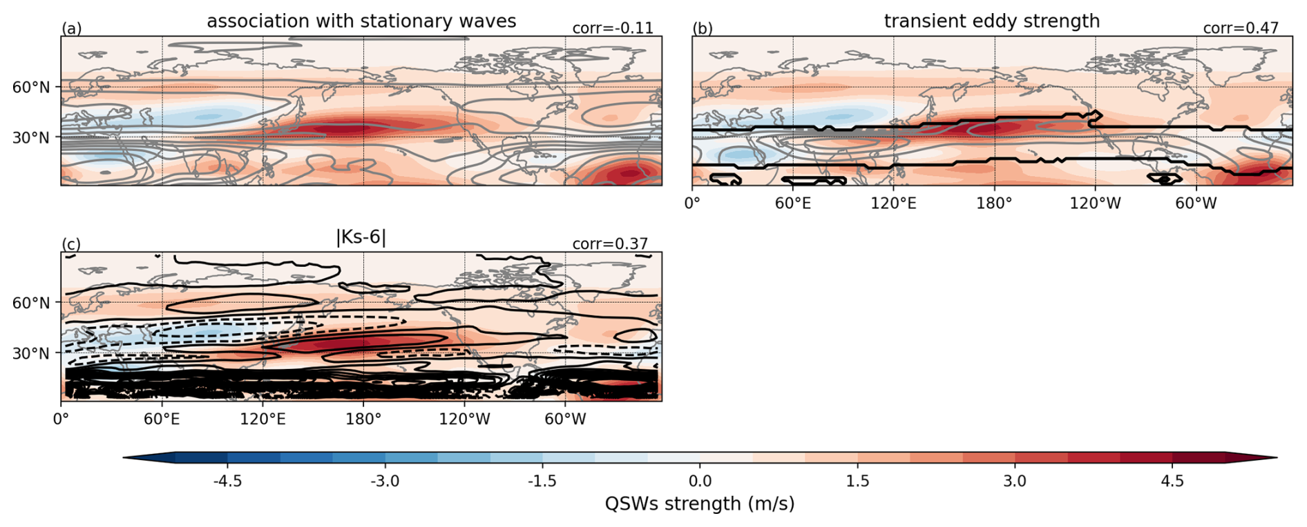
Figure A9 The difference between NM-ZSST and AQUA showing the impact of land surface. Climatological QSW strength (shading) and climatological wavenumber 4–15 stationary wave strength (contour) in (a), climatological transient eddy strength (contour) in (b), How much the stationary wavenumber Ks deviated from Ks=6 (contour) multiplied by −1 in (c).

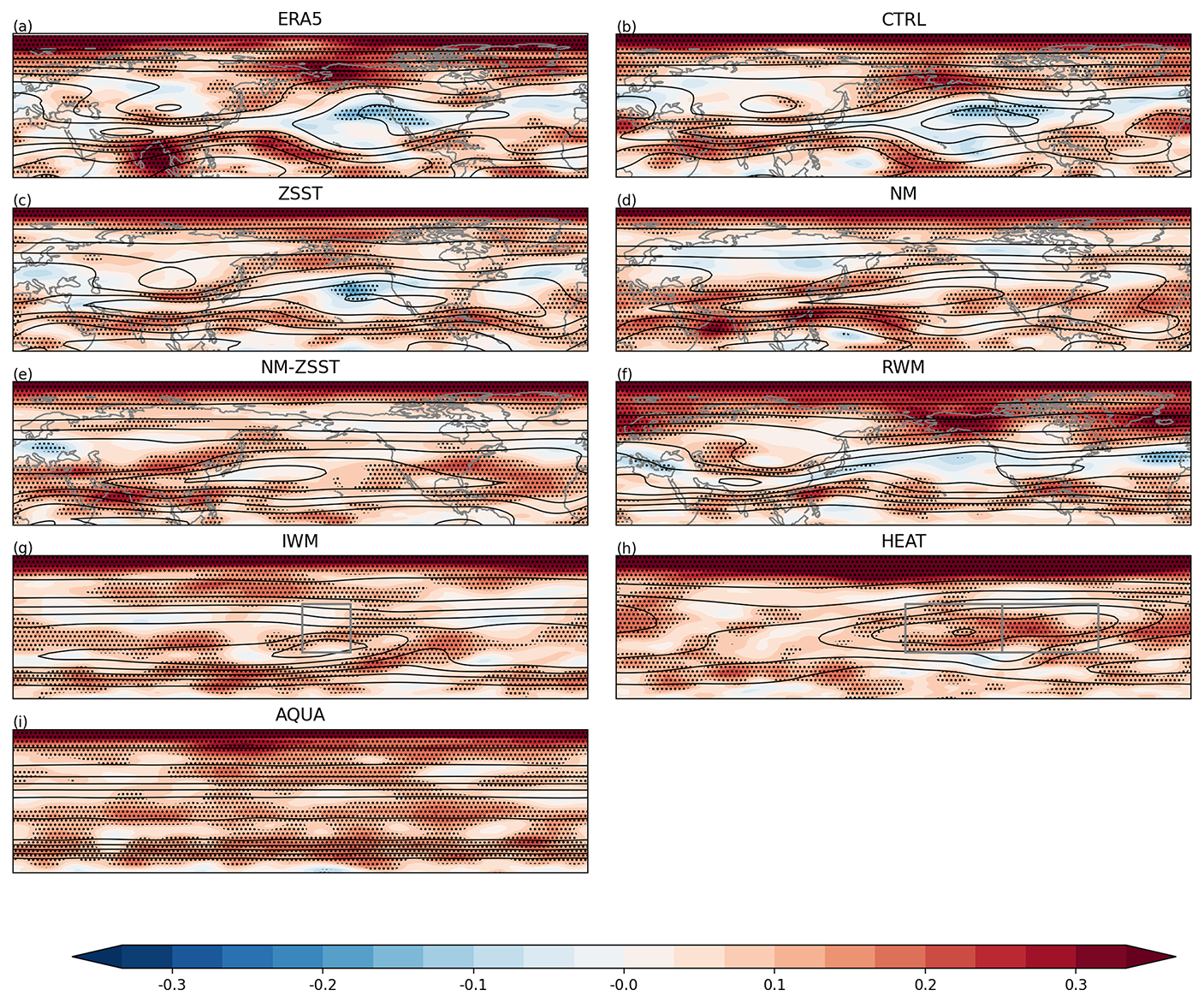
Figure A10 This figure shows the temporal correlations between QSW strength and transient eddy strength. Other information is the same as Fig. 8.