A climatology of atmospheric rivers over Scandinavia and associated precipitation

Atmospheric rivers (ARs) play an important role in the global climate system, facilitating both meridional moisture transport and regional weather patterns that are important for the local water supply. While previous research has mainly focused on the relationship between ARs and precipitation in North America and East Asia, the role of ARs in the regional climate of Scandinavia remains understudied. In this study, we used data from the Atmospheric River Tracking Method Intercomparison Project to characterize ARs making landfall in Scandinavia during 1980–2019. Combined with ERA5 reanalysis precipitation data, we quantified the AR-related precipitation over the region. We found that ARs are present during up to 5.9 % of the time in the most active areas over Denmark and southern Norway. During these AR events, some locations receive up to 40.7 % of their total annual precipitation. Additionally, ARs are more strongly associated with higher precipitation rates compared to non-AR events. By clustering the ARs using a k-means algorithm, we identified four typical AR pathways over Scandinavia (maximum annual AR frequencies and AR-related precipitation fraction in parentheses): over southern Denmark (4.2 %, 19.7 %), along the northern coast of Norway (2.6 %, 13.1 %), over the southern parts of Norway and the south-central parts of Sweden (2.0 %, 15.1 %), and along the southern coast of Norway (1.1 %, 7.8 %). Furthermore, we found that ARs over Scandinavia are typically most common during autumn and least frequent in spring, with some differences in seasonality between AR pathways. To investigate how large-scale atmospheric circulation affects Scandinavian ARs, we used the North Atlantic Oscillation (NAO) index to characterize circulation patterns during AR events. We found that AR activity over Scandinavia generally peaks during strong positive phases of the NAO (> 1.5). Our results indicate that ARs over Scandinavia, despite being relatively infrequent, are associated with a large fraction of the annual precipitation, emphasizing their important role in the regions's weather and climate.

1 Introduction

Atmospheric rivers (ARs) are long, but narrow, temporary pathways of unusually high atmospheric moisture transport that significantly influence precipitation patterns in many mid-latitude regions (e.g., Ralph and Dettinger, 2011). Globally, ARs are estimated to account for a majority of the poleward moisture transport (Zhu and Newell, 1998), and play an important role in the local climate of many regions (e.g., Guan and Waliser, 2019). However, despite their widespread importance, ARs and their impacts on Scandinavian weather and climate have received limited scientific attention.

In ARs, moisture is transported long distances from mid-latitude ocean basins toward higher latitudes, passing over ocean and land (Zhu and Newell, 1998; Ralph et al., 2004). This long-range transport is a result of interactions between dynamical processes within the warm conveyor belt of extratropical cyclones (Gimeno et al., 2014). Here, in the pre-cold-frontal zone, the strong temperature gradient across the front results in a strong low-level jet, which combined with local moisture convergence and poleward moisture transport produces the intense moisture transport found within ARs (e.g., Ralph et al., 2005; Bao et al., 2006).

ARs are an established feature in mid-latitude weather and climate. Along the west coast of North America, ARs are present for up to 13 % of the time annually (Rutz et al., 2014; Guan and Waliser, 2019). These ARs are associated with up to 50 % of the coastal precipitation (e.g., Ralph et al., 2004, 2005; Rutz and Steenburgh, 2012; Dettinger et al., 2011; Guan and Waliser, 2015), and have been linked to ending many persistent droughts in the region (Dettinger, 2013). In South, Southeast, and East Asia there are up to 32 AR days per year (∼ 9 % of the time) on average, where ARs contribute to around 30 % of the annual precipitation depending on the region (Liang and Yong, 2021). ARs over Asia have also been linked to more than 50 % of the most extreme precipitation days during the year (Liang and Yong, 2021; Kim et al., 2021). In Western Europe, the maximum annual AR frequencies reach 13 % over the British Isles and parts of Norway, Spain, and Portugal (Guan and Waliser, 2019). Along these more coastal areas, AR-related precipitation contributes up to 30 % of the annual total precipitation (Lavers and Villarini, 2015), and has been linked to many of the most impactful precipitation events (e.g. Lavers and Villarini, 2013; Lavers et al., 2012; Ionita et al., 2020). With the projected increases in temperature during the 21st century, AR frequencies are expected to increase at many of the previously mentioned locations (e.g., Ramos et al., 2016; Zhang et al., 2024; Shields et al., 2023; Hagos et al., 2016; Lavers et al., 2013), and as a result increase the importance of ARs in the climate of high-latitude regions. Hence, increasing our understanding of the patterns and future changes of ARs is vital for improving predictions of regional hydrological extremes.

Studies like the ones described above, investigating ARs on a regional to global level, commonly rely on some type of computerized detection of ARs in gridded datasets, such as reanalysis products or the output from climate models. Here, ARs are typically identified using a variable that describes the total amount of water vapour that is transported in the atmospheric column, such as the vertically integrated water vapour transport (IVT), in combination with an AR detection and tracking algorithm (ARDT). These algorithms typically operate by applying a threshold on the IVT field, either a fixed value a variable value derived from, e.g., a climatological quantile, to generate the initial selection of spatially continuous features of high IVT values. ARs are then identified by applying additional filtering criteria to these thresholded IVT regions, including constraints on geometric properties such as the length and width, average IVT direction, and temporal persistence. However, this relatively open choice when it comes to IVT threshold and the properties used in the filtering has resulted in a large variety of ARDTs from the scientific community. To quantify the differences among the ARDTs, the Atmospheric River Tracking Method Intercomparison project (ARTMIP; Shields et al., 2018) provides a common set of experiments on which the ARDTs can be evaluated and subsequently compared. One of the initial findings of the ARTMIP project is that there is a large spread in the AR detection rate among the participating ARDTs (Rutz et al., 2019). It is therefore recommended that studies should make use of multiple ARDTs whenever possible (Shields et al., 2023).

Previous studies focusing on ARs over Scandinavia found that up to 8 of the 10 strongest precipitation events along the coast of Norway were related to ARs (Lavers and Villarini, 2013), and that moisture sources at low latitudes played an important role during extreme precipitation events (Stohl et al., 2008). However, a detailed climatology of AR activity over Scandinavia outlining the seasonality and local trends of ARs, as well as their spatial variations, is currently not available. Similarly, a descriptive view of the AR–precipitation relationship in the region is lacking.

Hence, this study is focused on Scandinavia with the objectives to:

• 1.

  Quantify the contribution of ARs to regional precipitation.

• 2.

  Identify the different pathways of ARs that make landfall.

• 3.

  Characterize the seasonal variability of AR activity.

• 4.

  Examine the relationship between large-scale circulation and AR occurrence.

To accomplish this, we analysed all ARs between 1980 and 2019 identified by four different ARDTs from the ARTMIP AR catalogue: GuanWaliser_v2, Mundhenk_v3, TempestLR, and Reid500.

Section 2 describes the methodology and data used in this study. In Sect. 3 and the following subsections, we present and discuss the results. Section 3.1 presents the annual AR frequencies over Scandinavia, along with estimates of AR-related precipitation. In Sect. 3.2, we examine the frequencies of the four identified AR pathways over Scandinavia and their influence on regional precipitation. Section 3.3 and 3.4 then analyse the seasonality of these pathways and their relationship with large-scale circulation patterns, respectively. Section 3.5 discusses uncertainties and differences between ARDTs. Finally, Sect. 4 summarizes the main findings and conclusions of the study.

2 Methods

2.1 Data

In this study, we analysed AR characteristics over Scandinavia using four AR catalogues published by the ARTMIP project (Shields et al., 2018; Collow et al., 2022): GuanWaliser_v2, Mundhenk_v3, TempestLR, and Reid500 (details in Table 1). We included all available AR catalogues based on the ERA5 reanalysis product (0.25° × 0.25°, Hersbach et al., 2020) that provide global spatial coverage and span 1980–2019 at hourly resolution. Note that at the time of writing, although ERA5 reanalysis data are available through 2025, the AR catalogues published by ARTMIP extend only to the end of 2019. For our analysis we downsampled the AR catalogues to a 6-hourly resolution to improve the computational efficiency, which is in line with previous studies (e.g.,  Zhou et al., 2018; Guan and Waliser, 2017; Arabzadeh et al., 2020; Mattingly et al., 2018). We also used the 6-hourly accumulated total precipitation from the same ERA5 reanalysis product to analyse the influence of ARs on precipitation.

Guan and Waliser (2015, 2019)Mundhenk et al. (2016)McClenny et al. (2020)Rhoades et al. (2020)Ullrich and Zarzycki (2017)Reid et al. (2020)

Table 1 ARDTs used in the study and their IVT thresholds.

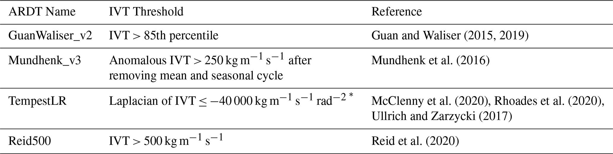
^* Does not capture points with IVT ≤ 250 kg m⁻¹ s⁻¹ (McClenny et al., 2020).

ARDTs can be divided into two groups based on if they use a fixed or variable IVT threshold. ARDTs with fixed thresholds apply a constant value across the entire spatial domain, e.g., IVT ≥ 500 kg m⁻¹ s⁻¹. For the ARDTs used in this study, only the Reid500 ARDT is classified as using a fixed threshold. Variable threshold ARDTs employ a threshold that vary spatially and, in many cases, by season. For the remaining three ARDTs participating in this study, this is achieved in three different ways: GuanWaliser_v2 uses percentiles, Mundhenk_v3 uses anomalies above a fixed threshold, and TempestLR uses a fixed threshold applied to the Laplacian of the IVT field.

2.2 Identifying Scandinavian ARs

The four AR catalogues share a common grid and temporal resolution, and were subsequently processed in the same way. In the following sections, this workflow will be described for a single AR catalogue, but it was applied to all four catalogues. We then aggregated the results of the four AR catalogues, creating a catalogue ensemble, from which we derived the results of this study.

In the AR catalogues provided by the ARTMIP project, each time step contains a binary mask composed of contiguous regions, or “blobs”, that delineate ARs identified by the respective ARDT. We will refer to each unique AR “blob” in a time step as an AR object. To filter out the individual AR objects that make landfall in Scandinavia, we performed the following steps: First, we separated the AR objects within each binary mask by applying a connected component algorithm that identifies and labels distinct contiguous areas (4-connectivity). Each individual AR object was assigned a unique identifier. Second, we filtered for AR objects that intersect Scandinavia, defined as the geometric union of Denmark (excluding Greenland), Norway, and Sweden. To smooth out the irregular coastline and account for ARs that may influence regional precipitation without directly intersecting land at the grid point level, the land shape was buffered in two steps using the GEOS buffer algorithm: first by 0.85° latitude/longitude, and second by −0.15°. Figure 1 shows an overview of Scandinavia and the buffered region. Any AR object that spatially intersected this buffered version of Scandinavia was marked as making landfall. We limited the study domain to 50–74° N and 10° W–45° E, as AR segments extending beyond this region were considered to have negligible impact on the characteristics of Scandinavian ARs. This also came with the added benefit of lowering the computational requirements. Third, we tracked the AR objects that make landfall in Scandinavia backward in time, which is described next.

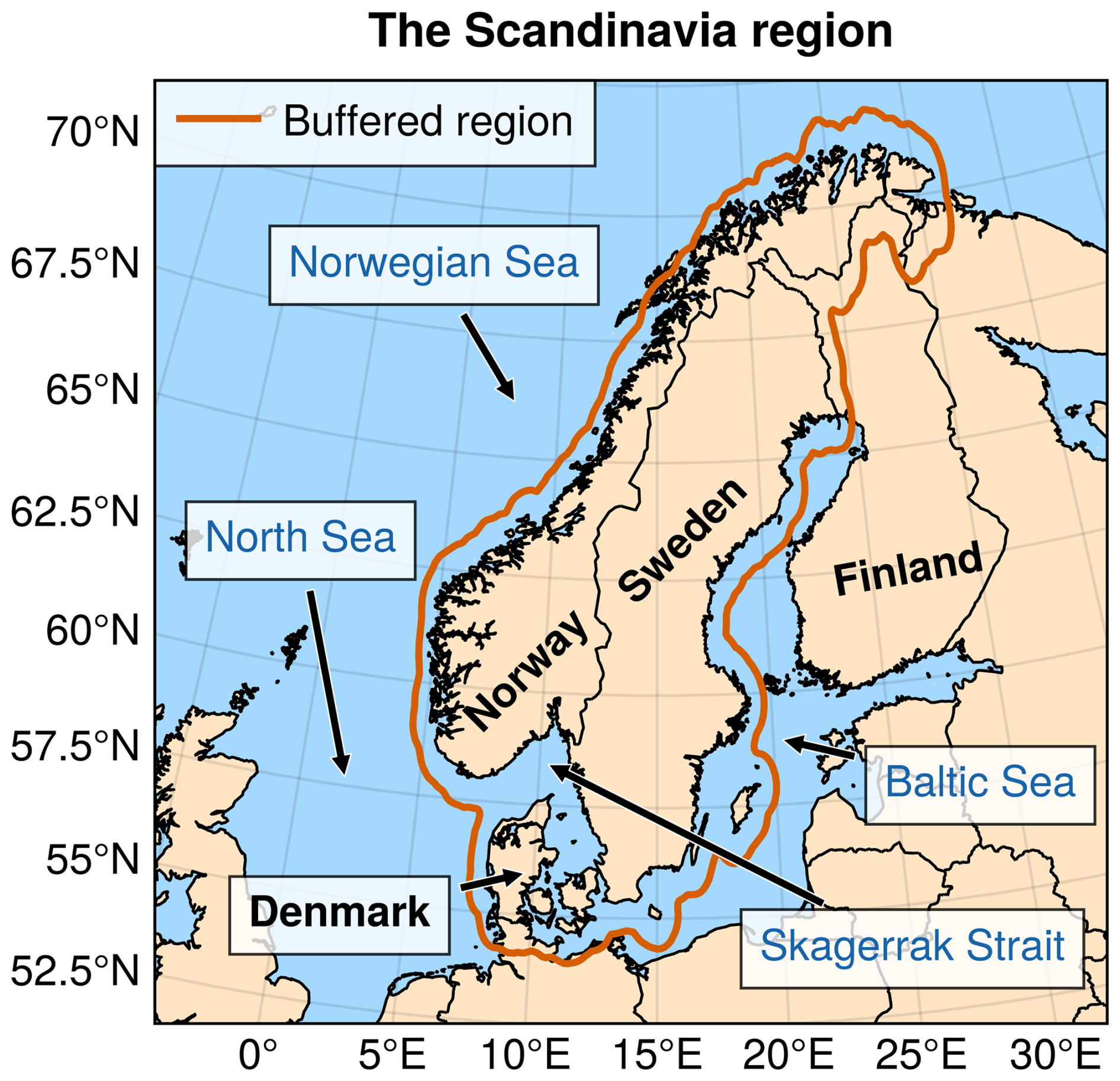
Figure 1 Map of the study region, here defined as the geometric union of Denmark, Norway, and Sweden. The red-orange line outlines the buffered region which was used to identify ARs that intersect Scandinavia. The approximate geographical positions of locations referenced later in the paper are also featured in the map.

The ARTMIP AR catalogues do not contain information about the temporal relationships between AR objects across consecutive time steps. Thus, to track ARs over time, we developed a method to identify which AR objects in different time steps belong to the same AR event. Our tracking algorithm uses an iterative approach, similar to the one described in Guan and Waliser (2019). At each time step, the algorithm compares every AR object to all AR objects from the previous time step and finds the most similar pairings. This pair is then considered as part of the same AR event. Following Guan and Waliser (2019), we computed the morphological similarity of the AR objects using an area-weighted Jaccard index (as described in Deza and Deza, 2016). This metric measures the fraction between the intersection and union of two binary AR objects:

$$\begin{array}{}\text{(1)}& J={\displaystyle \frac{|\text{A}\cap \text{B}|}{|\text{A}\cup \text{B}|}},\end{array}$$

where A and B are two AR objects from separate time steps. The vertical bars denote the absolute value operator. The Jaccard index is 0 for two objects with no intersection, and 1 for objects that completely overlap. An AR object in the current time step is considered a possible continuation of any previous AR object that returns a positive Jaccard index. In the case when more than one AR object has a non-zero Jaccard index with a single AR object from the previous time step, the AR object with the highest Jaccard index is considered its continuation. Similarly, if an AR object has a non-zero Jaccard index with multiple AR objects from the previous time step, the AR object with the highest index is considered its origin. If an AR object has no overlap with any AR objects in previous time steps, it is considered a new AR and will be kept for future iterations of the tracking algorithm. Our approach differs from that of Guan and Waliser (2019) in that we performed the tracking on the binary AR masks from ARTMIP rather than on the IVT field. Furthermore, we also allowed the size of the look-back during tracking to iteratively increase from 6 up to 24 hours if no matching ARs were found. This was done to account for the possibility of AR objects missing in a time step due to for example geometry constraints of the ARDT. Hence, if two overlapping AR objects are separated by e.g. 12 h with no AR object in-between, they were still considered to be part of the same AR event.

Finally, we summed all temporally linked AR objects to create composite ARs representing the full lifecycle of individual AR events. These composite ARs were then used to analyse the general AR characteristics over Scandinavia, such as frequencies and trends, as well as in the identification of common AR pathways.

2.3 Clustering ARs

To investigate the possible recurring patterns of AR pathways over Scandinavia, we categorized the composite ARs using k-means clustering, analysing each AR catalogue separately. The k-means algorithm requires the user to specify the numbers of clusters that should be fit to the data. To find the optimum number of clusters we evaluated the sample silhouette scores from two to ten clusters (see Figs. A11–A14). We found the optimal number of initial clusters to be different depending on the AR catalogue: four for GuanWaliser_v2 and Mundhenk_v3, and six for Reid500 and TempestLR.

The clusters were initialized and fit using the “Scalable K-Means++” algorithm described in Bahmani et al. (2012) and implemented in the Python library Dask-ML. After the initial fit, we observed that some of the clusters in Reid500 and TempestLR exhibited high spatial correlation. To consolidate these clusters, we computed the spatial correlation between each cluster and the four clusters of Mundhenk_v3, which served as a reference. This resulted in four clusters for each AR catalogue, which were re-ordered based on their spatial correlation with the Mundhenk_v3 clusters. These clusters represent the common pathways of ARs that make landfall in Scandinavia. From here on, the clusters will be referred to as AR pathways, or simply pathways.

2.4 ARs and regional precipitation

To investigate the relationship between ARs and precipitation in Scandinavia, we identified all time steps during which ARs make landfall in Scandinavia. Based on the AR time steps we calculated the AR-related precipitation by subtracting the average non-AR precipitation from the precipitation during AR events, while also constraining AR precipitation to be non-negative. The non-AR precipitation was calculated using time steps when no ARs were present over Scandinavia. We then computed both total annual AR-related precipitation and average 6-hourly precipitation rates for all AR events and for each AR pathway. To evaluate the spatial co-location between ARs and precipitation, we computed the field correlations between AR frequency and precipitation patterns.

2.5 Grouping AR pathways by season and NAO index

To examine the variability of ARs and AR-related precipitation, we grouped the ARs by the assigned pathway and the season. Here, we used the standard meteorological season definitions: December–January–February (DJF), March–April–May (MAM), June–July–August (JJA), and September–October–November (SON). Each AR was assigned a season based on the time when it first made landfall in Scandinavia.

Finally, we investigated the relationship between AR frequency and the North Atlantic Oscillation (NAO), which is the leading mode of atmospheric circulation variability over the North Atlantic and Northern Europe (e.g., Hurrell and Deser, 2010). We used the normalized daily NAO index from the Climate Prediction Centre (NOAA Climate Prediction Center, 2025) to represent the phase of the NAO. The daily mean NAO index was assigned to each AR based on the first time the AR made landfall in Scandinavia. The ARs were then categorized based on their AR pathway and five NAO index bins: strong negative (NAO < −1.5), negative (−1.5 ≤ NAO < −0.5), neutral (−0.5 ≤ NAO ≤ 0.5), positive (0.5 < NAO ≤ 1.5), and strong positive (NAO > 1.5). For each NAO bin and AR pathway combination, we computed the average AR frequencies by counting the total number of AR time steps and dividing it by the total number of time steps in the corresponding NAO bin. To further quantify changes in the distribution of AR frequencies across different NAO phases, we calculated the mean Wasserstein distance between the five frequency distributions. For each AR pathway, we calculated the pairwise Wasserstein distances between each NAO bin and all other bins, then averaged these values to obtain a scalar measure representing the overall change in the frequency distribution.

3 Results and discussion

The analysis outlined in the methods resulted in four separate sets of results, one for each AR catalogue, of annual AR frequencies, AR pathways, and AR-related precipitation estimates. We refer to these four results as the catalogue ensemble and present the ensemble median values, along with the range spanned by the lowest and highest member within brackets.

3.1 Annual AR frequencies and AR-related precipitation over Scandinavia

In the median of the catalogue ensemble, ARs that make landfall in Scandinavia are, in the most active subregions, present for up to 6 % [1 %–11 %] of the time during an average year (Fig. 2a). At the same time, these ARs are at some locations associated with up to 41 % [10 %–58 %] of the annual average precipitation, corresponding to 1139 mm [282–1568 mm] (Fig. 2b, c). Specifically, the subregions with the highest AR-related precipitation fraction are found along the southwest coast of Norway and the west coast of Denmark. Furthermore, we note that over Scandinavia in its entirety, the minimum AR-related precipitation fraction is 12 % [3 %–18 %]. The AR frequency and precipitation patterns are moderately well aligned, with a median field correlation of 0.46 across all AR catalogues.

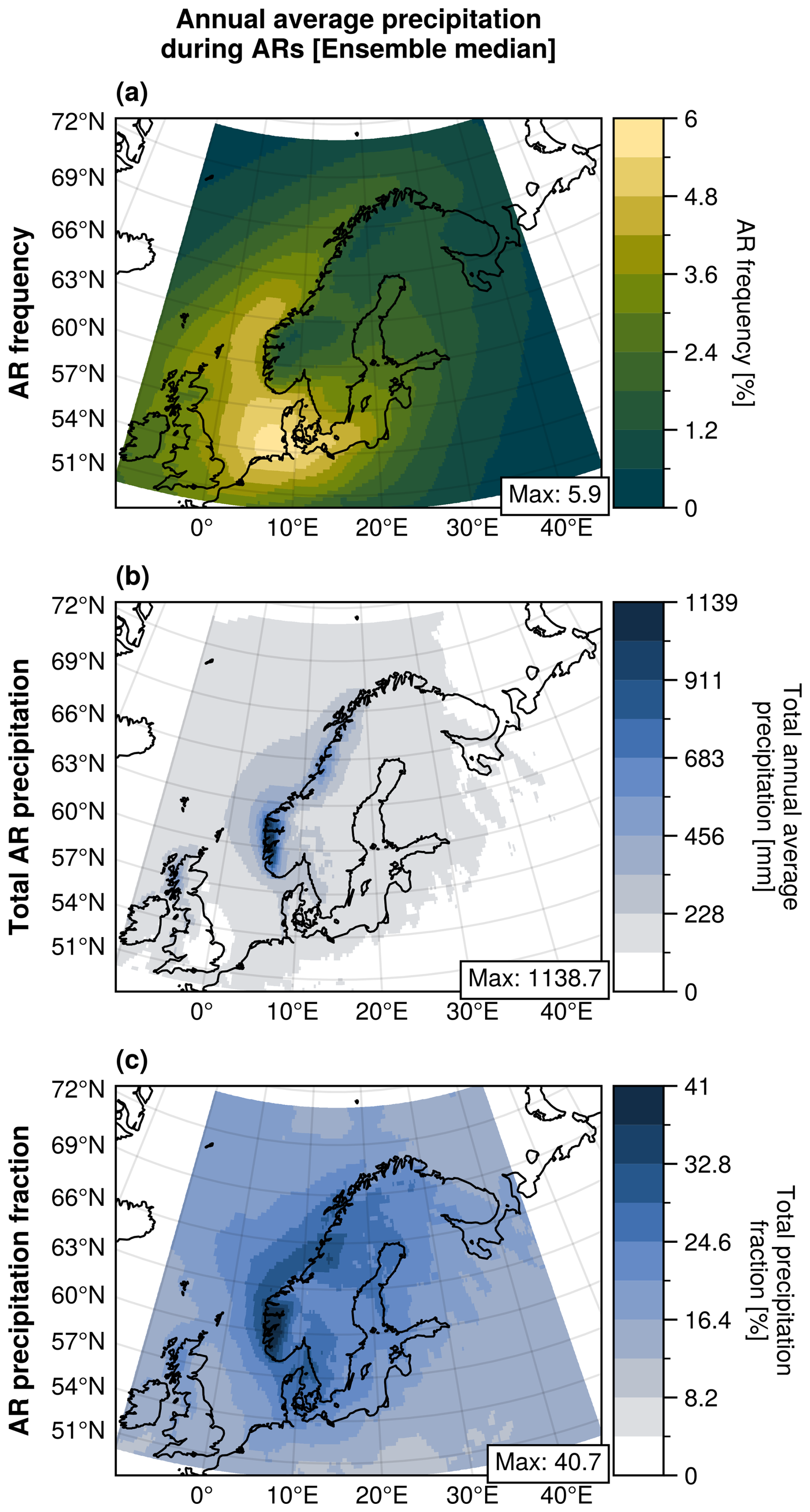
Figure 2 (a) Annual average AR frequency, (b) annual total AR-related precipitation, and (c) fraction of total precipitation attributed to ARs over Scandinavia between 1980 and 2019. All values represent the median of the catalogue ensemble, which comprises four AR detection algorithms: Mundhenk_v3, GuanWaliser_v2, Reid500, and TempestLR. Both the AR frequency and precipitation aggregates are based on ERA5 reanalysis data.

Compared to the AR frequency maximum, the location of the maximum AR-related precipitation is shifted further north, toward the Norwegian southwest coast. This difference can likely be explained by orographic effects: Norway's mountainous terrain enhances AR precipitation through orographic lifting (e.g., Roe, 2005), while Denmark's relatively flat topography allows ARs to reach further inland (e.g., Rutz et al., 2014).

To further examine the relationship between the annual AR frequency and precipitation, we computed the annual frequencies of ARs making landfall anywhere over Scandinavia and compared these with the spatial average of annual precipitation and AR-related precipitation over the same region (Fig. 3). The catalogue ensemble median shows that ARs intersect Scandinavia between 16 % and 29 % (2.5th–97.5th percentiles) of the time during the year. For the ensemble maximum, these numbers increase to between 36 % and 54 %, while staying below 10 % for the ensemble minimum. Single ARs intersecting Scandinavia were most common, with multiple ARs intersecting the region simultaneously during only 2 % of the year. These relatively high AR frequencies compared with the lower spatial AR frequencies in Fig. 2 indicate that ARs intersect Scandinavia via different pathways.

The total annual AR frequency is moderately correlated with the annual total precipitation (light blue bars in Fig. 3) over Scandinavia, with an ensemble median r value of 0.46 [0.35–0.48], all significant at p < 0.05. Unsurprisingly, the total AR frequency is strongly correlated to the annual total AR-related precipitation, with an r value of 0.92 [0.88–0.98]. Furthermore, the correlation between the regional annual total precipitation and AR-related precipitation is high, with a significant (p < 0.05) r value of 0.68 [0.40–0.77].

We investigated the trends in the annual AR occurrence using the Mann–Kendall trend test, and did not find any trends significant at the 0.05 level for any of the AR catalogues.

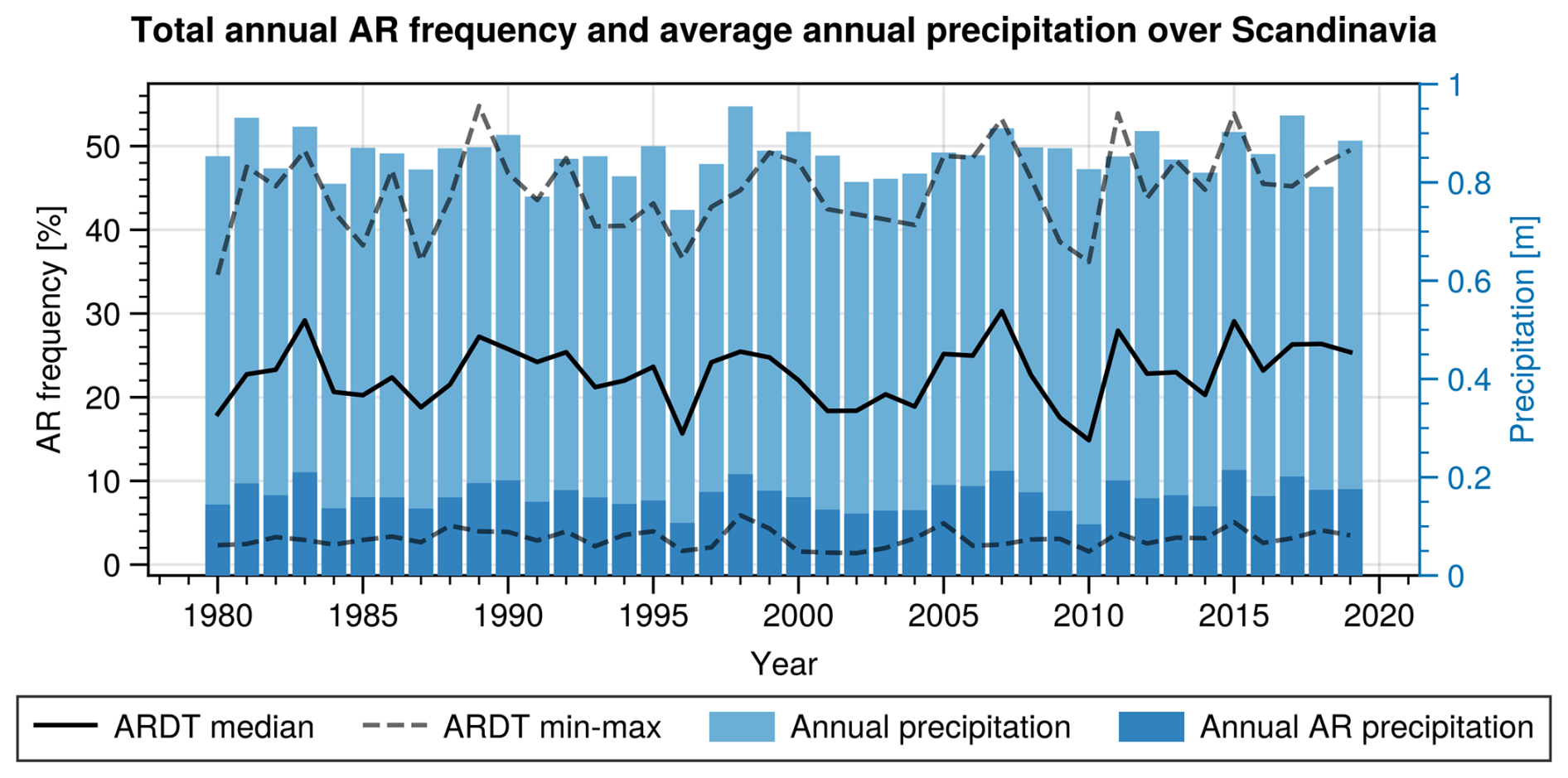
Figure 3 Time series of total annual AR occurrence and annual precipitation over Scandinavia. The black solid line shows the catalogue ensemble median AR occurrence, while the dashed lines show the catalogue ensemble minimum and maximum. The light blue and dark blue bars, both starting from zero, represent the spatial averages of annual total precipitation and AR-related annual total precipitation, respectively.

Comparing the 6-hourly accumulated precipitation during AR and non-AR events, we find that spatially averaged precipitation rates are generally lower during ARs in the catalogue ensemble median (Fig. 4a). If we instead look at the catalogue ensemble maximum, precipitation rates ≥ 0.66 mm 6 h⁻¹ are more common during ARs. We also examined the spatial maximum of precipitation to understand how ARs influence the more intense precipitation over the region (Fig. 4b). Here, our results indicate that precipitation rates ≥ 12 mm 6 h⁻¹ are more common during AR events, even in the catalogue ensemble minimum.

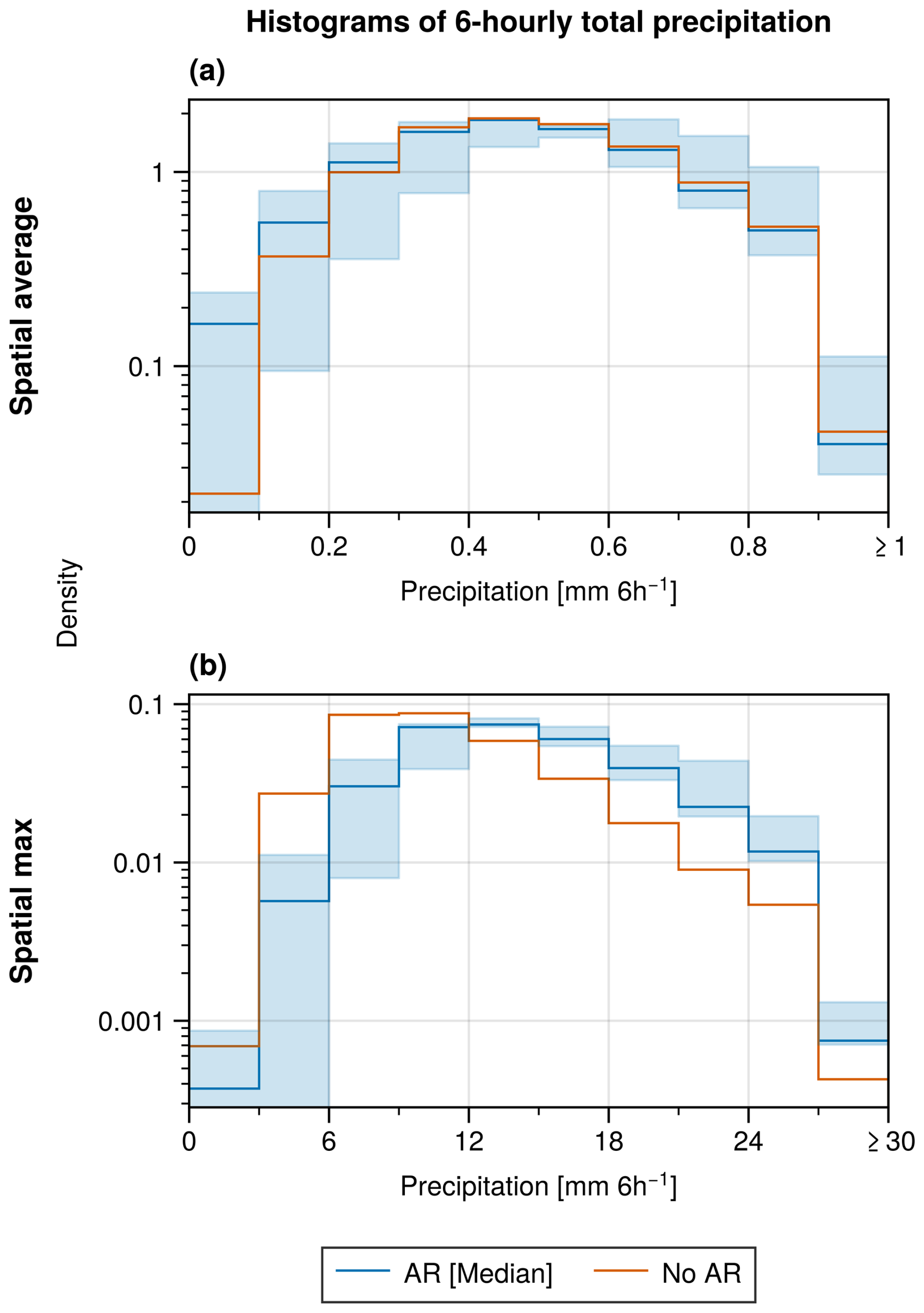
Figure 4 Distributions of the spatial (a) average and (b) maximum 6-hourly accumulated precipitation during AR (blue) and non-AR (red-orange) events. The rightmost bins in the histograms are open-ended, encompassing all values (a) ≥ 0.9 mm 6 h⁻¹ and (b) ≥ 27 mm 6 h⁻¹. Shading indicates the full range of the ensemble for the AR conditions.

3.2 Primary AR pathways over Scandinavia

We identified four AR pathways that represent the primary routes by which ARs make landfall in Scandinavia. Similarly to the preceding analysis, the clustering was done on each AR catalogue separately, and the results were combined into an ensemble. The ensemble median annual average AR frequency and AR-related precipitation for each AR pathway are shown in Fig. 5.

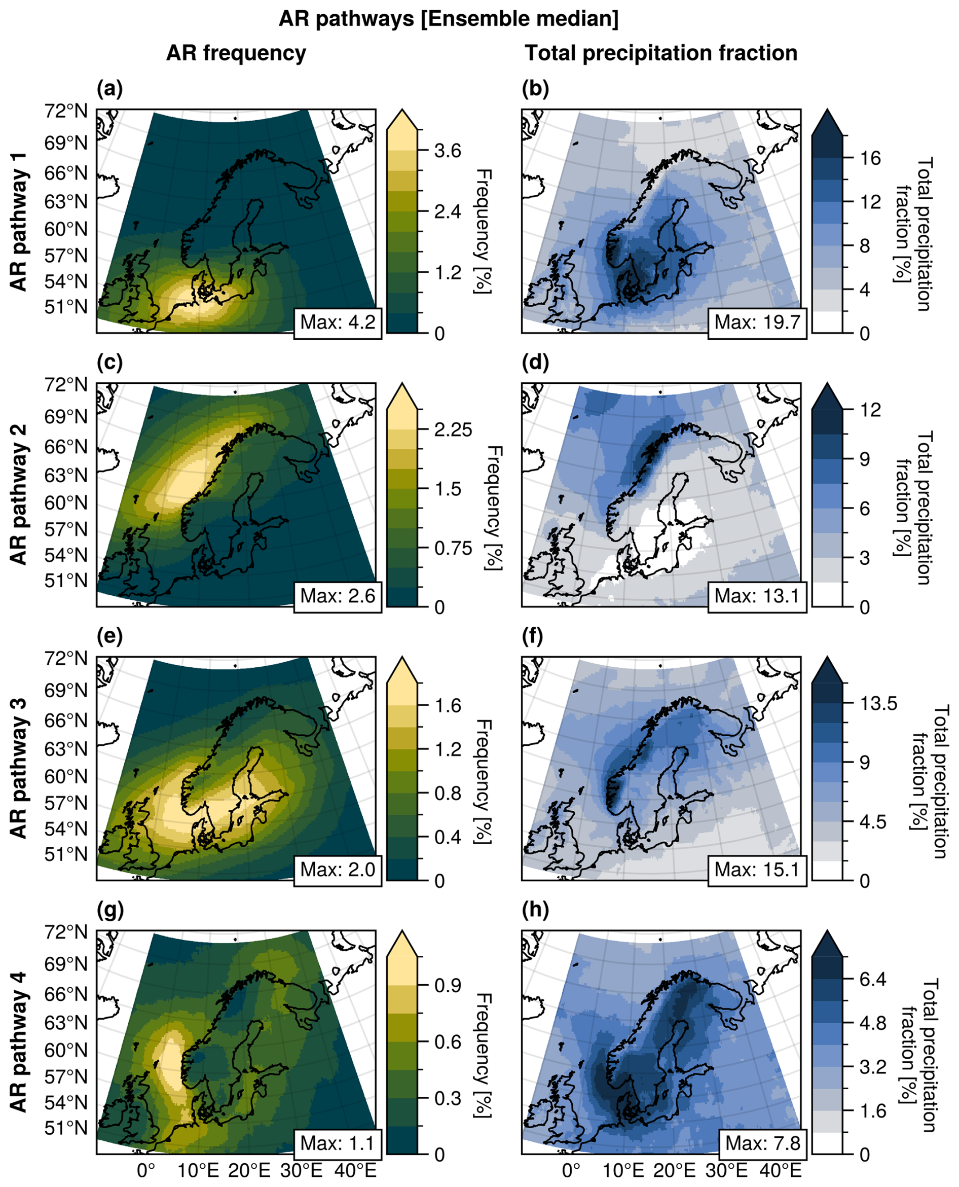
Figure 5 Ensemble median annual average AR frequencies (a, c, e, g) and total precipitation fraction (b, d, f, h) for each identified AR pathway (rows). Note that the colour scales differ between the subplots.

The southernmost ARs are found in pathway 1 (Figs. 5a, A3a, A4a). This is the most common pathway for ARs reaching Scandinavia, with annual frequencies reaching up to 4.2 % [0.9 %–5.0 %], or ∼ 15 d. Here, the AR frequency maximum is located mostly outside Scandinavia, in the region between Denmark and Northern Germany. Pathway 1 is also where we find the highest AR-related precipitation (19.7 % [6.7 %–25.0 %]; Figs. 5b, A3b, A4b). Compared to the AR frequency pattern, the pattern of AR-related precipitation is shifted slightly to the north, over Denmark and southern Sweden, but the field correlation between the patterns remains moderately high: 0.52 [0.34–0.67].

AR pathway 2 (Figs. 5c, A3c, A4c) consist of ARs that make landfall along the northern west coast of Norway. These ARs occur up to 2.6 % [0.4 %–4.4 %] of the time during an average year (∼ 9 d), with the maximum frequencies over the Norwegian Sea, and are related to a maximum of 13.1 % [3.1 %–16.0 %] (Figs. 5d, A3d, A4d) of the annual precipitation in the area. This pathway shows the highest field correlation between the AR frequency and precipitation patterns: 0.62 [0.50–0.75].

In pathway 3, ARs are located along the southern west coasts of Norway, Sweden, and Denmark, with ARs also extending further inland over Sweden (Fig. 5e). During the average year, these ARs occur up to 2.0 % [0.4 %–6.0 %] of the time (∼ 6 d; Figs. 5e, A3e, A4e). Here, the AR-related precipitation accounts for up to 15.1 % [3.6 %–27.1 %] (Figs. 5f, A3f, A4f) of the total annual precipitation. The area of high AR-related precipitation corresponding to pathway 3 is shifted slightly to the north compared to the AR frequency pattern, resulting in a relatively low field correlation of 0.37 [0.06–0.76] between AR frequency and precipitation patterns. The ARs in pathway 3 are also a good example of the topographical constraints imposed by the Norwegian mountain range on AR propagation; the ARs appear to be blocked from propagating over the Norwegian mountains, and instead traverse the North Sea and the Skagerrak Strait toward the Swedish west coast, where the flat topography enables the ARs to penetrate further inland and even reach the Baltic Sea and beyond.

AR pathway 4 (Figs. 5g, A3g, A4g) includes ARs that mainly occur west of Denmark's west coast and Norway's southwest coast, with a predominant south-to-north orientation. This pathway exhibits some overlap with pathway 3, but the ARs in pathway 3 have a more west-east orientation. The ARs in pathway 4 are relatively infrequent, and are only present for up to 1.1 % [0.2 %–1.5 %] of the time (or ∼ 3 full days in a year). Despite this, the ARs in pathway 4 are related to a relatively large fraction of the total annual precipitation in the area of high AR frequency: up to 7.8 % [1.4 %–10.0 %] (Figs. 5h, A3h, A4h). Furthermore, for pathway 4 we find that the field correlation between the AR frequency and precipitation patterns is relatively high: 0.48 [0.44–0.56].

3.3 Seasonality of AR pathways over Scandinavia

The AR frequencies, and to some extent location, of the identified AR pathways vary throughout the year. In the following section we present the seasonal AR frequencies for each AR pathway. The frequencies represent the fraction between the number of AR time steps during each season and the total number of time steps in the respective season.

For all AR pathways except pathway 4, ARs are the least frequent during the spring (MAM, Fig. 6b, f, j, n), while autumn (SON) is overall the most active AR season (Fig. 6d, h, l). In pathway 1, AR activity is high throughout most of the year, with peak AR frequencies reaching at least 2.6 % [0.5 %–4.2 %] (Figs. 6a–d, A5a–d, A6a–d) during all seasons. These southernmost ARs still exhibit a weak seasonal cycle, characterized by a dip in the AR activity during spring (MAM), followed by a gradual increase in AR activity towards autumn (SON), where AR frequencies reach up to 5.4 % [1.8 %–5.7 %]. We also find this pattern in the monthly total AR frequency for pathway 1, where most AR catalogues shows a valley during April and May (Fig. 7a). In the ensemble maximum, the high AR frequency areas during summer and autumn are located further towards the east over the Baltic Sea (Figs. 6c, d, A6c, d).

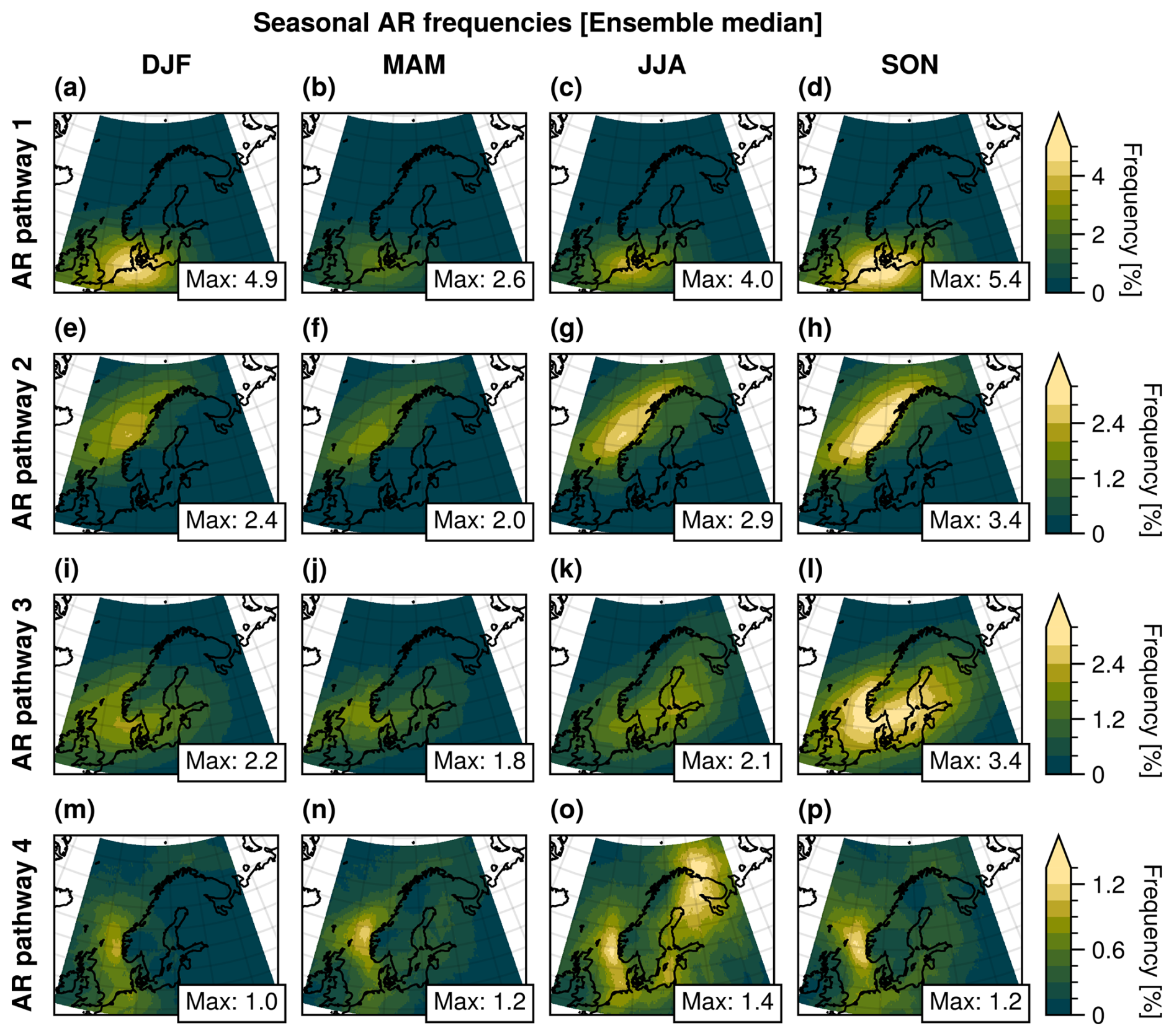
Figure 6 Maps of the average AR frequencies (ensemble median) during the seasons: winter (DJF), spring (MAM), summer (JJA), and autumn (SON) for each AR pathway. The frequencies correspond to the fraction of AR time steps relative to the total number of time steps within each season. Note that the colour scales differ between AR pathways (rows).

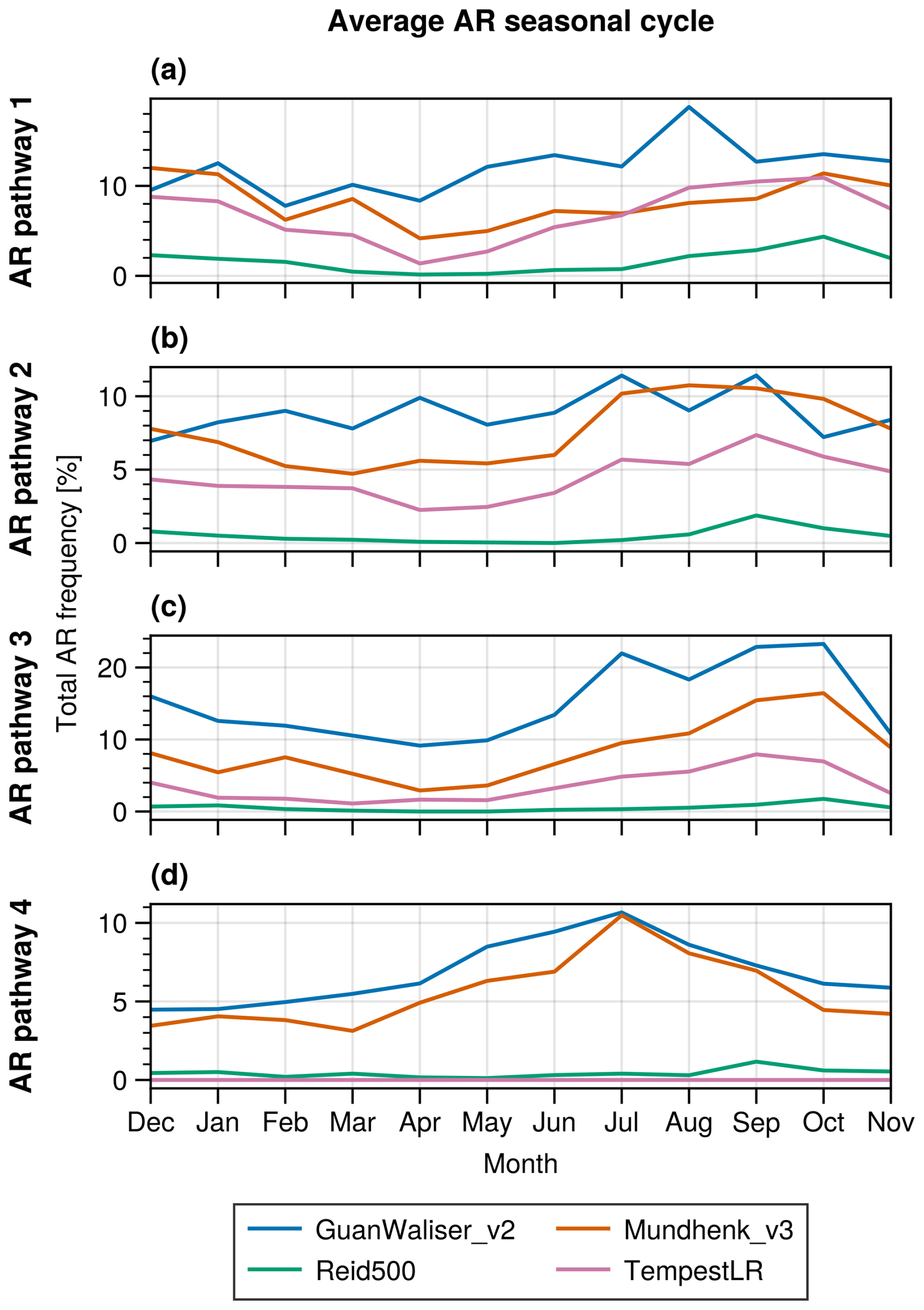
Figure 7 Average monthly total AR probability for the four AR pathways (rows). Each line represents a single AR catalogue: GuanWaliser_v2 (blue), Mundhenk_v3 (red-orange), Reid500 (green), and TempestLR (pink).

Pathway 2 shows a minimum in AR activity during spring (MAM), where AR frequencies reach 2.0 % [0.6 %–4.3 %] over a small area over the Norwegian Sea (Fig. 6f). During winter (DJF), the AR frequencies in this region are slightly higher and reach 2.4 % [0.8 %–4.5 %]. However, the area of high frequencies is small compared to the areas of high frequencies during both summer (JJA) and autumn (SON). For these two seasons, AR frequencies reach 2.9 % [0.8 %–4.8 %] over a long stretch of the Norwegian coastline (Figs. 6g, h, A5g, h, A6g, h). This seasonality is also visible in the monthly total AR frequency for pathway 2, with two AR catalogues (Mundhenk_v3 and TempestLR) showing an increase in AR activity during the summer months, followed by a slow decrease towards the minimum in April and May (Fig. 7b). This seasonal cycle is not as noticeable in GuanWaliser_v2, which exhibits a period of slightly increasing activity during summer, followed by a series of valleys and peaks during the rest of the year.

Similar to pathway 2, AR activity in pathway 3 peaks during the autumn. Here the area of high AR frequencies extends from the British Isles, across Sweden, and towards Finland, with AR frequencies reaching 3.4 % [1.2 %–8.4 %] (Figs. 6i–l, A5i–l, A6i–l). Following autumn, ARs are less frequent during winter and reach their minium during spring. Comparing the AR activity during winter and summer, the area of high AR frequency is shifted from the North Sea and Skagerrak Strait further east over the mainland of Sweden and the Baltic Sea (Fig. 6i, k). For pathway 3, the monthly total AR frequencies show a distinct peak during September and October in all AR catalogues except Reid500 (Fig. 7c).

The ensemble median AR activity in pathway 4 is relatively low throughout the year but shows a slight increase during summer (JJA), when frequencies reach ∼ 1.4 % [0.3 %–2.0 %] (Figs. 6m–p, A5m–p, A6m–p). Similarly, the monthly total AR frequency shows a clear seasonal cycle for two AR catalogues (GuanWaliser_v2 and Mundhenk_v3), with low activity throughout most of the year but with a clear peak in July (Fig. 7d).

3.4 Influence of NAO on AR pathways

Finally, we examined the relationship between the NAO and the frequency of AR pathways. Figure 8a–e shows the atmospheric circulation patterns during the different NAO phases, displaying daily average geopotential height for the neutral phase and geopotential height anomalies for the non-neutral phases. The AR frequencies for each NAO bin and AR pathway combination in Fig. 8f–y represent the relative AR occurrence during the respective NAO phase. Overall, the four pathways show the highest AR activity during strong positive phases of the NAO (> 1.5; Fig. 8j, o, t, y). In contrast, the magnitude of AR activity during the weaker phases of the NAO varies among the pathways. For pathway 1, we see relatively high AR frequencies for all phases of the NAO, with the highest frequencies during the strong positive phase. These ARs are the least frequent during the negative phase of the NAO, where frequencies reach 3.4 % [0.9 %–5.2 %] (Figs. 8g, A7g, A8g). Interestingly, ARs in pathway 1 appear more frequently during the strong negative phase of the NAO compared to the negative, neutral and positive phases, especially in the catalogue ensemble maximum (Fig. A8f–i). The NAO-grouped AR distributions for pathway 1 show moderate changes between all groups except the strong positive phase, as seen by the mean Wasserstein distance (Fig. 9).

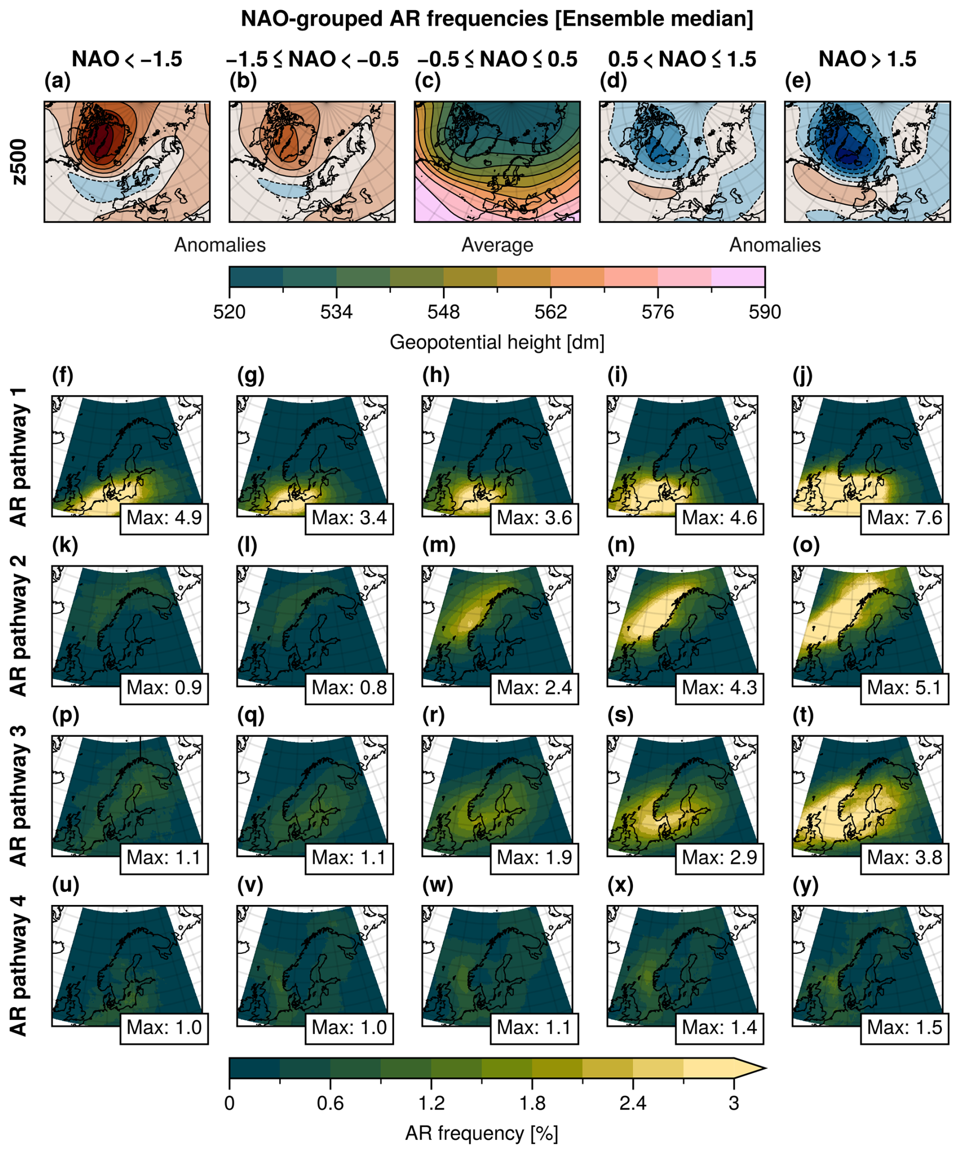
Figure 8 (a–e) Maps of 500 hPa geopotential height over the North Atlantic region during the different phases of the North Atlantic Oscillation (NAO). Panel (c) displays the mean geopotential height during the neutral phase. Panels (a), (b), (d), and (e) show geopotential height anomalies relative to the neutral phase, with contours every 5 dm starting at ±2 dm. Positive anomalies are shown with solid lines and red shading, while negative anomalies are shown with dashed lines and blue shading. (f–y) Corresponding AR frequencies (ensemble median) over Scandinavia for each AR pathway and NAO phase. Note that the colour scale of the AR frequency is capped at 3 %, with the maximum frequency value for each subplot is displayed in the bottom-right corner.

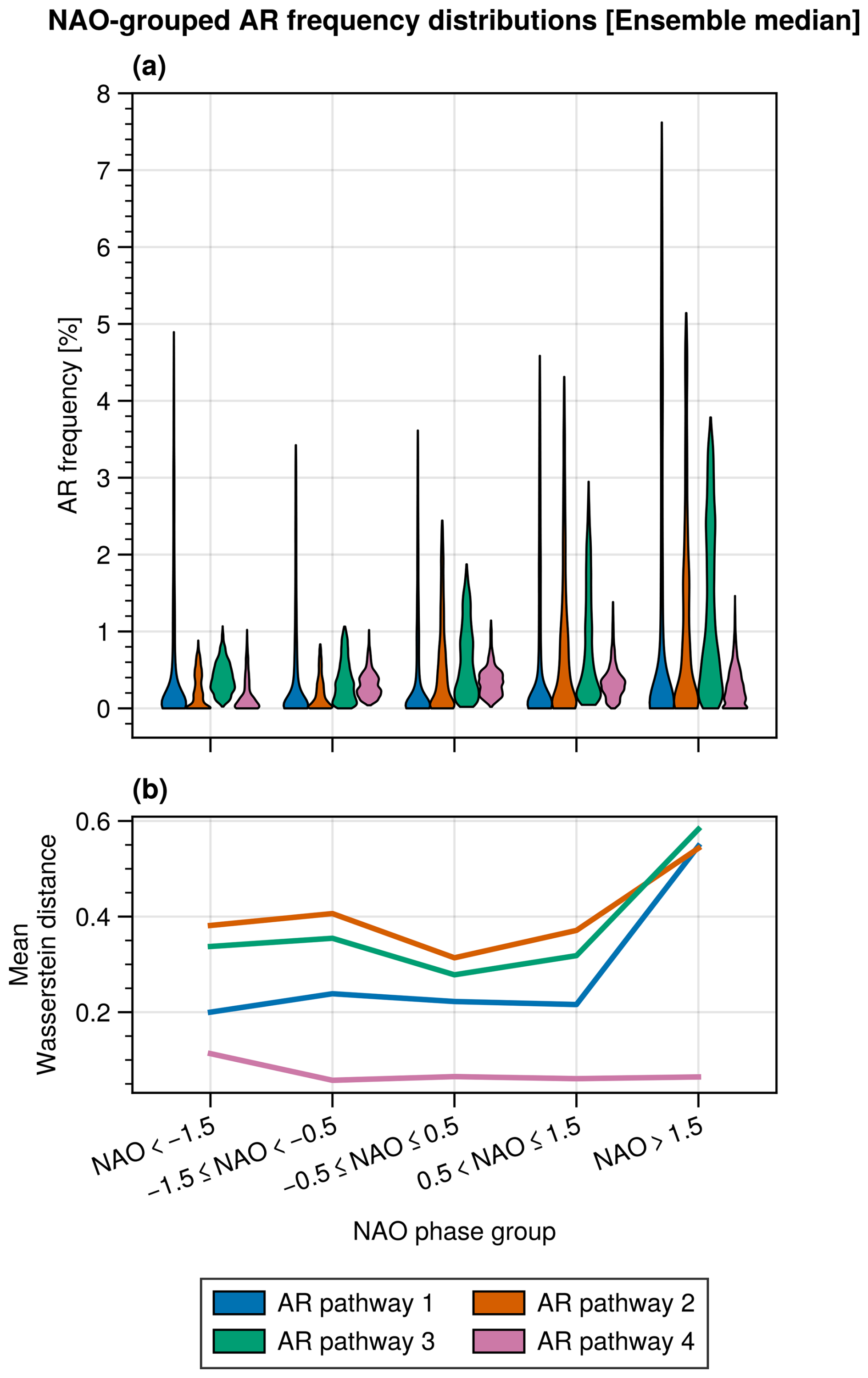
Figure 9 (a) Violin plots showing the distributions of spatial AR frequencies from Fig. 8 (ensemble median), grouped by NAO phase. The height of the violin covers the whole range of values in the distribution, while the width at any given value indicates the relative frequency of that value in the distribution. (b) Mean Wasserstein distance between the successive distributions for each AR pathway.

A majority of the AR activity in pathway 2 takes place during the positive phases of the NAO, where peak AR frequencies exceed 4.0 % [0.5 %–6.7 %] (Figs. 8k–o, A7k–o, A8k–o). Here we note that the maximum AR frequencies nearly doubles between the neutral and positive phases. The frequency difference between the positive and strong positive phase is slightly strengthened in the catalogue ensemble maximum (Fig. A8n, o), where the maximum frequency difference is 1.5 percentage points. Pathway 2 also shows the overall highest mean Wasserstein distance, which indicates that the AR frequencies in pathway 2 change the most with the NAO (Fig. 9a–b).

Similar to pathway 2, ARs in pathway 3 are more frequent during the positive phases of the NAO. Here, AR frequencies reach 2.9 % [0.6 %–8.8 %] during the positive phase of the NAO, while it reaches 3.8 % [1.0 %–12.5 %] during the strong positive phase (Figs. 8s, t, A7s, t, A8s, t). For the strong negative and negative phases of the NAO, frequencies reach 1.1 % [0.1 %–2.7 %] (Figs. 8p, q, A7p, q, A8p, q) over a limited area. For pathway 3 we note that there is a relatively large difference in both the shape and location of the AR frequency pattern between NAO bins. The mean Wasserstein distance for pathway 3 is high, similar to pathway 2 (Fig. 9). Interestingly, in the ensemble maximum (Fig. A10), the mean distances surpasses those of pathway 2.

In pathway 4, during the negative and neutral phases of the NAO, differences in AR activity are relatively small, with frequencies reaching ∼ 1.0 % [0.1 %–1.6 %] (Figs. 8u–w, A7u–w, A8u–w). During the strong positive phase of the NAO, AR frequencies reaches up to 1.5 % [0.3 %–2.2 %] (Figs. 8y, A7y, A8y). These relatively small changes in AR activity with the NAO are also reflected in the mean Wasserstein distance for pathway 4 (Fig. 9).

Overall, comparing the southern ARs in pathway 1 to the more northern-reaching ARs, most notably pathway 2, the northern ARs appear to be more strongly linked to the NAO. This is consistent with previous research, which found that ARs in Northern Europe are more frequent during the positive phase of the NAO (Lavers and Villarini, 2013). A possible explanation for this is that the more southern ARs are primarily governed by the climatological mean flow, whereas the more northerly ARs that make landfall in pathways 2 and 3 are strongly influenced by the enhanced westerlies during positive phases of the NAO.

Regarding the seasonality of the ARs in pathway 2, compared to the seasonality of the Northern Hemisphere storm tracks, where intensity peaks during autumn and winter (e.g., Hoskins and Hodges, 2019), the peak season of these northernmost ARs appears to be shifted slightly more towards the summer months. This suggests a possible different mechanism driving the seasonality of these northern ARs, potentially the higher water content of the warmer summer atmosphere. As we have shown, AR activity is also strongly driven by the NAO, but the seasonal cycle of the NAO does not coincide with the observed seasonal cycle of ARs.

3.5 AR catalogue ensemble spread and uncertainties

The spread in the detected AR frequency within the catalogue ensemble is relatively large. The difference between the members with highest and lowest annual AR frequencies is 9.8 percentage points (Figs. A1a and A2a). Similarly, the ensemble range for the AR-related precipitation fraction is 47.1 percentage points, or ∼ 1200 mm. The large spread is also evident in the field correlation between AR frequency and AR-related precipitation patterns, which ranges from 0.09 and 0.78. This large difference in the AR detection rate, and subsequent AR-related precipitation, among the AR catalogues is largely determined by the IVT thresholds employed by the ARDTs (Rutz et al., 2019). Here we note that the GuanWaliser_v2, Mundhenk_v3, and TempestLR ARDTs employ thresholds that in different ways account for the spatial and seasonal variations in the climatological moisture transport. The GuanWaliser_v2 ARDT achieves this by using a percentile-based threshold that varies with grid point and season. Mundhenk_v3 uses a fixed threshold on IVT anomalies after removing the climatological mean IVT and seasonal cycle at each grid point. The TempestLR ARDT employs a fixed threshold using the Laplacian of the IVT, which identifies ridges where the IVT has increased relative to the climatological IVT (McClenny et al., 2020). These thresholds, which are effectively variable with respect to IVT, allow these ARDTs to detect ARs at higher latitudes, where atmospheric water vapour and IVT are typically lower due to lower air temperatures. In contrast, the Reid500 ARDT, which is designed for lower latitudes, employs a fixed IVT threshold. Specifically, this version uses a fixed threshold of 500 kg m⁻¹ s⁻¹, which will limit its ability to detect ARs in the high latitude region of Scandinavia. Overall, the percentile-based GuanWaliser_v2 algorithm produces the highest AR frequencies, whereas the Mundhenk_v3 and TempestLR ARDTs yield relatively similar results. Interestingly, Mundhenk_v3 and TempestLR show a similar seasonal cycle for the southernmost AR pathway (Figs. 6a, 7a), while the differences are larger in the more northern AR pathway (Figs. 6b, c and 7b, c).

Given the relatively dry atmospheric conditions in the high-latitude region around Scandinavia, ARDTs using variable IVT thresholds are more suitable for identifying ARs in the region, as they account for the climatological background moisture content. Alternatively, lowering the IVT threshold of the Reid500 ARDT would improve its ability to detect ARs over the region, possibly yielding results more aligned with the other ARDTs used in this study. We note that there is a version of the Reid ARDT with a 250 kg m⁻¹ s⁻¹ IVT threshold; however, results from applying this ARDT to ERA5 data have not been published through the ARTMIP project.

We have analysed four different ARDTs applied on a single reanalysis dataset (ERA5). Using multiple reanalysis products would increase the robustness of our results by enabling us to explore the uncertainties introduced by the choice of reanalysis product. However, while there are notable differences in, for instance, the mean IVT in different reanalysis products, the spread in global AR detection due to differences among the ARDTs is overall larger (Collow et al., 2022). Therefore, we considered the use of a single reanalysis dataset to be sufficient for our analysis.

Our method uses tracked ARs to improve the clustering of ARs. Notably, the ARTMIP catalogue does not provide ARDT native tracking data for the ARs. Instead, we have performed our own tracking of the AR objects. It is important to note that we have not implemented the tracking methods specific to each ARDT; instead, we have used an implementation based on the tracking method of the GuanWaliser_v2 ARDT. It is possible that this has introduced some differences compared to the original tracking. However, it was not considered feasible to re-implement four different tracking algorithms for this study. We suggest that incorporating tracking information into the ARTMIP catalogue would be a valuable enhancement.

4 Conclusions

In this study we have presented a climatology of ARs that make landfall in Scandinavia during 1980–2019. The results are based on the output from four different AR detection algorithms from the ARTMIP project, which were applied to ERA5 reanalysis data. The values presented in this section represent the median from analyses conducted on these four AR catalogues. In connection to generating the AR climatology, we have used ERA5 precipitation to evaluate how Scandinavian ARs affect the regional precipitation.

We found that ARs are a regular feature of the Scandinavian climate, with a considerable impact on the regional precipitation. Looking at the entire region, AR activity peaks over Denmark, where the average annual AR frequencies reach 5.9 % of the time, corresponding to around 22 AR days per year. These areas of relatively high AR frequencies extend both west towards the southwest coast of Sweden, and north towards the southwest coast of Norway, and show only slightly lower annual AR frequencies between 3.6 % and 4.8 %. For the entirety of Scandinavia, ARs that intersect the region are present for 25 % of the time during the average year.

The corresponding spatial average AR-related precipitation is 200 mm, or 20 % of the annual total. Notably, the AR-related precipitation is focused along the mountainous coast of Norway, where it makes up 40.7 % of the annual total, most likely due to orographic uplift. However, even far inland across Norway, Sweden, and Denmark, AR-related precipitation still constitutes a substantial fraction (> 24 %) of the annual total precipitation.

We identified four frequent pathways of ARs that reach and intersect Scandinavia: (1) ARs from southwest reaching southern Denmark; (2) ARs from the southwest reaching the northern west coast of Norway; (3) ARs from the west reaching southern Norway and the west coast, and further inland across to the east coast, of Sweden; and (4) ARs from the south reaching the southwest coast of Norway. Out of these four pathways, the ARs reaching southern Denmark are the most frequent, followed by the ARs reaching northern Norway. The spatial maximum AR-related precipitation values for the four pathways correspond to 19.7 %, 13.1 %, 15.1 %, and 7.8 % of total annual precipitation, respectively. The four pathways share a similar seasonal cycle, with AR activity generally peaking during autumn and reaching a minimum during spring, with no significant long-term trends during the study period.

Scandinavian ARs show a strong positive connection to the North Atlantic Oscillation. For all four AR pathways, the AR activity peaks during the strong positive phase of the NAO (> 1.5). Notably, this relationship varies spatially: the northernmost ARs exhibit a more linear relationship with the NAO index, while the southern ARs show high AR frequencies during both the strong negative and strong positive NAO phase.

Our analysis reveals that there are large differences among the four AR catalogues. For the annual AR frequency, the difference between the AR catalogues with the lowest and highest AR activity is around 10 percentage points, while the maximum AR-related precipitation fraction varies between 10 % and 57 %. These differences are largely explained by whether the ARDT employs a fixed or a variable IVT threshold, with ARDTs using variable thresholds yielding higher AR activity. However, there are also noticeable differences within this group, where the annual AR frequency varies by around 5 percentage points. This large spread underscores the importance of evaluating multiple detection algorithms in AR studies.

The significant role of ARs on precipitation over Scandinavian, as shown here, raises the question of whether diagnosing and tracking ARs in numerical weather prediction could improve the accuracy of local precipitation forecasts. Although such approaches have been evaluated for other regions in the world (e.g., Wick et al., 2013; Nayak et al., 2014), dedicated implementation efforts would be needed for Scandinavia. Additionally, distinguishing the contributions of ARs to rainfall versus snowfall would provide valuable insights into their influence on Scandinavia's hydrological cycle. Looking ahead, understanding how the frequency and climate impacts of Scandinavian ARs will change throughout the 21st century represents a crucial next step for understanding regional climate change in Northern Europe.

Appendix A: Figures

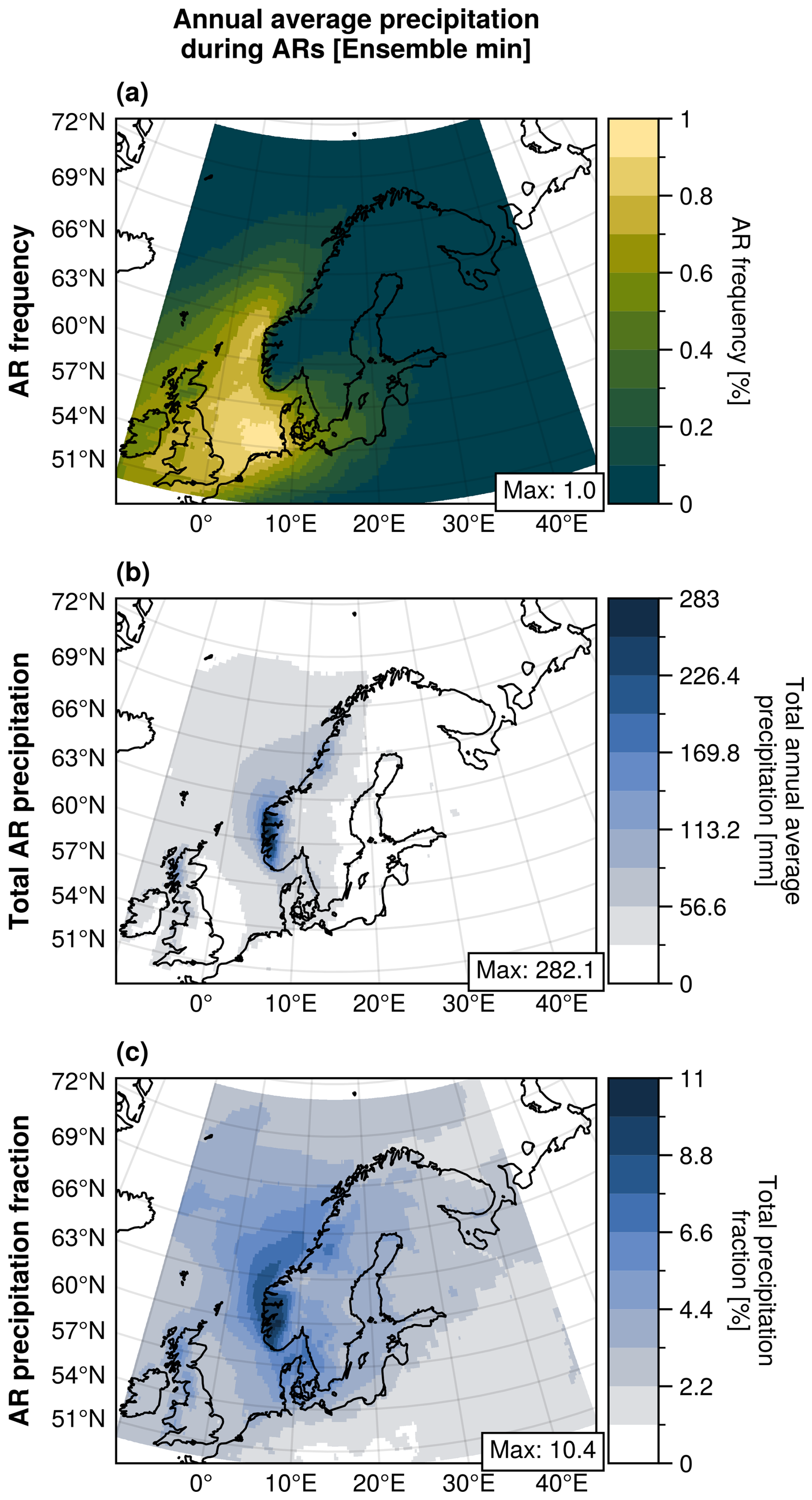
Figure A1 (a) Annual average AR frequency, (b) annual total AR-related precipitation, and (c) fraction of total precipitation attributed to ARs over Scandinavia between 1980 and 2019. All values represent the minimum of the catalogue ensemble, which comprises four AR detection algorithms: Mundhenk_v3, GuanWaliser_v2, Reid500, and TempestLR. Both the AR frequency and precipitation aggregates are based on ERA5 reanalysis data.

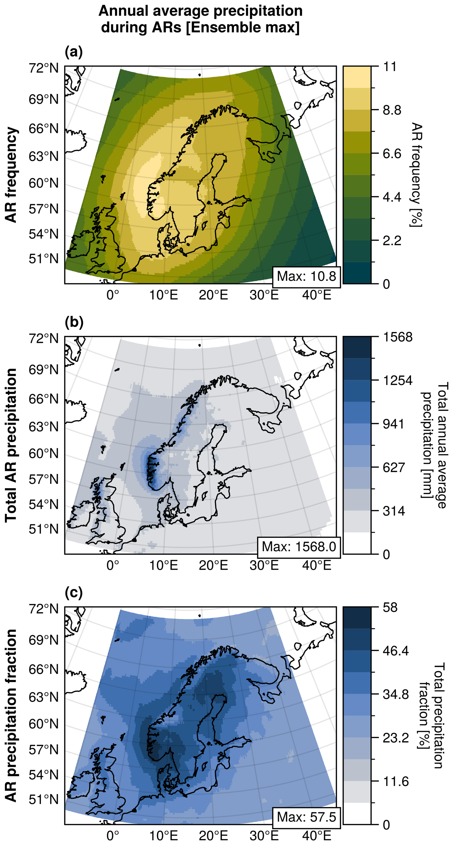
Figure A2 (a) Annual average AR frequency, (b) annual total AR-related precipitation, and (c) fraction of total precipitation attributed to ARs over Scandinavia between 1980 and 2019. All values represent the maximum of the catalogue ensemble, which comprises four AR detection algorithms: Mundhenk_v3, GuanWaliser_v2, Reid500, and TempestLR. Both the AR frequency and precipitation aggregates are based on ERA5 reanalysis data.

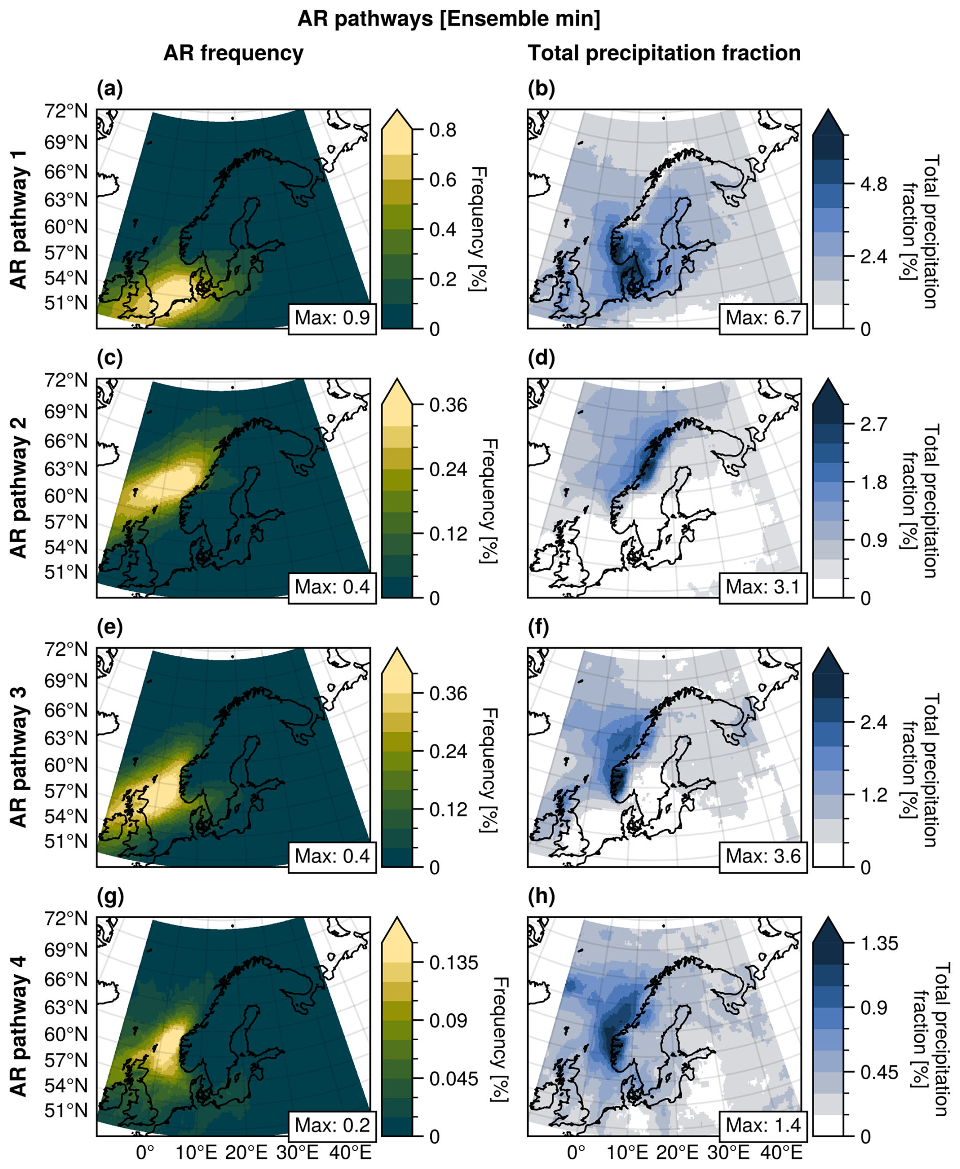
Figure A3 Ensemble minimum annual average AR frequencies (a, c, e, g) and total precipitation fraction (b, d, f, h) for each identified AR pathway (rows). Note that the colour scales differ between the subplots.

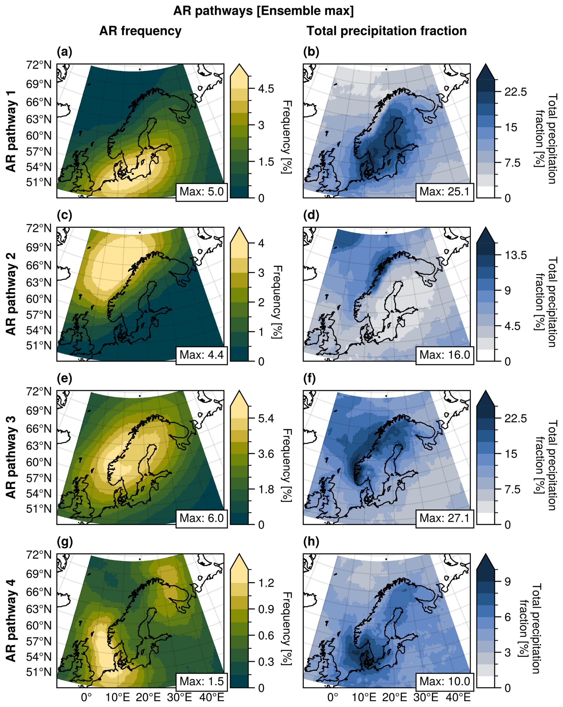
Figure A4 Ensemble maximum annual average AR frequencies (a, c, e, g) and total precipitation fraction (b, d, f, h) for each identified AR pathway (rows). Note that the colour scales differ between the subplots.

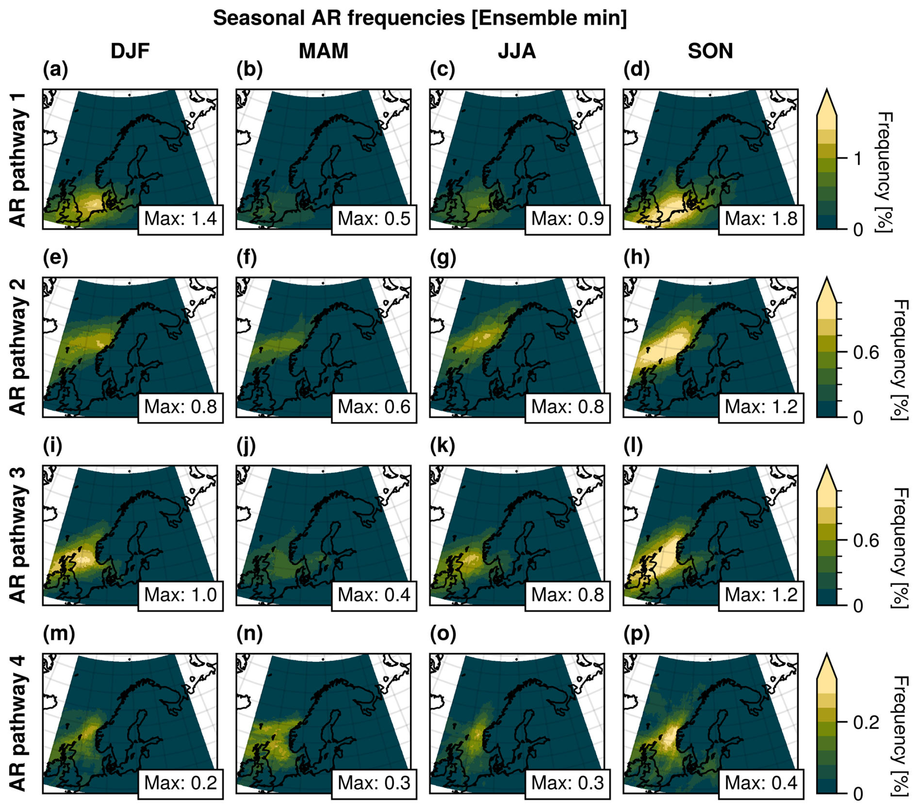
Figure A5 Maps of the average annual AR frequencies (ensemble minimum) during the seasons: winter (DJF), spring (MAM), summer (JJA), and autumn (SON) for each AR pathway. The frequencies correspond to the fraction of AR time steps relative to the total number of time steps within each season. Note that the colour scales differ between AR pathways (rows).

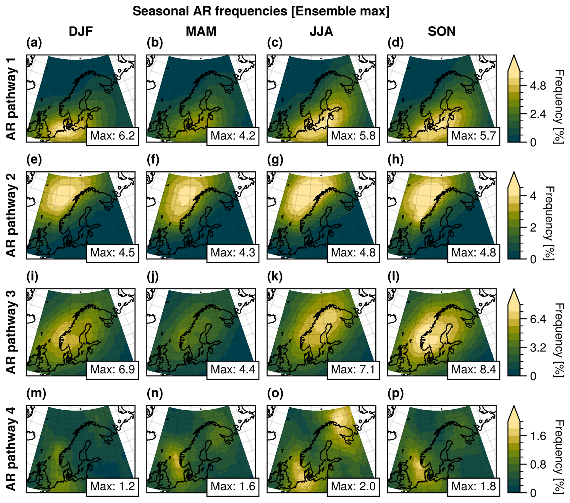
Figure A6 Maps of the average annual AR frequencies (ensemble maximum) during the seasons: winter (DJF), spring (MAM), summer (JJA), and autumn (SON) for each AR pathway. The frequencies correspond to the fraction of AR time steps relative to the total number of time steps within each season. Note that the colour scales differ between AR pathways (rows).

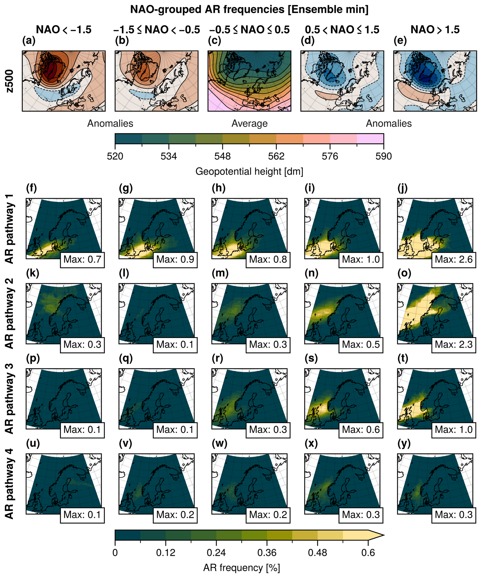
Figure A7 (a–e) Maps of 500 hPa geopotential height over the North Atlantic region during the different phases of the North Atlantic Oscillation (NAO). Panel (c) displays the mean geopotential height during the neutral phase. Panels (a), (b), (d), and (e) show geopotential height anomalies relative to the neutral phase, with contours every 5 dm starting at ±2 dm. Positive anomalies are shown with solid lines and red shading, while negative anomalies are shown with dashed lines and blue shading. (f–y) Corresponding AR frequencies (ensemble minimum) over Scandinavia for each AR pathway and NAO phase. Note that the colour scale of the AR frequency is capped at 0.6 %, with the maximum frequency value for each subplot is displayed in the bottom-right corner.

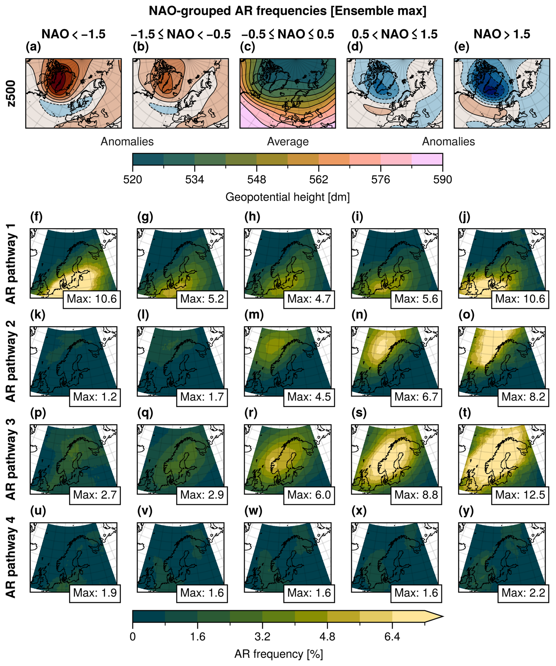
Figure A8 (a–e) Maps of 500 hPa geopotential height over the North Atlantic region during the different phases of the North Atlantic Oscillation (NAO). Panel (c) displays the mean geopotential height during the neutral phase. Panels (a), (b), (d), and (e) show geopotential height anomalies relative to the neutral phase, with contours every 5 dm starting at ±2 dm. Positive anomalies are shown with solid lines and red shading, while negative anomalies are shown with dashed lines and blue shading. (f–y) Corresponding AR frequencies (ensemble maximum) over Scandinavia for each AR pathway and NAO phase. Note that the colour scale of the AR frequency is capped at 7.2 %, with the maximum frequency value for each subplot is displayed in the bottom-right corner.

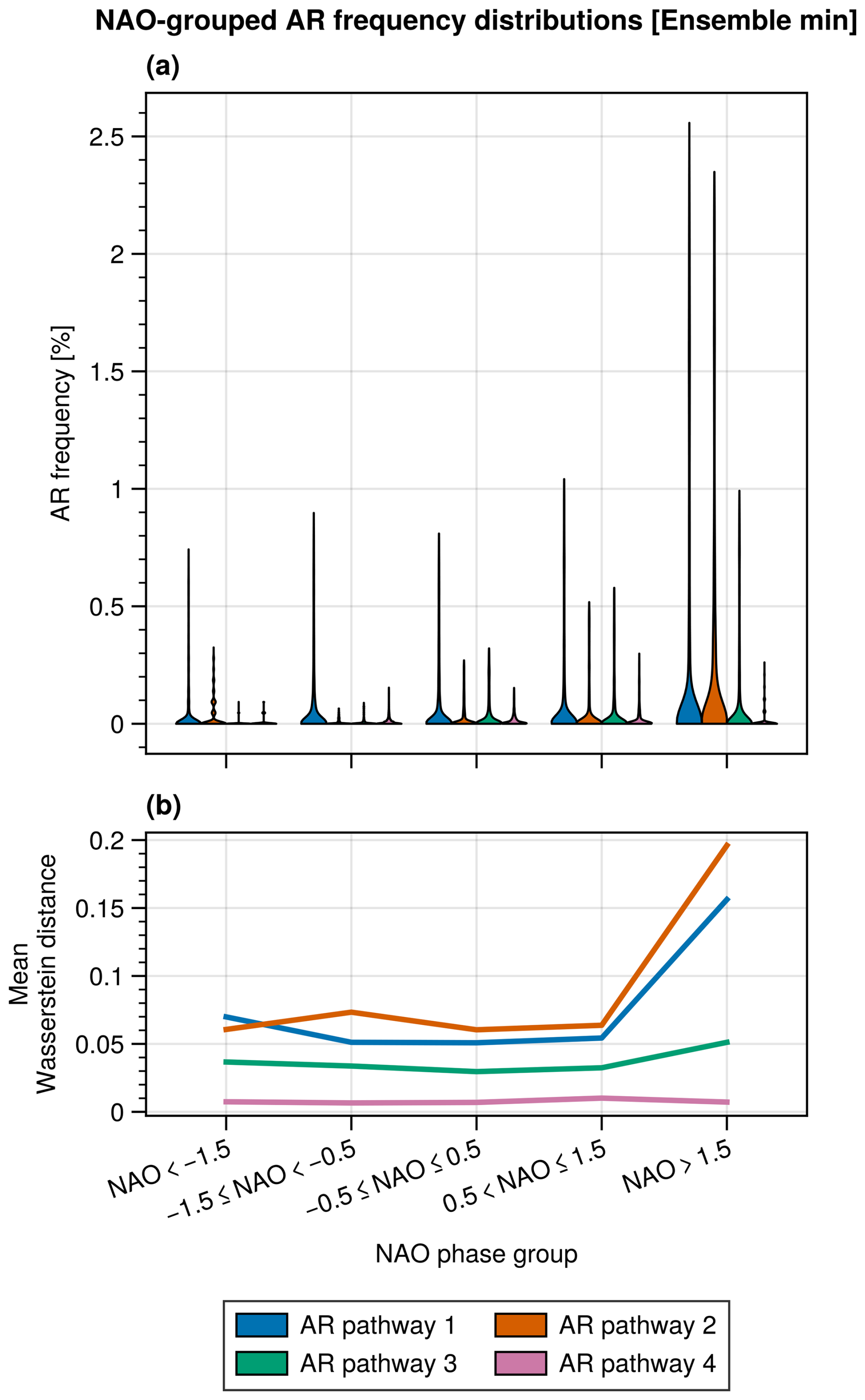
Figure A9 (a) Violin plots showing the distributions of spatial AR frequencies from Fig. A7 (ensemble minimum), grouped by NAO phase. The height of the violin covers the whole range of values in the distribution, while the width at any given value indicates the relative frequency of that value in the distribution. (b) Mean Wasserstein distance between the successive distributions for each AR pathway.

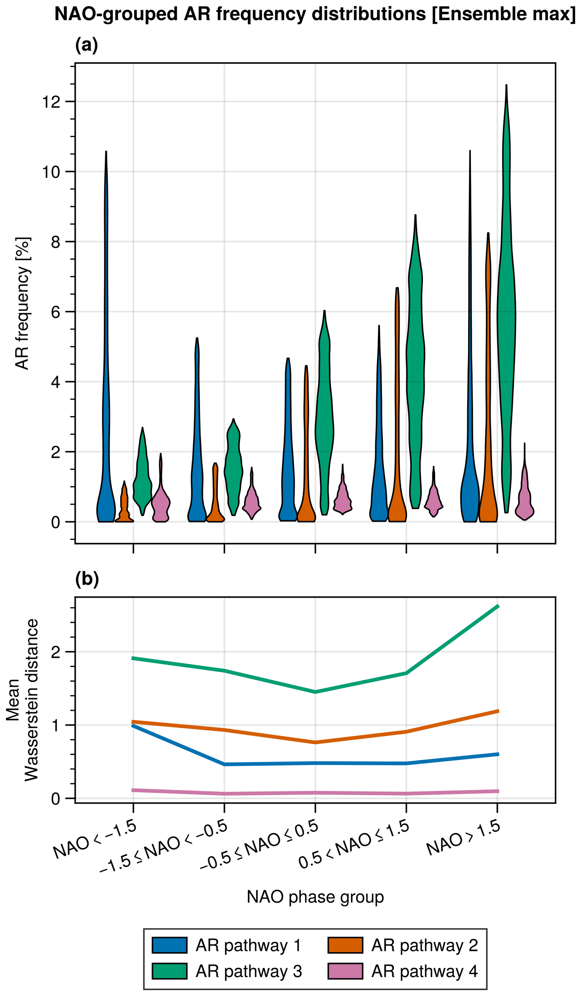
Figure A10 (a) Violin plots showing the distributions of spatial AR frequencies from Fig. A8 (ensemble maximum), grouped by NAO phase. The height of the violin covers the whole range of values in the distribution, while the width at any given value indicates the relative frequency of that value in the distribution. (b) Mean Wasserstein distance between the successive distributions for each AR pathway.

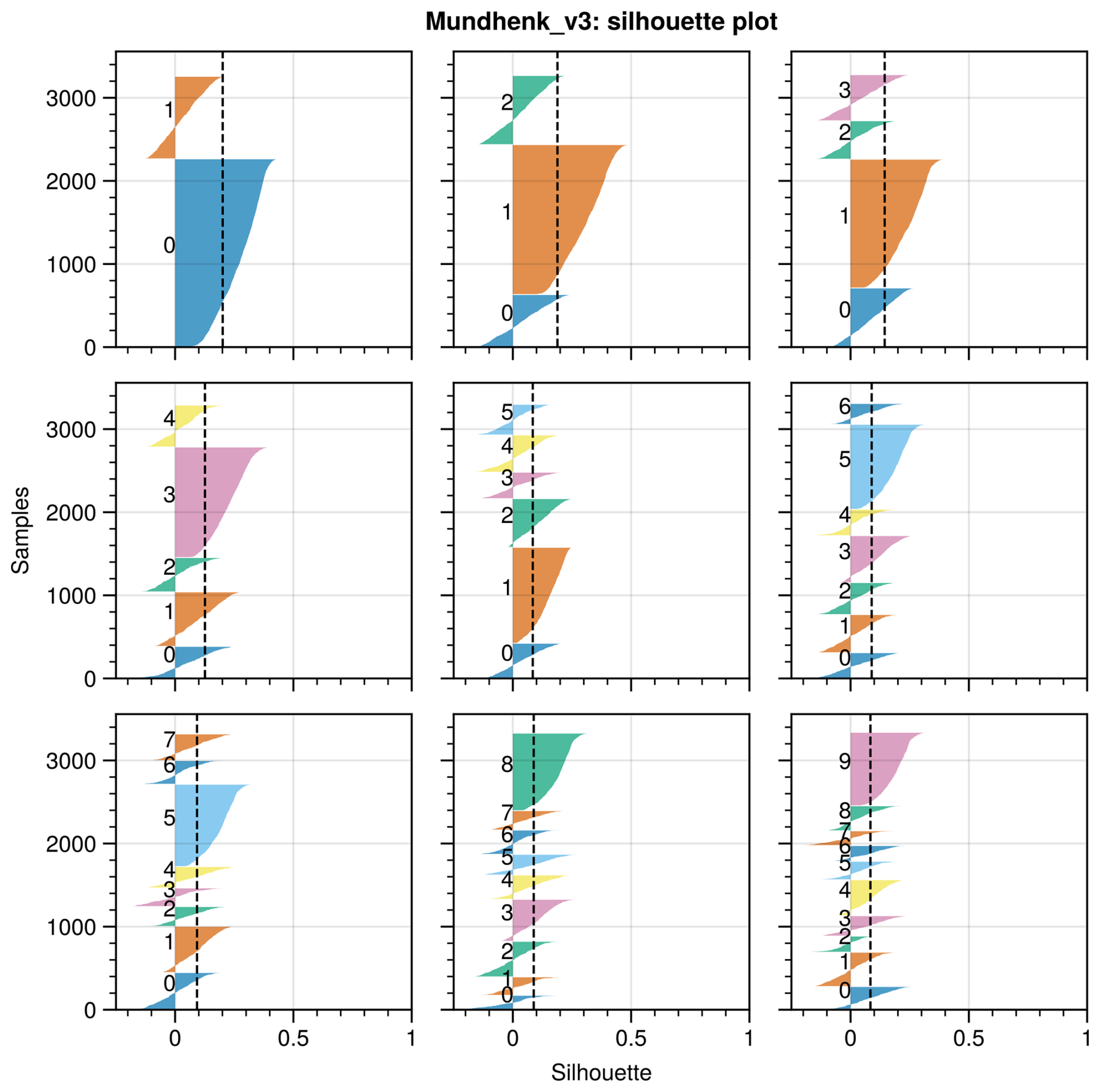
Figure A11 Silhouette plots for the Mundhenk_v3 ARDT. Each panel holds the silhouette for the respective number of clusters.

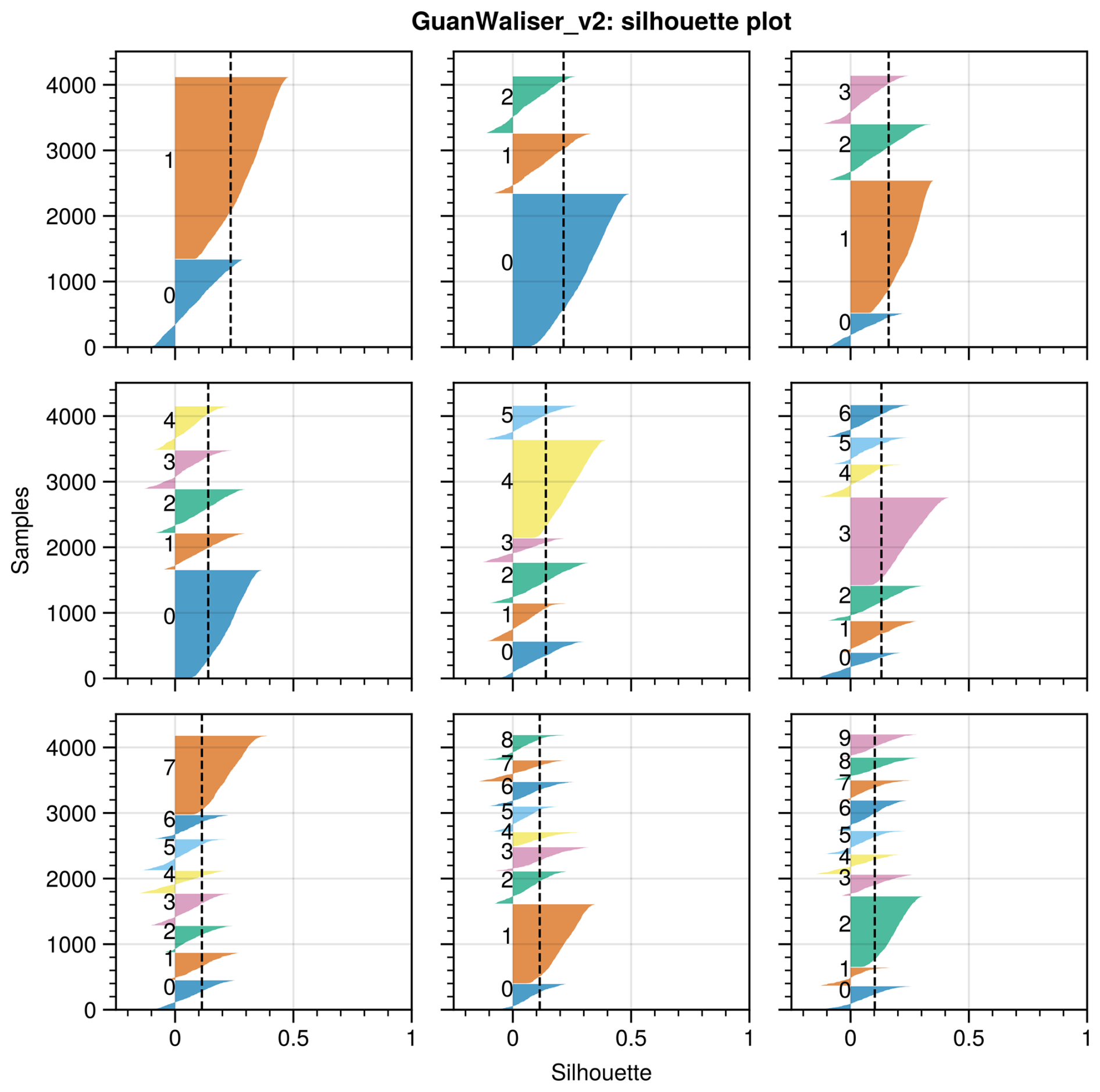
Figure A12 Silhouette plots for the GuanWaliser_v2 ARDT. Each panel holds the silhouette for the respective number of clusters.

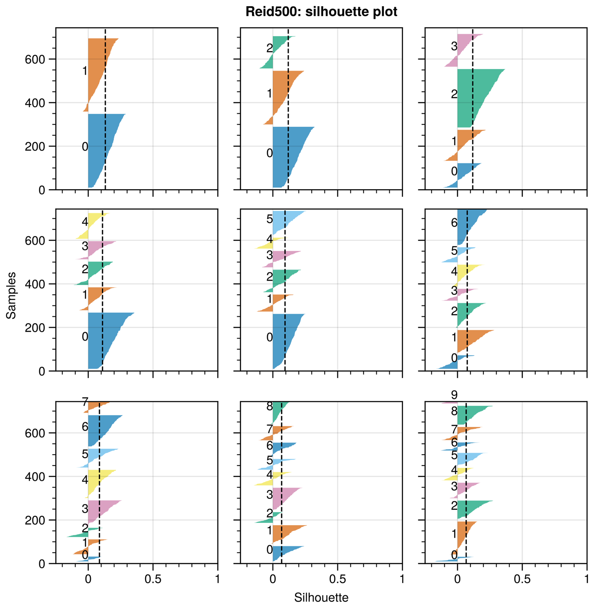
Figure A13 Silhouette plots for the Reid500 ARDT. Each panel holds the silhouette for the respective number of clusters.

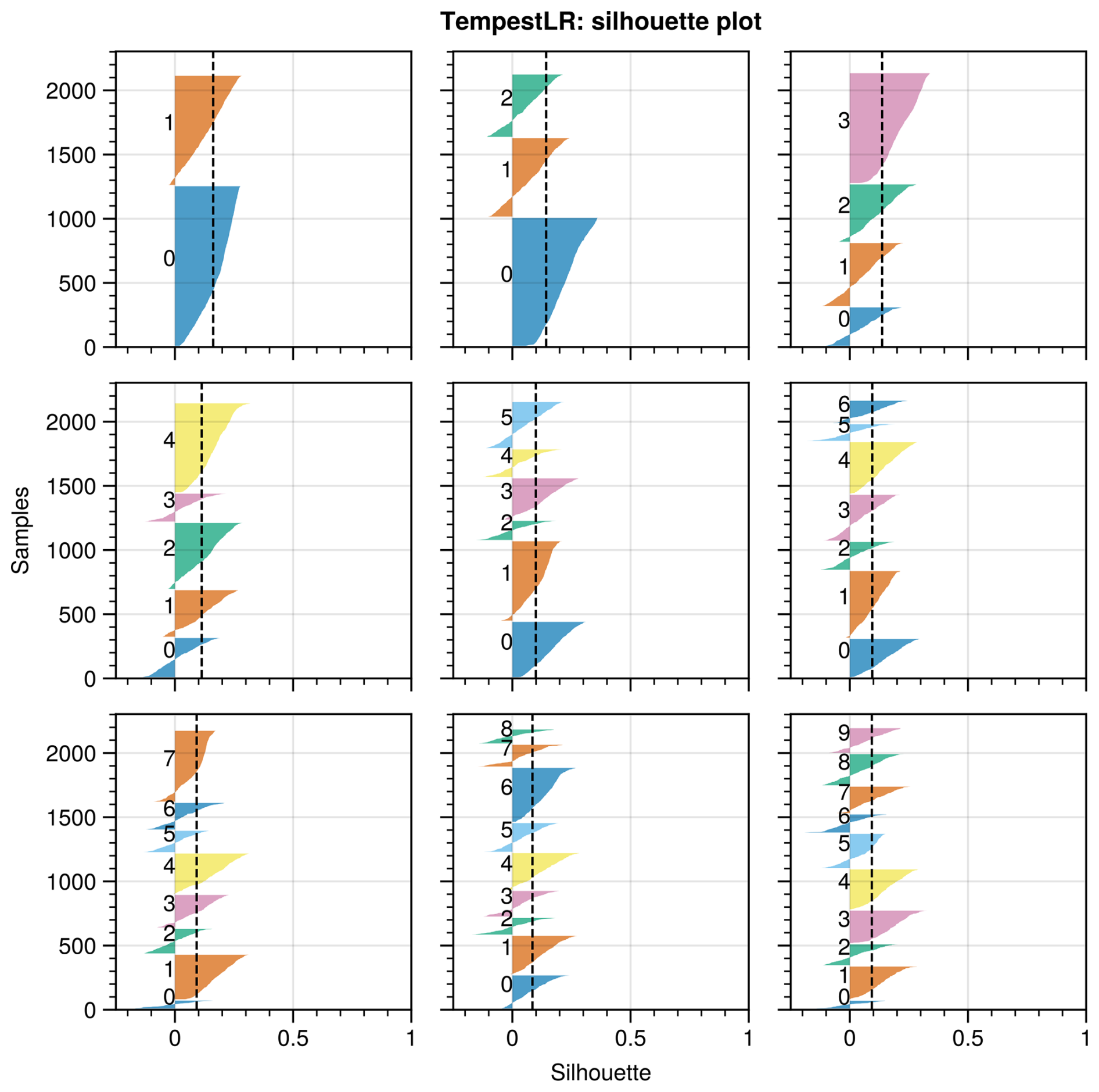
Figure A14 Silhouette plots for the TempestLR ARDT. Each panel holds the silhouette for the respective number of clusters.