Synoptic perspective on the conversion and maintenance of local available potential energy in extratropical cyclones

Extratropical cyclones are the predominant weather system in the midlatitudes. They intensify through baroclinic instability, a process in which available potential energy (APE) is converted into kinetic energy (KE). While the planetary-scale conversion of APE to KE is well understood as a mechanism for maintaining the general atmospheric circulation against dissipation, the synoptic-scale perspective on this conversion is less explored. In this study, we analyze the three-dimensional distribution of APE and the physical processes that consume APE for an illustrative case study and a climatology of 285 intense North Atlantic extratropical cyclones in the winters of 1979–2021 using the ERA5 reanalysis. We utilize a recently introduced local APE framework that allows for APE to be quantified at the level of individual air parcels. The geographical APE distribution is shown to be controlled by the large-scale upper-level circulation. Cyclones draw energy from the upper-tropospheric polar APE reservoir along with the development of the associated upper-level trough. This upper-level APE is converted into KE by air descending along the trough's western flank and acts as the incipient cyclone's primary source of KE. Conversely, KE is converted back into APE during the ascent ahead of the trough, reflecting the deceleration of air parcels as they exit the cyclone region. The diabatic dissipation of APE due to surface sensible heat fluxes along the Gulf Stream front is small compared to the adiabatic conversion of APE to KE, since most of the APE is concentrated and consumed in the middle to upper troposphere and cannot be exposed to surface diabatic forcing. In conclusion, by employing a local APE framework, this study provides a detailed investigation of the synoptic dynamics linking extratropical cyclones and planetary-scale energetics.

1 Introduction

The global atmospheric circulation in midlatitudes is maintained against friction by the conversion of available potential energy (APE) to kinetic energy (KE). Margules (1903) recognized that only a minor fraction of the total potential energy of the atmosphere can be converted to KE by an adiabatic redistribution of mass. This fraction of the total potential energy later became known as APE. In his seminal work, Lorenz (1955) defined APE as the difference between the total potential energy of the atmosphere and the minimum potential energy attainable by an adiabatic rearrangement, a state he referred to as the reference state. This hypothetical reference state represents an atmosphere in mechanical equilibrium, where the highest-density air is at the bottom and the lowest-density air is at the top of the atmosphere such that no meridional density gradients exist. A deviation in the mass distribution from the reference state indicates the availability of potential energy that can be converted into KE through the sinking of high-density air and the rising of low-density air.

The dominant physical mechanism for the conversion of APE to KE in midlatitudes is given by baroclinic instability (Charney, 1947; Eady, 1949), which leads to an equatorward and downward movement of cold air, as well as a poleward and upward movement of warm air within intensifying midlatitude baroclinic waves and thus in particular in extratropical cyclones (Browning and Roberts, 1994). Within the global APE budget, this baroclinic conversion results in the consumption of APE because it brings the atmosphere closer to its hypothetical reference state. The restoration of APE is achieved through the differential heating of the atmosphere by the solar irradiance (Oort, 1964; Peixóto and Oort, 1974).

The Lorenz APE is defined as a volume integral of a closed system, which is why previous studies have largely focused on the global integral of APE. Bosart et al. (1996) pointed to the significance of individual synoptic-scale weather systems for the planetary-scale APE reservoir. They demonstrated that the development of a single explosive extratropical cyclone over North America was concurrent with a 10 % drop in Northern Hemisphere APE. Further studies have underscored the relevance of synoptic-scale dynamics for the variability in APE (Wintels and Gyakum, 2000; Bowley et al., 2019). However, the volume-integrated formulation of Lorenz APE limits its applicability on synoptic scales. A decomposition into eddy and mean components allows for the attribution of volume-integrated APE conversion to synoptic-scale dynamics (Lorenz, 1955; Peixóto and Oort, 1974), but it remains challenging to attribute such time-filtered quantities to individual weather systems. The Lorenz APE can be localized by selecting a local domain, such as a box around a cyclone, within which the reference state is calculated (Smith, 1969, 1980; Johnson, 1970; Gertler et al., 2023). However, a local reference state makes it difficult to quantify the advection of APE into and out of the local domain. Moreover, a cyclone does not represent a closed system, complicating the interpretation of energy exchange between the local and the global domain. In fact, as we will show here, the advection of high-APE air into the environment of the extratropical cyclones is a key component in their energy budgets.

The presence of APE implies a baroclinic atmosphere, and baroclinicity is straightforward to define locally (Eady, 1949; Papritz et al., 2015). Therefore, past studies have often resorted to baroclinicity as a local measure for the potential of cyclone development (Ambaum and Novak, 2014; Novak et al., 2017). However, baroclinicity measures the maximum growth rate of a baroclinic disturbance, not the potential for baroclinic growth (Eady, 1949).

To describe APE conversion within weather systems, it is necessary to employ a truly local APE framework. Holliday and McIntyre (1981) and Andrews (1981) introduced local frameworks that describe APE as a local energy density for a compressible nonhydrostatic fluid and an incompressible fluid, respectively. Subsequently, Novak and Tailleux (2018) extended this framework to the dry hydrostatic primitive equations and demonstrated that the global integral of this local APE density is equivalent to the Lorenz APE.

The climatological analysis of Novak and Tailleux (2018) reveals spatial characteristics of APE and its conversion, which were previously discussed only as global integrals (Oort, 1964; Peixóto and Oort, 1974). In particular, they find that APE is mainly located in the polar middle and upper troposphere, where the air is colder than its reference state. They also showed that APE is advected from this polar reservoir into the storm tracks. There eddy APE is converted to eddy KE by adiabatic processes, while diabatic processes create eddy APE. Since their analysis was climatological, many questions remain regarding the synoptic environment leading to the advection of APE into the storm tracks, the physical processes giving rise to adiabatic and diabatic tendencies of APE, and their link to baroclinic wave activity in the storm tracks.

In their analysis of local APE within an idealized baroclinic channel simulation, Federer et al. (2024) employed Lagrangian trajectories to demonstrate how APE is advected into the baroclinic zone along the upper-level trough in the cold sector of a surface cyclone. Their findings revealed that locally, within a baroclinic wave, substantial amounts of APE are not only consumed but also produced. This is consistent with a local notion of APE, where air parcels not only accelerate the flow by converting APE to KE but also decelerate it by converting KE back to APE. The volume-integrated net conversion then informs about the intensification or the decay of the baroclinic wave in terms of its KE. However, important differences exist between the highly idealized baroclinic channel and the real atmosphere.

First of all, the reference state based on an adiabatic rearrangement of the real atmosphere differs from the reference state computed from a symmetric baroclinic channel due to the spherical geometry of Earth. In the baroclinic channel, there is approximately the same amount of APE on the equatorward and the poleward side of the baroclinic zone (Federer et al., 2024). In contrast, the mass of air equatorward of the midlatitude baroclinic zone on Earth is much greater than on the poleward side, which implies that the local APE density is larger near the poles than near the Equator (Novak and Tailleux, 2018). Consequently, we anticipate that APE conversion in the real atmosphere will differ from that observed in a baroclinic channel. Second, the baroclinic channel does not include topography, land–sea contrasts, or surface fluxes, which we expect to significantly influence the distribution and conversion of APE (Brayshaw et al., 2009, 2011; Molteni et al., 2011; Portal et al., 2022).

In particular, the Northern Hemisphere storm tracks are significantly influenced by strong sea-surface temperature (SST) fronts along the western boundary currents. The intense heat transfer from the ocean to the atmosphere in these regions (Kwon et al., 2010; Czaja et al., 2019) is known to affect the large-scale circulation (Omrani et al., 2019; Mathews and Czaja, 2024; Wenta et al., 2024). On the one hand, latent heat release following moisture uptake along the Gulf Stream SST front (Pfahl et al., 2014) is known to invigorate cyclone development (Davis and Emanuel, 1991; Dacre and Gray, 2013; Binder et al., 2016) and can contribute to downstream ridge building (Yamamoto et al., 2021; Wenta et al., 2024). On the other hand, it is generally believed that SST fronts anchor midlatitude storm tracks through a process called oceanic baroclinic adjustment (Nakamura et al., 2008; Hotta and Nakamura, 2011). Essentially, the SST front dampens local atmospheric temperature anomalies induced by the meridional advection within developing cyclones, thereby maintaining low-level baroclinicity. A number of studies have indicated that this process results in the dissipation of APE, dampening the development of baroclinic waves (Swanson and Pierrehumbert, 1997; Marcheggiani and Ambaum, 2020). In contrast, strong surface sensible heat fluxes that occur in marine cold-air outbreaks (CAOs) following cyclones have been linked to the maintenance of low-level baroclinicity by reducing static stability (Hotta and Nakamura, 2011; Papritz and Spengler, 2015), which amplifies baroclinic growth rates. This points towards an ambiguous role of sensible and latent heat fluxes along the North Atlantic storm track in the local APE budget. Moreover, it remains unclear how much of the diabatic APE tendency in the storm tracks, as described by Novak and Tailleux (2018), can be attributed to air–sea heat fluxes.

The objective of this study is to gain a comprehensive three-dimensional understanding of the distribution and conversion of local APE along the North Atlantic storm track through both adiabatic and diabatic processes and to elucidate the relationship between local APE and the development of extratropical cyclones. In particular, we will focus on Gulf Stream cyclones in order to investigate the relevance of air–sea interaction on the local APE budget, which potentially has implications for the downstream storm track evolution (Wenta et al., 2024). To this end, we address the following specific questions:

• What determines the distribution and conversion of local APE on synoptic scales over the North Atlantic?

• How does the development of Gulf Stream cyclones influence the distribution and conversion of local APE?

• What is the role of air–sea interaction in the Gulf Stream region in the local APE budget?

The study is structured as follows. In Sect. 2, we will introduce the dataset, the identification and tracking of cyclones, and the local APE framework. Then in Sect. 3, we present a case study of a well-studied rapidly intensifying cyclone in the Gulf Stream region (e.g., Wenta et al., 2024). In Sect. 4, we extend our understanding of the case study to a set of 285 deep Gulf Stream cyclones. Finally, the study concludes with a discussion in Sect. 5.

2 Data and methodology

2.1 Dataset

This study uses the ERA5 reanalysis dataset provided by the European Centre for Medium-Range Weather Forecasts (ECMWF; Hersbach et al., 2020). We utilize data on model levels interpolated to a 0.5°×0.5° longitude–latitude grid at hourly resolution. Our analysis spans 41 winter seasons (DJF, December–January–February) between 1979 and 2021, encompassing data from 1 December 1979 to 28 February 2021.

The pressure at the boundary layer top is diagnosed from the boundary layer height provided by ERA5. In addition, we compute quasi-geostrophic ω (QGω) by inverting the QGω equation following Besson et al. (2021). For this study we only consider QGω forcing at 500 hPa from upper levels.

For studying local APE conversions in cyclones, we objectively identify and track cyclones based on the sea-level pressure (SLP) field using the contour search algorithm developed by Wernli and Schwierz (2006) and refined by Sprenger et al. (2017). Each cyclone is characterized by a pressure minimum, which is tracked over time to generate cyclone tracks, along with an outermost closed contour in the SLP field. The difference between this outermost closed contour and the pressure minimum defines the cyclone's depth, serving as a measure of its intensity. Furthermore, we compute the intensification rate of a cyclone at a given time step by evaluating its pressure change over a 24 h period centered on that time step. As an additional weather feature, we also identify CAOs following the definition by Papritz et al. (2015). Individual CAO grid points are identified using the criterion ${\mathit{\theta }}_{\mathrm{SST}}-{\mathit{\theta }}_{\mathrm{850}}>\mathrm{8}$ K, where θ_SST is the potential sea-surface temperature and θ₈₅₀ is the potential temperature at 850 hPa.

Additionally, we use the Lagrangian Analysis Tool (LAGRANTO; Wernli and Davies, 1997; Sprenger and Wernli, 2015) to compute kinematic backward and forward trajectories. The integration of APE changes along trajectories has proven to be a valuable technique for relating the movement of air parcels to changes in the APE distribution (Federer et al., 2024).

2.2 Local APE framework

In this study we use the local APE framework for a dry hydrostatic atmosphere developed by Novak and Tailleux (2018). Here, we present a brief overview of the most relevant features of this framework. For a detailed introduction into the use of local APE on synoptic scales, we refer to Federer et al. (2024).

The local APE density of an air parcel is defined as

$$\begin{array}{}\text{(1)}& E_{\mathrm{a}}(\mathit{\theta },p,t)=\underset{p_{\mathrm{r}}}{\overset{p}{\int }}\left\{\mathit{\alpha }\left(\mathit{\theta },p^{\prime }\right)-\mathit{\alpha }\left[{\mathit{\theta }}_{\mathrm{r}}\left(p^{\prime },t\right),p^{\prime }\right]\right\}\mathrm{d}{p}^{\prime },\end{array}$$

where the APE density (J kg⁻¹) of an air parcel is denoted by E_a and α is the specific volume, given by the reciprocal of the density $\mathit{\alpha }={\mathit{\rho }}^{-\mathrm{1}}$. The integrand of Eq. (1) is the buoyancy force experienced by an air parcel at pressure p^′ within the reference atmosphere, which is given by a vertical profile of potential temperature ${\mathit{\theta }}_{\mathrm{r}}(p^{\prime },t)$. The reference pressure of the air parcel p_r is determined by the level of neutral buoyancy (LNB) equation ${\mathit{\theta }}_{\mathrm{r}}(p_{\mathrm{r}},t)=\mathit{\theta }(p,t)$. Therefore, the buoyancy force experienced by the air parcel is 0 when the parcel's density matches the surrounding air at the reference pressure p_r. The buoyancy force is maximal at the pressure p where the density difference between the air parcel and the reference environment is greatest. Then, Eq. (1) expresses the work needed to move the air parcel, within the reference atmosphere, from its reference pressure p_r to its actual pressure p.

The APE of an air parcel can change by an adiabatic vertical displacement of the air parcel, by diabatic heating or cooling of the air parcel, or by a change in the reference state. Formally, this is expressed by the total derivative of Eq. (1) representing the total change in APE along the parcel's trajectory. This change is given by

$$\begin{array}{}\text{(2)}& {\displaystyle \frac{\mathrm{D}{E}_{\mathrm{a}}}{\mathrm{D}t}}=\underset{\left(\mathrm{I}\right)}{\underbrace{(\mathit{\alpha }-{\mathit{\alpha }}_{\mathrm{r}})\mathit{\omega }}}+\underset{\left(\mathrm{II}\right)}{\underbrace{\left({\displaystyle \frac{T-T_{\mathrm{r}}}{T}}\right)Q}}-\underset{\left(\mathrm{III}\right)}{\underbrace{\underset{p_{\mathrm{r}}}{\overset{p}{\int }}{\displaystyle \frac{\partial {\mathit{\alpha }}_{\mathrm{r}}}{\partial t}}\mathrm{d}{p}^{\prime }}},\end{array}$$

where $\mathit{\omega }=\mathrm{d}p/\mathrm{d}t$ is the vertical pressure velocity, $Q=c_p\mathrm{d}\mathit{\theta }/\mathrm{d}t$ is the diabatic heating rate, and T is the temperature. According to Eq. (2), the adiabatic tendency of APE (I) is given by the product of ω and the buoyancy of the air parcel with respect to the reference state (α−α_r), which we refer to as the adiabatic efficiency. The diabatic tendency (II) is given by the product of Q and the thermal efficiency $(T-T_{\mathrm{r}})/T$. Finally, the third term (III) expresses the APE tendency due to a change in the reference state with time. Consequently, the APE tendency due to adiabatic and diabatic processes depends not only on the magnitude of ω and Q, respectively, but also on the respective efficiency, which quantifies the departure of the air parcel from its reference state. Because the adiabatic (I) and diabatic (II) tendencies of APE are much larger than the tendency due to changes in the reference state (III), in this study, we will focus on the adiabatic and diabatic tendency. The terms (I–III) present sources and sinks to local APE. Therefore, APE is conserved along adiabatic flow only if ω is 0.

2.3 Computation of the reference state

For the computation of the reference state we follow the parcel-sorting method described by Novak and Tailleux (2018). First, the entire atmosphere is partitioned into air parcels. Second, the atmosphere is deconstructed and the air parcels are sorted by ascending potential temperature. Third, the three-dimensional reference state is reconstructed starting from the surface with the potentially coldest air parcels. To achieve this, we calculate the pressure difference between the bottom and top of every air parcel as if its mass were distributed uniformly across the surface of Earth. Stacking all layers from the lowest to highest potential temperature yields the reference state atmosphere. The computation of the reference state is also illustrated schematically in Fig. S1 in the Supplement. In this reference state, the vertical profile of potential temperature θ_r(p,t) decreases monotonically with pressure and is equal for every grid point. Since there are no meridional temperature gradients in the reference state atmosphere, it represents the state of minimum potential energy attainable by an adiabatic rearrangement of the global atmosphere (Lorenz, 1955; Novak and Tailleux, 2018). This procedure is repeated for every hourly time step of ERA5.

To facilitate a comparison of APE between cyclones at different time steps, we apply a temporal smoothing to the instantaneous reference state vertical profiles. First, we compute daily averages, removing the daily cycle. Next, we apply a 31 d running mean, smoothing out day-to-day variations but retaining the seasonality. Lastly, we apply a 9-year running mean to each calendar time step to take into account the effect of global warming on the reference state.

3 Case study

We first illustrate local APE and its tendencies in a case study to gain a detailed understanding of the synoptic processes that govern the evolution of local APE. For this purpose, an episode of European blocking was selected, which is defined according to the definition of the year-round weather regimes of Grams et al. (2017). The event lasted from 20 to 27 February 2019 and was accompanied by record-high temperatures in France, the Netherlands, and the United Kingdom (Young and Galvin, 2020; Leach et al., 2021). We chose this case study because the buildup and maintenance of the block were linked to several strongly intensifying extratropical cyclones that developed off the coast of North America and along the Gulf Stream SST front (Wenta et al., 2024). Such cyclones are expected to export APE from high latitudes to the North Atlantic storm track (Novak and Tailleux, 2018). In this section, we will illustrate how the large-scale circulation is related to the distribution of local APE, where APE is consumed and generated in the vicinity of cyclones, and what physical processes drive local APE tendencies during the case study period. The insights gained in this case study will subsequently be generalized and extended with a climatological analysis of deep Gulf Stream cyclones in Sect. 4.

3.1 Synoptic APE development

3.1.1 Column-integrated APE distribution

Figure 1 gives an overview of the large-scale circulation around the case study period. The upper-level circulation is indicated by the 2 PVU (1 potential vorticity unit, PVU, is equivalent to 10⁻⁶ K m² kg⁻¹ s⁻¹) contour of isentropic Ertel potential vorticity (PV) at 315 K. On 18 February (Fig. 1a) the first primary cyclone (1a) of the case study begins to develop in the Gulf Stream region in a baroclinic zone which lies at the edge of high APE values toward the north. As the cyclone continues to intensify and propagates into the central North Atlantic (Fig. 1b, c), an upper-level trough forms and extends into lower latitudes, while a ridge is established downstream. High APE values are clearly collocated with the trough extending into the North Atlantic. This points to a strong link between the upper-level PV pattern and the distribution of APE. Because the distribution of PV governs the large-scale circulation, APE is likely linked to the large-scale circulation as well, as will be explored in the following sections.

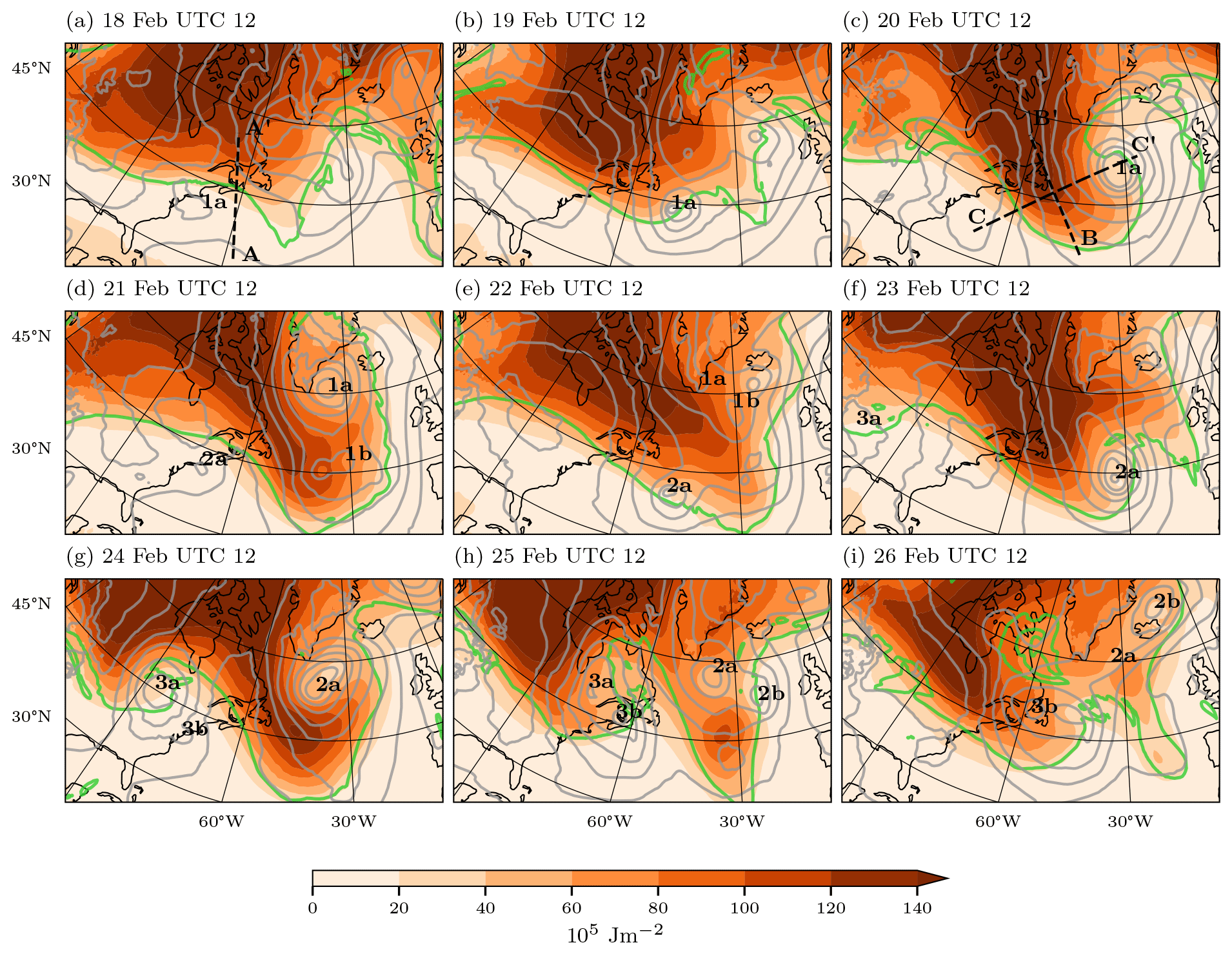
Figure 1 Synoptic overview between 18 February at 12:00 UTC and 26 February at 12:00 UTC at 24 h intervals. Shown are vertically integrated APE between 1050 and 250 hPa (color shading), mean sea-level pressure (grey contours; every 10 hPa), and the 2 PVU contour on the 315 K isentrope (green). Cyclones discussed in the text are labeled (1a, 1b, 2a, 2b, 3a, 3b). The dashed lines in panels (a) and (c) match the cross sections in Fig. 2. The direction of the cross sections is indicated with capital letters at the southern (A, B, C) and northern ends (A^′, B^′, C^′) of the cross section.

As cyclone 1a propagates toward the southern tip of Greenland, a secondary cyclone (1b) develops on the first cyclone's trailing cold front (Fig. 1d) and propagates poleward (Fig. 1e). The development of cyclone 1b also occurs adjacent to high APE values. Concurrently, a second primary cyclone (2a) develops in the Gulf Stream region and follows an evolution very similar to cyclone 1a (Fig. 1d–g). High APE values persist in the central North Atlantic and are again clearly collocated with the upper-level trough. Subsequently, another secondary cyclone (2b) intensifies along the trailing cold front of cyclone 2a. In contrast to cyclone 1b, the high APE values in the central North Atlantic decrease concurrently with the intensification of cyclone 2b. The decline in midlatitude APE is ushered in by the development of cyclones 3a and 3b over continental North America. The advection of low-APE air from the south by this low-pressure system cuts off the APE supply from higher latitudes into the North Atlantic storm track, the quasi-stationary trough–ridge couplet over the North Atlantic decays, and the associated APE is dissipated.

In summary, the case study is characterized by the development of two primary and two secondary North Atlantic cyclones that follow remarkably similar tracks adjacent to regions of high APE values. Those cyclones tap into the reservoir of APE over northeastern Canada and advect APE into midlatitudes. The extension of high-APE air into midlatitudes is collocated with an upper-level trough, which indicates a strong link of the APE distribution to upper-level flow features. The dissipation of APE in the central North Atlantic and the end of intense North Atlantic cyclogenesis are accompanied by the development of an upstream cyclone, which inhibits further APE supply to the North Atlantic.

3.1.2 Vertical structure

The close match between the large-scale circulation and the distribution of vertically integrated APE warrants an investigation of the vertical structure of the APE distribution. Figure 2 shows vertical cross sections of the APE distribution along the dashed lines in Fig. 1. The first cross section (Fig. 2a) shows the APE distribution approximately normal to the baroclinic zone shortly before the development of cyclone 1a. The baroclinic zone is characterized by a strong meridional temperature gradient near the surface and a jet stream aloft, which coincides with a steep tropopause. APE is confined poleward of the baroclinic zone, whereas very little APE is located within the baroclinic zone and equatorward of it. APE also increases with height up to the tropopause and rapidly decreases with height in the stratosphere.

Figure 2 Cross sections as indicated in Fig. 1. Shown are APE (color shading), the 2 PVU contour representing the dynamical tropopause (green), the horizontal wind speed (black contours; every 20 m s⁻¹), and potential temperature (grey contours; every 6 K). For each panel, the position of the cross section is shown in Fig. 1, labeled by capital letters.

Figure 2b shows a meridionally oriented cross section through the trough, which stretches into the central North Atlantic after cyclone 1a intensifies. The vertical distribution of APE across the trough is strongly related to the height of the dynamical tropopause. At the center of the cross section, the tropopause reaches 500 hPa and is accompanied by a local cold anomaly underneath. This local cold anomaly translates to high APE because the air parcels are colder than their reference state. APE located at the southern tip of the trough follows the tropopause, which reaches higher altitudes in the atmosphere compared to the center of the trough. The zonally oriented cross section through the trough (Fig. 2c) further illustrates the cold anomaly below the trough. From left to right the isentropes slope upwards, concurrent with an increase in APE. Thus, the isentropic lifting beneath the upper-level trough is accompanied by high APE values. The APE located in this region is bounded by a jet stream toward the west and cyclone 1a toward the east.

The vertical distribution of APE shows that APE is concentrated in the middle and upper troposphere north of the midlatitude baroclinic zone. The upward bending of isentropes by the positive PV anomaly implies a dome of cold air beneath the trough, which in turn is associated with high APE since the air is colder than its reference state. In summary, the close link between upper-level PV and high-APE air beneath points to the key role of the PV distribution in determining the distribution of APE.

3.2 Adiabatic and diabatic APE modification within the free troposphere

3.2.1 Instantaneous APE tendency

Given that APE is concentrated in the upper troposphere, adjacent to the developing cyclones, the question arises as to how the cyclones tap into the APE reservoir and how the midlatitude APE reservoir is maintained throughout the case study period. First, we consider the instantaneous APE tendency at a single time step (Fig. 3). In midlatitudes, APE is consumed in the wake of cyclone 1a, whereas APE production is focused at the center of the cyclone (Fig. 3a). The net APE tendency is largely adiabatic (Fig. 3b), which means that vertical motion is the main mechanism of APE consumption and production. In contrast, the diabatic tendency almost only consumes APE at the center of the cyclone (Fig. 3c). Therefore, the diabatic tendency partially compensates for APE production by vertical motion at the center of cyclone 1a.

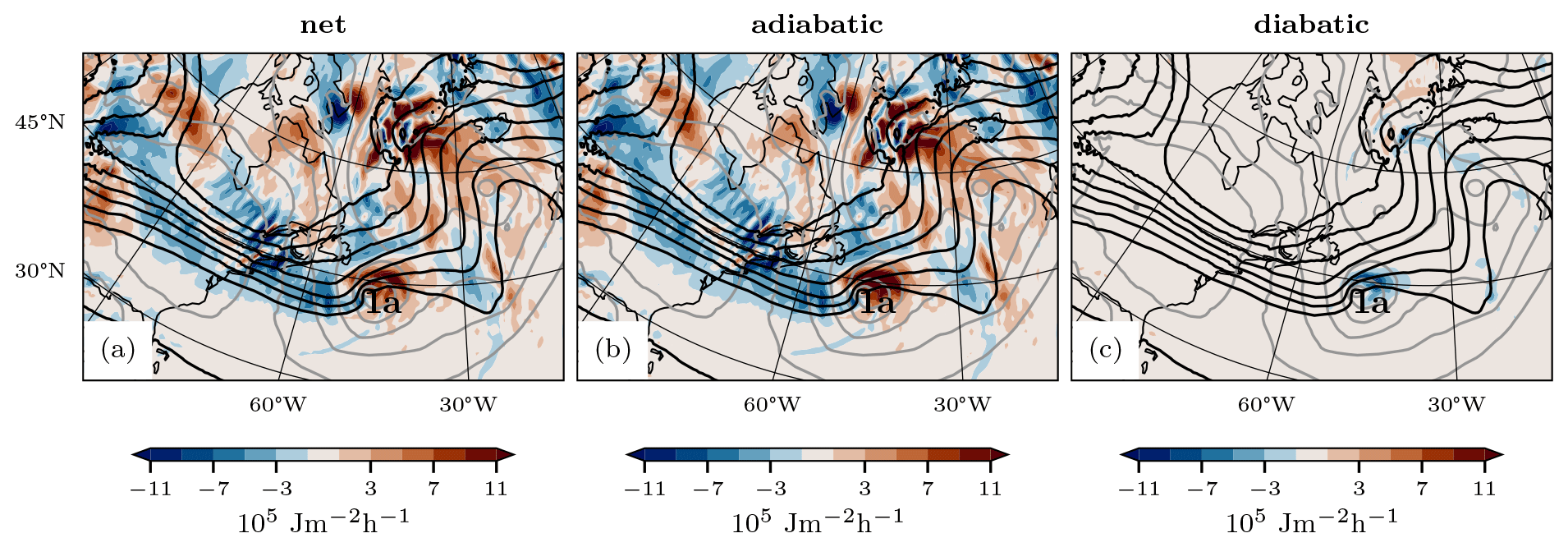
Figure 3 Vertically integrated instantaneous APE tendency on 19 February at 12:00 UTC (color shading). Shown are the (a) net change, (b) adiabatic contribution, and (c) diabatic contribution. Also shown are the vertically integrated APE distribution (black contours; same intervals as Fig. 1) and the mean sea-level pressure (grey contours; every 10 hPa). The location of cyclone 1a is indicated.

The largest net APE tendencies are concentrated at the edge of the polar reservoir and exhibit a complex pattern of negative and positive values. Therefore, it is challenging to identify the processes that give rise to instantaneous APE tendencies. In particular, the questions of where APE is supplied from remains open. We answer these questions using Lagrangian trajectories in the next sections.

3.2.2 Lagrangian APE tendency

To investigate the source regions of APE, we start 48 h forward trajectories at every grid point between 1000 and 250 hPa (every 10 hPa). Next we integrate the APE tendency forward along those trajectories, project this APE change onto the starting position of the respective trajectory, and integrate the resulting field vertically. This yields the Lagrangian APE change in a given column of air within the next 48 h, allowing us to identify the origin of the APE consumed at the edge of the polar APE reservoir. Figure 4 shows this vertically integrated Lagrangian 48 h change in APE from 19 February at 12:00 UTC to 21 February at 12:00 UTC. The character of the results does not change fundamentally if shorter integration times down to 24 h are chosen. Comparing the APE change (in color) with the APE distribution (black contours), in the case of a negative tendency, informs about the fraction of APE located at any given point which will be consumed in the following 48 h. Conversely, a positive tendency informs about the origin of air parcels which will experience an increase in APE. Note that this Lagrangian APE tendency does not indicate the change in the APE distribution at a given grid point, but the APE changes along the trajectories of air parcels, constituting a given column of air.

Figure 4 Vertically integrated 48 h forward APE change on 19 February at 12:00 UTC (color shading). Shown are the (a) net change, (b) adiabatic contribution, and (c) diabatic contribution. Also shown are the vertically integrated APE distribution (black contours; same intervals as Fig. 1) and the mean sea-level pressure (grey contours; every 10 hPa). The location of cyclone 1a is indicated. The regions indicated by the two black boxes in panel (b) show the start locations for trajectories evaluated in Fig. 5.

Generally, we observe that air parcels with high APE experience a loss of APE and air parcels with low APE experience a gain of APE. The net depletion of APE (Fig. 4a) is largest over eastern Canada. These air parcels are located within the APE reservoir adjacent to the Gulf Stream region, suggesting that this APE reservoir is most relevant to the supply of APE. Positive net APE changes are found at the boundary of the APE reservoir, in particular in the vicinity of cyclone 1a and a low-pressure system downstream.

The separation of the net tendency into adiabatic (vertical motion) and diabatic (diabatic heating and cooling) contributions reveals that the net tendency is dominated by the adiabatic tendency (Fig. 4b). Hence, vertical motion is responsible for the majority of the net APE tendency. The diabatic tendency (Fig. 4c) is weaker than the adiabatic tendency and exhibits a more complex pattern. First, we recognize a widespread pattern of a positive diabatic APE tendency toward the north and negative diabatic APE tendency toward the south. This pattern is due to radiative cooling of the free troposphere, which is reflected in an APE increase for air parcels colder than the reference state and an APE decrease for air parcels warmer than the reference state. This planetary-scale forcing of APE is interrupted by synoptic-scale regions of negative diabatic APE tendency within the APE reservoir and slightly downstream of cyclone 1a, which will be addressed in the next section.

This analysis demonstrates that the Lagrangian APE tendency in the vicinity of a cyclone shows a complex pattern of APE consumption and generation. In particular the intensification of the cyclone in this case study is accompanied by not only a loss of APE but also a gain of APE.

3.2.3 The motion of air parcels giving rise to APE tendencies

In order to understand the physical processes governing APE modification it is instructive to study the motion of the air parcels contributing to the APE budget. For this purpose, we select two regions of particularly high APE tendencies in the vicinity of cyclone 1a (Fig. 4b). The first region encompasses the APE reservoir over eastern Canada, for which we will consider air parcels which lose APE. The second region includes the warm sector of cyclone 1a, where we consider air parcels which gain APE. For both regions, we select the air parcels with the largest 48 h APE changes and which together account for 80 % of the vertically integrated APE loss and gain, respectively.

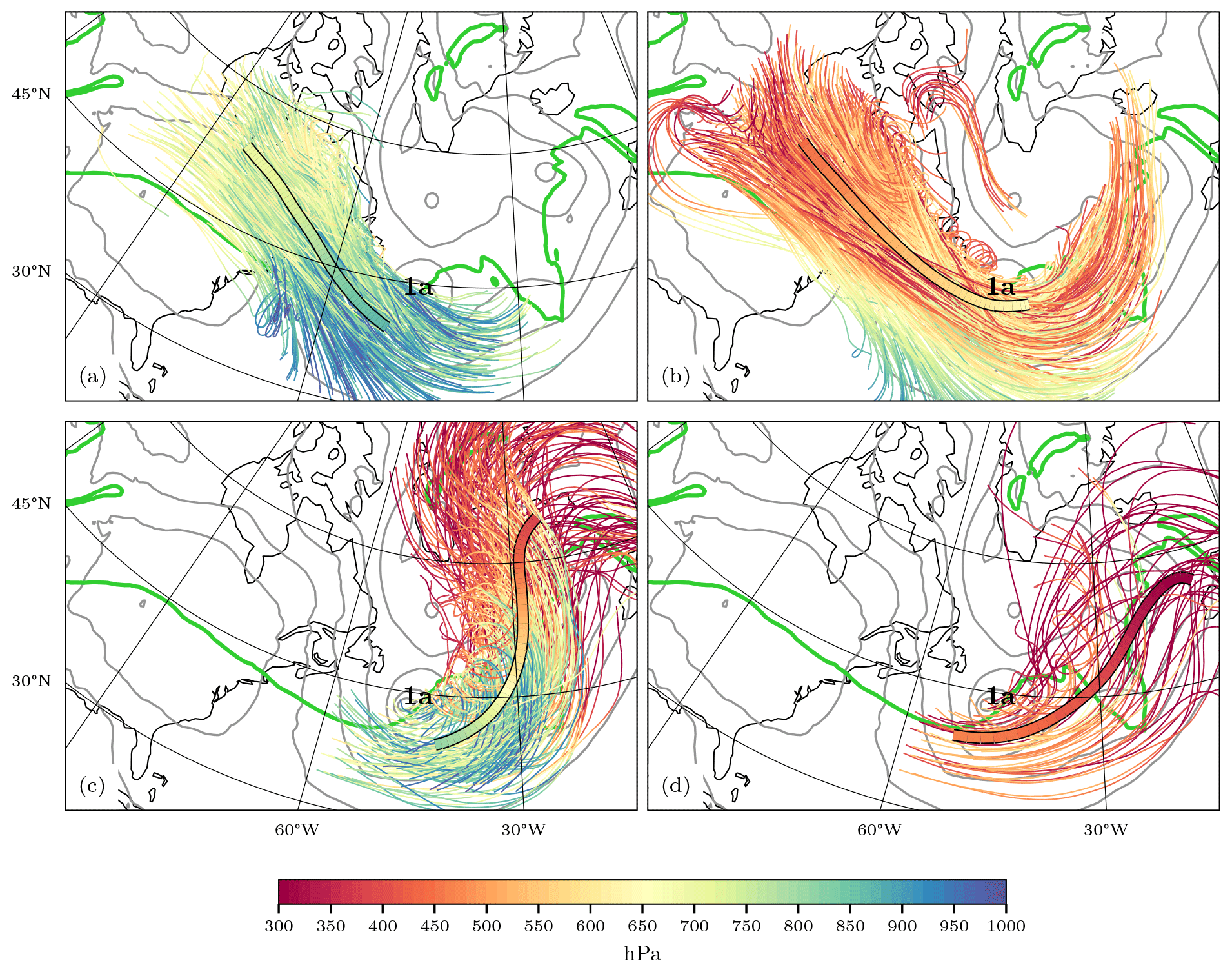
Figure 5 The 48 h forward trajectories (colored by pressure; every 10th trajectory) initialized (a, b) within the APE reservoir and (c, d) within the warm sector of cyclone 1a. Trajectories are split between starting locations in the (b, d) upper troposphere (p < 600 hPa) and (a, c) lower troposphere (p > 600 hPa). For each set of trajectories, a mean trajectory is shown. Also shown are the mean sea-level pressure (grey contours; every 10 hPa) and the 2 PVU contour on the 315 K isentrope (green). The location of cyclone 1a is indicated.

Trajectories started in the APE reservoir in the lower troposphere (p > 600 hPa; Fig. 5a) lose APE by descending in the North Atlantic behind the cold front of cyclone 1a. Trajectories started in the APE reservoir in the upper troposphere (p < 600 hPa; Fig. 5b) show different behavior. Some trajectories descend strongly and arrive in the lower troposphere behind the cold front of cyclone 1a. But other trajectories descend weakly and are advected around the upper-level trough. Still all trajectories contribute significantly to the decrease in vertically integrated APE.

Trajectories started in the second region within the lower troposphere (p > 600 hPa; Fig. 5c) ascend strongly from within the warm sector of cyclone 1a until they reach the upper troposphere and outflow into the upper-level ridge downstream of cyclone 1a. Since the ascending air parcels gain APE, they must be colder than their reference state, which suggests that the ascent occurs in anomalously cold air with respect to the reference state. The rapid ascent of these trajectories is reminiscent of a warm conveyor belt (WCB), which is associated with strong latent heat release. Indeed, the region of negative diabatic APE tendency observed slightly downstream of cyclone 1a coincides with the ascending air parcels. This also implies that the thermal efficiency of the air parcels must be negative, which means that the air parcels are colder than their reference state. Therefore, latent heat release in the ascending airstream leads to a destruction of APE. Lastly, trajectories started in the second region within the upper troposphere (p < 600 hPa; Fig. 5d) tend to start upstream of cyclone 1a and ascend into the upper troposphere. Since they already start at high altitudes, they cannot ascend as much as trajectories from the lower troposphere, but they still account for significant APE production.

The trajectories highlight the role of the upper-level dynamics for the APE budget. While air parcels in the upper troposphere require little vertical motion to yield a significant change in APE, air parcels from within the lower troposphere require large vertical displacements to contribute substantially to the local APE budget. Figures S3–S5 in the Supplement show the detailed evolution of the APE tendency along selected trajectories from Fig. 5. In particular, the efficiency is key in determining the resulting APE tendency from a given vertical motion. The adiabatic efficiency, for instance, is larger in the upper troposphere (because there is a lot of APE). Therefore, small vertical displacements can lead to large adiabatic APE tendencies.

The trajectories in Fig. 5a and b also explain why we observe a second maximum of diabatic APE loss (Fig. 4c) over eastern Canada. Many trajectories, in particular from the lower troposphere, descend to 800 hPa or even lower, where they likely enter the boundary layer. Even though not all of them are directly exposed to heat fluxes at the surface, they are heated in the boundary layer above the Gulf Stream SST front due to mixing processes (also see Fig. S5 in the Supplement). This heating dissipates more APE than is gained through radiative cooling, which is why the 48 h integrated diabatic APE tendency is negative in some regions of eastern Canada (Fig. 4c).

3.2.4 Dry-dynamic forcing of the APE tendency

Since the APE density is largest in the upper troposphere, we next study the quasi-geostrophic forcing due to the large-scale upper-tropospheric circulation. Figure 6 shows the positions of ascending and descending trajectories between 400 and 600 hPa and the upper-level QGω forcing at 500 hPa at two time steps. On 20 February at 00:00 UTC (Fig. 6a) the pattern of QGω shows a dipole structure of ascent on the eastern flank and descent on the western flank of the trough. The upward QGω forcing is concentrated above the center of cyclone 1a, whereas the downward QGω forcing extends westward along the poleward side of the jet stream. As cyclone 1a moves further poleward on 20 February at 12:00 UTC (Fig. 6b) the dipole structure in QGω collocated with cyclone 1a is separated from the band of downward QGω forcing on the eastern flank of the trough. Thus, large parts of the downward ageostrophic circulation due to the trough do not remain collocated with the surface cyclone during its life cycle. In contrast, the QGω forcing due to lower levels moves with the surface cyclone but is much weaker than the forcing from upper levels (Fig. S2 in the Supplement).

Figure 6 Upper-level quasi-geostrophic ω on 500 hPa (color shading) for two time steps. Descending (×) and ascending (⋅) trajectory positions for every 10th trajectory are marked in black as they reach the layer between 400 and 600 hPa. Also shown are the 2 PVU contour on the 315 K isentrope (green) and wind speed at 300 hPa (black contours; 60, 80, and 100 m s⁻¹). The location of cyclone 1a is indicated.

The positions of the descending trajectories show that they are affected by downward QGω forcing as they descend. On 20 February at 00:00 UTC (Fig. 6a) the majority of trajectories descend along the downstream flank of the upper-tropospheric ridge, predominantly on the poleward side of the jet axis, while few trajectories descend further south in the vicinity of cyclone 1a. In the meantime the ascending trajectories are collocated with the upward QGω forcing around cyclone 1a. On 20 February at 12:00 UTC (Fig. 6b) the majority of descending trajectories remain within the influence of the downward QGω forcing beneath the upper-level jet, while none of the selected trajectories descend directly within cyclone 1a. In contrast, the ascending trajectories continue their ascent around cyclone 1a due to the upward QGω forcing.

The close association of the movement of air parcels and the QGω forcing from upper levels indicates that the redistribution of air parcels in the vicinity of cyclone 1a, which leads to the observed APE tendencies, is a result of the circulation at upper levels. In particular, the loss of APE along the western flank of the trough is closely connected to the ageostrophic circulation. Therefore, the depletion of the APE reservoir shown in Fig. 4 takes place not directly within cyclone 1a but rather at the western flank of the trough.

3.3 The role of air–sea interaction

Many air parcels which start in the APE reservoir and lose APE as they descend eventually arrive in the lower troposphere, where they experience diabatic warming due to the interaction with the warm waters of the Gulf Stream SST front (Fig. 5a, b). The air parcels lose APE through their descent, since they are colder than their reference state. Therefore, diabatic warming of those air parcels should result in the destruction of APE, which decreases the amount of APE available for conversion to KE. In order to test this hypothesis, we start 48 h backward trajectories within the boundary layer of the strong marine CAO on 20 February at 12:00 UTC, where we expect the largest surface fluxes of heat. Figure 7 shows that indeed the selected trajectories descend into the CAO region and are of continental origin.

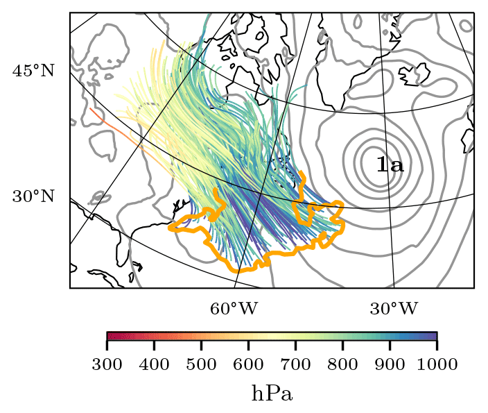
Figure 7 The 48 h backward trajectories (colored by pressure; every 10th trajectory) initialized in the CAO area south of 50° N within the boundary layer on 20 February at 12:00 UTC. The 8 K contour of the CAO index south of 50° N is shown in orange. Also shown is the mean sea-level pressure (grey contours; every 10 hPa).

The air parcels arriving within the CAO typically start their descent between 900 and 600 hPa within the poleward reservoir of high-APE air. Thus, the air parcels feature a significant APE density 48 h before they arrive within the CAO, which is almost entirely depleted upon their arrival in the CAO (Fig. 8a). On average, the air parcels descend by more than 100 hPa (Fig. 8b), which results in a negative adiabatic APE tendency (Fig. 8c). In contrast to the adiabatic tendency, the average diabatic tendency of APE becomes negative only 12 h before arrival in the CAO, when the air parcels start to be exposed to diabatic heating via surface sensible heat fluxes and latent heating. Moreover, the magnitude of the diabatic tendency is a factor of 4 smaller than the adiabatic tendency (Fig. 8d). Even though the warming of air parcels within the CAO might be strong, the air parcels are already close to their reference state because of the adiabatic descent prior to their arrival in the CAO. Therefore, the air parcels have a low APE density and a low thermal efficiency. Since the diabatic tendency is given by the product of the diabatic heating rate and the thermal efficiency, even large heating rates do not result in a large diabatic APE tendency. Thus, locally, the high APE of the upper tropospheric polar cold air is primarily converted to KE rather than depleted by diabatic air mass transformations.

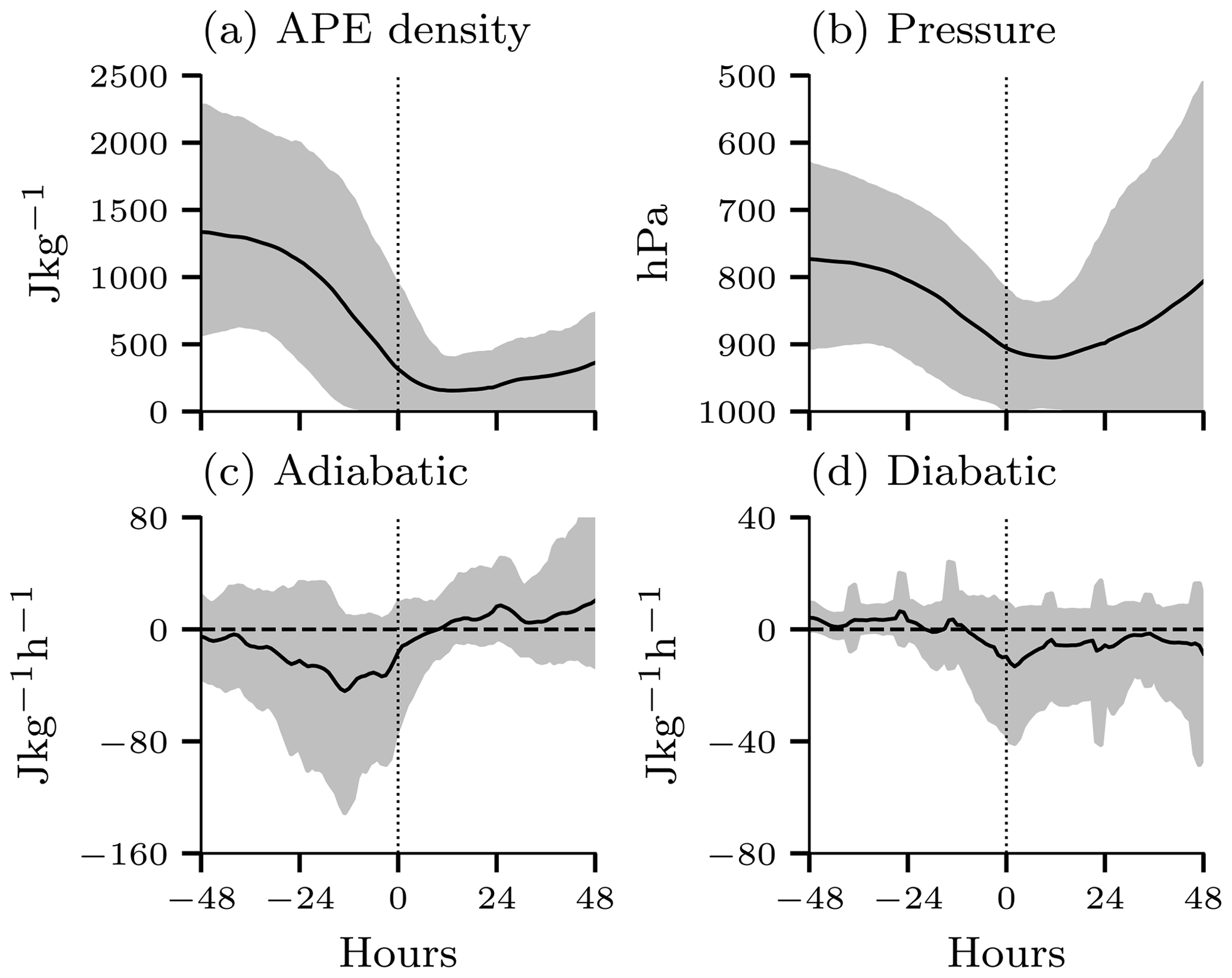
Figure 8 Evolution of the (a) APE density, (b) pressure, (c) adiabatic APE tendency, and (d) diabatic APE tendency of CAO trajectories that started on 20 February at 12:00 UTC centered on their arrival in the CAO region (time at 0). Note the different scales of the tendency in panels (c) and (d). The solid black line indicates the mean, and the grey shading denotes the range between the 5th and 95th percentile of the trajectories.

3.4 Key characteristics of APE on synoptic scales

Before turning our attention to the climatological analyses, we aim here to briefly summarize our findings from the case study. In light of the three questions posed in the Introduction, we can draw the following conclusions regarding local APE during a period of rapid North Atlantic cyclogenesis:

• Cyclones within the case study period develop at the edge of the polar APE reservoir. The intensification of the cyclones is associated with an extension of this APE reservoir into the North Atlantic in the wake of the cyclones. This APE is located in the middle to upper troposphere, below the upper-level trough to the west of the surface cyclone.

• The vertical motion induced by the interaction of the intensifying surface cyclone and upper-level trough lead to both APE consumption and production. APE is primarily consumed by the descent along the western flank of the trough, while APE is produced by the ascent ahead of the trough. This pattern of ascent and descent is consistent with QGω forcing by upper levels. Therefore, the majority of APE conversion takes place through the circulation in the middle to upper levels and not within the surface cyclone itself.

• The diabatic dissipation of APE induced by surface fluxes is predominantly confined to the lower troposphere. By the time air parcels have reached the lower troposphere, the bulk of APE has already been consumed adiabatically. Therefore, the impact of surface fluxes on the local APE budget is small compared to the previous conversion into KE via subsidence due to low thermal efficiency.

In the next section, we will explore the validity of those findings for deep North Atlantic cyclones in general.

4 Climatology

For the climatological analysis, our focus is on strongly intensifying Gulf Stream cyclones. First, we identify all cyclones in the study period (DJF) with a lifetime of at least 24 h which reach their maximum intensification rate within 24 h in the defined Gulf Stream region, bounded by 30–55° N and 80–30° W. Subsequently, from this set of cyclones, we select the 20 % deepest ones, where the depth is defined as the difference in mean sea-level pressure between the outermost closed contour and the pressure minimum (Fig. 9b). This results in a total of 285 cyclone tracks, as illustrated in Fig. 9a.

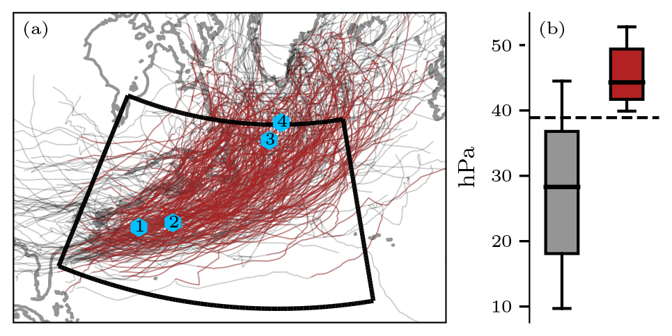
Figure 9 (a) Selected cyclone tracks within the Gulf Stream region, indicated by the black box. The section of the tracks between 12 h before maximum intensification and 12 h after maximum depth is highlighted in red. Blue hexagons mark the mean locations where the cyclones experience maximum deepening over 24 h (2) and maximum depth (3), as well as 12 h before (1) and after (4). (b) Distribution of maximum depth for cyclones attaining maximum intensification within the Gulf Stream region for all cyclones (grey) and the 20 % deepest cyclones (red). Whiskers show the range of the 10th–90th percentiles. The dashed black line indicates the 80th percentile of the climatological maximum depth of Gulf Stream cyclones, which was used as a selection criterion.

Our selection process minimizes variability among the chosen cyclones. First, the geographical criterion ensures a focus on Shapiro–Keyser cyclones (Shapiro and Keyser, 1990) that predominantly propagate poleward along the Gulf Stream sea-surface temperature (SST) front (Fig. 9a). Second, the intensity criterion ensures that only cyclones of substantial strength are selected, facilitating more direct comparisons and minimizing variability in our composite study.

4.1 Cyclone-centered composites

4.1.1 Cyclone life cycle

Figure 10 depicts cyclone-centered composites of Gulf Stream cyclones for various stages of their life cycle, anchored on the time of maximum intensification (Δp_max) and maximum depth (d_max). We define the time 12 h before Δp_max is reached as the onset stage and the time 12 h after d_max is reached as the decay stage. Analysis of average fields of isentropic PV at 315 K and horizontal wind speed at 300 hPa reveals distinctive characteristics at these different stages of the cyclone life cycle.

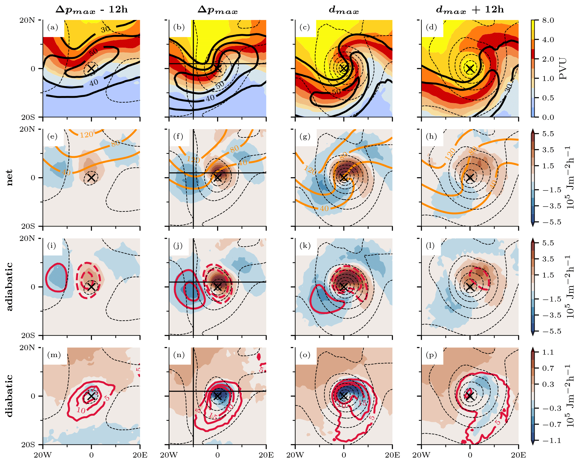
Figure 10 Cyclone-relative composites 12 h before the time of maximum intensification (Δp_max − 12 h), at the time of maximum intensification (Δp_max), at the time of maximum depth (d_max), and 12 h after the time of maximum depth (d_max + 12 h). Dashed black contours indicate mean sea-level pressure (every 8 hPa). (a–d) Isentropic PV at 315 K (shading) and wind speed at 300 hPa (black contours; every 10 m s⁻¹). (e–h) Net APE tendency (shading) and the distribution of vertically integrated APE density (orange contours; 40, 80, 120 × 10⁵ J m⁻²). (i–l) Adiabatic APE tendency (shading) and upper-level QGω at 500 hPa (red contours; −0.1, −0.05, 0.05, 0.1 Pa s⁻¹). (m–p) Diabatic APE tendency (shading) and 1 h accumulated precipitation (red contours; every 5 mm). Note the different color scales for the APE tendencies. Black lines indicate the location of cross sections in Fig. 12.

At the onset, the cyclone center is located ahead of an upper-level trough (Fig. 10a). By the time the cyclone reaches Δp_max, the trough has intensified and the cyclone has crossed the jet axis (Fig. 10b). Upon reaching d_max, the cyclone is located at the left exit of the jet, accompanied by upper-level cyclonic Rossby wave breaking and yielding a ridge downstream of the cyclone (Fig. 10c); 12 h later, the cyclone enters the decay phase, characterized by a vertically stacked cyclonic circulation with no vertical tilt (Fig. 10d).

4.1.2 Horizontal APE evolution

The cyclone typically is found at the southern boundary of the APE reservoir at the onset stage (Fig. 10e). The vertically integrated net APE tendency shows a weak dipole pattern with APE production near the cyclone center and consumption upstream with amplitudes of 2.5 × 10⁵ J m⁻² h⁻¹. As the cyclone intensifies, the APE reservoir extends farther south relative to the cyclone center, accompanied by an intensification of the APE tendency dipole (Fig. 10f). At d_max the positive APE tendency reaches an amplitude of 9 × 10⁵ J m⁻² h⁻¹ compared to only to only −4.5 × 10⁵ J m⁻² h⁻¹ for the negative tendency (Fig. 10g). Furthermore, the negative APE tendency extends downstream of the cyclone. A comparison with the PV field at d_max (Fig. 10c) reveals that the cyclone is part of a dispersive baroclinic wave, manifesting in the formation of another trough downstream of the cyclone. Consequently, the negative APE tendency downstream is indirectly linked to the cyclone via downstream development. During the decay of the cyclone, the APE tendencies weaken significantly (Fig. 10h).

Throughout the cyclone's life cycle, the evolution of vertically integrated APE closely follows the development of the upper-level trough, reinforcing findings from the case study that underscore the close connection between the upper-level large-scale circulation and the APE distribution. Additionally, our analysis indicates a consistent pattern of APE consumption at the western flank of the trough and APE production at the eastern flank of the trough.

Next, we decompose the net APE tendency into its adiabatic and diabatic components and investigate the atmospheric conditions driving these tendencies. For all stages of the cyclone life cycle, the adiabatic APE tendency shows a pattern and amplitude closely resembling that of the net APE tendency. This reaffirms findings from the case study: the dominant role of the adiabatic contribution in the APE budget, suggesting that the net change in APE predominantly stems from vertical motion. This is also in line with upper-level QGω forcing. In fact, during the onset phase, the upper-level QGω forcing at 500 hPa indicates forcing for ascent ahead of the trough and a forcing for descent behind it, aligning closely with the adiabatic APE tendency (Fig. 10i). As the cyclone reaches Δp_max, there is an increase in the magnitude of upper-level QGω forcing, reflected in substantial adiabatic APE tendencies (Fig. 10j). At d_max the weaker negative adiabatic APE tendency compared to the positive APE tendency is consistent with the upper-level QGω forcing (Fig. 10k). A total of 12 h later, the decay of the surface cyclone coincides with a decrease in the upper-level QGω forcing (Fig. 10l). Notably, the upward forcing is displaced from the cyclone center, indicating a weakened coupling between upper and lower levels, which also translates to smaller adiabatic APE tendencies. The close association between the upper-level QGω forcing and the adiabatic APE tendency corroborates the findings of the case study, suggesting that APE changes are primarily driven by upper-level dynamics.

Finally, the diabatic APE tendency exhibits a north–south dipole background associated with radiative cooling of the free troposphere, wherein APE is generated toward the poles and dissipated toward the Equator (Fig. 10m). The diabatic generation of APE reaches an amplitude of 0.6 × 10⁵ J m⁻² h⁻¹, which is significantly weaker than the observed adiabatic APE tendencies. The diabatic APE generation due to radiative cooling increases between the times Δp_max and d_max when the poleward displacement of the mean composite location is largest (Fig. 9). This means that the environment of the cyclone becomes colder with more negative thermal efficiency. Thus, the radiative cooling leads to larger diabatic APE generation. Superposed on this background pattern is a pronounced negative diabatic APE tendency in the cyclone's warm sector (Fig. 10n–p). Notably, this negative diabatic APE tendency coincides with intense precipitation, wherein latent heat release warms the air colder than its reference state, consequently leading to APE destruction of up to −3 × 10⁵ J m⁻² h⁻¹ at the time of Δp_max. Therefore, the negative diabatic APE tendency due to latent heat release is much larger than the background pattern due to radiative cooling and significantly counteracts the positive adiabatic APE tendency due to ascent. This finding is also consistent with observations from the case study.

4.1.3 Evolution of the net APE tendency

As the cyclone intensifies, the relative magnitude of the positive and negative local contributions to the net APE tendency changes (Fig. 10e–h). To quantify this evolution, we compute the volume integral of the net tendency for each cyclone within a 2000 km radius around the cyclone center (which corresponds to a radius of approximately 20° in Fig. 10) and compare it with the intensification of the cyclone. Figure 11a shows the distribution of the mean sea-level pressure minimum (p_min) of the selected cyclones during the four stages of their life cycle. By design, the strongest deepening takes place around the time of Δp_max until the maximum depth d_max is reached. Between the time of d_max and d_max + 12 h the minimum pressure increases, which indicates the decay of the surface cyclone and a weakening of the circulation.

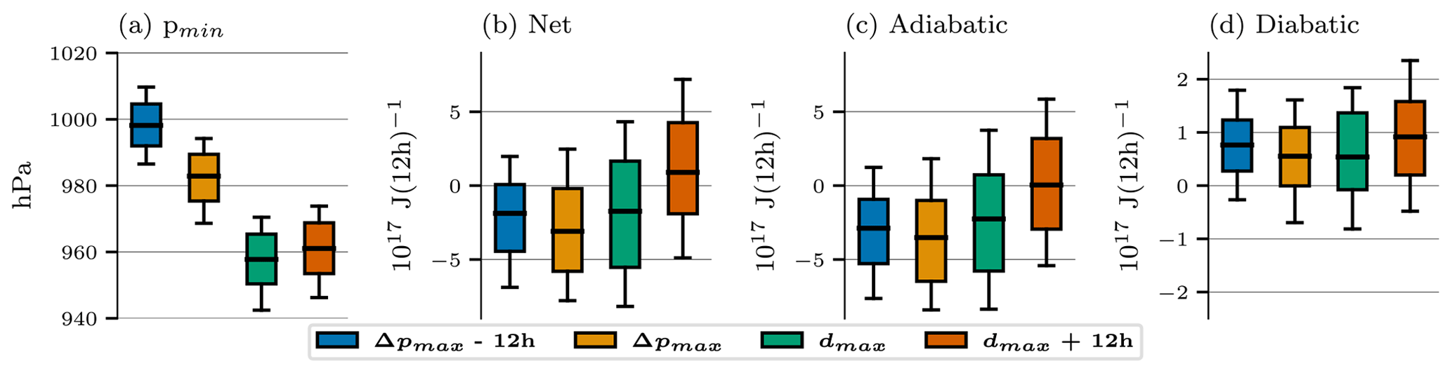
Figure 11 (a) Distribution of minimum mean sea-level pressure of the 285 selected cyclones, averaged ±6 h around the four life cycle stages. The (b) net, (c) adiabatic, and (d) diabatic APE tendency is integrated in a 2000 km radius around the cyclone center within a ±6 h window around the four life cycle stages. Whiskers show the range of the 10th–90th percentiles.

The integrated net APE tendency, averaged over a 12 h window centered on the selected life cycle stages, is depicted in Fig. 11b. Between the onset stage and the time of Δp_max, the net tendency becomes more negative, indicating that the conversion of APE to KE intensifies. At the time of Δp_max, the net tendency reaches a minimum, which is consistent with the observation that this is the stage in which the strongest intensification of the cyclone occurs. Subsequently, the net tendency becomes more positive as the intensification weakens prior to the time of d_max, which marks the beginning of the decay phase of the cyclone. This is reflected in a sharp increase in the net tendency, which becomes positive 12 h after d_max. At this stage, the net conversion is from KE back to APE. Hence, the intensification of the surface cyclone is reflected in the life cycle of the net APE tendency in the vicinity of the cyclone.

Consistent with the horizontal evolution of the APE tendency, the integrated net APE tendency is largely adiabatic (Fig. 11c). This indicates that the net APE tendency is determined by the balance between the negative adiabatic APE tendency due to descent along the western flank of the trough and the positive tendency due to ascent along the eastern flank of the trough. As the cyclone intensifies, more APE is converted to KE by descent than KE is converted back to APE by ascent, resulting in a net increase in KE. However, once the cyclone has reached its maximum intensity (d_max) and begins to decay, this balance shifts in favor of the positive tendency due to ascent, leading to a net decrease in KE.

The life cycle is somewhat less apparent in the adiabatic tendency compared to the net tendency. This discrepancy can be attributed to the diabatic contribution (Fig. 11d), which reaches a minimum at the time of Δp_max yet stays net positive throughout the cyclone's life cycle. This accentuates the evolution observed for the adiabatic tendency. The diabatic tendency is positive due to the creation of APE by radiative cooling of the free troposphere on the cold side of the baroclinic zone, which is largely independent of cyclogenesis. Consequently, the reduction in the diabatic tendency as the cyclone intensifies is attributable to the latent heat release in the ascending airstream of the cyclone, which dissipates APE as it warms air that is colder than its reference state.

Despite the clear life cycle being recovered from the integrated net APE tendency, the spread is wide. This is due to the fact that APE conversion is closely linked to the large-scale circulation, as discussed in the previous section. Therefore, the extraction of KE does not have to occur in the immediate vicinity of the surface cyclone. For instance, it can occur at the entrance of the jet stream, which can be located at a considerable distance from the cyclone if the cyclone intensifies at the jet exit (cf. Fig. 10b). In contrast, APE production through the ascending airstream occurs in close proximity to the center of the cyclone. Therefore, the analysis is also sensitive to the choice of the integration radius. A smaller radius changes the observed life cycle because regions of APE consumption are excluded, whereas a larger radius does not (Figs. S8–S10 in the Supplement).

4.1.4 Vertical APE structure

The vertical structure of the cyclone-relative composites is illustrated in Fig. 12 through both meridional and zonal cross sections at the time of maximum intensification. The horizontal location of the cross sections is indicated in Fig. 10. The meridional cross section shows the surface cyclone slightly poleward of the baroclinic zone and the upper-level jet stream because the cross section cuts through the cold sector of the cyclone (Fig. 12a). Also the height of the tropopause, marked by the 2 PVU line, is constant poleward of the baroclinic zone but increases steeply in the baroclinic zone. The APE density is concentrated on the poleward side of the cyclone below the tropopause, where the air is much colder than its reference state (Fig. 12b). The APE density decreases toward the surface, reaching its minimum in the lower troposphere. The negative adiabatic APE tendency spans from 850 to 250 hPa, peaking around 500 hPa. Conversely, the diabatic APE tendency is positive throughout much of the free troposphere north of the baroclinic zone, contributing to the maintenance of the poleward APE reservoir (Fig. 12c).

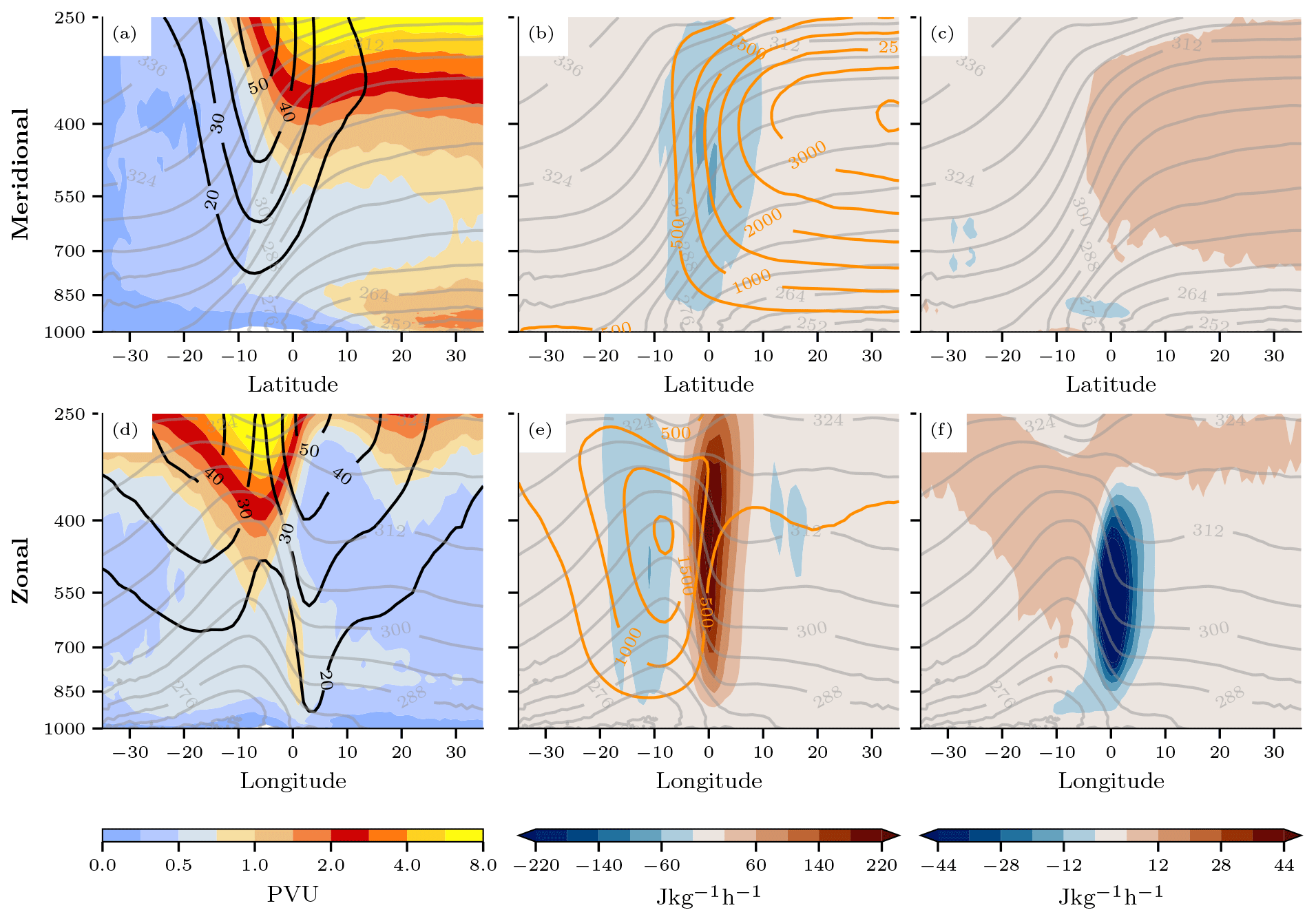
Figure 12 Cross sections of cyclone-centered composites at the time of maximum intensification. Panels (a)–(c) are meridional cross sections at 10° W (ca. 1000 km west), and panels (d)–(f) are zonal cross sections at 2° N (ca. 200 km north) relative to the cyclone center. (a, d) PV (shading) and horizontal wind speed (black; every 10 m s⁻¹). (b, e) Adiabatic APE tendency (shading) and APE density (orange contours; every 500 J kg⁻¹). (c, f) Diabatic APE tendency. Potential temperature is indicated by grey contours (every 6 K). The locations of the cross sections are indicated in Fig. 10.

Examining the zonal cross section of the PV field reveals the presence of the upper-level trough upstream of the cyclone center, alongside jet cores flanking it (Fig. 12d). Below the trough, isolines of potential temperature are bent upward, indicative of a cold anomaly beneath the trough, where APE density is maximal (Fig. 12e). Both the positive and negative adiabatic APE tendencies extend through most of the column, peaking around 500 hPa. Given the negative adiabatic APE tendency within regions of high APE density and positive APE tendency downstream in the area of low APE density, the dipole of APE tendency leads to an eastward propagation of the APE density maximum. Furthermore, the diabatic APE tendency is most pronounced where the largest positive adiabatic APE tendency is observed (Fig. 12f) such that the diabatic APE tendency partially offsets the adiabatic APE tendency. In fact, the ascent leading to the positive adiabatic APE tendency also leads to considerable latent heat release, which translates to the negative diabatic APE tendency.

4.2 The role of surface fluxes for the diabatic APE tendency

Apart from latent heat release, surface sensible heat fluxes present a major source of heat for the atmosphere in the Gulf Stream region. To clarify the climatological role of surface fluxes along the Gulf Stream front in the APE budget, we focus on marine CAOs associated with Gulf Stream cyclones, which are typically accompanied by substantial latent and sensible heat fluxes. We identify CAOs as areas where the CAO index exceeds 8 K and that lie within 30–50° N and 130–30° W at the time of maximum intensification of the cyclones. From within these identified regions, we initiate 2 d forward and 5 d backward trajectories at each grid point between 1000 hPa and the boundary layer height in 25 hPa intervals. Of the sample of 285 cyclones, all but 26 were accompanied by a CAO. The mean trajectory evolution, centered on the first time step when trajectories reach a CAO index surpassing 8 K, is depicted in Fig. 13.

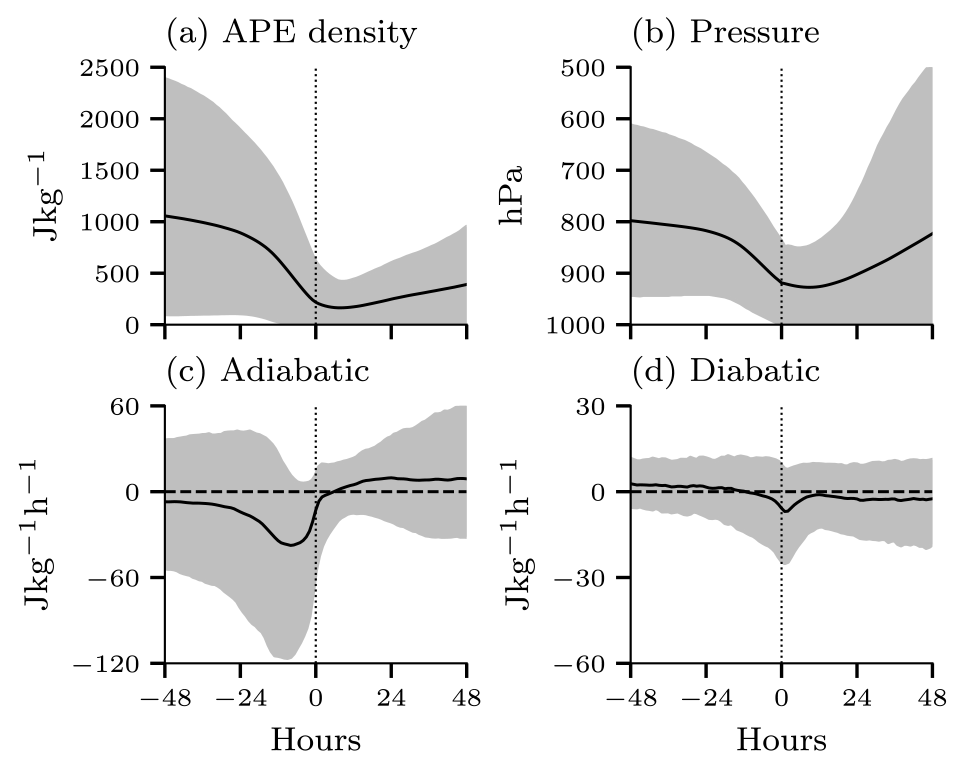
Figure 13 Evolution of the (a) APE density, (b) pressure, (c) adiabatic APE tendency, and (d) diabatic APE tendency of CAO trajectories centered on their arrival in the CAO region (time at 0). The solid black line indicates the mean, and the grey shading denotes the range between the 5th and 95th percentiles of the trajectories. Note the different scales of the tendency in panels (c) and (d). For details about the trajectory calculation, see the text.

The mean APE density of the air parcels exhibits a continuous decrease over the 48 h period preceding their arrival in the CAO, reaching a minimum approximately 6 h later (Fig. 13a). Concurrently, the mean pressure along trajectories indicates that this APE decrease coincides with a descent of approximately 100 hPa (Fig. 13b), reflected in the negative adiabatic APE tendency prior to arrival in the CAO (Fig. 13c). In contrast, the diabatic APE tendency remains slightly positive and only transitions to negative values 12 h before the air parcels arrive in the CAO (Fig. 13d). By the time the negative diabatic APE tendency peaks, the majority of the APE has already been depleted by the descent of air parcels into the CAO. Thus, the climatological analysis confirms the observation from the case study that surface fluxes act as a sink of APE, although their magnitude is small compared to the adiabatic conversion of APE to KE.

5 Conclusions

5.1 Synthesis

In this study, we have conducted an analysis of the spatial distribution and temporal tendencies of local APE density within a dataset comprising 285 intense North Atlantic cyclones that undergo intensification in the Gulf Stream region. Our investigation has focused on elucidating the interplay between local APE and large-scale atmospheric circulation while also evaluating the impact of the intense air–sea interaction in the Gulf Stream region on the local APE budget. The principal findings of our analysis can be summarized as follows:

• Intense Gulf Stream cyclones typically originate at the edge of the polar APE reservoir. The baroclinic interaction of those cyclones with upper-level troughs induces a cold anomaly in the middle to upper troposphere beneath the trough. This cold anomaly serves as a reservoir of high-APE air, which is transported from polar latitudes to midlatitudes and provides the energy for baroclinic conversion.

• While APE is predominantly consumed adiabatically through descent along the western flank of the upper-level trough, it is concurrently generated by ascent ahead of the trough. This dipole of adiabatic APE tendencies aligns closely with the ageostrophic vertical circulation induced by the trough, thereby highlighting the intimate connection between the local APE budget and the upper-tropospheric large-scale atmospheric circulation. Furthermore, the release of latent heat in the ascending airstream in the cyclone's warm sector leads to a negative diabatic tendency, resulting in the destruction of APE. Consequently, latent heat release acts as a sink for APE.

• Our Lagrangian trajectory analysis of the influence of air–sea interaction on the local APE budget reveals that the bulk of APE is converted to KE during descent prior to air parcels experiencing surface fluxes within CAOs. Therefore, comparatively little APE is dissipated by surface sensible heat fluxes in the lower troposphere.

In conclusion, our study underscores the significant influence of synoptic-scale circulation patterns on the distribution of local APE. We observe complex patterns of APE tendency, largely following the trough and ridge patterns aloft. These ensue from the ageostrophic circulation induced by large-scale flow features such as upper-level troughs and ridges and their baroclinic interactions with the lower troposphere.

5.2 Discussion

A novelty of our work is the coupling of global energetics with the large-scale circulation and PV thinking (Hoskins et al., 1985). We show that, locally, midlatitude APE is found in the cold anomaly below an upper-level trough. Therefore, isentropic lifting below upper-level troughs, termed the “vacuum cleaner” effect in Hoskins et al. (1985), links the distribution of APE and PV. The distribution of PV is also linked to the adiabatic APE tendency via the ω equation (Hoskins et al., 2003). As a midlatitude PV anomaly propagates eastward in a baroclinic zone, it leads to descent at the western flank and ascent at the eastern flank of the anomaly, corresponding to a negative APE tendency west of the anomaly and a positive APE tendency east of the anomaly. Therefore, APE is converted to KE upstream of the anomaly, where the flow is accelerated. In turn, the deceleration of the flow downstream of the anomaly means that KE is converted back to APE, effectively propagating the maximum APE below the upper-level trough. From that perspective, the upper-level flow controls the distribution of APE. In addition to the curvature associated with an upper-level PV anomaly, other synoptic environments can contribute to ageostrophic vertical circulations and influence APE tendencies. For instance, the thermally direct transverse circulation in the entrance region of a jet streak is expected to convert APE into KE, while the thermally indirect transverse circulation at the jet exit would convert KE back into APE. Furthermore, temperature advection across the jet can influence the location of the ageostrophic vertical circulation (Keyser and Shapiro, 1986), thereby affecting the associated APE tendencies.

Our study differs substantially from previous works on the atmospheric energy cycle in that we consider the total APE rather than a decomposition into mean and eddy APE. While a decomposition into mean and eddy contributions facilitates the interpretation of climatological APE conversions, these conversions cannot readily be attributed to individual weather systems on synoptic charts. Nevertheless, we recover some fundamental patterns in the climatology of APE tendencies shown in Novak and Tailleux (2018) within our cyclone-relative perspective. Novak and Tailleux (2018) identify a hot spot of adiabatic conversion of eddy APE to eddy KE at the upstream edge of the North Atlantic storm track, where the large-scale flow is generally accelerated and the entrance of the climatological jet stream is found (Koch et al., 2006). This is consistent with our finding that the adiabatic APE tendency in cyclones is negative along the western flank of the upper-level trough, where the large-scale flow is accelerated. Novak and Tailleux (2018) also find that the conversion from mean KE to mean APE is largest in the downstream part of the North Atlantic storm track, where the exit of the climatological jet stream is located (Koch et al., 2006). This is consistent with Bowley et al. (2019), who identified ascent on the poleward flank of the wave guide in the exit region of the North Pacific jet stream as a mechanism for zonal APE buildup. We show that the positive adiabatic tendency is greatest in the decay phase of cyclones ahead of the upper-level trough, where the large-scale flow is decelerated. Thus, our results show how individual cyclones can contribute to the climatological patterns of APE conversion.

A consequence of abandoning the eddy-mean decomposition is that the ascending airstream near the cyclone center converts KE back into APE, which is counterintuitive given that the rising airstream originates in a local warm anomaly. However, this result is consistent with the local APE framework because the global reference state is similar to a spatial average of potential temperature on pressure surfaces. Thus, the ascent occurs within negative adiabatic efficiency with respect to the global reference state. In contrast, the eddy-mean decomposition introduces a temporal average of the reference state, which allows for a physically more localized interpretation of the conversion of eddy APE to eddy KE because it accounts for high-frequency warm and cold anomalies introduced by the meridional circulation around a low-pressure system. However, it is difficult to attribute eddy and mean conversions to individual weather systems.

Novak and Tailleux (2018) have also shown that in the North Atlantic, the diabatic mean and eddy APE tendencies are largest along the storm track. However, the mean component destroys APE, while the eddy component generates APE, obscuring the net effect on the total APE. We show that the total diabatic APE tendency due to latent heat release in the warm sector of cyclones is negative because the latent heat release occurs in air which is colder than its reference state. Since the local APE density is derived from the dry hydrostatic primitive equations, the feedback of diabatic heating on the vertical velocity (Nie and Sobel, 2016; Li and O'Gorman, 2020) is not explicitly captured. Therefore, we hypothesize that the negative diabatic APE tendency due to latent heat release is smaller than the enhancement of the adiabatic APE tendency due to stronger updrafts, which would reconcile our result with the fact that latent heat release generally accelerates cyclone development (Schemm et al., 2013; Binder et al., 2016). This result also follows from moist APE frameworks, which include the potential of latent heat release in APE (Lorenz, 1979; Gertler and O'Gorman, 2019; Gertler et al., 2023). However, a moist atmosphere may have several local minima of potential energy, which makes the definition of a unique APE density difficult (Tailleux, 2013).

Even for the dry APE density, the choice of a reference state is not straightforward (Shepherd, 1993; Tailleux, 2018). Federer et al. (2024) computed a reference state for a baroclinic channel, where the baroclinic zone is approximately in the center of the channel. Therefore, the APE reservoirs on the poleward and equatorward sides of the baroclinic zone have similar APE densities and are equally important as APE source regions for the development of the baroclinic wave. In contrast, Earth's spherical geometry means that there is more mass on the warm side than on the cold side of the midlatitude baroclinic zone. Consequently, the Lorenz reference state constructed from Earth's atmosphere yields a high APE density on the cold side and a low APE density on the warm side of the baroclinic zone. This explains why we identify the equatorward descent of cold air as the main extraction mechanism of KE, whereas in the baroclinic channel both ascent and descent convert APE into KE with similar magnitudes (Federer et al., 2024).

Finally, our analysis reveals the influence of surface sensible heat fluxes in the wake of intense Gulf Stream cyclones on the local APE budget. Our work is in agreement with previous studies that identified surface sensible heat fluxes as a sink for APE (Swanson and Pierrehumbert, 1997; Marcheggiani and Ambaum, 2020). However, we conclude that this effect is small compared to the conversion of APE into KE in cold air streams descending from the polar APE reservoir. Due to the adiabatic conversion during descent, the cold air in the lower troposphere is already close to its reference state when it arrives in the lower troposphere and there is very little APE. Therefore, surface sensible heat fluxes cannot exert a large influence on the APE reservoir. This result reconciles the fact that air–sea interaction has been identified as both a source of energy for the midlatitude circulation (Papritz and Spengler, 2015; Wenta et al., 2024) and a sink for APE because the maintenance of low-level baroclinicity and moisture is vertically separated from the conversion of APE into KE.

5.3 Final remarks

Our study revealed that local APE is mainly concentrated in the middle and upper troposphere and that the large-scale circulation governs its distribution. However, the physical link between upper-tropospheric APE and surface baroclinicity remains unclear. APE formally quantifies the potential for baroclinic growth. Surface baroclinicity, as measured by the Eady growth rate (Eady, 1949), quantifies the maximum growth rate of a baroclinic disturbance. Nevertheless, surface baroclinicity is sometimes equated with the potential for cyclone development. Our findings show that the APE reservoir is not directly associated with surface baroclinicity because APE is concentrated in the middle and upper troposphere. Therefore, our study encourages further investigation into the connection between surface baroclinicity and local APE. Specifically, it is unclear whether instances of high surface baroclinicity typically coincide with the advection of significant amounts of APE into storm tracks or if the growth of cyclones within a baroclinic zone is limited by the synoptic-scale availability of APE.

The relationship between surface baroclinicity and cyclone development can be described using a predator–prey model, where surface baroclinicity gradually increases before a sudden rise in heat flux activity, leading to a collapse in surface baroclinicity (Ambaum and Novak, 2014; Novak et al., 2017). Future research could also explore the predator–prey dynamics of storm tracks from the perspective of local APE. We expect such a complementary approach, based on APE and baroclinicity, to provide deeper insights into the mechanisms maintaining favorable conditions for cyclone development along the storm tracks.

Finally, our study focused on a small subset of midlatitude cyclones, leaving many questions regarding the variability in APE conversion in cyclones of differing origin, development, and strength unresolved. We have demonstrated that APE tends to concentrate beneath an upper-level trough. Therefore, investigating cyclones with varying tropopause heights, potentially across different seasons, and linking these characteristics to their APE tendencies would be a valuable avenue for future research. Additionally, comparing cyclones in the eastern and western North Atlantic could yield important insights, as eastern North Atlantic cyclones are located much further away from the climatological polar APE reservoir compared to western North Atlantic cyclones. This also raises the broader question of whether certain cyclones contribute more significantly to the global APE budget than others. For example, the role of more diabatically driven cyclones, such as diabatic Rossby waves, in global APE conversion remains unclear.