Sensitivity of tropical orographic precipitation to wind speed with implications for future projections

Some of the rainiest regions on Earth lie upstream of tropical mountains, where the interaction of prevailing winds with orography produces frequent precipitating convection. Yet the response of tropical orographic precipitation to the large-scale wind and temperature variations induced by anthropogenic climate change remains largely unconstrained. Here, we quantify the sensitivity of tropical orographic precipitation to background cross-slope wind using theory, idealized simulations, and observations. We build on a recently developed theoretical framework that characterizes the orographic enhancement of seasonal mean precipitation, relative to upstream regions, as a response of convection to cooling and moistening of the lower free troposphere by stationary orographic gravity waves. Using this framework and convection-permitting simulations, we show that higher cross-slope wind speeds deepen the penetration of the cool and moist gravity wave perturbation upstream of orography, resulting in a mean rainfall increase of 20 % (m s⁻¹)⁻¹ to 30 % (m s⁻¹)⁻¹ increase in cross-slope wind speed. Additionally, we show that orographic precipitation in five tropical regions exhibits a similar dependence on changes in cross-slope wind at both seasonal and daily timescales. Given next-century changes in large-scale winds around tropical orography projected by global climate models, this strong scaling rate implies wind-induced changes in some of Earth's rainiest regions that are comparable with any produced directly by increases in global mean temperature and humidity.

1 Introduction

Mountains alter the distribution of rainfall in many tropical regions, including South and Southeast Asia (Shige et al., 2017; Ramesh et al., 2021), the Maritime Continent (As-syakur et al., 2016), and the Central Andes (Espinoza et al., 2015). Because orographic precipitation is an essential source of freshwater for much of the tropics' population (Viviroli et al., 2020), it is crucial to understand its interannual variability and its potential changes with anthropogenic global warming. Although such changes in seasonal mean tropical precipitation at large spatial scales have been widely studied (e.g., Byrne et al., 2018; Wang et al., 2021), changes in low-latitude orographic rainfall have been the subject of much less investigation.

Most tropical precipitation stems from convective weather systems (Houze et al., 2015), which are influenced by mountains in two main ways (Kirshbaum et al., 2018): thermal forcing (via radiative heating of sloping terrain) and mechanical forcing (forced ascent of background flow over orography). This paper is only concerned with mechanical orographic forcing, which produces some of the most intense regions of precipitation in the tropics. Hereafter, “orographic rainfall” will be used to refer to convective rainfall altered by mechanical orographic forcing. This type of precipitation is controlled by both thermodynamic factors (e.g., static stability and humidity) and dynamical factors. Understanding these controls, in combination with projected changes in large-scale conditions upstream of mountains, is key to anticipating future changes in rainfall hotspots and freshwater resources.

Decades of observations have facilitated progress in understanding orographic rainfall, with some studies finding purely thermodynamic controls, such as sea-surface temperature (SST) variations over the Arabian Sea driving rainfall variations over India's Western Ghats (Vecchi and Harrison, 2004; Roxy and Tanimoto, 2007). Other studies have proposed large-scale dynamical controls, such as shifts in background winds, as a cause of interannual variability (Varikoden et al., 2019; Shrivastava et al., 2017). Using a global climate model with parameterized convection, Rajendran et al. (2012) suggested a future reduction in rainfall over the Western Ghats (despite an increase in total Indian monsoon rainfall) because of weakened winds over the southern part of the region and increased static stability. However, none of these studies delineate clear mechanisms coupling orographic rainfall with large-scale temperature or wind changes. Here we aim to understand and quantify how changes in large-scale horizontal winds alter tropical orographic rainfall, recognizing that global climate change includes such wind changes together with changes in global mean temperatures and humidities (we leave the response to the large-scale thermodynamic state for future work).

While it may seem evident that orographic rainfall increases with background wind speed, the magnitude of this dependence is less obvious. A null hypothesis can be obtained using the “upslope flow” theory (Roe, 2005), which posits that precipitation is proportional to the surface vertical motion $U\partial h/\partial x$ (U is background wind in the cross-slope direction x, and h is surface height). Under this argument, considering a typical basic-state U of 10 m s⁻¹, a 1 m s⁻¹ change in cross-slope wind should yield a 10 % change in orographic rain. Several factors may alter this picture. For convectively stable flows, the vertical structure of vertical motion deviates from the vertically uniform profile assumed in the simplest upslope flow model: orographic gravity waves imply a sinusoidal variation of vertical motion with height (e.g., Smith, 1979). Colle (2004) showed that an increase in the vertical wavelength of these mountain waves with U affected the spatial pattern of precipitation in idealized simulations of convectively stable flows. Smith and Barstad (2004) developed an analytical model for convectively stable orographic precipitation in which vertical motion was obtained from linear mountain wave solutions. Their model thus includes a deepening of the lower-tropospheric upward motion with increased wind speed, which implies that precipitation can increase faster than the background wind speed upstream of the ridge (discussed by Kunz and Wassermann, 2011, in terms of an increase in drying ratio with background wind speed). Variations in the vertical wavelength of mountain waves with background wind speed will prove to be a crucial point of our analysis.

In the tropics, convectively stable models of orographic precipitation turn out to be poor descriptors of observed rainfall (Nicolas and Boos, 2024). A few numerical modeling studies have examined the sensitivity of convective orographic precipitation to background flow parameters in short (< 12 h) simulations initialized with conditionally unstable soundings (Chu and Lin, 2000; Chen and Lin, 2005; Miglietta and Rotunno, 2009). Chen and Lin (2005) showed that with strongly unstable soundings, orographic precipitation may have little dependence on the background wind speed. However, the relevance of such simulations to the study of seasonal mean tropical orographic precipitation is unclear. Wang and Sobel (2017) ran simulations of orographic precipitation at seasonal timescales and noted that mountain-averaged precipitation increased markedly with U within the mechanically forced regime (specifically, for U ≥ 5 m s⁻¹), although they did not quantify this sensitivity.

Here, we strive to obtain an estimate for the sensitivity of tropical orographic rainfall to cross-slope wind by building on a recently developed theoretical framework (Nicolas and Boos, 2022). We obtain a much larger scaling rate than the ∼ 10 % (m s⁻¹)⁻¹ suggested by the upslope model described above and show that changes in the vertical wavelength of mountain waves with background wind speed play a prominent role in explaining this large sensitivity. We then verify this scaling rate in convection-permitting simulations and observations. We end by discussing the implications for future rainfall changes in some tropical orographic regions.

2 Sensitivity of tropical orographic precipitation to wind speed: theoretical basis

We present a new scaling for the sensitivity of orographic rainfall to changes in background wind, based on a recent theory that couples gravity wave dynamics with a convective closure (Nicolas and Boos, 2022). We focus on regions upstream of mountain peaks, where precipitation rates are highest. Orographic precipitation in this theory stems from the response of precipitating clouds to a stationary mountain wave (Fig. 1a).

The orographic precipitation perturbation P^′, relative to an upstream background precipitation rate P₀, is proportional to the mean buoyancy perturbation created by the wave's lower-free-tropospheric perturbations of temperature and humidity (denoted $T_{\mathrm{L}}^{\prime }$ and $q_{\mathrm{L}}^{\prime }$) and a boundary layer equivalent potential temperature anomaly ${\mathit{\theta }}_{\mathrm{eB}}^{\prime }$ (Ahmed et al., 2020):

$$\begin{array}{}\text{(1)}& P^{\prime }=\mathit{\beta }\left({\displaystyle \frac{{\mathit{\theta }}_{\mathrm{eB}}^{\prime }}{{\mathit{\tau }}_b}}+{\displaystyle \frac{q_{\mathrm{L}}^{\prime }}{{\mathit{\tau }}_q}}-{\displaystyle \frac{T_{\mathrm{L}}^{\prime }}{{\mathit{\tau }}_{\mathrm{T}}}}\right),\end{array}$$

where τ_b, τ_q, and τ_T are adjustment timescales (Appendix A). Here q is in temperature units (scaled by the latent heat of vaporization divided by the specific heat of dry air $L_v/c_p$), and β is a constant converting a convective heating rate into a precipitation rate ($\mathit{\beta }=c_p{p}_{\mathrm{T}}/\left(L_{v}g\right)$, where p_T ≃ 800 hPa is the tropospheric depth). Hereafter, boundary layer averages (subscript B) are taken between the surface and 900 hPa and lower-free tropospheric averages (subscript L) from 900 to 600 hPa; the sensitivity of results to these choices is discussed below.

The precipitation closure in Eq. (1) stems from the linearization of a physical relationship between hourly rainfall and convective plume buoyancy (Ahmed et al., 2020). This relationship is ubiquitous across the tropics and holds in regions of orographic precipitation (Nicolas and Boos, 2024). It fits within the framework of convective quasi-equilibrium, whereby convection acts to maintain the atmosphere close to a convectively neutral state (here, on the timescale of several hours). In the closure of Ahmed et al. (2020), convective instability is measured as the buoyancy of an entraining plume with a specified mass flux vertical profile: this buoyancy measure increases with ${\mathit{\theta }}_{\mathrm{eB}}^{\prime }$ because that variable increases undilute plume buoyancy, and it also increases with $q_{\mathrm{L}}^{\prime }$ through that variable's effect on entrainment (entrainment of moister free-tropospheric air is less efficient at reducing the buoyancy of ensembles of convective plumes). The negative dependence on $T_{\mathrm{L}}^{\prime }$ arises through its combined effect on undilute buoyancy (a colder lower-free-troposphere yields higher convective available potential energy) and on the subsaturation of the free troposphere.

Our simplest scaling further neglects variations in boundary layer equivalent potential temperature (${\mathit{\theta }}_{\mathrm{eB}}^{\prime }=\mathrm{0}$) because that variable is more strongly affected by SST variations or land surface fluxes than by mechanical orographic forcing (Nicolas and Boos, 2024). This assumption is later relaxed, with ${\mathit{\theta }}_{\mathrm{eB}}^{\prime }$ changes found to be important for obtaining a quantitatively accurate understanding of our convection-permitting simulations.

The thermodynamic perturbations T^′ and q^′ result from the background wind, with speed U, being lifted by orography, as well as from the convective response. For relatively low mountains with a weak convective feedback, these perturbations can be approximated by a linear, adiabatic, stationary mountain wave (nonlinear effects become important when the nondimensional mountain height $N{h}_{\mathrm{0}}/U$ ≳ 1, where N is the Brunt–Väisälä frequency and h₀ the peak mountain height). The mountain wave produces positive vertical displacement η in the lower troposphere upstream of a ridge, resulting in a cool and moist perturbation (e.g., Fig. 1a). These dry adiabatic perturbations – denoted T_aL and q_aL – produce, through Eq. (1), a precipitation perturbation:

$$\begin{array}{}\text{(2)}& P_a=\mathit{\beta }\left(-{\displaystyle \frac{T_{\mathrm{aL}}}{{\mathit{\tau }}_{\mathrm{T}}}}+{\displaystyle \frac{q_{\mathrm{aL}}}{{\mathit{\tau }}_q}}\right)\simeq \mathit{\beta }\left({\displaystyle \frac{\mathrm{1}}{{\mathit{\tau }}_{\mathrm{T}}}}{\displaystyle \frac{\mathrm{d}{s}_{\mathrm{0}}}{\mathrm{d}z}}-{\displaystyle \frac{\mathrm{1}}{{\mathit{\tau }}_q}}{\displaystyle \frac{\mathrm{d}{q}_{\mathrm{0}}}{\mathrm{d}z}}\right){\mathit{\eta }}_{\mathrm{L}},\end{array}$$

where $\mathrm{d}{q}_{\mathrm{0}}/\mathrm{d}z$ is a lower-tropospheric moisture stratification, and $\mathrm{d}{s}_{\mathrm{0}}/\mathrm{d}z$ is a lower-tropospheric dry-static-energy stratification (divided by c_p). While many studies of midlatitude orographic precipitation have used a moist static stability when calculating linear mountain wave solutions (e.g., Jiang, 2003), we do not do so here because the atmosphere is not saturated at seasonal timescales.

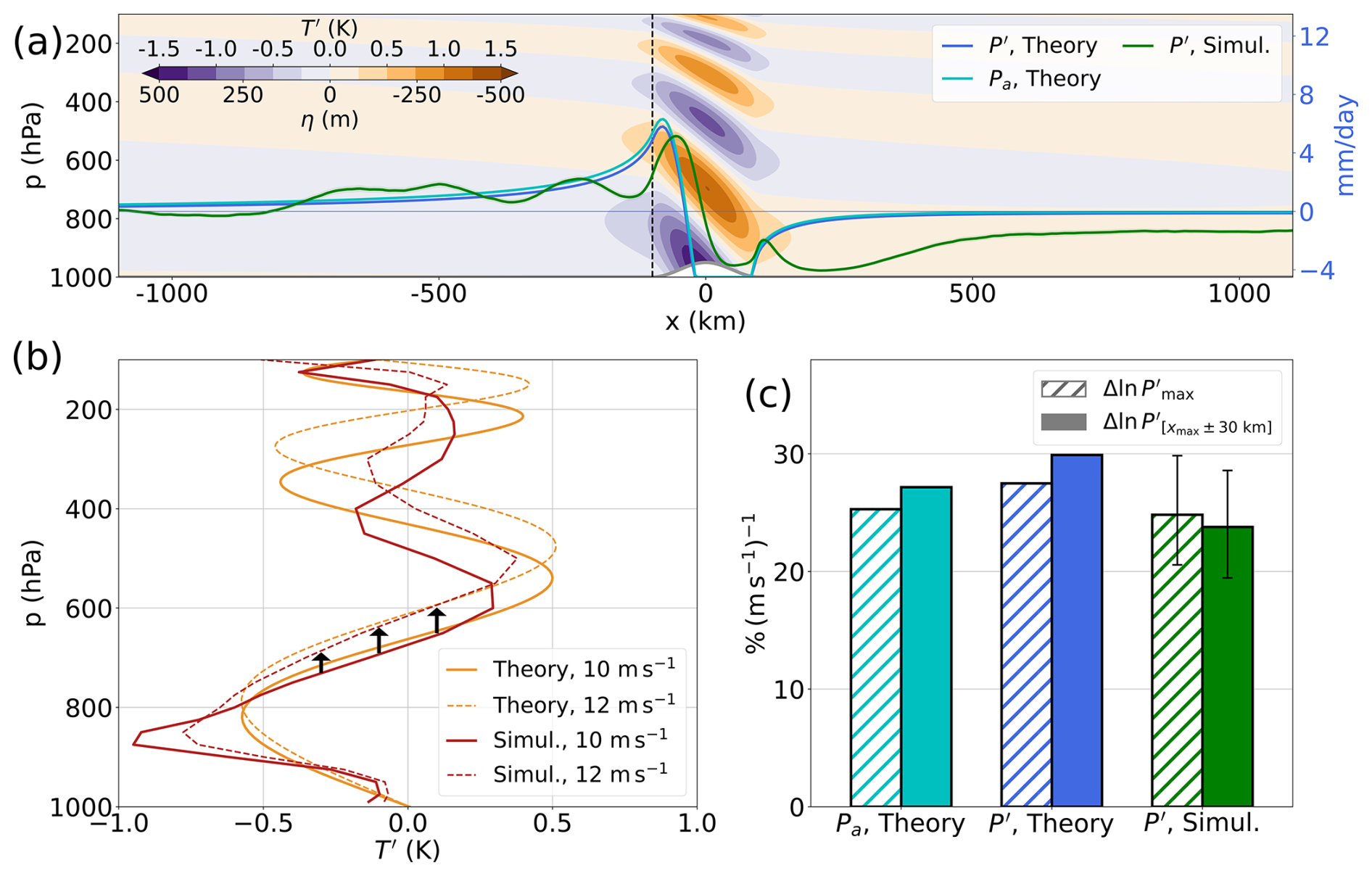
Figure 1 Orographic perturbations of temperature and precipitation in linear theory and a convection-permitting model, with sensitivities to wind speed. (a) Temperature perturbation T_a(x,p) in a stationary linear mountain wave with uniform static stability N = 0.01 s⁻¹ and cross-slope wind U = 10 m s⁻¹, for a 500 m mountain (color shading), precipitation perturbation P^′ = $max(P_a+P_m,-P_{\mathrm{0}})$ from the linear theory (dark-blue line; Eqs. 2 and 3), and the component of P^′ due to the adiabatic mountain wave alone P_a (cyan line). P^′ in a convection-permitting simulation (see text) is shown in green. The gray line shows surface height. T_a is proportional to the vertical displacement η(x,p) in the mountain wave, with scale shown at the bottom of the color bar. (b) Vertical structure of temperature perturbations at x = −100 km in the theory (orange) and simulations (red), with U = 10 m s⁻¹ (solid) and 12 m s⁻¹ (dashed). Arrows indicate the vertical stretching of the orographic gravity wave with increased wind. (c) Fractional increase in the maximum precipitation perturbation (hatched bars) and the precipitation perturbation averaged within 30 km of the maximum (solid), in the linear theory with and without convective feedback and in the simulations. Simulation results display a 95 % confidence interval (obtained by block bootstrapping, using 20 d blocks).

Convection feeds back on these perturbations, modifying the precipitation given by Eq. (2). For example, enhanced precipitating convection upstream of orography (P_a > 0) heats and dries the troposphere, thereby weakening the cool and moist lower-tropospheric perturbation. The system can be closed using conservation of dry static energy and moisture with other constraints from tropical dynamics (Nicolas and Boos, 2022), yielding a secondary precipitation perturbation P_m, obeying

$$\begin{array}{}\text{(3)}& {\displaystyle \frac{\mathrm{d}{P}_m}{\mathrm{d}x}}+{\displaystyle \frac{P_m+P_a}{L_q}}=\mathrm{0},\end{array}$$

where L_q is a length scale for the relaxation of lower-free-tropospheric moisture by convection (Appendix A). For U = 10 m s⁻¹, L_q ≃ 3000 km, which is large compared with the horizontal length scale l–100 km of the orographic forcing. Thus, scaling $\mathrm{d}{P}_m/\mathrm{d}x\sim P_m/l$, we expect P_m ∼ $-P_a/(\mathrm{1}+L_q/l)\ll P_a$.

For an idealized mountain of peak height 500 m, the solutions (Appendix A) feature a broad orographic enhancement of precipitation upstream of the mountain (Fig. 1a), peaking around 5 mm d⁻¹ on the upwind slope. The total precipitation anomaly $P^{\prime }=P_a+P_m$ is only about 10 % smaller there than the anomaly P_a that neglects convective feedback on the gravity wave, confirming the small damping effect of the feedback. A rain shadow extends downstream of the ridge, and negative precipitation values are prevented by enforcing P^′ ≥ −P₀, where we take P₀ = 4.5 mm d⁻¹ to conform with simulations presented below.

The sensitivity of P^′ to the background wind speed U arises through the vertical structure of η upstream of the mountain, which is wave-like with wavelength ${\mathit{\lambda }}_z=\mathrm{2}\mathit{\pi }U/N$ (Fig. 1a). Unlike its wavelength, the amplitude of η does not change with U, because it is set by the surface boundary condition η=h. In the linear theory (Eq. 2), η is proportional to −T_a; we thus expect the vertical structure of the gravity-wave-induced temperature anomaly to change with U while the amplitude remains constant. In order to later compare results with simulations (for which temperature perturbations are more readily available than η), we show the vertical structure of T_a in Fig. 1b (solid orange line). An increase in U (dashed orange line) results in deeper penetration of the ascending region of the wave (where T_a < 0), which amplifies T_aL upstream of orography. Similarly, q_aL is amplified by the same amount. With Eq. (2), this produces an increase in P_a and, because the convective feedback P_m is modest, also in P^′. We note that while the background moisture profile, especially the value of $\mathrm{d}{q}_{\mathrm{0}}/\mathrm{d}z$ in the lower free troposphere, sets P^′ by influencing q_aL (see Eq. 2), it has little influence on the relative sensitivity $\partial \ln P^{\prime }/\partial U$. Indeed, from Eq. (2), $\partial \ln P_a/\partial U=\partial \ln {\mathit{\eta }}_{\mathrm{L}}/\partial U$, an expression in which the moisture lapse rate does not appear because it does not depend on U. The background moisture profile does slightly affect the sensitivity of P^′ to U through its effect on the gross moist stability, which influences how P_m varies with U.

The precipitation increase produced by an increase in background wind U is quantified in Fig. 1c using two metrics: the maximum precipitation perturbation $P_{max}^{\prime }$ and the precipitation perturbation averaged within 30 km of the maximum $P_{[xmax\pm \mathrm{30}\mathrm{km}]}^{\prime }$. When U increases from 10 to 12 m s⁻¹, these quantities, respectively, increase by 27 % (m s⁻¹)⁻¹ and 30 % (m s⁻¹)⁻¹. Most of these increases (25 % (m s⁻¹)⁻¹ and 27 % (m s⁻¹)⁻¹) are explained by changes in P_a. This is a large sensitivity compared with the 10 % (m s⁻¹)⁻¹ expected from simple upslope flow considerations (see Introduction). Here, the increase stems from deeper vertical penetration of orographic ascent resulting in a stronger upstream cool and moist lower-tropospheric anomaly, in turn yielding a stronger precipitation anomaly. These sensitivities exhibit little dependence on convective timescales: halving or doubling them changes the sensitivities by less than 2 percentage points. However, sensitivities vary strongly with the levels used to define the lower free troposphere: lowering its top to 650 hPa from 600 hPa changes the sensitivity of $P_{max}^{\prime }$ to 19 % (m s⁻¹)⁻¹, while raising its top to 550 hPa yields 34 % (m s⁻¹)⁻¹. Using a convective closure that depends more continuously on thermodynamic perturbations at different levels (e.g., Kuang, 2010) may offer an avenue of improvement, at the expense of conceptual simplicity. Next, we use convection-permitting simulations and observations to validate these theoretical sensitivities.

3 Sensitivity in idealized simulations

3.1 Model setup

Our model setup is very similar to that used in Nicolas and Boos (2022) and is described here succinctly. We use the Weather Research and Forecasting model (WRF-ARW, version 4.1.5, Skamarock et al., 2019) to represent a doubly periodic long channel (9810 km wide in x by 198 km in y), with a y invariant 500 m high mountain identical to that used in the theory. The 3 km horizontal grid spacing and 60 terrain-following vertical levels (spanning from the surface to 10 hPa) are used to represent deep convective clouds without a convective parameterization. The domain is ocean-covered with a fixed SST of 300 K, except over the mountain where we employ the Noah-MP land surface scheme (Niu et al., 2011; Yang et al., 2011), with a no-flux bottom boundary condition. We fix the Coriolis parameter at 20° latitude and prescribe a constant background meridional pressure gradient which maintains a uniform background geostrophic zonal wind with speed U. We use a state of perpetual equinox (with a diurnal cycle) and calculate radiation interactively every hour using the RRTMG scheme (Iacono et al., 2008). Turbulent fluxes are calculated diffusively with a fixed horizontal diffusion of 300 m⁻² s⁻¹ and vertical diffusion of 100 m⁻² s⁻¹, with the Mellor–Yamada–Janjić scheme (Mellor and Yamada, 1982; Janjić, 2002) used for boundary layer fluxes. We use the Thompson scheme for microphysics (Thompson et al., 2008). Each simulation is run for 1000 d, after discarding 250 d of spinup. This long spinup time is required for the temperature profile to fully equilibrate in the stratosphere. Beyond 250 d, the simulations are in a quasi-steady state.

3.2 Changes in precipitation and free-tropospheric thermodynamic perturbations

We run two simulations, which only differ in background winds: one has U = 10 m s⁻¹ and the other U =12 m s⁻¹. In the 10 m s⁻¹ run, P^′ (Fig. 1a, green line) has numerous similarities with the theory, especially the peak precipitation rate and length scale of upstream orographic enhancement. Peak rainfall in the theory is shifted ∼ 25 km upstream compared to the simulations, a defect attributable to the convective closure: using Eq. (1) to diagnose P^′ with temperature and moisture perturbations from the simulations, instead of from a linear gravity wave solution, results in a similar shift (Fig. 2a). One reason for this upstream bias is the theory's vertically uniform dependence of rainfall on T and q perturbations in the lower free troposphere: giving higher weight to lower levels would shift the rainfall maximum downstream because maxima in T and q perturbations shift downstream at lower levels (Fig. 1a). Stronger differences appear between the theoretical and simulated P^′ downstream of the mountain, which we show below is due to neglect of θ_eB variations in our simplest scaling.

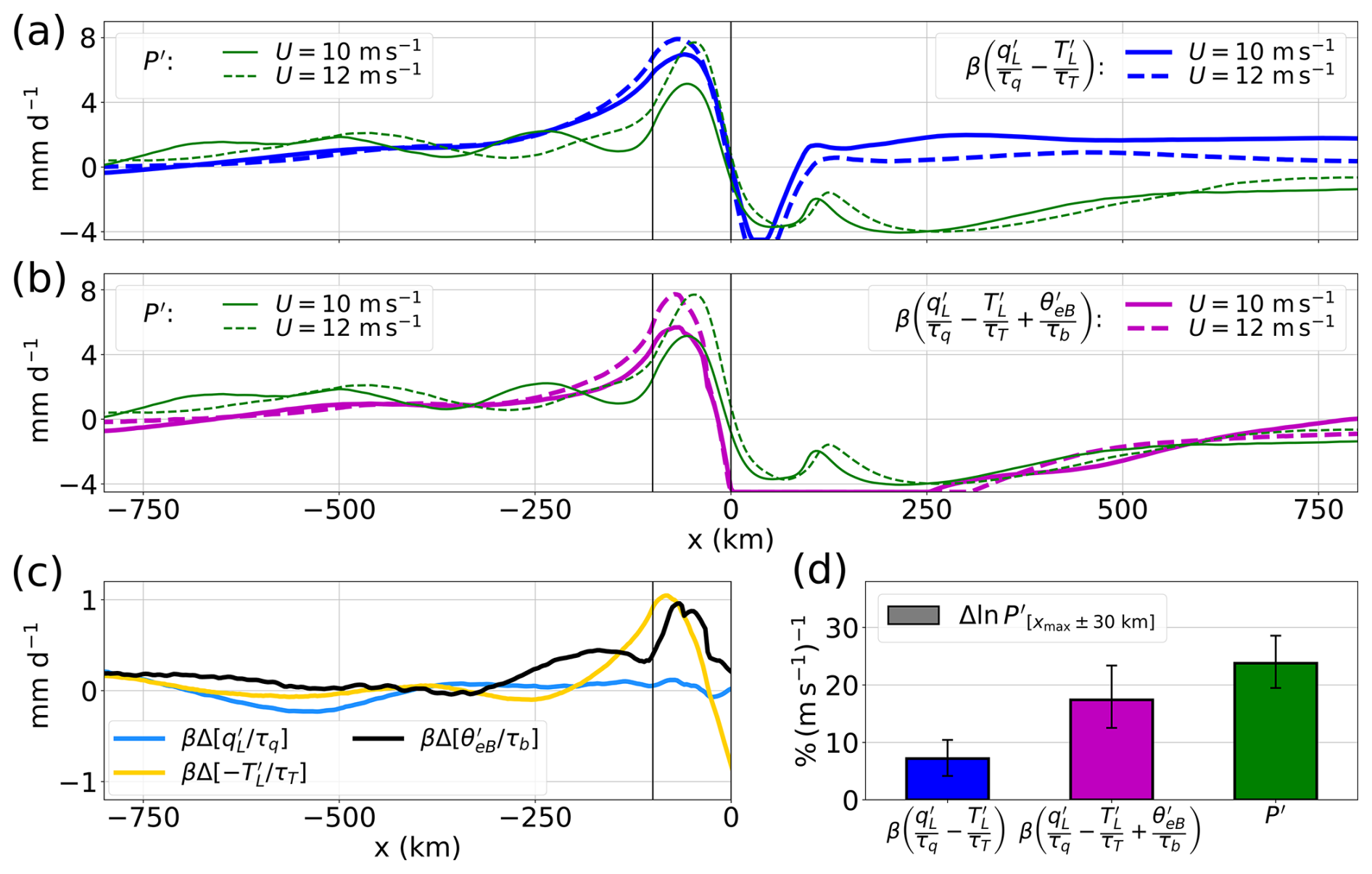
Figure 2 Drivers of the response of orographic precipitation to wind changes in convection-permitting simulations. (a) Mean precipitation perturbation P^′ for the two simulations (U = 10 m s⁻¹ and U = 12 m s⁻¹, green lines) and an estimate of P^′ by a version of the buoyancy-based closure (Eq. 1) that only considers T_L and q_L perturbations, clipped to eliminate negative total precipitation (blue lines). (b) As in panel (a) except using the full buoyancy-based closure (Eq. 1), shown as magenta lines. (c) Changes with increased wind in the three thermodynamic quantities in the buoyancy-based closure: lower-free-tropospheric moisture (blue), lower-free-tropospheric temperature (yellow), and boundary layer equivalent potential temperature (black). Each quantity is divided by its corresponding timescale from the convective closure. (d) Sensitivity of the precipitation perturbation averaged within 30 km of its maximum (green bar) and estimates of this using the two versions of the convective closure. We show 95 % confidence intervals (obtained by block bootstrapping, using 20 d blocks) for each sensitivity estimate. In panels (a)–(c), vertical black lines mark the mountain's upstream boundary and peak.

Both $P_{max}^{\prime }$ and $P_{[xmax\pm \mathrm{30}\mathrm{km}]}^{\prime }$ increase between 20 % (m s⁻¹)⁻¹ and 30 % (m s⁻¹)⁻¹ between the two simulations, commensurate with the theoretical prediction (Fig. 1c). Is this increase attributable to a deeper penetration of the stationary gravity wave cooling and moistening the lower free troposphere at higher U, as our theory suggests? To assess this we evaluate $T^{\prime }(x=-\mathrm{100}\mathrm{km},p)$ in both runs (Fig. 1b, red lines), where the reference profile is averaged over $x\in (-\mathrm{4000}\mathrm{km},-\mathrm{2500}\mathrm{km})$. T^′ displays a gravity wave structure in many ways similar to that of the adiabatic, linear T^′. With increased wind, the cool perturbation penetrates deeper (shown by black arrows in Fig. 1b), making $T_{\mathrm{L}}^{\prime }$ more negative. While quantitative differences with the theory's T^′ arise because static stability is not vertically uniform in the simulations, the change in T^′ with increased wind is well captured by linear theory.

To assess whether this deepening of the T^′ structure, with the accompanying changes in q^′, can quantitatively explain the increase in P^′, we compute precipitation from the linear closure used in our theory: $P_{qT}^{\prime }=\mathit{\beta }\left(q_{\mathrm{L}}^{\prime }/{\mathit{\tau }}_q-T_{\mathrm{L}}^{\prime }/{\mathit{\tau }}_{\mathrm{T}}\right)$ (Fig. 2a, blue lines). This diagnostic captures the magnitude of the simulated precipitation peak for U = 12 m s⁻¹ with a similar upstream shift to the theory, but it shows a dependence on U that is too weak. Specifically, the change in upstream $P_{qT}^{\prime }$ (averaged within 30 km of its maximum) between both simulations is only 7 % (m s⁻¹)⁻¹ (Fig. 2d, blue bar), indicating that the increase in peak precipitation with increased wind is only partly attributable to stronger lower-tropospheric T and q perturbations.

3.3 Changes in boundary layer moist entropy

We now show that this discrepancy can be resolved by considering variations in θ_eB and that these variations are controlled by the same mountain wave dynamics discussed earlier. Using ${\mathit{\theta }}_{\mathrm{eB}}^{\prime }$ in conjunction with $T_{\mathrm{L}}^{\prime }$ and $q_{\mathrm{L}}^{\prime }$ (all diagnosed from simulations) in Eq. (1) generally improves comparison to the simulated P^′, better fitting upstream rain rates and the rain shadow (Fig. 2b, magenta lines). The value of this diagnosed precipitation, $\mathit{\beta }\left(q_{\mathrm{L}}^{\prime }/{\mathit{\tau }}_q-T_{\mathrm{L}}^{\prime }/{\mathit{\tau }}_{\mathrm{T}}+{\mathit{\theta }}_{\mathrm{eB}}^{\prime }/{\mathit{\tau }}_b\right)$, still averaged within 30 km of its maximum, increases by 17 % (m s⁻¹)⁻¹, a value much closer to the 24 % (m s⁻¹)⁻¹ change in simulated P^′ (95 % confidence intervals on these two values overlap; Fig. 2d). The increases in ${\mathit{\theta }}_{\mathrm{eB}}^{\prime }$ and in the magnitude of $T_{\mathrm{L}}^{\prime }$, induced by the change in U, contribute similarly to the increase in the P^′ maximum, while changes in $q_{\mathrm{L}}^{\prime }$ contribute negligibly (Fig. 2c). Thus, the quantitative match between theoretical and simulated precipitation changes in Fig. 1c appears in part fortuitous: while moistening of the lower free troposphere with increased wind is important in setting the sensitivity of P^′ in the theory, no such moistening occurs in simulations. Half of the sensitivity exhibited by the simulations is explained by an increase in ${\mathit{\theta }}_{\mathrm{eB}}^{\prime }$, an effect not represented by the theory. We examine the reason for the stagnation in $q_{\mathrm{L}}^{\prime }$ between simulations in the next subsection.

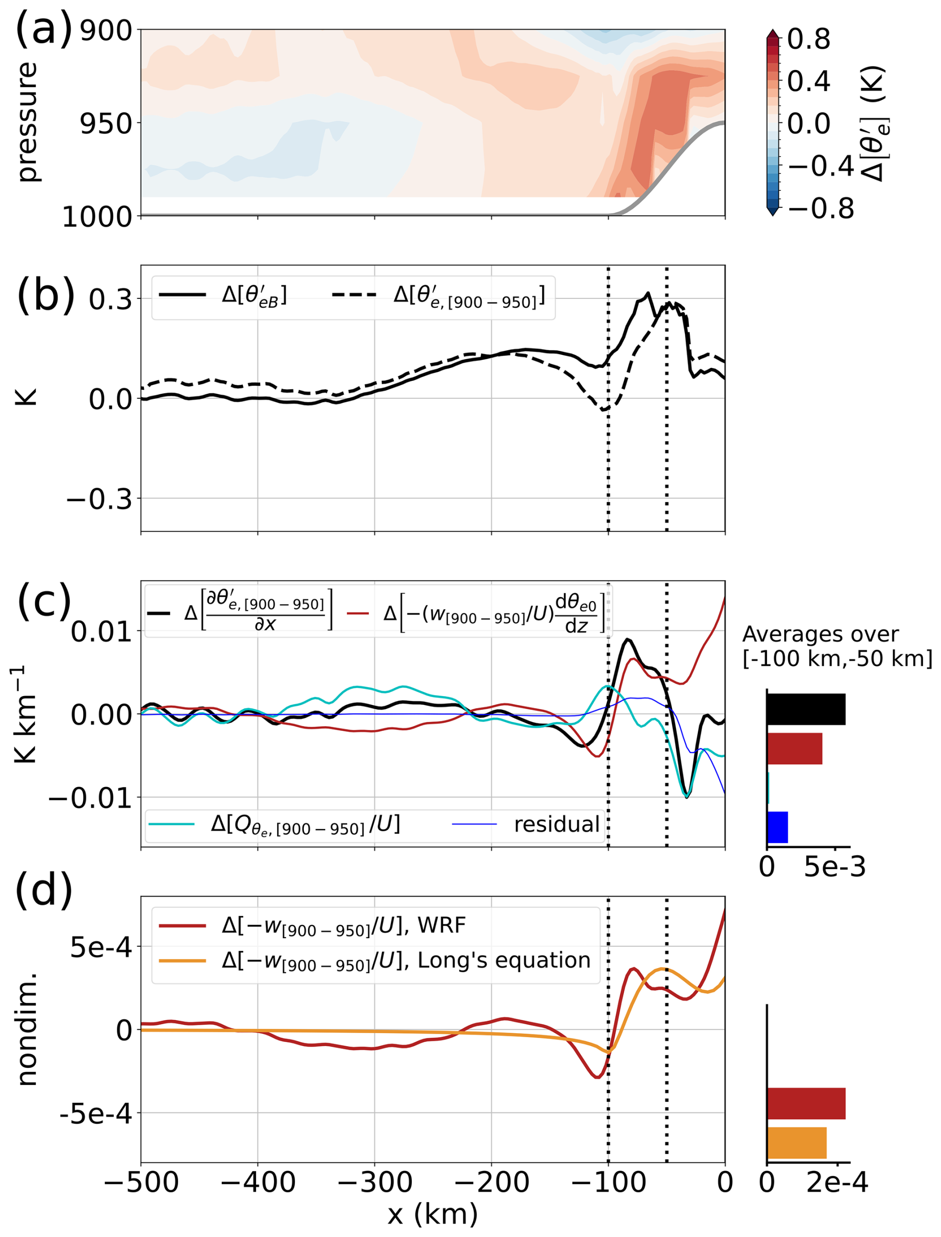
Figure 3 ${\mathit{\theta }}_{\mathrm{eB}}^{\prime }$ variations between the 10 and 12 m s⁻¹ simulations and their physical drivers. Throughout the figure, $\mathrm{\Delta }[\cdot ]\equiv [\cdot {]}_{\mathrm{12}\mathrm{m}{\mathrm{s}}^{-\mathrm{1}}}-[\cdot {]}_{\mathrm{10}\mathrm{m}{\mathrm{s}}^{-\mathrm{1}}}$. (a) $\mathrm{\Delta }\left[{\mathit{\theta }}_e^{\prime }\right]$ in the boundary layer (shading). The thick gray line shows the topography. (b) $\mathrm{\Delta }\left[{\mathit{\theta }}_{\mathrm{eB}}^{\prime }\right]$ (solid) and $\mathrm{\Delta }\left[{\mathit{\theta }}_e^{\prime }\right]$ averaged between 900 and 950 hPa (dashed). Note the qualitative similarity between the two profiles upstream of the mountain, with a rapid increase over the upwind slope. (c) Differential budget of ${\mathit{\theta }}_e^{\prime }$ averaged over [900 hPa, 950 hPa] between the two runs. Differences in horizontal gradients of ${\mathit{\theta }}_e^{\prime }$ (black) are balanced by differences in vertical advection divided by U (red line) and differences in diabatic sources divided by U (cyan line). The residual is shown as a thin blue line. Note the sharp peak in the black line above the mountain's upwind slope, mostly contributed to by changes in vertical advection. A bar plot shows averages of each term in the $x\in (-\mathrm{100}\mathrm{km},-\mathrm{50}\mathrm{km})$ region, where the large increase in $\mathrm{\Delta }\left[{\mathit{\theta }}_{\mathrm{eB}}^{\prime }\right]$ occurs. (d) Change in ascent slope $w/U$ between the two runs, as diagnosed from simulations (red line) and from a nonlinear theory (orange line; see text). As in panel (c), a bar plot shows averages of each term in the $x\in (-\mathrm{100}\mathrm{km},-\mathrm{50}\mathrm{km})$ region. In panels (c) and (d), all terms from simulations are smoothed with a Gaussian filter of standard deviation of 6 km to filter out small-scale noise. In all panels, vertical dotted lines show the upstream boundary of the mountain (x = −100 km) and the x = −50 km location.

We proceed to show that the increase in ${\mathit{\theta }}_{\mathrm{eB}}^{\prime }$ with increased wind can also be attributed to the vertical stretching of the orographic ascent pattern that occurs with increasing U. The difference (denoted by a Δ) between boundary layer ${\mathit{\theta }}_e^{\prime }$ in the 12 and 10 m s⁻¹ runs is shown in Fig. 3a, with its mass-weighted vertical average $\mathrm{\Delta }\left[{\mathit{\theta }}_{\mathrm{eB}}^{\prime }\right]$ shown in Fig. 3b (solid black). ${\mathit{\theta }}_{\mathrm{eB}}^{\prime }$ is about 0.3 K warmer over the upwind slope with increased wind. In order to understand this increase, we diagnose the ${\mathit{\theta }}_e^{\prime }$ budget over a subset of pressure levels which do not cross the topography, namely 900–950 hPa. Averaged over these levels, $\mathrm{\Delta }\left[{\mathit{\theta }}_e^{\prime }\right]$ has a qualitatively similar structure to $\mathrm{\Delta }\left[{\mathit{\theta }}_{\mathrm{eB}}^{\prime }\right]$ upstream of the mountain peak (Fig. 3b), with modest variations for x < −100 km and a rapid increase from x = −100 km to x = −50 km.

The time-averaged, meridionally averaged ${\mathit{\theta }}_e^{\prime }$ budget can be written

$$\begin{array}{}\text{(4)}& u{\displaystyle \frac{\partial {\mathit{\theta }}_e^{\prime }}{\partial x}}+w{\displaystyle \frac{\partial {\mathit{\theta }}_e}{\partial z}}=Q_{{\mathit{\theta }}_e},\end{array}$$

where all quantities are time and meridional means, and $Q_{{\mathit{\theta }}_e}$ is an apparent source of θ_e due to transients, meridional fluctuations, and diabatic sources (in the boundary layer, its main contributors are surface fluxes, turbulent mixing, and penetrative downdrafts). We evaluate the two terms on the left-hand side from temporally and meridionally averaged u, w, and θ_e fields and compute $Q_{{\mathit{\theta }}_e}$ as a residual.

An approximate version of Eq. (4), which is valid upstream of the ridge top (see residual term in Fig. 3c), is

$$\begin{array}{}\text{(5)}& U{\displaystyle \frac{\partial {\mathit{\theta }}_e^{\prime }}{\partial x}}+w{\displaystyle \frac{\mathrm{d}{\mathit{\theta }}_{e\mathrm{0}}}{\mathrm{d}z}}\simeq Q_{{\mathit{\theta }}_e},\end{array}$$

where $\mathrm{d}{\mathit{\theta }}_{e\mathrm{0}}/\mathrm{d}z$ is a horizontally invariant lapse rate of θ_e, averaged 2500–4000 km upstream of the mountain ($\mathrm{d}{\mathit{\theta }}_{e\mathrm{0}}/\mathrm{d}z$ = −19.8 K km⁻¹ at 925 hPa). In this approximation, variations in vertical advection are controlled by w, while variations in horizontal advection are controlled by the imposed background wind U and horizontal ${\mathit{\theta }}_e^{\prime }$ gradients. Over the mountain, we expect w to be controlled by mountain wave dynamics and $Q_{{\mathit{\theta }}_e}$ by convective processes, while $\partial {\mathit{\theta }}_e^{\prime }/\partial x$ adjusts to balance the budget given by Eq. (5). Thus, we reorganize Eq. (5) to

$$\begin{array}{}\text{(6)}& {\displaystyle \frac{\partial {\mathit{\theta }}_e^{\prime }}{\partial x}}\simeq -{\displaystyle \frac{w}{U}}{\displaystyle \frac{\mathrm{d}{\mathit{\theta }}_{e\mathrm{0}}}{\mathrm{d}z}}+{\displaystyle \frac{Q_{{\mathit{\theta }}_e}}{U}}\end{array}$$

and show the difference (denoted by Δ) in each terms in Eq. (6) between the 12 and 10 m s⁻¹ runs, averaged over 900–950 hPa (Fig. 3c). Because Eq. (6) is approximate, we show the residual term, which is due to horizontal variations in u and $\partial {\mathit{\theta }}_e/\partial z$ and is small upstream of the ridge top. Over the ocean part of the domain (x < −100 km), horizontal gradients in ${\mathit{\theta }}_e^{\prime }$ are constrained to be small by the uniform SST. Hence, $\mathrm{\Delta }[\partial {\mathit{\theta }}_e^{\prime }/\partial x]$ is small there. Over the mountain, the increase in $\mathrm{\Delta }{\mathit{\theta }}_e^{\prime }$ seen in Fig. 3b translates into a large peak in $\mathrm{\Delta }[\partial {\mathit{\theta }}_e^{\prime }/\partial x]$ around $x\in (-\mathrm{100}\mathrm{km},-\mathrm{50}\mathrm{km})$. Importantly, most of this peak is associated with the change in vertical advection normalized by U (red line; see also the bar plot on the right side of Fig. 3c). In other words, vertical advection increases faster than U, while diabatic sources increase at a rate close to U. An increase in $\partial {\mathit{\theta }}_e^{\prime }/\partial x$ maintains the balance given by Eq. (5) and leads to a positive anomaly in ${\mathit{\theta }}_{\mathrm{eB}}^{\prime }$ over the mountain.

We now argue that this change in vertical advection is explained by the same deepening of the mountain wave discussed earlier. This is illustrated in Fig. 4 (red lines), where we show vertical profiles of $w/U$ over the mountain's upwind slope in simulations. While the surface value of $w/U$ changes little, consistent with linear theory, its profile stretches vertically with increased U, leading to an increase in $w/U$ averaged over the boundary layer. Can this change be captured by mountain wave theory? To answer this question, we solve for the mountain wave using Long's equation (Long, 1953), as linearization of the boundary condition in classical linear mountain wave theory yields inaccuracies in the boundary layer. Neglecting damping, the vertical displacement η satisfies

$$\begin{array}{}\text{(7)}& {\partial }_{zz}\mathit{\eta }+{\displaystyle \frac{N^{\mathrm{2}}}{U^{\mathrm{2}}}}\mathit{\eta }=\mathrm{0},\mathit{\eta }(z=h(x\left)\right)=h\left(x\right),\end{array}$$

with a radiation upper boundary condition. We solve Eq. (7) using an iterative procedure (Lilly and Klemp, 1979) and obtain w as $U\partial \mathit{\eta }/\partial x$ (orange lines in Fig. 4). While this theory overestimates the magnitude of $w/U$ (this happens in the boundary layer because the theory does not include surface friction), it features a similar vertical stretching of $w/U$ when U increases, as in the simulations. Figure 3d confirms that the theory captures the change in $w/U$ in the boundary layer with good quantitative accuracy. This agreement indicates that mountain wave dynamics explain the stronger boundary layer ${\mathit{\theta }}_e^{\prime }$ perturbation and, ultimately, the stronger rainfall peak with increased U.

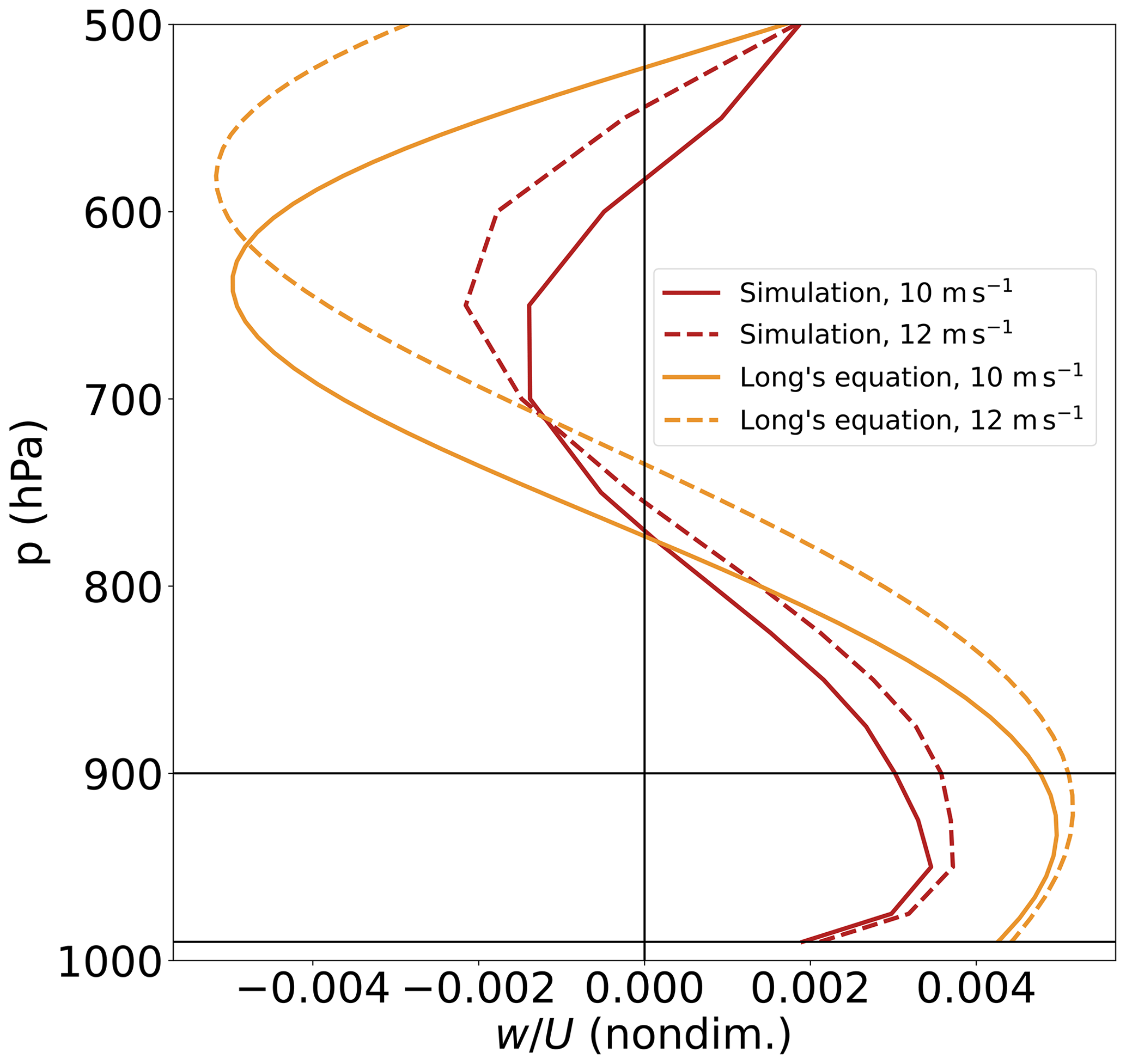
Figure 4 Vertical profiles of vertical velocity normalized by the background wind U, over the upwind slope (x = −75 km), for U = 10 m s⁻¹ (solid lines) and U = 12 m s⁻¹ (dashed lines). Red lines show time averages from simulations, and orange lines are from a nonlinear theory (see text).

3.4 Free-tropospheric humidity sensitivity to U

We now explain how an enhanced convective moisture sink prevents $q_{\mathrm{L}}^{\prime }$ from increasing with U in the simulations, even though it was predicted to increase by the simple theory. Recalling the argument made in Sect. 2 for the changes in T_aL and q_aL produced by increased U, we expect q_a $=-\mathit{\eta }\mathrm{d}{q}_{\mathrm{0}}/\mathrm{d}z$ so that vertical stretching of the mountain wave induces an increase in η_L and thus an increase in q_aL. Equivalently, since ${\partial }_x\mathit{\eta }=w/U$, one may write $\partial q_a/\partial x=-(w/U)\mathrm{d}{q}_{\mathrm{0}}/\mathrm{d}z$, where w is the adiabatic mountain wave vertical velocity. Deepening of the mountain wave is thus expected to increase $w/U$ in the lower free troposphere, increasing horizontal q_a gradients, hence increasing q_a. So why does $q_{\mathrm{L}}^{\prime }$ not increase with U in simulations (e.g., blue line in Fig. 2c)? As we did in Eq. (6), we obtain an equation for the horizontal q^′ gradient:

$$\begin{array}{}\text{(8)}& {\displaystyle \frac{\partial q^{\prime }}{\partial x}}\simeq -{\displaystyle \frac{w}{U}}{\displaystyle \frac{\mathrm{d}{q}_{\mathrm{0}}}{\mathrm{d}z}}+{\displaystyle \frac{Q_q}{U}},\end{array}$$

where Q_q is an apparent source of moisture due to convection (in regions of enhanced convection, Q_q is negative in the lower troposphere). Figure 5 shows, for each term in Eq. (8), the difference between the 12 and 10 m s⁻¹ runs averaged over the lower free troposphere. While differences in vertical advection normalized by U do act to increase $\partial q^{\prime }/\partial x$ between about −200 km and the mountain peak (red line), they are counterbalanced by an increased convective moisture sink (cyan line) so that $\mathrm{\Delta }\left[\partial q^{\prime }/\partial x\right]$ ≃ 0, and $q_{\mathrm{L}}^{\prime }$ stays nearly unchanged between simulations. The theory does contain a convective moisture sink (leading to the P_m term in Eq. 3), but its changes with U are much weaker than those seen in the simulations.

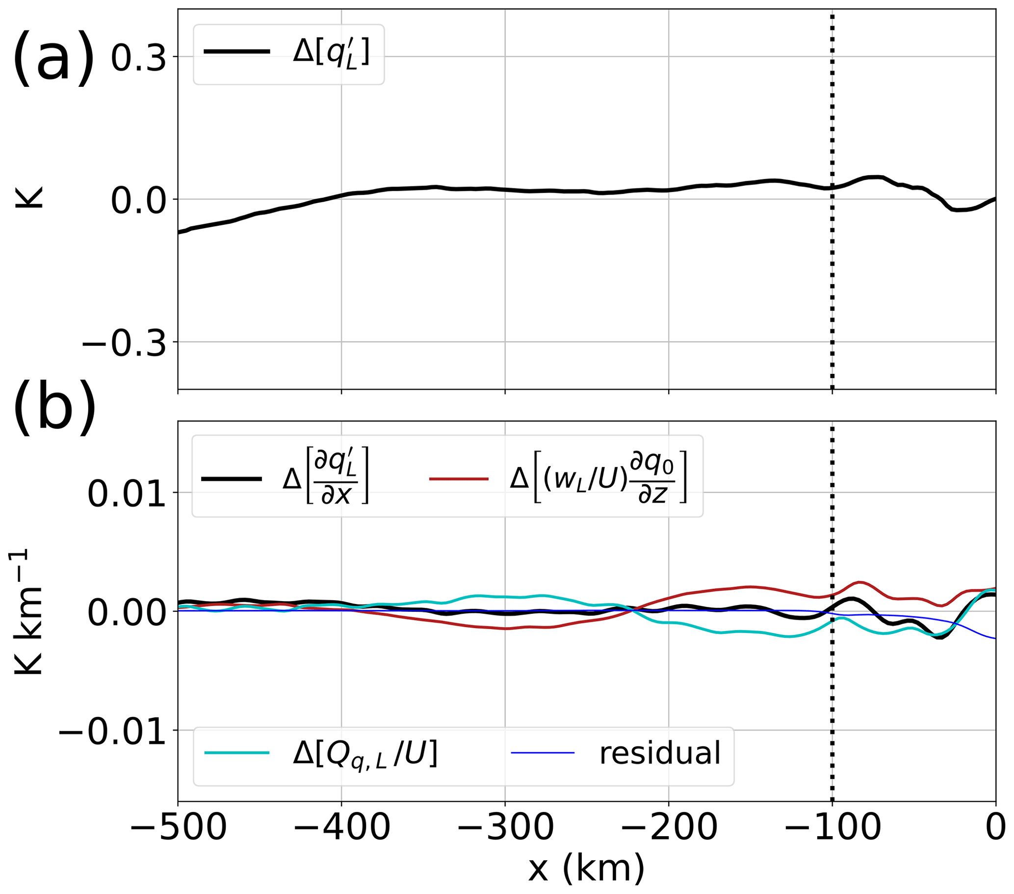
Figure 5 Lower-free-tropospheric moisture variations between the 10 and 12 m s⁻¹ simulations and their physical drivers. Throughout the figure, $\mathrm{\Delta }[\cdot ]\equiv [\cdot {]}_{\mathrm{12}\mathrm{m}{\mathrm{s}}^{-\mathrm{1}}}-[\cdot {]}_{\mathrm{10}\mathrm{m}{\mathrm{s}}^{-\mathrm{1}}}$. (a) $\mathrm{\Delta }\left[q_{\mathrm{L}}^{\prime }\right]$; note the relatively flat profile upstream of the mountain. (b) Differential budget of $q_{\mathrm{L}}^{\prime }$ between the two runs. Differences in horizontal gradients of $q_{\mathrm{L}}^{\prime }$ (black) are balanced by differences in vertical advection divided by U (red line) and differences in the convective source divided by U (cyan line). The residual is shown as a thin blue line. All terms are smoothed with a Gaussian filter of standard deviation of 6 km to filter out small-scale noise. In both panels, a vertical dotted line indicates the upstream boundary of the mountain. The y-axis ranges are the same as in Fig. 3b–c, for ease of comparison.

4 Observed sensitivity at various timescales

Do observations support the above theoretical and model-derived sensitivities? The framework developed in this work quantifies changes in the seasonal mean orographic precipitation perturbation $P^{\prime }=P-P_{\mathrm{0}}$, where P and P₀ are the total and background precipitation rates, respectively. We now aim to evaluate the observed dependence of P^′ on variations in the background cross-slope wind U in five tropical orographic regions, recognizing that changes in U may also be associated with changes in P₀. All the orographic regions we consider lie downstream of an ocean, over which rainfall observations at the fine spatial scales needed here are only available for the past 2 decades. Therefore, because P₀ is 3–5 times smaller than P^′ in three of our regions, we first neglect P₀ and estimate the sensitivity of seasonal mean P to interannual changes in seasonal mean U using gridded gauge-based rainfall observations. We then estimate the sensitivity of P^′ to U on two different timescales using two rainfall products: satellite-estimated precipitation for daily variations in 2001–2020 and reanalysis-derived precipitation for interannual variations in 1960–2015 (see Appendix B for more details). These two approaches come with two caveats: one may question whether daily mean P^′ scales similarly to seasonal mean P^′ with changes in U,¹ and reanalysis precipitation has few observational constraints prior to 1979. Nevertheless, the estimated sensitivities prove to be consistent across regions and timescales.

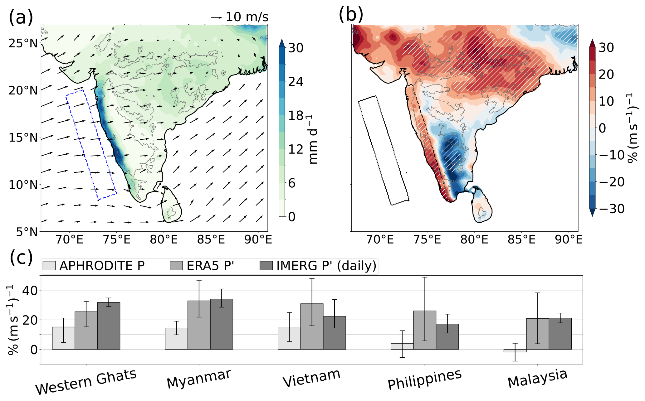
Figure 6 Evidence for large precipitation scaling rates from observational and reanalysis data at multiple timescales. (a) Observed summer mean (June–August, 1960–2015) precipitation over India and 100 m winds from reanalysis. Gray contours mark 500 m surface height. (b) Sensitivity of summer mean precipitation to cross-slope wind speed upstream of the Western Ghats. Regions hatched in white satisfy the false-discovery-rate criterion (Wilks, 2016) with α=0.1. Winds are averaged in the dashed blue rectangle shown in panel (a). (c) Sensitivity of orographic precipitation P and precipitation perturbation $P^{\prime }=P-P_{\mathrm{0}}$ to upstream cross-slope wind in multiple regions and at multiple timescales. In all cases, P is averaged in the peak rainfall region, and P₀ is averaged from 200 to 400 km upstream (dashed and solid black boxes, respectively, in panel (b) for the Western Ghats; see Fig. S1 for other regions). Light-gray bars show the sensitivity of observed seasonal mean P, medium-gray bars the sensitivity of seasonal mean P^′ from a reanalysis, and dark bars the sensitivity of daily observed P^′ over 2001–2020. A 95 % confidence interval obtained by bootstrapping is shown for each estimate.

We evaluate orographic rainfall variations in five regions of South and Southeast Asia: the west coasts of India and Myanmar and the east coasts of Vietnam, Malaysia, and the Philippines (see Appendix B and Fig. S1 in the Supplement for details on regions and seasons selected). In each region, the interaction of prevailing winds with a coastal mountain range creates a precipitation maximum over and upstream of the mountains (Nicolas and Boos, 2024). In the Western Ghats, for example, precipitation rates are 2–3 times higher than over the core monsoon region of central India (Fig. 6a). Seasonal mean cross-slope wind (defined as the projection along the 70° azimuthal angle, roughly east–northeast) is averaged upstream of the Western Ghats (over the blue rectangle in Fig. 6a). This yields a 56-year time series of cross-slope wind speed, on which we regress seasonal mean P (from a gridded gauge-based dataset; see Appendix B) over the Indian subcontinent. The resulting regression slopes are divided by P to obtain relative sensitivities, which exhibit a dipolar pattern in which the regions upstream of mountain peaks are positively associated with U, while regions in the orographic rain shadow exhibit negative sensitivity (Fig. 6b). A decrease in downstream precipitation with increased U is also visible in a 300 km wide region in the simulations (Fig. 2a). Rainfall also positively correlates with U across central India, consistent with the stronger diabatic heating of increased monsoon rainfall accompanying a stronger large-scale monsoon circulation (Rodwell and Hoskins, 2001). Absolute sensitivities over central India are, however, 2–3 times weaker than in the peak rainfall region upstream of the Western Ghats (i.e., the relative sensitivities are elevated over central India because P is comparatively small there).

Although it cannot be directly compared with our theoretical and model-derived sensitivities of P^′, we evaluate the sensitivity of spatially averaged P (in the orographic precipitation band marked by a dashed black line in Fig. 6b) to interannual wind changes. It scales at 15 % (m s⁻¹)⁻¹, with local values as high as 30 % (m s⁻¹)⁻¹. Figure 6c (light-gray bars) extends this analysis to four other regions. In Myanmar and Vietnam, where P₀ is much smaller than P^′, seasonal mean P exhibits a similar sensitivity to cross-slope wind to the Western Ghats (around 15 % (m s⁻¹)⁻¹). Sensitivities are much lower in the Philippines and Malaysia. We show in the Supplement (Fig. S2) that increased cross-slope winds in these two regions are associated with large-scale reductions in specific humidity. This suggests that increased U accompanies a general drying and perhaps a decrease in P₀ there. To test this hypothesis, we turn to other precipitation datasets that contain data over the ocean, allowing estimates of P₀ and thus P^′.

We use two rainfall datasets to estimate the observed sensitivity of P^′, which can be directly compared with our theoretical and model estimates. Reanalysis-estimated seasonal mean P^′ and satellite-estimated daily mean P^′ are obtained as the difference between P in the peak orographic rainfall region and P in a region 400 km upstream (dashed and solid black rectangles in Fig. 6b for the Western Ghats; see Fig. S1 for other regions). These P^′ values are regressed on upstream cross-slope wind at the corresponding seasonal or daily timescales. P^′ is strongly sensitive to changes in U at both seasonal and daily scales, with central estimates ranging from 17 % (m s⁻¹)⁻¹ to 34 % (m s⁻¹)⁻¹ across regions (Fig. 6c, medium-gray and dark-gray bars), in line with the theoretical and simulated sensitivities. While this analysis controls for variations in P₀, it does not control for potential changes in moisture stratification or static stability that may correlate with U (although Fig. S2 suggests such interannual changes are modest in most regions). Differences in climatological cross-slope wind between regions may be another source of interregional variability. However, all five regions exhibit strong sensitivities on both timescales that quantitatively agree with the 20 % (m s⁻¹)⁻¹ to 30 % (m s⁻¹)⁻¹ values seen in our theoretical and model estimates.

5 Discussion and implication for regional rainfall change

We have presented multiple lines of evidence indicating that tropical orographic rainfall maxima increase with cross-slope wind speed at a rate of 20 % (m s⁻¹)⁻¹–30 % (m s⁻¹)⁻¹. This rate is grounded in physically based theory, holds in a set of convection-permitting simulations, and is observed in several regions on multiple timescales. While the fact that mechanically forced orographic rainfall increases with wind speed is not surprising, the magnitude of this sensitivity has important implications for tropical rainfall projections.

Regional rainfall changes accompanying global warming have traditionally been understood from a thermodynamic standpoint, where an increase in specific humidity following the Clausius–Clapeyron (CC) rate of ∼ 7 % K⁻¹ implies a similar increase in the magnitude of precipitation minus evaporation (Held and Soden, 2006). This thermodynamic increase has become a null hypothesis for regional precipitation change, with deviations from the CC rate often attributed to changes in winds. Here, we presented a mechanism by which such changes in large-scale winds can affect regional precipitation.

To evaluate whether this mechanism may appreciably strengthen or offset any thermodynamic rainfall change, we evaluate cross-slope wind changes in our five regions in 37 models from the Coupled Model Intercomparison Project Phase 6 (CMIP6, Eyring et al., 2016; see Table S1 in the Supplement for the list of models). We evaluate wind changes between the end of the 20th century in historical simulations and the end of the 21st century in the high-emission SSP5-8.5 scenario.² Models agree on a weakening of ∼ 0.5 m s⁻¹ in cross-slope wind upstream of the Western Ghats, consistent with a general weakening of monsoon circulations with warming (Douville et al., 2021). Given our sensitivity estimate, this weakening would yield a 10 %–15 % decrease in the orographic precipitation anomaly P^′ or a 9 %–13 % in total precipitation P (assuming a fixed P₀ of 3 mm d⁻¹). This represents a sizable reduction of the “null-hypothesis” 27 % increase that may result from a CC scaling, assuming a 3.5 K surface warming in that region (Gutiérrez et al., 2023). In Myanmar, the Philippines, and Malaysia, models disagree on the sign of cross-slope wind changes, but the multi-model mean absolute wind changes remain substantial (0.3–0.5 m s⁻¹). This implies a potential for large changes in rainfall of either sign. In Vietnam, models agree on a more modest change in winds.

A purely thermodynamic change in orographic precipitation (i.e., one produced by climate warming with fixed cross-slope winds) may be smaller than the CC rate discussed above. In Eq. (2), mechanically forced orographic precipitation is set by the background moisture stratification, static stability, and orographic vertical displacement. The first of these likely increases with warming close to the CC rate. Tropical static stability also increases with warming, which strengthens T_aL and thus P_a; at the same time, however, this decreases vertical displacement by contracting the orographic gravity wave, weakening P_a. This may imply a smaller thermodynamic increase than the CC rate, possibly even an overall stagnation or decrease in total precipitation in some regions. Past studies have reached similar conclusions, albeit for different physical reasons, for midlatitude orographic precipitation (Kirshbaum and Smith, 2008; Shi and Durran, 2014; Koszuta et al., 2024).

It may be difficult to project future changes in tropical orographic rainfall using climate models because those models do not resolve orographic gravity waves or moist convection, two central processes in orographic precipitation. The width of the rainfall peaks in Fig. 6 is around 60 km, smaller than the grid scale of half the CMIP6 models analyzed here. We suggest that two components are in principle necessary to capture this rainfall distribution: a stationary orographic wave and the correct sensitivity of convection to temperature and moisture perturbations. The first component can be represented by models if topography and the gravity wave structure (e.g., Fig. 1a) can be resolved, which likely requires grid scales at or below 𝒪(10 km). Past work has evaluated the second component in CMIP6 models (Ahmed and Neelin, 2021), concluding that few models have adequate sensitivities. Furthermore, gravity wave parameterizations in climate models are typically used to provide drag in the upper troposphere–stratosphere and do not interact directly with model convection schemes. Theory, convection-permitting models, and observational analyses may thus be the primary tools with which orographic precipitation can be reliably projected.

Our analyses have several limitations. The theoretical sensitivity estimate depends on the definition of the lower-tropospheric layer used to define $T_{\mathrm{L}}^{\prime }$ and $q_{\mathrm{L}}^{\prime }$. There is uncertainty in the definition of its lower edge (the boundary layer top), and its upper boundary has been chosen somewhat arbitrarily here and in past related work (Nicolas and Boos, 2022; Ahmed et al., 2020). Using a vertically resolved sensitivity kernel (Kuang, 2010) may render the theory more robust. However, such kernels depend on the cloud-resolving model and simulation design used to derive it, and none have yet been estimated from observations. Our sensitivity estimate remains robust to changes in many other parameters of the theory.

Our simulations also have limitations, as convection-permitting models exhibit differences in emergent properties such as cloud entrainment rates and precipitation efficiencies (Wing and Singh, 2024). These might affect the sensitivity of convection to temperature and moisture perturbations and hence the scalings derived here. Another limitation is that we only considered one SST (300 K) in our simulations. Although it is representative of current conditions in most of the observed regions analyzed, different SSTs may alter the sensitivity of convection. Finally, our idealized simulations may oversimplify the large-scale conditions of observed orographic precipitation, neglecting spatial and temporal variations in background wind and SST.

Two important unknowns preclude a projection of tropical orographic precipitation in a warmer world. First, warming-induced changes in cross-slope wind are uncertain in many regions (Fig. 7). Second, away from midlatitudes (Siler and Roe, 2014), the sensitivity of orographic precipitation to warming with fixed wind remains unknown, even though it likely is the most important factor in regions where wind changes are modest. Progress constraining either of these quantities will help in anticipating changes in freshwater supplies for billions of people.

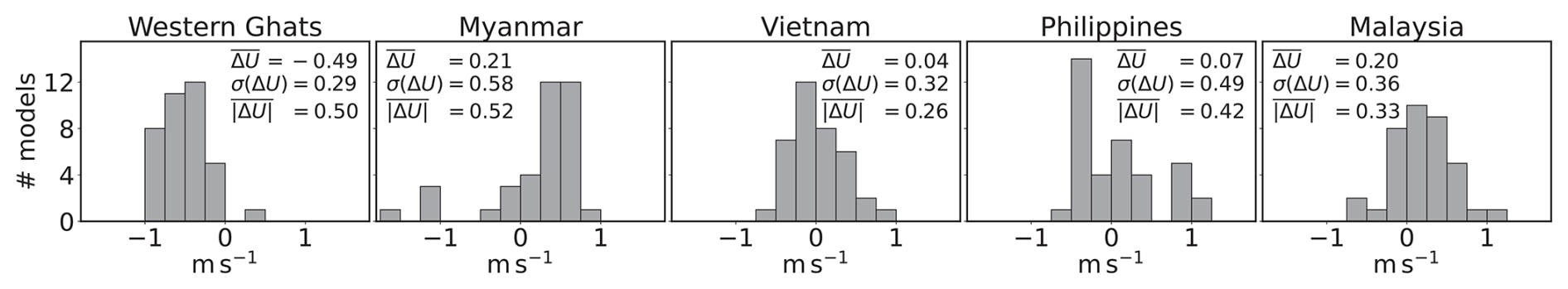
Figure 7 Distribution of cross-slope wind changes in CMIP6 climate models under a high-emission scenario. For each region and model, we take the difference between 10 m cross-slope wind, averaged in the same upstream region as in Fig. 6, between 2080–2099 (in the SSP5-8.5 scenario) and 1980–1999 (in the historical run). Results for 37 models are shown as histograms for each region, with the multi-model mean change $\stackrel{\mathrm{‾}}{\mathrm{\Delta }U}$, standard deviation σ(ΔU), and mean absolute change $\stackrel{\mathrm{‾}}{\left|\mathrm{\Delta }U\right|}$.

Appendix A: Linear theory for tropical orographic precipitation

Nicolas and Boos (2022) derive an equation for orographic precipitation in one horizontal dimension (their Eq. 7) which reads

$$\begin{array}{}\text{(A1)}& {\displaystyle \frac{\mathrm{d}P}{\mathrm{d}x}}=-{\displaystyle \frac{P-P_{\mathrm{0}}}{L_q}}+\mathit{\beta }{\displaystyle \frac{\mathrm{d}}{\mathrm{d}x}}\left({\displaystyle \frac{q_{\mathrm{aL}}}{{\mathit{\tau }}_q}}-{\displaystyle \frac{T_{\mathrm{aL}}}{{\mathit{\tau }}_{\mathrm{T}}}}\right),\end{array}$$

after dropping the nonlinear Heaviside function (which only affects the downstream precipitation rates) and adapting units and notation to those of the present work. L_q is a length scale for convective relaxation of moisture, given by L_q = 0.6$U{\mathit{\tau }}_q/\text{NGMS}$, where NGMS is the normalized gross moist stability (Raymond et al., 2009) and is about 0.2. The factor of 0.6 converts lower-free-tropospheric moisture perturbations into full-tropospheric moisture perturbations, assuming a fixed vertical profile of moisture variations (Ahmed et al., 2020). Using $P_a=\mathit{\beta }\left(q_{\mathrm{aL}}/{\mathit{\tau }}_q-T_{\mathrm{aL}}/{\mathit{\tau }}_{\mathrm{T}}\right)$ and $P=P_{\mathrm{0}}+P_a+P_m$ in Eq. (A1) yields Eq. (3).

The adjustment timescales τ_T, τ_q, and τ_b are derived from observations at 3-hourly resolution by Ahmed et al. (2020). For seasonal mean precipitation rates, longer effective timescales are needed due to the inclusion of nonprecipitating times. Based on the amount of nonprecipitating time in simulations of orographic rainfall, Nicolas and Boos (2022) take these timescales to be 2.5 times higher than their 3-hourly values, i.e., τ_T = 7.5 h and τ_q=τ_b = 27.5 h. These values are used throughout the paper.

The adiabatic orographic vertical displacement η is calculated using linear mountain wave theory (e.g., Smith, 1979). For a mountain half-width of 100 km, the waves are hydrostatic to a very good approximation. In a Boussinesq atmosphere with uniform wind U, Brunt–Väisälä frequency N, and no rotation, vertical displacement in a hydrostatic, stationary linear mountain wave obeys

$$\begin{array}{}\text{(A2)}& {\partial }_{zz}\mathit{\eta }+{\displaystyle \frac{N^{\mathrm{2}}}{U^{\mathrm{2}}}}\mathit{\eta }=\mathrm{0},\end{array}$$

with the linearized boundary condition η(z=0) = h and a condition of upward energy radiation at the top boundary. The addition of uniform Rayleigh damping (with coefficient ξ = 1 d⁻¹) in the horizontal momentum equation slightly modifies this expression, which reads in the Fourier domain

$$\begin{array}{}\text{(A3)}& {\partial }_{zz}\widehat{\mathit{\eta }}+{\left(\mathrm{1}-{\displaystyle \frac{i\mathit{\xi }}{kU}}\right)}^{-\mathrm{1}}{\displaystyle \frac{N^{\mathrm{2}}}{U^{\mathrm{2}}}}\widehat{\mathit{\eta }}=\mathrm{0},\end{array}$$

where hats denote horizontal Fourier transforms, and k is the horizontal wavenumber. The solution is given by $\widehat{\mathit{\eta }}$ = $\widehat{h}{e}^{imz}$, where m is chosen as the root of ${\left(\mathrm{1}-i\mathit{\xi }/kU\right)}^{-\mathrm{1}}(N^{\mathrm{2}}/U^{\mathrm{2}})$ that satisfies upward energy radiation; one can show the relevant root is that whose real part has the same sign as k. The topographic profile considered throughout this paper is

$$\begin{array}{}\text{(A4)}& h\left(x\right)={\displaystyle \frac{h_{\mathrm{0}}}{\mathrm{2}}}\left(\mathrm{1}+\cos \left({\displaystyle \frac{\mathit{\pi }x}{l_{\mathrm{0}}}}\right)\right),\left|x\right|<l_{\mathrm{0}},\end{array}$$

where h₀ and l₀ are the maximum height and half-width of the mountain.

Our theoretical precipitation profiles (Fig. 1a) assume N = 0.01 s⁻¹, and the idealized moisture profile $q_{\mathrm{0}}\left(z\right)=q_{\mathrm{0}}\left(\mathrm{0}\right)e^{-z/H_m}$ with q₀(0) = 40 K and H_m = 2500 m, giving $\mathrm{d}{q}_{\mathrm{0}}/\mathrm{d}z$ = −5.9 K km⁻¹ when averaged over the lower free troposphere. In the simulations, these numbers are N ≃ 0.013 s⁻¹ and $\mathrm{d}{q}_{\mathrm{0}}/\mathrm{d}z$ ≃ −8.7 K km⁻¹ (importantly, the simulated values do not change with U).

Appendix B: Regions selected and rainfall and wind products

The regions studied here are the same as in Nicolas and Boos (2024), with the exception of Papua New Guinea, which does not have a long-term observational rainfall record. These regions were selected because they feature strong orographic rain bands and fall clearly within the mechanically forced regime. The rainy seasons considered are June–August for the Western Ghats and Myanmar, October–December for Vietnam, and November–December for Malaysia and the Philippines. The azimuth angles used to define cross-slope winds are 70, 50, 240, 225, and 225°, respectively. Maps of mean rainfall and regressions of P and P^′ on U are shown in Fig. S1.

Gauge-based precipitation observations are available in South and Southeast Asia for 1950–2015 (APHRODITE dataset, Yatagai et al., 2012). We take winds from the ERA5 reanalysis (Hersbach et al., 2020; Bell et al., 2021). Because the number of assimilated observations in ERA5 is much smaller before the 1960s, we consider data from 1960 onwards. Hence, regressions of total precipitation P on U use a 46-year record between 1960 and 2015. The same period is used for regressions of seasonal mean reanalyzed P^′. Observed P^′ at daily scales is obtained from the IMERG dataset (Huffman et al., 2019) between 2001 and 2020, with daily upstream wind taken from ERA5 over that same period.