A climatological characterization of North Atlantic winter jet streaks and their extremes

The jet stream is a hemisphere-wide midlatitude band of westerly wind. Jet streaks, which are regions of enhanced wind speed within the jet stream, characterize it locally. Jet streaks are frequent upper-tropospheric flow features that accompany troughs and ridges and form in tandem with surface cyclones. Upper-level divergence in their equatorward entrance and poleward exit regions couples them to surface weather via vertical motion, and these are regions prone to precipitation formation, which feeds back into the strength of upper level divergence and wind speed via diabatic heat release. This reanalysis-based study presents a systematic characterization of the life cycle of jet streaks and extreme jet streaks over the North Atlantic during winter, their occurrence during three different regimes of the eddy-driven jet, and their relation to Rossby wave breaking (RWB) from a potential vorticity (PV) gradient perspective. Extreme jet streaks are most frequent when the North Atlantic jet is in a zonal regime, while they are least common when the jet is in a poleward-shifted regime. Maximum wind speed on average occurs on the 330 K isentrope, and the peak intensity of jet streaks, defined as the maximum wind speed throughout their evolution, scales with the strength of the PV gradient, with mean values of 1.7 PVU (100 km)⁻¹ for wind speeds exceeding 100 m s⁻¹. The peak intensity of jet streaks also increases with their lifetime, and extreme jet streaks exhibit a prolonged intensification period as well as increased acceleration rates. A positive trend in jet streak intensity seems to have been emerging since 1979, but decadal variability still dominates the 43-year time series. Clustering jet streak events identifies typical Rossby wave patterns in which jet streaks reach peak intensity and their preferred location and orientation within the large-scale environment. In case of anticyclonic RWB, the jet streak sits upstream of the ridge axis, while in case of no RWB, the jet streak is zonally oriented and is located slightly downstream of the ridge axis. In some cases, the jet streak is found farther downstream of the ridge axis, but no case of well-marked cyclonic RWB is found at maximum jet streak intensity. As expected, the presence of an extreme jet streak is associated with a meridionally aligned pair of surface cyclones and anticyclones. More specifically, a cyclone is located poleward of an anticyclone and, in some cases, a mesoscale cyclone upstream of both, which is associated with intense precipitation. This motivates a detailed follow-up study on the relative roles of diabatic and adiabatic processes in the formation of extreme jet streaks.

1 Introduction

The jet stream is a band of enhanced westerly winds in the middle and upper troposphere found in both hemispheres. It steers large-scale weather systems and influences daily to weekly weather patterns with its meanderings (Randall, 2015). This makes the jet an important and long-standing research entity (see Palmén and Newton, 1969; Davies, 1997; Hartmann, 2007, and references therein for a detailed review of early studies). Contemporary atmospheric dynamics distinguishes two primary types of jet streams based on their key driving mechanisms (Woollings et al., 2010; Hartmann, 2007; Li and Wettstein, 2012). The subtropical jet, which is also referred to as the shallow jet, arises from angular momentum conservation within the Hadley circulation, which causes westerly acceleration of the poleward moving air in the upper branch of the Hadley cell (Eichelberger and Hartmann, 2007; Li and Wettstein, 2012). Eddy momentum flux convergence in turn drives the eddy-driven jet deep into the troposphere (Hoskins et al., 1983; Li and Wettstein, 2012). Over the North Atlantic, the two jets are typically well separated. The subtropical jet is located over north Africa, while the eddy-driven jet is situated over the principal oceanic storm track. This jet is centred over the east coast of the USA and the Gulf Stream sector of the Atlantic Ocean and extends towards the southern tip of Greenland and further downstream into Europe (Koch et al., 2006). A merging of the two jets is an exception, although it has been observed in the past on seasonal (e.g. Harnik et al., 2014a) timescales. Studies investigating subtropical–polar jet superposition (e.g. Winters and Martin, 2014; Winters et al., 2020) on synoptic timescales showed that such events can be associated with extreme wind speeds and heavy precipitation. The mean position of the eddy-driven jet is partly a result of the prevailing orientation of Rossby wave breaking (RWB) because cyclonic RWB pushes the jet equatorward, while anticyclonic RWB pushes the jet poleward. (Hoskins et al., 1983; Chang et al., 2002; Hartmann, 2007; Woollings et al., 2008, 2010; Rivière, 2011). Thus, periods with preferred cyclonic, anticyclonic, or combined RWB lead to the manifestation of preferred North Atlantic jet positions (Benedict et al., 2004; Woollings et al., 2008). These poleward, equatorward, and zonal jet regimes can be identified by statistical clustering methods (Woollings et al., 2010; Frame et al., 2011; Wilks, 2019). The response of the North Atlantic jet stream to tropical Pacific sea surface temperatures, for example, is thus partly a result of a change in the preferred orientation of RWB (Schemm et al., 2018).

The jet stream is not a homogeneous wind band but has a substructure that is characterized by local regions with increased wind speed, termed jet streaks (Palmén and Newton, 1969, p. 206). Jet streaks are ubiquitous features in the jet, locally modifying horizontal and vertical wind shear, and couple to surface cyclones via transversal vertical motion in their entrance and exit regions. Jet streaks influence air travel times and safety (Karnauskas et al., 2015; Williams, 2016) because the strong horizontal and vertical shear in their vicinity can foster clear-air turbulence (Reiter and Nania, 1964; Williams and Joshi, 2013; Storer et al., 2017; Lane et al., 2012), which is expected to become more frequent and intense in a warming climate (Williams and Joshi, 2013; Storer et al., 2017; Williams, 2017). The accurate representation of jet streaks is also vital for reliable weather forecasting, as small-scale errors in these regions can quickly grow into large-scale forecast uncertainty (Gray et al., 2014; Saffin et al., 2017). Foundational studies linked jet streak dynamics to extratropical cyclogenesis and the release of convective instability (Riehl, 1948; Beebe and Bates, 1955). Numerous studies have since investigated the link between jet streaks and surface weather events, such as explosive cyclogenesis (Riehl, 1948; Riehl and Sidney Teweles, 1953; Uccellini et al., 1984; Uccellini and Kocin, 1987; Velden and Mills, 1990; Clark et al., 2009), frontogenesis (Sanders and Bosart, 1985), severe precipitation (Riehl, 1948; Uccellini and Kocin, 1987; Armenakis and Nirupama, 2014), cold-temperature extremes (Uccellini and Johnson, 1979; Uccellini et al., 1984; Uccellini and Kocin, 1987; Armenakis and Nirupama, 2014; Winters, 2021), and extreme wind (Bluestein and Thomas, 1984; Wernli et al., 2002; Rose et al., 2004), to name only a few.

The relation between upper-level jet streaks and surface weather development is conveniently summarized in the conceptual four-quadrant model (4Q model) pioneered by Namias and Clapp (1949), Riehl and Sidney Teweles (1953), and Beebe and Bates (1955). In the 4Q model, the flow is decomposed into geostrophic and ageostrophic wind components. In case of a straight jet streak (Fig. 1), the acceleration of air parcels in the jet streak entrance implies poleward ageostrophic wind and horizontal divergence/convergence in the equatorward/poleward entrance of the jet streak (Beebe and Bates, 1955; Cunningham and Keyser, 2000, 2004) (Fig. 1a). This causes rising/sinking motion below the equatorward/poleward entrance quadrants of the jet streak and vice versa for the jet exit, where equatorward ageostrophic wind prevails at jet level (Fig. 1b for the jet entrance and Fig. 1c for the jet streak exit). Mass continuity then implies lifting and convergence beneath the equatorward entrance and poleward exit quadrants of the jet streak. The former is part of a thermally direct transverse circulation in the jet entrance. Thermally indirect (Uccellini and Kocin, 1987) motion in the jet exit transports warm, moist air into the exit quadrant on the polar side of the jet streak, where it undergoes lifting. This mechanism aids cyclogenesis and rapid intensification below the poleward exit quadrant of jet streaks, which fosters moist convection and thereby further lifting (Beebe and Bates, 1955). In an anticyclonically curved jet streak, quasi-geostrophic theory suggests that only lifting in the equatorward jet entrance and sinking in the equatorward exit prevail, while cyclonically curved jet streaks show only sinking in the poleward entrance and lifting in the poleward exit (Cunningham and Keyser, 2004; Clark et al., 2009). The 4Q model has proven useful in numerous case studies (Uccellini and Johnson, 1979; Uccellini et al., 1984; Sanders and Bosart, 1985; Uccellini and Kocin, 1987; Velden and Mills, 1990; Clark et al., 2009).

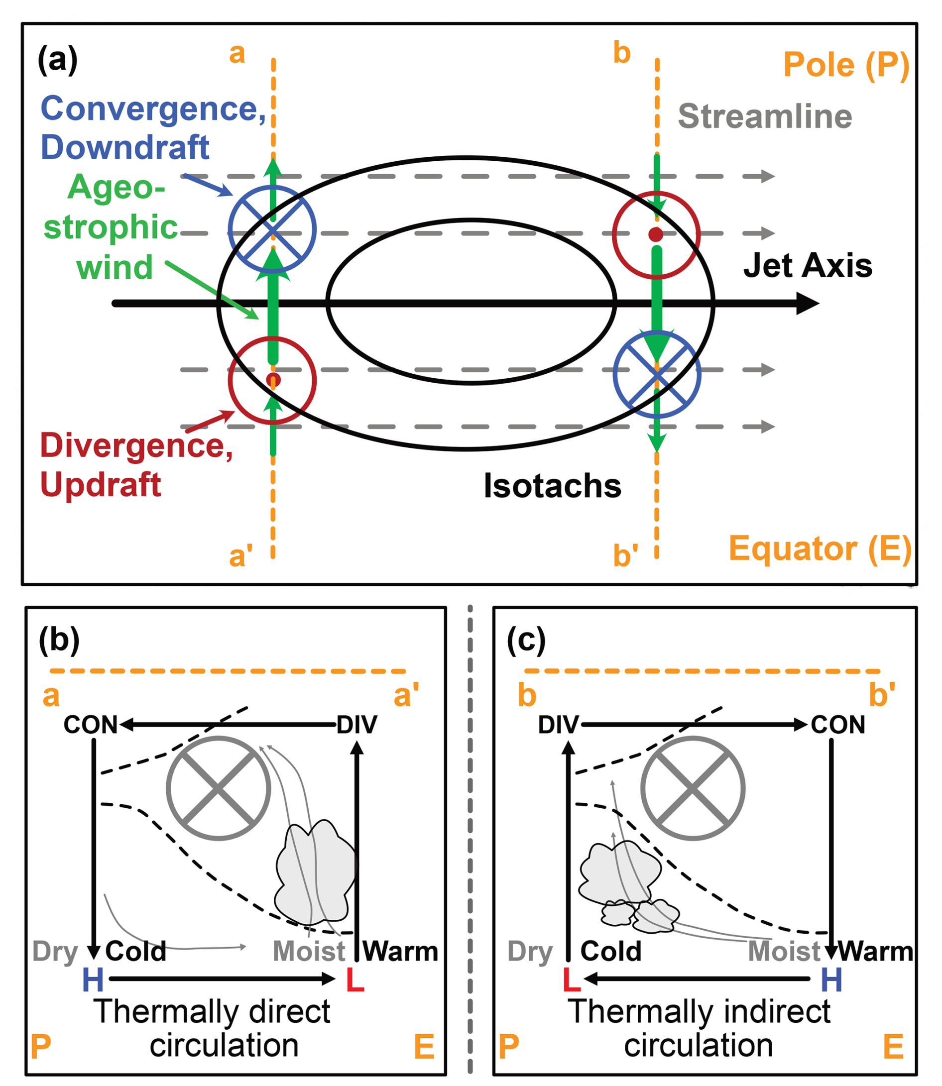
Figure 1 Schematics adapted from (a) Beebe and Bates (1955), their Fig. 4, and (b, c) Uccellini and Kocin (1987), their Fig. 3B. Panel (a) shows an idealized straight jet streak with the associated upper-level convergence and divergence and induced updraughts (dotted red circles) and downdraughts (blue circles with cross). Green arrows show the direction of ageostrophic wind for a straight jet streak (upward in the panel being poleward). Dashed orange lines show the cross-sections whose transverse circulation is depicted in panels (b) and (c). In panels (b) and (c), black arrows show ageostrophic transverse motion around the jet. Dashed black contours illustrate example isentropes. Grey areas indicate clouds, where transverse motion can induce condensation, the intensification or genesis of cyclones, and convective processes. Thin grey arrows show exemplary streamlines in such a transverse motion, and the blue H and red L indicate where transverse motion can support the formation of surface high- and low-pressure systems, respectively.

The potential vorticity (PV) perspective provides a powerful framework to study jet streaks due to (i) PV conservation under adiabatic flow (Ertel, 1942) and (ii) the invertibility property (Hoskins et al., 1985), both of which allow the study of the role of adiabatic and diabatic processes during the life cycle of jet streaks. The PV perspective (Hoskins and James, 2014) has been employed to study the dynamics of extratropical cyclones and accompanying jet streaks (see, for example, Gyakum, 1983; Boyle and Bosart, 1986; Wernli et al., 2002; Binder et al., 2016; Martínez-Alvarado et al., 2016) and specifically the influence of diabatic processes on extratropical cyclone dynamics (Hoskins et al., 1985; Hoskins and Berrisford, 1988; Davis and Emanuel, 1991; Grams et al., 2011; Schemm et al., 2013; Davies and Didone, 2013; Schemm and Wernli, 2014; Saffin et al., 2021; Attinger et al., 2021), including the formation of blocking (Pfahl et al., 2015; Steinfeld et al., 2020). Davies and Rossa (1998) established a quantitative link between isentropic wind speed and PV gradients and analysed the dynamics of jet streaks, viewed as regions of enhanced PV gradients, as PV frontogenesis under the assumption of adiabatic flow. Considering the utility of the PV gradient as a proxy for the jet, Bukenberger et al. (2023) expanded upon the work of Davies and Rossa (1998) using a 3D Lagrangian PV gradient perspective to quantify the influence of diabatic processes on jet streak evolution. A key finding of Bukenberger et al. (2023) is the prominent role of diabatic PV gradient modification in the case of strong jet streaks, which is consistent with the climatological study by Winters (2021) on extreme North Atlantic winter jet streaks. Regions of enhanced PV gradients are linked to Rossby wave guidability (Martius et al., 2010; Manola et al., 2013; Branstator and Teng, 2017; Wirth, 2020; Polster and Wirth, 2023), enabling the study of Rossby wave dynamics by means of the PV gradient perspective.

This study employs a PV gradient framework in conjunction with a jet streak identification and tracking algorithm and statistical clustering techniques to provide a comprehensive quantification of the life cycle properties of North Atlantic jet streaks. More specifically, the following research question are addressed:

1. Is there a relationship between jet streak intensity and lifetime and other characteristics such as their area, the maximum PV gradient, and isentropic level?

2. Is there an archetypal jet streak life cycle over the North Atlantic?

3. What is the large-scale flow situation as jet streaks reach their peak intensity?

4. What is the role of diabatic processes in jet streak evolution? Is it different for extreme vs. non-extreme jet streaks?

The methods to identify, track, and cluster jet streaks are presented in Sect. 2.1.2 and 2.2. In Sect. 2.6, the fundamental link between the isentropic PV gradient and horizontal wind speed is revisited. Section 3 presents the results, the core of which is a systematic composite study based on jet streaks clustered into different categories according to their large-scale dynamical environment (Sect. 3.4). Finally, we summarize our findings and provide an outlook for future research in Sect. 4.

2 Methods and data

This study uses 6-hourly ECMWF reanalysis version 5 (ERA5) data for the winter (DJF) period in the Northern Hemisphere between 1979 and 2023, interpolated to a regular 0.5° latitude–longitude grid in the horizontal dimension (Hersbach et al., 2020; Hersbach et al., 2023). In the vertical dimension, the data are interpolated onto 26 isentropic levels between 310 and 360 K in steps of 2 K. Global satellite coverage began contributing to ERA5 from 1979 onward. This addition improved reanalysis quality and made upper-level winds and extreme speeds more reliable, especially over oceans like the North Atlantic. Hence, using data from 1979 onward ensures a high-quality and consistent basis for our analysis.

To effectively use the PV gradient as a proxy for wind speed, theory requires spatial low-pass filtering for both PV and wind data (Bukenberger et al., 2023). The low-pass filtering used here involves transforming the PV and wind fields into spherical harmonics space and applying a triangular truncation at spherical harmonics of degree 80. Instead of a sharp cutoff, we use a Gaussian decay to smoothly suppress modes of a higher degree. More precisely, the spherical expansion of the field is given by

$$\begin{array}{}\text{(1)}& f(\mathit{\lambda },\mathit{\varphi })=\sum _{l=\mathrm{0}}^N\sum _{m=-l}^l{f}_l^m{Y}_l^m(\mathit{\lambda },\mathit{\varphi }),\end{array}$$

where $Y_l^m(\mathit{\lambda },\mathit{\varphi })$ is the spherical harmonic function of degree l and order m and $f_l^m$ is the corresponding coefficient. The filtered field is

$$\begin{array}{}\text{(2)}& \stackrel{\mathrm{̃}}{f}(\mathit{\lambda },\mathit{\varphi })=\sum _{l=\mathrm{0}}^N{e}^{-(l/\mathit{\sigma }{)}^{\mathrm{2}}}\sum _{m=-l}^l{f}_l^m{Y}_l^m(\mathit{\lambda },\mathit{\varphi }),\end{array}$$

with σ=80. The zonal wavenumber is m, and the meridional wavenumber is l−m; thus, for a zonal wavenumber m=0 and l=σ and the Earth's circumference of 2πr₀≈40 000 km, this yields a meridional wavelength of approximately 500 km. Hence, the filtering gives little weight to wavelengths smaller than 500 km. We refer to low-pass-filtered wind as wind and low-pass-filtered PV as PV from now on, unless stated otherwise.

2.1 Jet streak identification and tracking

To identify and track jet streaks, we use a time series of jet streak centre locations, $r_{\mathrm{js}}\left(t\right)={\left[{\mathit{\theta }}_{\mathrm{js}}\left(t\right),{\mathit{\varphi }}_{\mathrm{js}}\left(t\right),{\mathit{\lambda }}_{\mathrm{js}}\left(t\right)\right]}^T$, where the isentrope θ_js(t) is the isentrope with maximal wind speed at time t. Further, λ_js(t) in degrees east is the jet streak centre longitude, and ϕ_js(t) in degrees north is the latitude of the jet streak centre.

2.1.1 Identification

The algorithm to determine r_js(t) uses isentropic horizontal wind speed and PV. The three central steps of the algorithm, which are also illustrated in Fig. 2, are as follows:

1. Central isentrope. The isentrope that exhibits maximum wind speed is identified (Fig. 2a). The search includes isentropes between 310 and 360 K, with intervals of 2 K. The maximum wind speed is denoted jet streak intensity and the corresponding isentrope the central isentrope.

2. Central longitude. First, a percentile threshold (99.25 %) of the instantaneous wind speed on the central isentrope is used to create a coherent area of high wind speeds around the wind speed maximum that is not sensitive to its exact location. The median of the mask's longitudinal extent is defined as the central longitude (see Fig. 2b). If the wind speed maximum is positioned close to (±2.5° E) the boundary of the North Atlantic domain (defined as 20–75° N × 100° W–0° E in this study), we compute the central longitude at this distance to the domain boundary¹.

3. Central latitude. The central latitude is the latitude with the minimum distance between the dynamical tropopause (2 PVU) and the PV at the location of the central longitude (see Fig. 2c). In the present implementation, we require the central latitude to lie within ±5° N of the maximum wind along the central longitude.

Additionally, the jet streak centre is only accepted if the wind speed at its position is larger than 35 m s⁻¹. This ensures that the jet streak centre is embedded in the jet stream and that our threshold is in the range of thresholds typically used to define in-jet wind speeds, as in Hartmann (2007), Eichelberger and Hartmann (2007), and Messori et al. (2021) for zonally averaged zonal wind speeds and Winters (2021) and Simmons (2022) for typical wind speeds in the North Atlantic jet stream. The percentile threshold of 99.25 % was determined empirically, with the goal of creating a mask of very high wind speed that consists of a single connected patch containing the location of maximum wind speed for most time steps. Additionally, the mask should be large enough to ensure that the position of the jet streak centre is robust toward small-scale wind speed variations close to the maximum wind speed. The projection onto the intersection with the tropopause in the last step is done to achieve tropopause-centred composites at a later stage.

Figure 2 Schematic illustrating the jet streak centre identification algorithm. Panel (a) illustrates the identification of the central isentrope. The 2D fields on different isentropes show the 2 PVU isoline (black contours; with PVU being the unit of potential vorticity (PV), i.e. 1 PVU = 10⁻⁶ K kg⁻¹ m² s⁻¹) and the horizontal wind speed 35 m s⁻¹ isotach (blue contours). The red dots on each isentrope indicate the position of the wind speed maximum per isentrope. Scatters to the right (red dots) show the max wind on each isentrope, and the red arrow points to the central jet streak isentrope. Panel (b) shows the calculation of central longitude. Contours show the same variables as in panel (a) on the central isentrope. The blue shading masks the 99.25 percentile of instantaneous wind on the central isentrope, black lines surrounding blue shading indicate the outermost longitudes of the 99.25 percentile wind speed mask, and the black line in the middle of the blue shading indicates the central longitude of the 99.25 percentile wind mask. Panel (c) demonstrates the selection of the latitude closest to the tropopause on the central jet streak isentrope and longitude. It shows the 2 PVU isoline (dashed line) and the outermost latitudes of 35 m s⁻¹ wind speed mask on the central isentrope (vertical blue lines). Black markers show the PV at each grid point on the central isentrope and longitude (open circles), PV at each grid point on the central isentrope and longitude for which wind speed exceeds 35 m s⁻¹ (filled circles), and finally PV at the jet streak centre (red cross).

The algorithm identifies exactly one jet streak centre within the North Atlantic domain per time step. In the case of multiple jet streaks within the domain, it selects the most intense one. Hence, if a jet streak is missed, typically early in its life cycle, the algorithm accounts for it once it intensifies and eventually matures into the most intense jet streak in the North Atlantic sector. All weaker jet streaks are ignored. This implies that the mature phase of strong jet streaks is robustly captured, while results on the genesis and lysis phases must be interpreted more carefully.

2.1.2 Tracking

The zonal propagation speed of jet streaks exhibits only a weak case-by-case variability (Fig. 3). Roughly 85 % of all 6-hourly distances between two consecutive time steps are within $[-\mathrm{3},+\mathrm{12}]$° (6 h)⁻¹. Hence, two jet streak centres are linked to the same life cycle if the zonal distance between both can be covered by a zonal velocity from the above velocity range and within a time period of 24 h. A jet streak life cycle must have a minimum duration of 18 h (three steps) and gaps of up to 24 h (four steps) are allowed, whereby each fragment of the life cycle must be at least 6 h (one step) long.

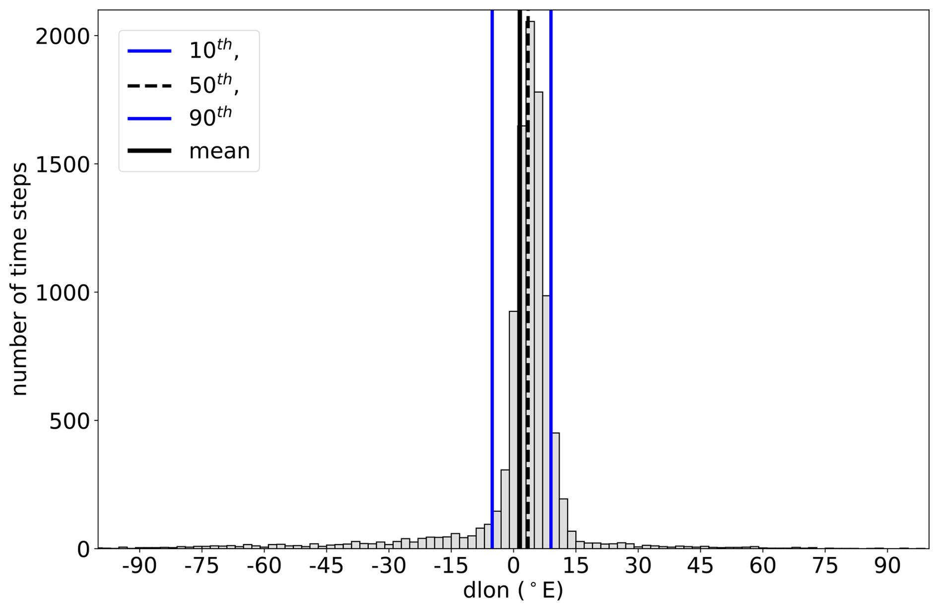
Figure 3 Histogram of 6-hourly differences in longitudinal position of jet streak centres, calculated with the method detailed in Sect. 2.1.1. The vertical lines show the mean (solid black), median (dashed black), and the 10th and 90th percentiles (blue) of 6-hourly differences in longitudinal position of jet streak centres.

2.1.3 Life cycle characteristic

After calculating jet streak centres for each time step and assigning event labels, the characteristic properties of jet streak life cycles can be analysed. To this end, the following definitions are used:

1. The first time step assigned to a jet streak event is called genesis.

2. The last time step assigned to a jet streak event is called lysis.

3. The maximum jet streak intensity (i.e. maximum wind speed) during a jet streak event is defined as its peak intensity. The corresponding isentrope is used to compute the intensification rate throughout the life cycle.

4. The time between genesis and peak intensity is called the intensification phase.

The identification of peak intensity and intensification is illustrated in Fig. 4c. The jet streak intensification rate is defined as the 6-hourly difference between the wind speed maxima in a jet streak object. It should be noted that the intensification rate is calculated on a fixed isentropic level, i.e. the isentropic level exhibiting the maximum wind speed throughout the entire life cycle and therefore denoting the acceleration of the wind on the level at which the maximum wind speed throughout the life cycle occurs. The maximum rate is denoted the peak intensification rate.

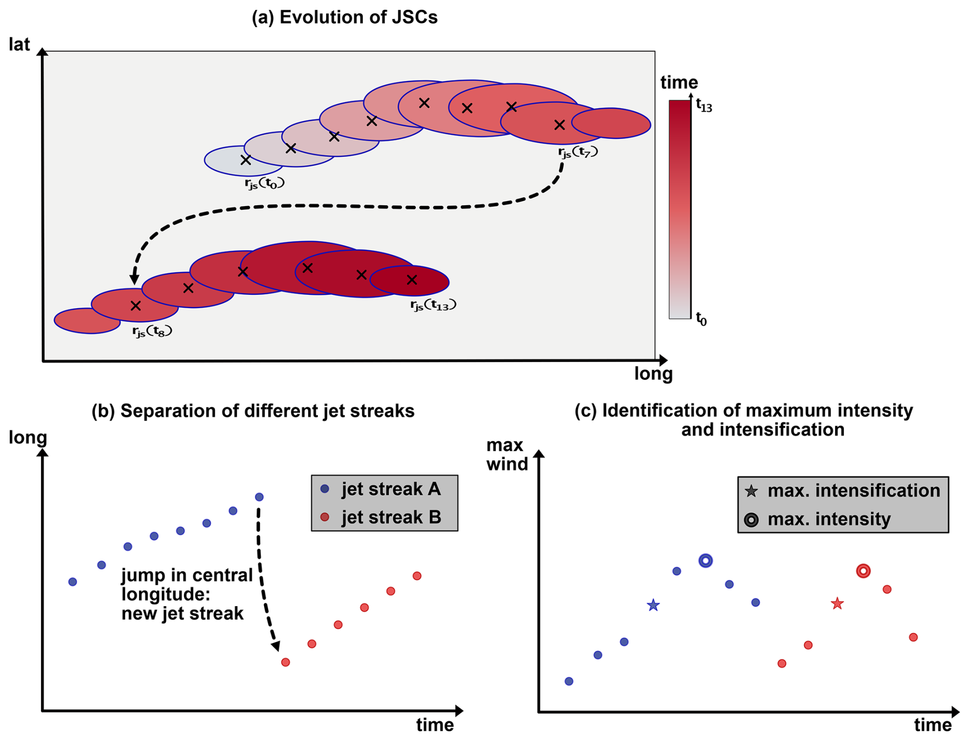
Figure 4 Schematic illustrating the algorithms (a, b) tracking jet streak events and (c) identifying their times of peak intensification and intensity. Panel (a) shows the wind speed on central isentropes for 14 consecutive time steps at 35 m⁻¹ (blue contours), the jet streak centres (black crosses), and the time step (colours from white to red). The dashed arrow indicates the longitudinal jump in the jet streak centre between the end of first and the beginning of second jet streak. Panel (b) shows jet streak centre longitude against time and jet streak centres of the first (blue dots) and second (red dots) jet streak. Panel (c) shows the wind speed maximum on the central isentrope against time for the wind speed maximum of the first (blue markers) and second (red markers) jet streak. Stars and open circles indicate the time steps of peak jet streak intensification and intensity, respectively.

The streak tracking algorithm allows the identification of the evolution of the central isentrope throughout jet streak evolution and shows that for 80 % of jet streaks, the central isentrope at the time of peak jet streak intensification is within a 5 K distance relative to the isentrope at peak intensity (Fig. A1). While for our analysis, using the central isentrope at the time of peak jet streak intensity is useful to show the dynamical evolution on this level (Sect. 3.4), following the instantaneous isentropic level throughout the jet streak evolution might be more appropriate for other research questions.

2.2 Clustering of jet streak events

2.2.1 Jet stream regimes

To connect jet streak life cycle characteristics with the state of the eddy-driven jet stream, we use a jet stream regime definition similar to that introduced by Frame et al. (2011). The regime definition relies on zonally averaged but meridionally varying jet profiles, denoted U(t,ϕ), which are computed by zonally and vertically averaging the zonal wind between 60 and 0° W and between 700 and 900 hPa. The North Atlantic winter jet stream is known to have three preferred meridional positions (Woollings et al., 2010, their Fig. 1). Since this discovery, the three jet regimes and transitions between them have been discussed in terms of an oscillator model of the North Atlantic jet stream (Frame et al., 2011; Ambaum and Novak, 2014), adding physical meaning to the statistical prevalence of these positions. Therefore, we apply K-means clustering (Jain, 2010) with 3 degrees of freedom to the jet profiles U(t,ϕ). K means is an unsupervised clustering method that separates input data into K clusters by minimizing within-cluster variance and maximizing between-cluster variance. The three clusters, which are denoted S (southern), M (middle), and N (northern), correspond to different states of the North Atlantic jet stream (Frame et al., 2011). Each time step can now be associated with one of the three regimes. Jet streaks that reach their peak intensity at a time associated with an S, M, or N regime are called S-, M-, or N-regime jet streaks, respectively.

2.2.2 Clustering upper-level flow regimes

To classify synoptic situations where jet streaks intensify, we use a self-organizing map (SOM; Kohonen, 1995) combined with agglomerative clustering. SOM is well established in the study of synoptic-scale circulation features (see, e.g. Liu and Weisberg, 2011) and organizes data into a 2D grid of $k=m\times n$ nodes, each representing one of k reference vectors.

SOM clustering places similar nodes closer together and dissimilar nodes farther apart on its m×n grid, using a distance metric and a neighbourhood function to calculate the references vectors represented by each node (Hewitson and Crane, 2002). We refer the reader to Appendix E for a detailed description of the SOM clustering method. SOM, while not strictly minimizing within-cluster variance or maximizing between-cluster variance, as is the case for K-means clustering, provides a highly interpretable 2D map (Kohonen, 2013). The map thereby illustrates high-density regions in the input data space, allowing us to estimate an appropriate number of clusters without prior knowledge. SOM clustering therefore requires less knowledge about the ideal number of clusters in advance, which is why we chose it as a complementary approach.

We apply SOM clustering to isentropic PV fields at peak intensification and intensity on the central jet streak isentrope for all jet streaks. After remapping a jet streak's centre to (0.0° N, 0.0° E) with an area-preserving coordinate transformation (Sect. 2.3), PV fields are restricted to a box from 50° E to 50° W and from 25° N to 30° S and normalized to [0,1] using minimum–maximum scaling before SOM clustering is performed. The map's size determines the balance between accurately representing synoptic features (more nodes) and a substantial reduction in dimensionality (fewer nodes) with respect to the input data space. After manually testing several SOM shapes and evaluating standard metrics like quantization and topographic error (see Kohonen, 1995; Kiviluoto, 1996, for the definition and usage of those quantities), we chose a 7 × 5 map as the basis of our agglomerative clustering (see Appendix E for details).

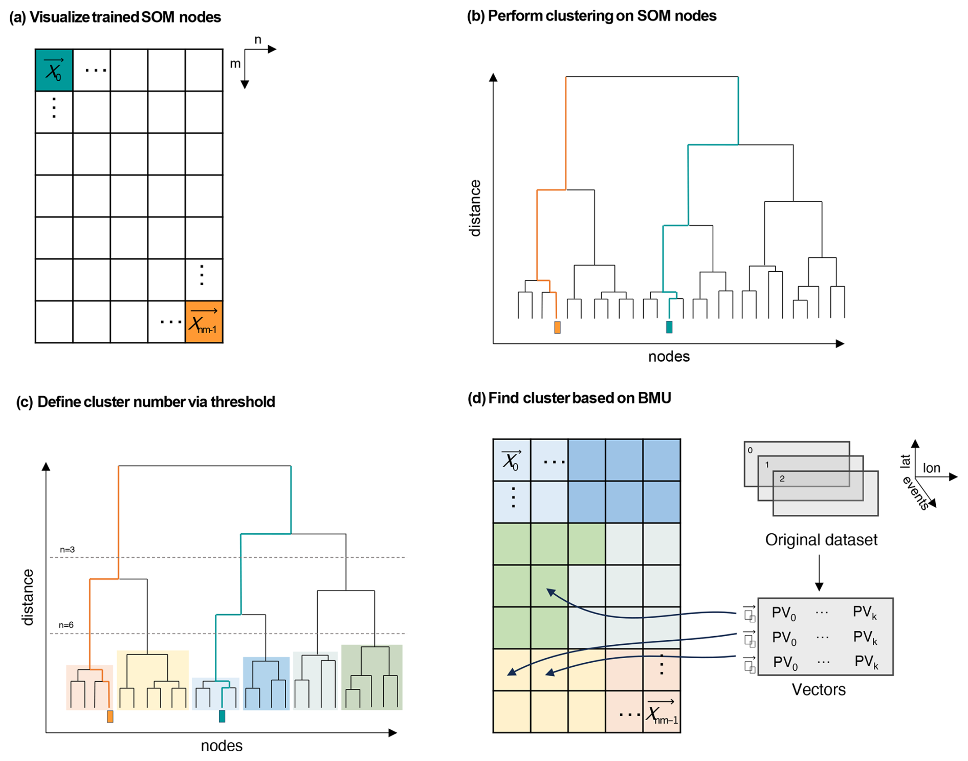
Figure 5 Visualization of the clustering process. Panel (a) shows the 2D SOM map generated through the algorithm's training with PV vectors from two different time steps, placing dissimilar nodes, which represent PV vectors, far away from each other. Panel (b) is the dendrogram, a visualization of the merging pattern of hierarchical agglomerative clustering of SOM nodes that groups those nodes. Panel (c) shows how altering thresholds of co-phenetic distance produces various cluster numbers. Panel (d) assigns each original PV vector to a reference vector of the SOM and thus to a cluster. Within each vector, PV₀ is the normalized PV value at the first grid point for the time of peak jet streak intensification, and PV_k is the normalized PV value on the last grid point at the time of peak jet streak intensity.

This step (Fig. 5b) further reduces the number of clusters by the use of a dendrogram of SOM nodes based on normalized PV maps. The dendrogram's y axis shows the increase in within-cluster variance with each merge, indicating cluster similarity. We use a distance threshold to control maximum within-cluster variance (Gentleman, 2023), where lower thresholds produce more, smaller clusters, and higher thresholds yield fewer, larger, and more heterogeneous clusters. The threshold balances two aims: keeping distinct synoptic patterns separate and isolating clusters with high rates of extreme jet streak events. After testing, we selected six clusters to capture the evolution of synoptic features between peak intensification and intensity. Each jet streak event is assigned to a cluster based on its best-matching SOM unit, and the composite analyses based on jet-streak-centred fields for each cluster appear in Sect. 3.

2.3 Jet-streak-centred composites

To obtain the jet-streak-centred composite, the input coordinate system is rotated to position the jet streak centre at the centre for each event and time step of interest using the Climate Data Operator's (CDO's; Schulzweida, 2023) area-preserving remapping function for regular grids (Schulzweida, 2023). A composite analysis using jet-streak-centre-centred fields for non-extreme and extreme jet streaks is employed to investigate the large-scale circulation patterns in which jet streaks evolve (Sect. 3).

2.4 Bootstrap analysis

A key part of this work is the comparison of non-extreme and extreme jet streaks. Since extreme events are a small subset, bootstrapping helps test the significance of their characteristics. Bootstrapping (introduced in Efron, 1979) is frequently used to infer the probability distribution of a statistical measure of a dataset if a small but representative sample is at hand, and it is particularly useful for minimizing the impact of outliers. For some applications of bootstrapping in atmospheric and climate science, see Mason and Mimmack (1992) and Downton and Katz (1993). This method assumes that each sample member is equally likely and that therefore the sample is just one plausible realization of drawing the number of members that are part of it. Resampling with replacement then allows the approximation of the probability distribution of, for example, the mean, median, or variance of the underlying dataset.

This study uses bootstrapping to determine whether differences between extreme and non-extreme jet streaks are robust. We generate 1000 resamples of the extreme jet streaks, with each sample containing the same number of events as the original extreme set, and repeat this for non-extreme jet streaks. We use those resamples to estimate the distributions of basic jet streak characteristics and the frequency of Frame jet regimes for extreme and non-extreme jet streaks (Sect. 3.1). To determine robust differences in the flow associated with extreme vs. non-extreme jet streaks, we calculate the mean and standard deviation of composite means based on the resamples. We mark the difference between extreme and non-extreme jet streaks as robust if it exceeds the combined standard deviation of both sets (Sect. 3).

2.5 Normalized jet streak occurrence

To analyse the evolution and occurrence frequency of jet streaks, we compute a normalized jet streak centre probability density function (PDF). It represents the likelihood of a jet streak centre occurring over a given region. The normalized PDF is obtained by fitting a Gaussian PDF to selected jet streak centres on the regular ERA5 grid, giving equal weight to each event. Afterwards, the Gaussian-smoothed field is divided by the total number of identified jet streaks. Finally, the field is weighted by the inverse area of each grid point. The integral of this field over the Earth's surface evaluates to 1. This method ensures comparability of the normalized PDF between selected subsets of all jet streaks (e.g. non-extreme vs. extreme event climatologies).

2.6 A PV gradient perspective on jet streaks

PV on an isentropic surface is defined as

$$\begin{array}{}\text{(3)}& \mathrm{PV}={\displaystyle \frac{\mathit{\zeta }+f}{\mathit{\sigma }}},\end{array}$$

where ζ is the isentropic relative vorticity, f=2Ωsin (ϕ) represents the Coriolis parameter, and the isentropic density $\mathit{\sigma }=-(\mathrm{1}/g){\partial }_{\mathit{\theta }}p$ is a measure of stratification. PV is given in units of 1 PVU = 10⁻⁶ K m² kg⁻¹ s⁻¹ throughout this work. As shown in Martius et al. (2010) and Bukenberger et al. (2023), the isentropic PV gradient ($\Vert {\mathrm{\nabla }}_{\mathit{\theta }}\mathrm{PV}\Vert$) can be considered a proxy for the horizontal Laplacian of wind speed under certain flow conditions, i.e.

$$\begin{array}{}\text{(4)}& \Vert {\mathrm{\nabla }}_{\mathit{\theta }}\mathrm{PV}\Vert \approx -{\displaystyle \frac{\mathrm{1}}{{\mathit{\sigma }}_{\mathrm{0}}}}△U,\end{array}$$

​​​​​​​where σ₀ is the isentropic density of the background flow, and U is the horizontal wind speed. If variations in wind speed are dominated by a mode of wavelength λ, a direct proportionality between wind speed and the PV gradient emerges:

$$\begin{array}{}\text{(5)}& \Vert {\mathrm{\nabla }}_{\mathit{\theta }}\mathrm{PV}\Vert \approx {\displaystyle \frac{\mathrm{4}{\mathit{\pi }}^{\mathrm{2}}}{{\mathit{\lambda }}^{\mathrm{2}}{\mathit{\sigma }}_{\mathrm{0}}}}U.\end{array}$$

In flow situations where Eq. (4) is a good approximation, the PV gradient serves as an analytical tool to connect jet streak evolution to diabatic processes. For wind speeds representing a superposition of multiple modes, shorter wavelengths dominate the PV gradient, which is therefore best used after applying a low-pass filter to the PV and wind fields. The following paragraph presents the analytical approach and assumptions underlying the quantitative link between the PV gradient and variations in horizontal relative vorticity, insofar as they are important for the understanding of this study. Bukenberger et al. (2023) presents a detailed version of the analysis. The basic idea is to consider a perturbation to a background flow characterized by constant wind, the Coriolis parameter, and stratification.

Developing the Taylor polynomial of the PV gradient up to the second order in perturbations that we assume are much smaller than the background flow and under the condition that variations in the perturbation of stratification are much smaller than the horizontal Laplacian of wind speed; i.e. for slowly varying stability and in the case of the large △U common in jet streaks, the PV gradient is approximated well by

$$\begin{array}{}\text{(6)}& \Vert {\mathrm{\nabla }}_{\mathit{\theta }}\mathrm{PV}\Vert \approx -{\displaystyle \frac{\mathrm{1}-\frac{{\mathit{\sigma }}^{\prime }}{{\mathit{\sigma }}_{\mathrm{0}}}}{{\mathit{\sigma }}_{\mathrm{0}}}}△U.\end{array}$$

Following an identical approach to the gradient of the logarithm of PV, $\Vert {\mathrm{\nabla }}_{\mathit{\theta }}\ln \left(\mathrm{PV}\right)\Vert$, which is also a good proxy for Rossby wave guidability (Polster and Wirth, 2023), yields – under the same conditions –

$$\begin{array}{}\text{(7)}& \Vert {\mathrm{\nabla }}_{\mathit{\theta }}\ln \left(\mathrm{PV}\right)\Vert \approx -{\displaystyle \frac{\mathrm{1}-\frac{f^{\prime }+{\mathit{\zeta }}^{\prime }}{f_{\mathrm{0}}}}{f_{\mathrm{0}}}}△U.\end{array}$$

If perturbations in stability are much smaller than the background stability, Eq. (6) simplifies to Eq. (4). In the case of small vorticity perturbations, Eq. (7) becomes

$$\begin{array}{}\text{(8)}& \Vert {\mathrm{\nabla }}_{\mathit{\theta }}\ln \left(\mathrm{PV}\right)\Vert \approx -{\displaystyle \frac{\mathrm{1}}{f_{\mathrm{0}}}}△U.\end{array}$$

Observations reveal a systematic stratospheric displacement of bands with a high PV gradient compared to regions of maximum wind speed. This displacement is elucidated by the sharp increase in stability when transitioning from the tropospheric to the stratospheric side of the jet, leading to an increase in $\mathrm{1}-\frac{{\mathit{\sigma }}^{\prime }}{{\mathit{\sigma }}_{\mathrm{0}}}$. The relationship between $\Vert {\mathrm{\nabla }}_{\mathit{\theta }}\ln \left(\mathrm{PV}\right)\Vert$ and △U is less sensitive to perturbations in stability near the tropopause. If variations in the relative vorticity are not too large, bands of high $\Vert {\mathrm{\nabla }}_{\mathit{\theta }}\ln \left(\mathrm{PV}\right)\Vert$ are aligned well with jet maxima. This makes $\Vert {\mathrm{\nabla }}_{\mathit{\theta }}\ln \left(\mathrm{PV}\right)\Vert$ a superior diagnostic for jet strength and wave guidability as long as the jet is not excessively strong or narrow. For extreme jet streaks, often associated with bands of negative PV on the tropospheric side of the jet, the PV gradient becomes the superior diagnostic.

In flow situations in which Eq. (4) is a good approximation, corresponding to balanced flow situations, the PV gradient serves as a proxy variable to connect jet streak evolution to diabatic processes. Although PV is materially conserved in adiabatic flow situations, the PV gradient can be modified by deformation and shear. A Lagrangian perspective on PV gradient evolution, disentangling diabatic and adiabatic contributions to changes in $\Vert {\mathrm{\nabla }}_{\mathit{\theta }}\left(\mathrm{PV}\right)\Vert$, as demonstrated in Bukenberger et al. (2023), offers a unique opportunity to quantify the influence of diabatic processes on upper-level jet dynamics.

Even if a direct link between PV gradients and wind speeds cannot be established, regions of a high PV gradient still indicate significant variations in both wind and thermal stratification on tropopause-intersecting isentropic surfaces. This is particularly likely in flow situations far from geostrophic balance, such as those occurring in regions of enhanced diabatic activity or during strong jet streak intensification. In these situations, the PV gradient perspective remains meaningful for studying jet streak dynamics, especially when considering jet streaks in close connection to upper-level frontogenesis and changes in stratification.

Figure 6 illustrates the relationship between jet streak intensity and the PV gradient at the jet streak centre at the time of peak jet streak intensity. A linear fit describes this relationship. The correlation between maximum wind speed and PV gradient at the jet streak centre at the time of peak jet streak intensity is 0.28. Due to the considerable variability in jet streak width and tropopause stability, the observed limited correlation and imperfect fit are expected. Despite these complicating factors, the PV gradient proves to be a reliable indicator of jet streak intensity. This analysis underscores the utility of the PV gradient framework for investigating jet streak dynamics.

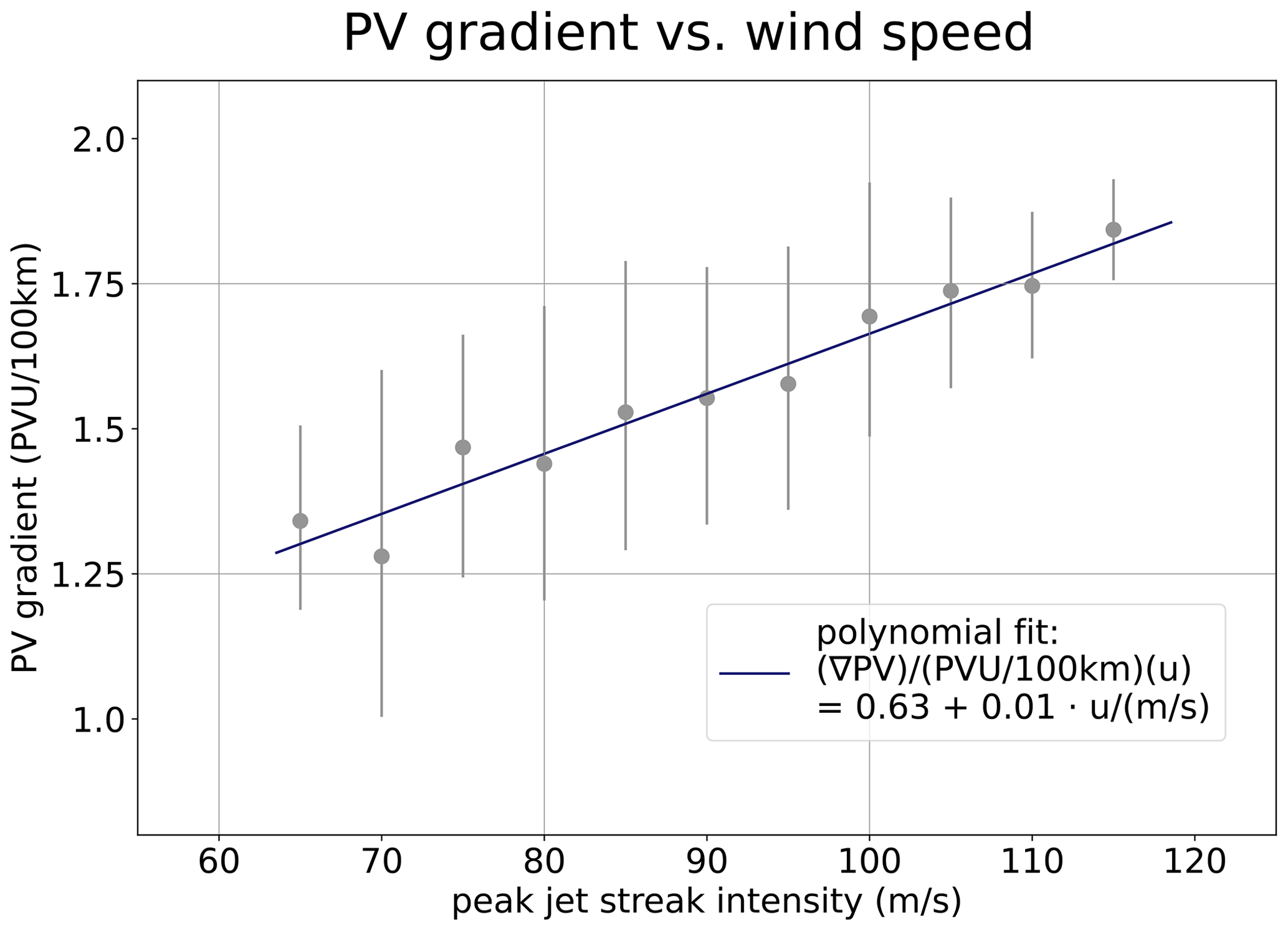
Figure 6 Relationship between the PV gradient at the jet streak centre and the maximum wind speed at the time of peak jet streak intensity. The solid blue line shows a Gaussian fit to a polynomial of the first degree of the norm of the PV gradient at the jet streak centre, depending on the maximum wind speed based on the times of peak jet streak intensity for all 1050 jet streaks. The correlation between maximum wind speed and norm of the PV gradient at the jet streak centre for this time is 0.28. The position of each grey marker on the y axis indicates the mean norm of the PV gradient at the jet streak centre for jet streaks with a maximum wind speed within 2.5 m s⁻¹ of its position on the x axis. Each vertical grey bar spans the 20th–80th percentile of the PV gradient at the jet streak centre for jet streaks with a maximum wind speed within 2.5 m s⁻¹ of their positions on the x axis.

3 Results

3.1 Characteristics of North Atlantic winter jet streaks

We begin with an examination of basic jet streak life cycle characteristics. The distribution of peak intensity of all 1050 jet streaks exhibits a nearly symmetric shape, with a standard deviation of 8.6 m s⁻¹ around a mean value of 87.3 m s⁻¹ (solid black line and grey box in Fig. 7a). Closer inspection reveals a mild skew towards higher peak intensities. The median peak jet streak intensity is 86.8 m s⁻¹, while the 5th and 95th percentiles are 73.5 and 101.9 m s⁻¹, respectively. For a robust definition of extreme jet streaks, we chose extreme events combining high wind speed and large areas, also avoiding detection of single grid points exceeding a wind threshold. We define the wind speed threshold based on the wind speed distribution over the North Atlantic. A wind speed exceeding the 99.9th percentile for at least 90 % of North Atlantic grid points on all isentropes is 92.5 m s⁻¹, which we therefore set as the wind speed threshold. Figure 7b shows the distribution of the area covered by wind speeds exceeding 92.5 m s⁻¹ at the time of peak intensity on the central isentrope for the 310 jet streaks for which peak intensities exceed this threshold. The 50th percentile of the area with wind speed exceeding 92.5 m s⁻¹ for those jet streaks is 1.91×10⁵ km², while the 70th and 90th percentiles are 3.62×10⁵ and 6.46×10⁵ km², respectively. We define extreme jet streaks as events for which the area on which wind speeds exceed 92.5 m s⁻¹ is larger than 3.62×10⁵ km² at the time of their peak intensity, a definition yielding 91 extreme events.

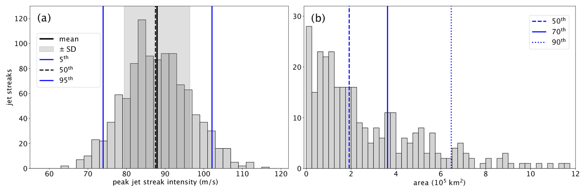
Figure 7 Jet streak characteristics at the time of peak intensity. (a) Histogram of peak intensity for all 1050 jet streaks with a bin width of 2 m s⁻¹. The light-grey area indicates the width of the standard deviation around the mean wind speed, and vertical lines are the mean (solid black), median (dashed black), and 5th and 95th percentiles (thin solid blue) of the distribution. (b) Histogram of area with wind speed exceeding 92.5 m s⁻¹ at peak jet streak intensities exceeding 92.5 m s⁻¹, with a bin width of 0.25×10⁵ km² and vertical blue lines indicating the 50th (dashed), 70th (solid), and 90th (dotted) percentiles.

3.1.1 Relationship with jet regimes

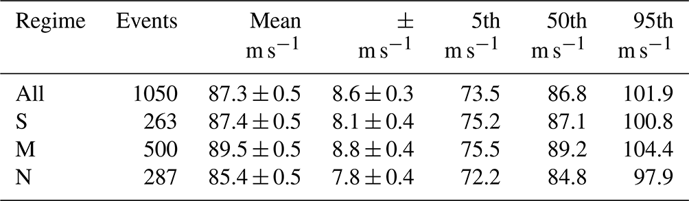
We find some variations in jet streak characteristics in the three large-scale jet regimes of Frame et al. (2011). The M-regime jet streak distribution, comprising 500 jet streak maxima, exhibits slightly but robustly higher peak intensities compared to the total climatology. The N regime, involving 287 jet streaks, features weaker jet streaks and smaller variability, and the distribution of S-regime jet streak maxima closely mirrors the overall climatology (Table 1). While those distinct mean peak jet streak intensities in different Frame regimes are consistently reproduced in a bootstrap analysis (not shown), they are well within 1 standard deviation of each other. The results of the stronger upper-level jet streak intensity for M-regime jets align with the findings of Frame et al. (2011) and Woollings et al. (2010), who showed that M-regime jets skew towards higher wind speeds compared to those in the S and N regimes.

Table 1 Characteristic properties of the distribution of peak jet streak intensity for all jet streaks and for jet streaks reaching their peak intensity in an S, M, or N regime. Shown are the mean; the standard deviation (±); and the 5th, 50th, and 95th percentiles of peak jet streak intensity based on the 1000 bootstrapping resamples described in Sect. 2. The standard deviation of the mean and the standard deviation based on 1000 bootstrapping resamples are also given.

3.1.2 Variability and trends (1979–2023)

Figure 8 shows the evolution of the winter mean and maximum peak jet streak intensities over DJF from 1979 to 2023 in ERA5. The winter-mean peak jet streak intensity (dark red and blue bars) shows an increase at a rate of 0.057 m s⁻¹ yr⁻¹, starting at 86.6 m s⁻¹ in 1979. The winter-maximum peak jet streak intensity shows at trend of 0.12 m s⁻¹, starting at 102.0 m s⁻¹ in 1979. Notably, 7 of the 10 strongest extreme jet streak events occurred after 2005. The number of extreme events per winter also shows an upward trend over the ERA5 period, although interannual and interdecadal variability are larger than the trend.

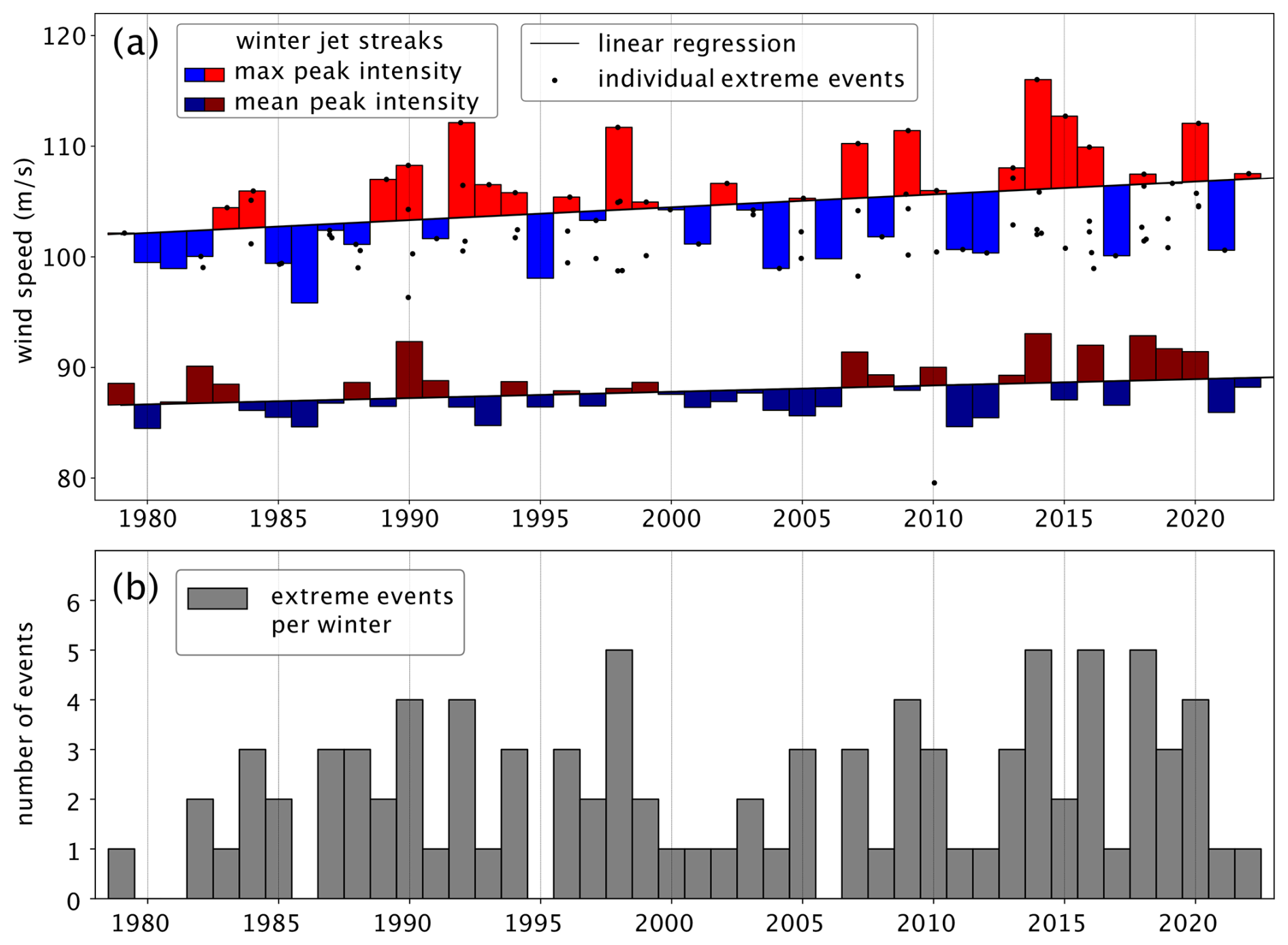
Figure 8 Temporal evolution of North Atlantic winter (extreme) jet streaks. (a) Mean and maximum peak North Atlantic winter jet streak intensity. Black dots are the individual extreme jet streak events. Dark red and dark blue bars indicate winter means of peak jet streak intensities (m s⁻¹), with red or blue bars plotted according to whether they are above or below the least-squares fit linear regression for the period of 1979–2023. Light red and blue bars indicate winter maxima of peak jet streak intensities (m s⁻¹), i.e. the peak intensity of the strongest jet streak event of each year. (b) Extreme events per winter across the ERA5 time span. Grey bars show the number of extreme jet streak events per winter.

Both the winter-mean and winter-maximum peak jet streak intensities show smaller trends than the interdecadal variability. These results are well in line with Simmons (2022), who also found a slight upward trend in monthly maximum wind speed (0.067 ± 0.048 m s⁻¹ yr⁻¹) over North America and the Atlantic (see their Fig. 16a). To evaluate the statistical significance and methodological sensitivity of those trends, it would be beneficial to compare different reanalysis datasets (e.g. the Japanese 55-year Reanalysis (JRA-55; Kobayashi et al., 2015) and NASA's Modern-Era Retrospective analysis for Research and Applications, Version 2 (MERRA-2; Gelaro et al., 2017)) and also include a dataset using a fixed observational basis, for example the NOAA–CIRES 20th Century Reanalysis (NCEP-20C; Compo et al., 2011). The trend in the maximum peak jet streak intensity is almost twice as large as the trend in mean peak jet streak intensity. This is consistent with the findings of Hermoso and Schemm (2024) and future scenario studies by Shaw and Miyawaki (2023), who observed that extreme wind speeds are increasing at a faster rate than average wind speeds. Although this trend has not yet reached statistical significance, it is expected to do so by 2050. We also observe a correlation of 0.56 between the mean and maximum peak jet streak intensity. In winters with a mean jet streak intensity above the linear trend, the maximum jet streak intensity tends to show positive anomalies and vice versa in winters with a mean below the trend.

3.1.3 Central isentropes at peak jet streak intensity

The distribution of θ_peak of all jet streaks (grey bars in Fig. 9) shows a first peak at 328 K and is skewed toward higher isentropes, with several events peaking at or above 340 K. Jet streaks with high central isentropes peak more southerly and at lower intensities than the average jet streak, suggesting that the maximum at high isentropes represents shallow subtropical jet streaks (not shown). While the set of all jet streaks has central isentropes down to 310 K, the minimum central isentrope for extreme jet streaks (red in Fig. 9) is 322 K. Overall, the distribution of the central isentropes shows a smaller range that does not exceed 342 K for extreme jet streaks, suggesting that purely subtropical jet streaks rarely turn extreme. The bulk of extreme jet streaks centred around 330 K suggests that some of them are associated with superpositions of the polar and subtropical jet, a result in line with previous research on merged jet regimes (Harnik et al., 2014b; Winters et al., 2020).

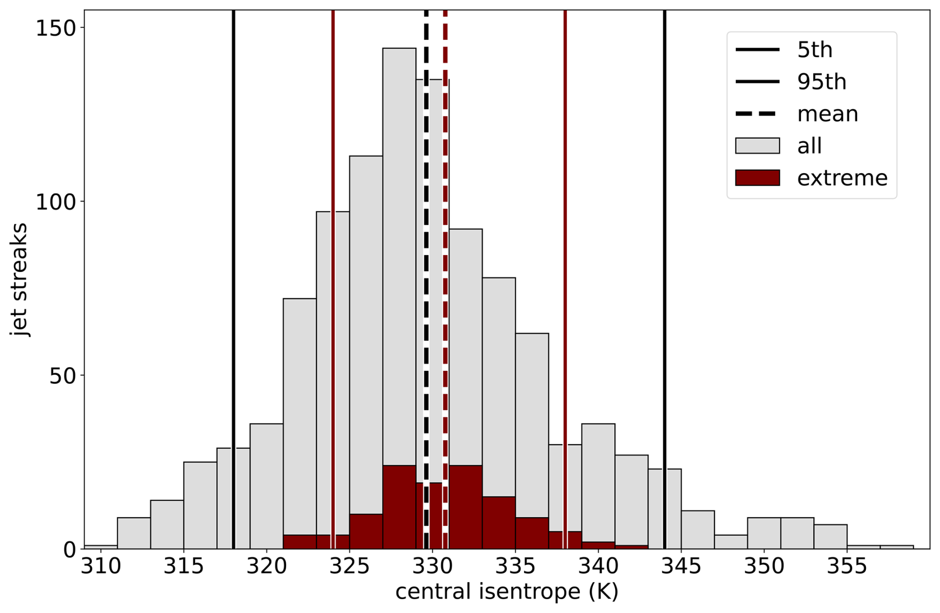
Figure 9 Histogram of central isentropes at peak jet streak intensity (θ_peak; K) for all jet streaks (grey) and for extreme jet streaks (dark red), i.e. cases with wind speeds on the central isentrope exceeding 92.5 m s⁻¹ over an area of at least 3.62 × 10⁵ km² at the time of peak jet streak intensity. Vertical lines indicate the mean (dashed) and the 5th and 95th percentiles (solid) of the distributions.

3.1.4 Jet streak lifetime and intensification phase

We proceed with the duration of different stages in jet streak evolution, examining climatologies of all and of extreme jet streaks. For all 1050 jet streaks, the median and mean jet streak lifetimes are 48 and 56 h, respectively. The 5th percentile (18 h) and 95th percentile (120 h) together indicate substantial variability and a skew toward longer lifetimes. Stratifying the dataset based on jet streak intensity, Fig. 10a presents the distributions of lifetimes for subsets of all jet streaks selected based on the peak intensity and shows that the median and mean lifetimes consistently increase with increasing peak intensity, as does lifetime variability. The median lifetime is 24 h for jet streaks with peak intensity between 60 and 68 m s⁻¹ and reaches up to 78 h for jet streaks with peak intensity between 108 and 116 m s⁻¹. Mean lifetimes are 12 h longer than medians for both groups. Despite a discernible trend toward longer lifetimes for more intense jet streaks, the median and mean lifetimes remain within the interquartile range of all jet streaks (30 to 72 h) for all but the weakest (peak intensities below 68 m s⁻¹) and strongest (peak intensities exceeding 108 m s⁻¹) events. The distribution of lifetimes for all jet streaks (Fig. 10b) provides additional context for the correlation between jet streak lifetimes and peak intensities. It illustrates an exponential decrease in occurrence as lifetimes increase. The jet streak lifetime distributions for M-, N-, and S-regime jet streaks (not shown) are all qualitatively similar to that based on the set of all jet streaks, suggesting that the lifetime of jet streaks does not exhibit a strong dependency on the jet regimes of Frame et al. (2011). Stronger jet streaks are long-lived, independent of the jet regime. However, while stratifying jet streaks by intensity reduces the variability in lifetimes somewhat for weak jet streaks, very intense jet streaks show particularly large variability. This hints at a substantial variability in the dynamics driving jet streak development, especially for strong jet streaks.

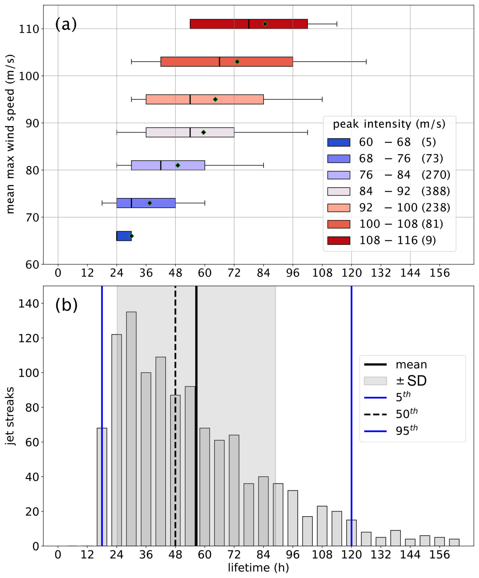
Figure 10 Analysis of jet streak lifetime. (a) Box plots for lifetime stratified by peak jet streak intensity for jet streaks with increasing peak intensities (dark blue to dark red). The position on the y axis indicates the mean peak intensity for all jet streaks in the respective category. In the box plots, the left boundary of the box indicates the 25th percentile, the vertical black line within the box the 50th percentile, and the right boundary the 75th percentile. Whiskers to the left and right indicate the 5th and 95th percentiles. The black square inside the box marks the mean of the distribution. (b) Histogram of jet streak lifetime for all jet streaks, with bins every 6 h (dark grey bars), with the light-grey area representing the width of the standard deviation around the mean lifetime, and vertical lines indicating the mean (solid black), 5th and 95th (blue), and 50th (dashed black) percentiles of the lifetime distribution.

The average jet streak intensity at genesis is 76.6 ± 7.3 m s⁻¹. The average time between genesis and peak intensification amounts to 18 h (with a median of 12 h), and it takes on average 33 h (median 24 h) for jet streaks to reach their peak intensity (87.3 ± 8.6 m s⁻¹). Jet streaks last on average 57 h (median 48 h) and exhibit a mean intensity of 79.1 ± 7.9 m s⁻¹ at their lysis, very close to the mean intensity at genesis. Note that in the mean, the intensification phase lasts about as long as the time between peak jet streak intensity and lysis. As for lifetime (Fig. 10b), the duration of jet streak intensification and the time between peak jet streak intensity and lysis are heavily skewed toward longer time spans. The mean intensification phase lasts about 1.2 times as long for extreme compared to non-extreme jet streaks, and the lifetime of extreme jet streaks is on average 1.3 times as long. For extreme jet streaks, the mean intensity at genesis is 85±7.7 m s⁻¹, 102.8±3.5 m s⁻¹ at peak intensity, and 85.6±7.8 m s⁻¹ at lysis. The acceleration rates are 0.41±0.3 (m s⁻¹) h⁻¹ for all and are slightly higher, i.e. 0.62±0.41 (m s⁻¹) h⁻¹, for extreme jet streaks. The same holds true for the decay rate between peak jet streak intensity and lysis, with $-\mathrm{0.4}\pm \mathrm{0.43}$ (m s⁻¹) h⁻¹ for all and $-\mathrm{0.65}\pm \mathrm{0.43}$ (m s⁻¹) h⁻¹ for extreme jet streaks.

To summarize, the intensification rate alone does not determine whether a jet streak evolves into an extreme. Rather, the combination of prolonged and stronger intensification is crucial. However, this result must be interpreted with caution, taking into account the large variability in intensification rates and durations. It raises the question of what sustains the intense acceleration of extreme jet streaks.

3.2 North Atlantic jet streak climatology

Examining the mean PV gradient and occurrence of wind speeds exceeding 92.5 m s⁻¹ based on low-pass-filtered wind over the North Atlantic domain (Fig. 11), we find 1405 time steps with such wind speeds over the North Atlantic in the winters of 1979–2023 in the 6-hourly ERA5 data (Fig. 11a). Such high wind speeds occur over the eastern USA, the Gulf Stream, and Canada and from the Labrador Sea northeastward past Greenland and then downstream towards the UK. The highest frequencies form a southwest–northeast-oriented band centred over the western North Atlantic and extending into the central North Atlantic. This is in qualitative agreement with the regions in which Winters (2021) found large frequencies of wind speeds exceeding 92.5 m s⁻¹.

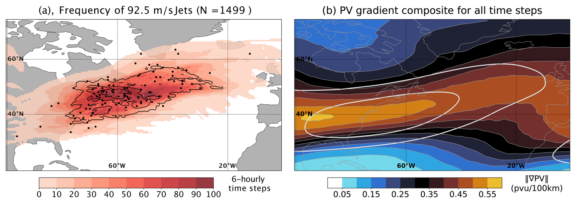
Figure 11 North Atlantic winter (DJF 1979–2020) climatologies based on 6-hourly ERA5 data. (a) Total number of 6-hourly time steps with wind speeds exceeding 92.5 m s⁻¹ on at least one isentrope over the North Atlantic domain (red colours; 20–75° N × 100° W–0° E). Contours show the number of peak jet streak intensity time steps for extreme jet streak events with wind speeds exceeding 92.5 m s⁻¹ on at least one isentrope, with contours every five time steps. Black dots show jet streak centres of extreme jet streak events at the time of peak intensity. (b) PV gradient climatology (in colours), using 6-hourly ERA5 data at 330 K (the mean of all central isentropes at the time of peak jet streak intensity). The contours are as follows: thin grey – climatology of the PV gradient with contours every 0.05 PVU (100 km)⁻¹, starting at 0.05 PVU (100 km)⁻¹; thick grey – climatology of the wind speed with contours at 20 and 30 m s⁻¹.

The centres of extreme jet streaks at the time of peak intensity (black dots in Fig. 11a) are mainly located over the east coast of the USA in the Gulf Stream sector. However, they also exhibit large variability, with some jet streaks reaching peak intensity over eastern North America or north of 55° N. Figure 11b shows the mean North Atlantic winter PV gradients and wind speeds. Key observations from the wind and jet streak climatologies are the following:

• Climatologically, the highest mean PV gradients are found over the Great Plains. High wind speed and the largest PV gradient are co-located at each longitude, but the PV gradient maximum is located upstream of the maximum wind speed and upstream of the region with the highest jet streak density (black dots in Fig. 11a).

• The region of enhanced PV gradients extends from the east coast of the USA across the western North Atlantic in a southwest-to-northeast oriented band (Fig. 11b).

• Over the eastern North Atlantic, large PV gradients occur in a broader region compared to the confined band over the storm track entrance region upstream. This indicates higher variability in the position and shape of the tropopause, which is in agreement with the higher frequencies of Rossby wave breaking there.

It is noteworthy that at individual time steps, local regions of high PV gradients correlate with the regions of highest wind speed. Consequently, the climatological mean of the PV gradient reaches high values in regions with low variability in the PV gradient and the position of the tropopause. This phenomenon explains the peak in the mean PV gradient over the central United States, where the Rocky Mountains exert a downstream influence that reduces the variability in the troposphere position (Brayshaw et al., 2009).

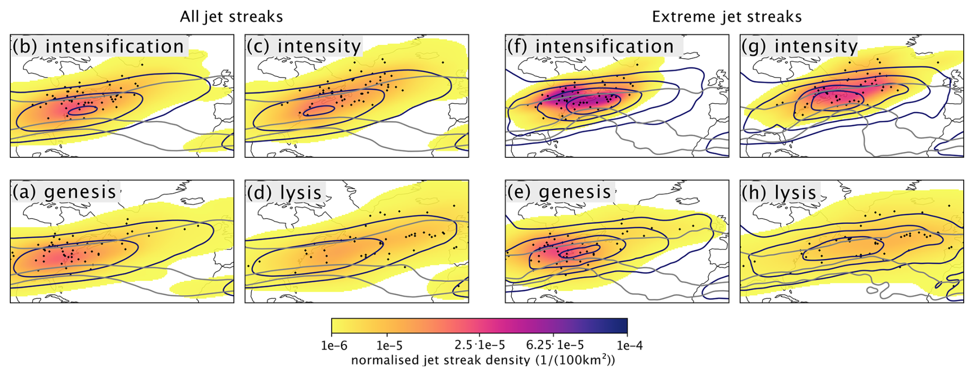
Figure 12 Propagation of (a–d) all and (e–h) extreme North Atlantic jet streaks. The normalized jet streak centre probability density function (PDF) in (100 km²)⁻¹ is in colours (see Sect. 2.1 for a description of how this is computed). The mean PV field (computed like the mean PV gradient fields in Fig. F1 based on PV fields on the 330 K isentrope for all jet streaks and on the 332 K isentrope for extreme jet streaks) is in thick grey contours at 1, 2, and 5 PVU, and the mean wind speed is computed like the PV fields explained above (in thick purple contours every 10 m s⁻¹ starting at 30 m s⁻¹). Black dots represent the centres of extreme jet streaks and are identical in panels (a)–(d) and (e)–(h). For each group of jet streaks, the four panels show the times of (a, e) genesis, (b, f) peak intensification, (c, g) peak intensity, and (d, h) lysis. This order (clockwise starting with the bottom left) was chosen to have the time of peak intensification and intensity in the top row.

Figure 12 illustrates the evolution of the North Atlantic jet streaks during the four stages of a jet streak lifetime. At jet streak genesis (Fig. 12a), most centres are located upstream of the Gulf Stream sector and above the continental USA. As jet streaks intensify, they generally propagate northeastward (Fig. 12b, c). At peak intensification, the variability in jet streak centre positions remains comparatively low, and a marked maximum in their occurrence frequency is over the east coast of the USA and the Gulf Stream. Despite the northeastward propagation of jet streaks during their life cycle, the averaged wind speed and PV exhibit minimal change during the four stages of a jet streak life cycle (grey and purple contours in Fig. 12a–d). This indicates a significant case-by-case variability over the large scale during jet streak life cycles and motivates a jet-streak-centred analysis, which is presented below.

Reducing the sample to extreme jet streaks leads to greater consistency between the evolution of jet streak centre positions, the mean PV contours, and the mean wind speed (Fig. 12e–h). Extreme jet streak centres are more spatially concentrated compared to those of all jet streaks, especially during intensification (Fig. 12a–c, e–g). They propagate northeastward, the maximum of the mean wind field increases during the intensification phase (see the emergence of a fourth purple contour, corresponding to 60 m s⁻¹, in Fig. 12f, g), and a small PV ridge at the time of peak intensification emerges in the composite (grey contour in Fig. 12f). Nevertheless, the large sample variability complicates the interpretation and necessitates an object-centred analysis.

We expand the analysis of the mean large-scale flow during the four stages of the jet streak life cycle using an additional separation into the three jet regimes at jet streak genesis (Sect. 2.2.1). Figure B1 shows a clearer separation of the large-scale flow, but the case-by-case jet streak variability within each regime remains large. This indicates that the separation into the three jet regimes is not effective at reducing case-by-case variability to a point that allows the identification of different jet streak life cycles. However, the evolution and occurrence frequency of the different jet regimes during the four stages of a jet streak life cycle warrant further investigation.

3.3 Jet regime occurrence during jet streak life cycles

To explore the link between the jet regimes and the jet streak life cycle, in particular with respect to the intensification of extreme jet streaks, we first analyse the prevalence of the three regimes at the time of peak jet streak intensity. To contextualize the prevalence of each regime, we also evaluate the likelihood of the jet regimes climatologically (white bars in Fig. 13).

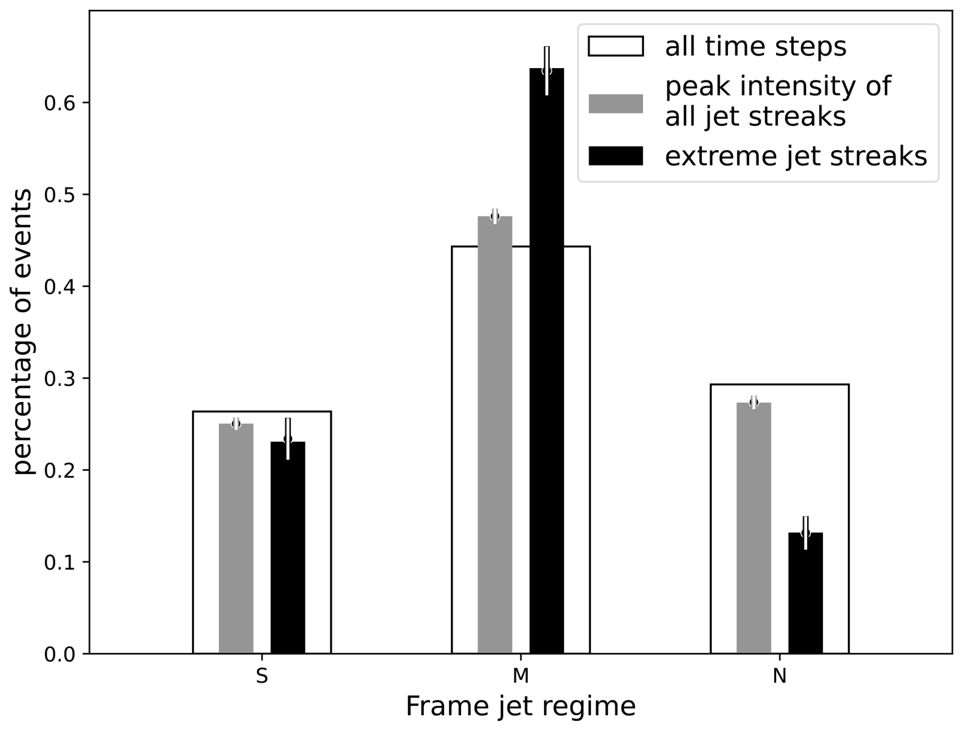
Figure 13 Frequency of times with the jet residing in the S, M, and N regimes. Bars show the frequencies based on all 6-hourly DJF time steps between 1979 and 2023 (wide white), grey is the bootstrapping of time steps of peak jet streak intensity (1050 time steps), and black shows the bootstrapping of time steps of peak jet streak intensity for extreme jet streaks (in total 92 time steps). The heights of the grey and black bars indicate the mean frequency of all resamples, and the vertical grey/white lines indicate the standard deviations of the frequency.

Based on all jet streaks (grey bars in Fig. 13), we find a slight underrepresentation of S- and N-regime jet streaks and a slight overrepresentation of M-regime jet streaks compared to the climatological frequencies. This tendency is accentuated for extreme jet streaks (black bars in Fig. 13), of which 65 % peak in the M regime, while the likelihood of N-regime extreme jet streaks is roughly halved compared to all jet streaks. A bootstrap analysis using 1000 resamples of all events and extreme events (dots and vertical lines in Fig. 13) shows that the increased prevalence of the M regime is a robust result of the analysis. While the same is true for the underrepresentation of the N regime, the climatological likelihood of the S regime is not altered significantly compared to the climatology for both jet streak groups analysed.

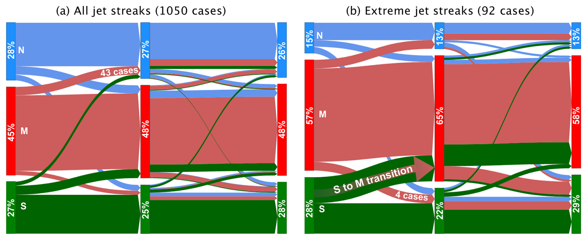
Figure 14 Occurrence of and transitions between the three jet regimes (green S, red M, and blue N) as jet streaks evolve from genesis (left vertical bar) to maximum intensity (middle bar) and lysis (right vertical bar) for (a) all and (b) extreme jet streaks. For example, we find an S regime for 28 %, an M regime for 45 %, and an N regime for 27 % of all jet streak genesis time steps. Arrows indicate the transitions between different jet regimes, and the width of the arrows scales with the number of jet streaks that undergo the corresponding regime transition. For example, of all jet streaks with genesis in the M regime, 43 cases shift to the N regime by the time of peak jet streak intensity in (a). Arrow colours correspond to the regime at genesis.

Figure 14a shows occurrence and transition probabilities of jet regimes at three key moments during the life cycle of a jet streak. Persistence is a key feature in both extreme and non-extreme jet streak evolution, meaning that the eddy-driven jet typically remains within the Frame regime of jet streak genesis (Fig. 14a, b). For jet streaks during whose evolution different Frame regimes occur, the following results are worth noting: starting with the regime at genesis (27 %, 45 %, and 28 % in S, M, and N regimes, respectively) there is a larger tendency for the S regime to shift to the M regime and from the M to the N regime during the intensification period of a jet streak, which is in agreement with the storm track life cycle argument presented in Ambaum and Novak (2014). At lysis, the relative numbers are fairly similar to the values at genesis, and M is the most persistent regime. For the extreme jet streaks, a notable difference is found (Fig. 14b). The probability of a jet streak originating in the S regime subsequently transitioning into the M regime during intensification is 46 %. This is approximately double the climatological transition probability. Additionally, extreme jet streaks are most likely to occur in the M regime. During the decay period, there is a greater number of cases where the S regime transitions to the M regime and vice versa, although there is a relatively low number of instances where the N regime is reached. The increased occurrence of the M regime and increased S-to-M transitions during jet streak intensification align with the oscillator model for the North Atlantic storm track life cycle (Ambaum and Novak, 2014). According to this model, baroclinicity is accumulated when the jet is in the S regime, thereby fuelling the potential for strong baroclinic growth. Consequently, baroclinic growth results in an increased eddy momentum transport, thereby intensifying the eddy-driven jet as it transitions into the M regime. The jet is typically strongest in the M regime, which increases the likelihood of the occurrence of extreme jet streaks.

3.4 Jet-streak-centred composites

This section explores composites of jet-streak-centred wind and PV fields. We start with the PV gradient and wind speed at the time of peak intensity for non-extreme (Fig. 15a) and extreme jet streaks (Fig. 15b). The PV gradient fields in both display a Rossby wave with a wavelength of about 6700 km. The jet streak centre is located at a ridge crest and is anticyclonically curved. Extreme jet streaks (Fig. 15b) display an advanced stage of PV streamer formation downstream. Maximum wind speed for extremes is on average 102.8 m s⁻¹, compared to 87.3 m s⁻¹ for non-extreme cases.

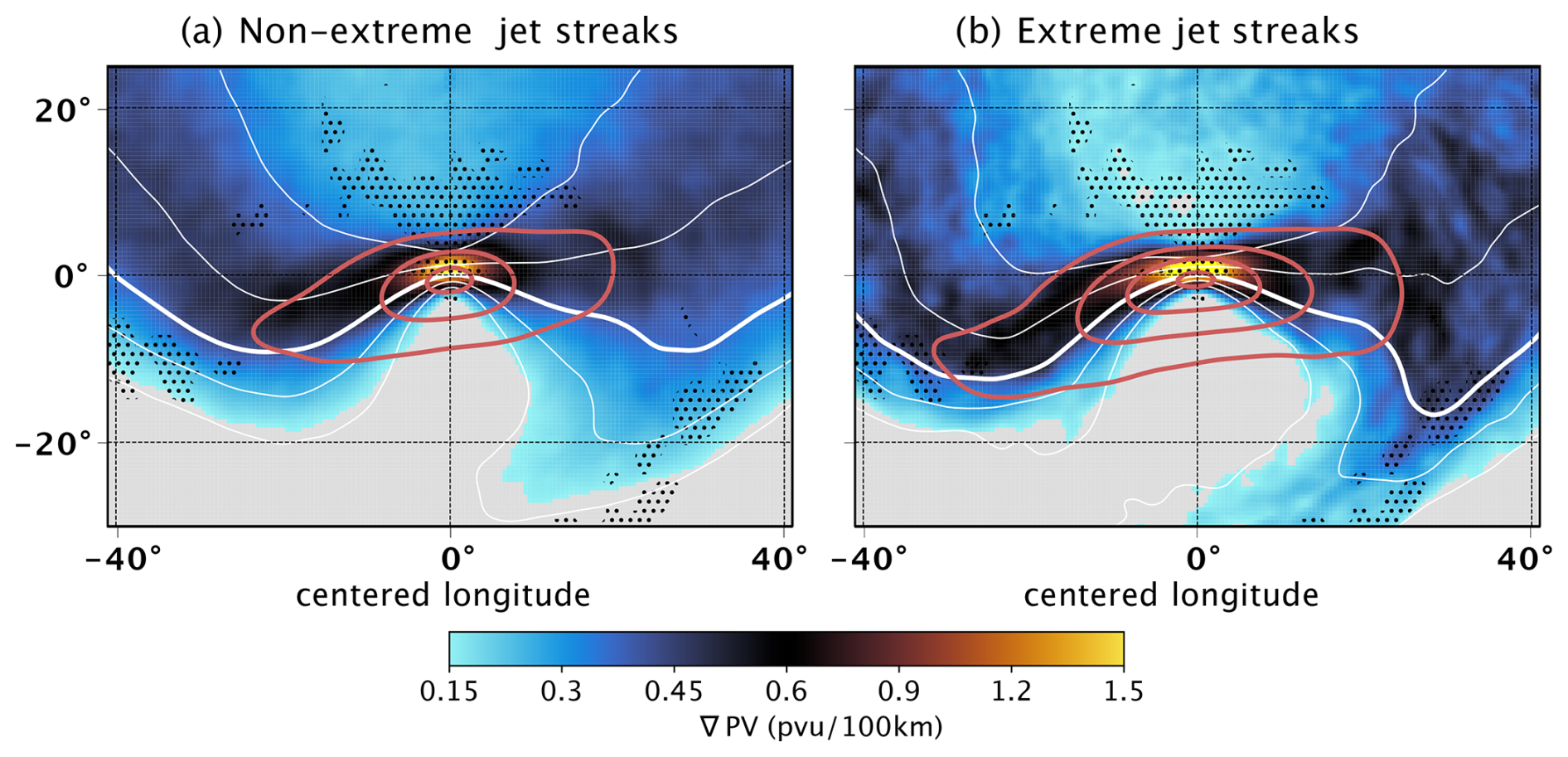
Figure 15 Jet-streak-centred composites based on bootstrapping of (a) non-extreme jet streaks and (b) extreme jet streaks at the time of peak intensity. Shown is the mean of the norm of the PV gradient on the central jet streak isentrope (colours); values smaller than 0.15 PVU (100 km)⁻¹ are white. Contours show the mean PV for $[\mathrm{0.5},\mathrm{1.0},\mathrm{4.0},\mathrm{6.0}]$ PVU (white) and 2 PVU (bold white contour) on the central isentrope and the mean of wind speed on the central isentrope (red) every 20 m s⁻¹, starting at 40 m s⁻¹. Stippling shows where the difference between the means of the mean of the norm of the PV gradient on the central jet streak isentrope of non-extreme and extreme jet streaks based on 1000 resamples is larger than the standard deviation of the means of both categories combined.

The maximum PV gradient is located slightly poleward of the wind speed maximum (Fig. 15a, b), in accordance with the theoretical predictions set forth in Bukenberger et al. (2023). The PV gradient maximum is flanked by a minimum on the tropospheric side and a local minimum on the stratospheric side, which is more pronounced in extreme cases. While the standard deviation in the PV gradient composite is relatively small compared with the mean value in the centre (Fig. C1a), both are of a similar order of magnitude up- and downstream of it. This indicates that the intensity of jet streaks is at its maximum when centred on the ridge of a Rossby wave. However, the exact positions along the ridge and the shape of the Rossby wave can vary considerably (Fig. C1b). This extensive variability in the composites, which is observed on a case-by-case basis, motivates the implementation of a more detailed clustering approach.

3.4.1 Jet-streak-centred SOM clusters

We cluster jet streaks based on jet-streak-centred PV fields at the times of peak intensification and intensity, as detailed in Sect. 2.2. We aim for low similarity between clusters, which imposes an upper limit on the number of clusters. At the same time, we aim to keep clusters with clearly different Rossby wave patterns and concentrations of extreme jet streak events separate. Balancing these two goals yields six clusters, composites of which are shown in Appendix G. All clusters share some interesting commonalities (Fig. G4):

1. Their composites show either anticyclonic or no Rossby wave breaking at the time of both peak jet streak intensification and intensity. The tropopause is either straight or anticyclonically curved at the jet streak centre at the time of peak jet streak intensity (second, fourth, and sixth rows in Fig. G4).

2. At time of peak jet streak intensity, all cluster composites show the jet streak centre in the ridge of the Rossby wave, never in a trough (second, fourth, and sixth rows in Fig. G4).

3. Between the times of peak intensification and intensity, the jet streak centre either remains stationary with respect to the Rossby wave or propagates downstream. Moreover, the amplitude of the composite Rossby wave grows along with the jet streak intensity between the time of peak jet streak intensification and intensity (first vs. second, third vs. fourth, and fifth vs. sixth rows in Fig. G4).

Clusters for which this growth is most pronounced (cluster 1 and cluster 2, referred to as C1 and C2 in the following; compare temporal evolutions in Fig. G4a–h to those in Fig. G4i–x) feature the largest fractions of extreme jet streaks: 24 out of 126 anticyclonically oriented jet streaks (19.0 %) and 29 out of 197 zonally oriented jet streaks (14.7 %) are extreme cases. Complementary to that, the clusters with the smallest changes in Rossby wave amplitude (C3 and C4; see Fig. G4i–o) have the smallest mean peak jet streak intensity, and each contains a fraction of less than 5 % of all extreme jet streaks.

Table 2 Characteristic properties of the different SOM clusters. The number of jet streaks as well as extreme jet streaks in each cluster is mentioned, along with the percentage that they constitute within the cluster (for example, 19 % for cluster 1, containing a total of 126 events with 24 extreme events). The clusters with a bold font are those with a southwest–northeast orientation and with composites showing anticyclonic wave breaking at the time of peak jet streak intensity.

Comparing the climatological occurrence frequency of the three Frame jet regimes with their frequency in each cluster shows that strong anticyclonic wave breaking coincides with high frequencies of M and N regimes (for example C1) and more zonal Rossby waves with more frequent S regimes (for example C3 and C6) (Table 2).

The clusters differ in the position of the jet streak centre along the Rossby wave ridge and consequently in the orientation of the jet streak (Fig. G4). In C1, C4, and C5 (highlighted bold in Table 2), the jet streak centre is positioned upstream of the ridge axis (Fig. G4a–d, m–t). The jet streaks in those clusters are oriented southwest–northeast, while the composite Rossby wave shows signs of anticyclonic wave breaking. The stronger the wave breaking of a cluster, the higher the fraction of extreme jet streaks (e.g. 19 % in C1 vs. 2.4 % in C4). Two clusters (C2, C3) have the jet streak centre positioned slightly downstream of the ridge axis at peak intensity, and the streaks are either zonal (extremes in C2) or oriented northwest–southeast (C3 extremes) (Fig. G4e–l). Cluster C2 contains the plurality of extreme jet streaks, with 29 out of 91 events (14.7 % of the jet streaks in C2 are extreme). Finally, C6 shows a weak Rossby wave with the centre of the straight and zonally oriented jet streak at the Rossby wave crest and with little intensification between the times of peak intensification and intensity (Fig. G4u–x).

The large prevalence of southwest–northeast-oriented jet streaks is consistent with Clark et al. (2009), who showed that over the North Atlantic, most jet streaks are southwesterly. Studies of jet streaks in other regions, particularly the eastern North Pacific, show more northwesterly jet streaks, so our clusters are domain- and season-specific to the North Atlantic winter.

We focus in the following on C1 and C2, which have both the largest frequencies of extreme jets and clearly distinct large-scale circulations. We refer to the former as mostly anticyclonic cases and to the latter as zonal cases. For completeness, an analysis of all clusters is shown in Appendix G.

3.4.2 Zonally and anticyclonically oriented jet streak clusters

We start with the Rossby wave patterns in Fig. 16. All anticyclonically oriented jet streaks (C1) intensify upstream of the crest of the Rossby wave, downstream of which we find a pronounced PV streamer. Higher PV gradients at the jet streak centre of extreme cases are a robust feature in bootstrapping analysis (see stippling in Fig. G5a vs. b, c vs. d). The PV streamer in the extreme jet streak composite grows and bends more anticyclonically between the times of peak jet streak intensification and intensity (also robustly; see stippling in Fig. G5a vs. b, c vs. d). This indicates stronger anticyclonic wave breaking for extreme jet streaks (Fig. 16a–d). C1 jet streaks tilt southwest–northeast at both times and turn to be more zonal as they approach the Rossby wave crest at the time of peak intensity.

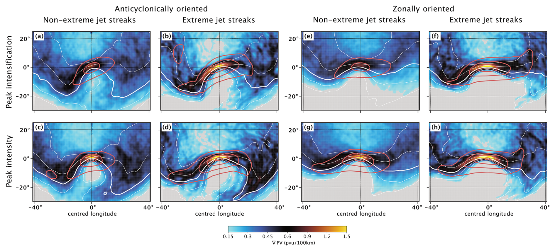
Figure 16 Jet-streak-centred composites based on (a–d) anticyclonically oriented jet streaks and (e–h) zonally oriented jet streaks. Panels (a), (b) and (e), (f) show composites at the time of peak intensification for (a, e) non-extreme and (b, f) extreme jet streaks. Panels (c), (d) and (g), (h) show the time of peak jet streak intensity for (c, g) non-extreme and (d, h) extreme jet streaks. Colours are the PV gradient (PVU (100 km)⁻¹); values smaller than 0.15 PVU (100 km)⁻¹ are grey. The contours are as follows: white – mean PV on the central isentrope, with thick lines indicating 2 PVU and thin lines $[\mathrm{0.5},\mathrm{1.0},\mathrm{4.0},\mathrm{6.0}]$ PVU; red – wind speed on central isentrope every 20 m s⁻¹, starting at 40 m s⁻¹.

Composites of zonal jet streaks (C2) show a pronounced Rossby wave and zonally oriented composite jet streak at its crest but no PV streamer downstream at the time of peak jet streak intensification. A PV streamer develops until the time of peak intensity. Extreme jet streaks feature more pronounced troughs and PV streamers than non-extreme jet streaks at the time of peak intensity (Fig. G1e–h). However, the composite Rossby wave does not bend anticyclonically for either subset of zonally oriented jet streaks. Note that for both clusters, the average increase in maximum wind speed between the times of peak intensification and intensity is similar for non-extreme and extreme jet streaks (∼ 20 m s⁻¹). The difference in peak intensity stems from already higher intensities of extreme jet streaks at the time of peak intensification.

The maximum of the composite PV gradient and the stratosphere-ward displacement of bands of high PV gradients with respect to the wind speed maximum increase with jet streak intensity for both clusters and all jet streaks (Fig. 16a, b vs. c, d and Fig. 16e, f vs. g, h), as is expected from theory. Another robust difference between extreme and non-extreme jet streaks is the more narrow region of enhanced PV gradients close to the jet streak axis for extreme cases (Fig. 16, first vs. second and third vs. fourth columns).

The PV gradient standard deviation shows more large-scale variability in anticyclonically than zonally oriented jet streaks (Fig. G1a–d vs. e–h). Most of the PV gradient variability can be attributed to the variability in the exact shape of the Rossby wave on which the jet streak evolves and the jet streak centre position relative to it. The variability increases as jet streaks reach peak intensity, especially for anticyclonically oriented jet streaks and especially upstream of the jet streak centre (Fig. G1). The standard deviation of PV gradients far away from the jet streak centre of extreme jet streaks is larger than that of non-extremes but notably smaller close to it for both clusters (e.g. Fig. G1a vs. b and Fig. G1c vs. d). This reduced variability indicates that the large PV gradient at extreme jet streak centres is a robust feature.

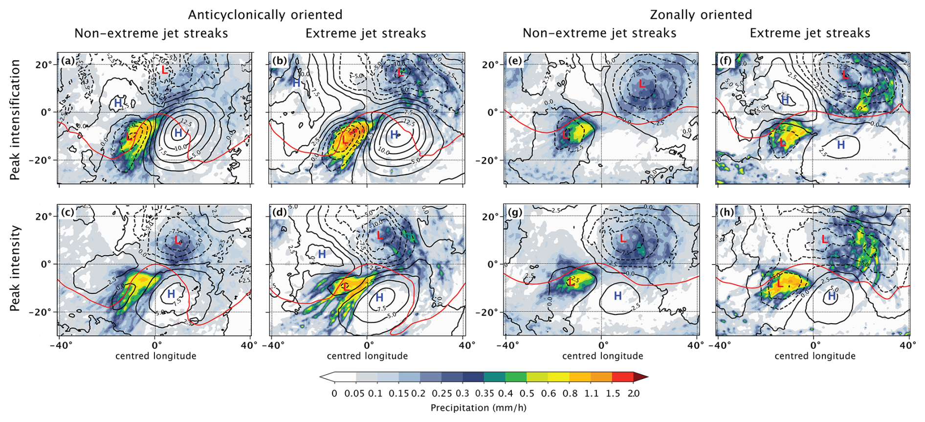
Figure 17 Jet-streak-centred composites for anticyclonically oriented jet streaks (first two columns) and zonally oriented jet streaks (last two columns). The top row shows the time of peak intensification and the bottom row the peak intensity. Each set of four panels is divided into non-extreme (first and third column) and extreme (second and fourth column) jet streaks. Shading is the hourly precipitation (mm h⁻¹). The contours are as follows: black – mean sea level pressure anomaly with respect to the 1979–2023 winter climatology every 2.5 hPa, with negative values shown with dashed contours; red – mean PV on the central isentrope at 2 PVU.

Next, consideration is given to lower tropospheric levels for anticyclonically oriented jet streaks (Fig. 17a–d). At the time of peak jet streak intensification, the mean sea level pressure (SLP) anomaly shows a strong and anticyclonically oriented high-pressure system below the right jet exit, which weakens until peak jet streak intensity. An intense and large cyclone is located to the north of the strong anticyclone, below the left jet exit. A second, smaller negative SLP anomaly is located below the right entrance at peak jet streak intensification but merges with the cyclone in the left exit by the time of peak jet streak intensity, where only one cyclone remains.

It is more intense for extreme jet streaks and exhibits an SLP pattern typical of anticyclonic wave breaking (Thorncroft et al., 1993). This is consistent with the dominance of M- and N-regime jet streaks in the anticyclonic cluster (93 %). Since both high- and low-pressure anomalies are stronger for extreme cases, the average meridional pressure gradient between the two systems is about 30 % stronger for the composite of extreme cases (Fig. G2c vs. d). The cyclone is associated with an elongated southwest–northeast oriented band of enhanced precipitation along its cold front whose intensity changes only marginally between the times of peak intensification and intensity (Fig. 17a–d). The maximum in cold-frontal precipitation is located below the right jet entrance and is robustly more intense for extreme jet streaks (compare the first vs. second column in Fig. 17 and see stippling in Fig. G2a–d).

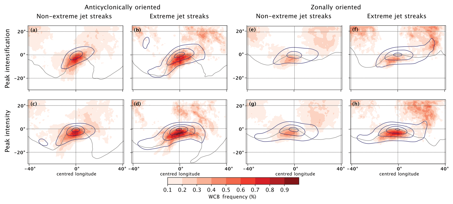
Figure 18 Jet-streak-centred composites for anticyclonically oriented jet streaks (first two columns) and zonally oriented jet streaks (last two columns). The top row shows the time of peak intensification and the bottom row the peak intensity. Each set of four panels is divided into non-extreme (first and third column) and extreme (second and fourth column) jet streaks. Colours show the WCB outflow frequency at 400 hPa. The contours are as follows: grey – mean PV on the central isentrope at 2 PVU; blue – mean of wind speed on the central isentrope every 20 m s⁻¹, starting at 40 m s⁻¹.

To relate these results to the previous literature on cross-isentropic mass flux in warm conveyor belts (WCBs), WCB frequencies at 400 hPa (Fig. 18a–d) complement the analysis of low-level dynamics. They show little change during the lifetimes of non-extreme anticyclonically oriented jet streaks. Most WCB outflow occurs on the tropospheric side of the jet axis. The left jet exit, which exhibits slightly stronger precipitation, also shows more WCB outflow for extreme jet streaks. Consistent with the precipitation patterns, WCB outflow feeding into the Rossby wave ridge is more frequent for extreme than non-extreme jet streaks (Fig. 18a, c vs. b, d) and exceeds 80 % at grid points close to the Rossby wave crest as jet streaks reach peak intensity. Robust differences between the WCB outflow of extreme and non-extreme C1 jet streaks are already given at the time of peak jet streak intensification but increase as they reach peak intensity (Fig. G6a–d).

In the cluster of zonally oriented jet streaks (C2), the positive SLP anomaly intensifies between peak jet streak intensification and intensity and approaches the jet streak centres below the right jet exit (Fig. 16e–g). A mature cyclone resides below the left jet exit, and the cyclone–anticyclone pair appears more meridionally aligned for extreme cases. In the warm sector of this cyclone, the precipitation rate for extreme jet streaks is approximately double that of non-extremes, and this result is robust against resampling (Fig. G2e–h). The pressure difference within the cyclone–anticyclone pair is roughly 45 hPa during peak jet streak intensity, compared to 20 hPa for non-extreme cases, and is driven by both stronger cyclones and anticyclones for extreme cases (Fig. G2e–h).

The most remarkable difference in the synoptic situation between the clusters of zonally and anticyclonically oriented jet streaks is the continued presence of a second, mesoscale surface low below the right jet entrance of zonally oriented jet streaks. It weakens for non-extreme cases but grows for extreme jet streaks. Precipitation increases as jet streaks reach peak intensity, again with robustly more precipitation in extreme jet streak composites. For anticyclonic cases, no upstream cyclone is found at peak jet streak intensity.

Similar to the anticyclonic cluster, WCB outflow on the tropospheric side of the jet is more frequent for extreme zonally oriented jet streaks (Fig. 18a–d vs. e–h), but the difference only becomes statistically robust at the time of peak jet streak intensity (stippling in Fig. G6e–h). By this time, the WCB frequency in this region more than doubles for extreme jet streaks (Fig. 18e–h). WCB outflow in the left jet exit is very rare for non-extreme zonally oriented jet streaks but more frequent for extreme cases, indicating enhanced cross-isentropic mass flux, as is expected from more intense precipitation rates.

4 Conclusion and outlook

This study analyses the evolution of North Atlantic winter (DJF) jet streaks from January 1979 to February 2023 using 6-hourly ERA5 data. The analysis is based on an object-centred identification and tracking framework, identifying jet streaks based on the isentrope of maximum wind speed. The proposed method ensures robust identification of jet streaks, independent of their varying heights. We first investigate basic characteristics of North Atlantic winter jet streaks and later combine the results with object-centred composites to study jet streak life cycles in various flow situations. To investigate the connection between jet streaks and the eddy-driven jet stream, the results are categorized based on the jet stream regimes defined by Frame et al. (2011). Furthermore, the study groups jet streaks into different clusters based on isentropic PV using a self-organizing map algorithm in an attempt to establish a link between jet streaks and different phases of Rossby wave development. To the best of our knowledge, this is the first systematic comparison of extreme and non-extreme jet streaks, and the results indicate that extreme jet streaks can develop in association with different weather systems but are always developing under an increased influence of diabatic processes. The following sections discuss the most important findings of this study in more detail, point out key limitations, and lay out a possible avenue for future research.

4.1 Characteristic properties of extreme North Atlantic winter jet streaks

The peak intensity of North Atlantic wintertime jet streaks is 87 ± 9 m s⁻¹ (103 ± 4 m s⁻¹ for extreme jet streaks). The maximum wind speed reached during a jet streak life cycle correlates with the maximum PV gradient and the lifetime of events, which is 1.3 times longer for extreme than for non-extreme jet streaks. We find that extreme jet streaks are distinguished by a prolonged strengthening period as well as increased intensification rates. Jet streaks propagate across the North Atlantic from southwest to northeast throughout their life cycle, and extreme jet streaks tend to propagate larger distances during their intensification, which is in agreement with their prolonged intensification period.

Categorizing jet streaks based on the Frame jet regimes at the time of peak jet streak intensity shows that the frequencies of the three jet regimes, which are intricately linked to the state of the North Atlantic storm track (Frame et al., 2011; Woollings et al., 2010), are similarly distributed at peak jet streak intensity as they are climatologically. With Frame et al. (2011), we follow a line of research that finds three jet regimes based on vertically and zonally averaged wind profiles using K-means clustering. The ideal number of regimes could change with the reanalysis dataset at hand, other methods for jet detection and profile computation, and the validity indices chosen to evaluate the K-means clustering. Follow-up studies involving other state-of-the-art atmospheric reanalysis products such as JMA's JRA-55 and NASA's MERRA-2 (Kobayashi et al., 2015; Gelaro et al., 2017) and different methods to identify low-level jet regimes would help solidify our understanding of upper- and lower-level interaction in jet streak evolution. This finding suggests that a finer-grained clustering of jet streaks is needed to understand their variability from case to case. A notable exception is the increased occurrence frequency of the central jet regimes (M regimes) during times of extreme jet streaks. Also, the transition from an equatorward to a central jet regime (S to M) occurs with increased probability during extreme jet streaks. This suggests that the enhanced baroclinicity normally observed during S regimes leads to strong baroclinic development, which might be conducive to the sustained intensification period characteristic of extreme jet streaks.

4.2 Large-scale flow situation during jet streak evolution

A self-organizing-map (SOM) algorithm combined with hierarchical agglomerative clustering of upper-level PV results in six clusters, which display the following main characteristics:

1. At the time of peak jet streak intensity, the jet streak centre is always located close to the axis of a Rossby wave ridge. This result is in line with theory because the combination of the pressure gradient and centrifugal forces balance the Coriolis force to yield a super-geostrophic wind in a ridge. The jet streak is located slightly upstream of the ridge crest of anticyclonic Rossby waves and at the ridge crest of the zonally oriented Rossby wave axis during peak intensification and at peak intensity.

2. No cluster mean exhibits well-marked cyclonic Rossby wave breaking at the times of peak intensification or peak intensity.

The two clusters that contain the majority of extreme jet streaks are investigated in more detail, with a focus on the time of peak jet streak intensity. The first cluster is anticyclonically oriented, with 24 extreme jet streaks out of 126 total events. The second cluster is zonally oriented and contains a total of 197 (29 extreme) events. Anticyclonically curved jet streaks form on a Rossby wave with strong anticyclonic wave breaking. The jet streak centre is located upstream of the ridge axis at peak intensity. A mature cyclone centred poleward of the left jet exit is present in the low-level composites for anticyclonically oriented jet streaks. The precipitation below the right jet streak entrance is associated with the elongated upstream extension of the cold front attending the mature extratropical cyclone in the left exit. For zonally oriented jet streaks, we find a mature Rossby wave in upper-level PV composites that intensifies along with the jet streak. The jet streak centre is co-located with the axis of the Rossby wave ridge at the time of peak jet streak intensity. At the surface near the left jet streak exit, a mature extratropical cyclone is identified. It is accompanied by warm-sector precipitation, which is more intense for extreme than non-extreme jet streaks. In contrast to the single cyclone below the left exit of anticyclonically oriented jet streaks, this cluster shows an additional, smaller mesoscale cyclone beneath the right jet streak entrance, which produces intense precipitation. The warm-conveyor-belt outflow that is associated with this low-pressure system feeds the upper-level ridge.

The two clusters have different upper-level Rossby wave patterns and lower-level weather systems but share key characteristics, particularly in the differences between extreme and non-extreme jet streaks. Composites based on extreme events show larger Rossby wave amplitudes and higher warm-conveyor-belt outflow frequencies for both clusters. The low-level circulation is characterized by an anticyclone southeast of the jet streak centre and a strong cyclone below the left jet exit. Precipitation is more intense in extreme cases, in line with the increased cross-isentropic motion in the rising warm conveyor belt. The composites also indicate the important role of an anticyclone located below the right jet streak exit.

4.3 Limitations of jet streak detection

The jet streak tracking algorithm has two key limitations: first, its restricted domain, and second, the fact that it detects only one jet streak centre at a time.

Confinement to the North Atlantic domain leads to inaccuracies in capturing the genesis and lysis of jet streaks as they reach the domain boundary. We estimated the effect of this limitation by identifying jet streaks with genesis or lysis near the boundaries of the North Atlantic domain and compared their lifetimes to jet streaks that reside well within the domain throughout their evolution (Fig. D1). The results indicate that primarily strong and long-lived jet streaks are affected by the domain boundaries, such that this limitation mainly affects the longest life cycles. Moreover, jet streaks that start (end) by entering (leaving) the domain typically reach their strongest intensification and intensity well within the domain, such that this limitation does not seem to affect those key life cycle stages.

Detecting only one jet streak at a time runs the risk of missing weak jet streaks while stronger ones are present, potentially biasing weak jet streaks towards shorter durations or missing them altogether. We compared the lifetimes of jet streaks whose genesis or lysis happens directly after the lysis or before the genesis of another jet streak in the domain to the lifetimes of jet streaks for which this is not the case. Since both groups have similar lifetime distributions and mean intensities (Fig. D1), the link between jet streak intensity and duration is unlikely to be caused by this method limitation.

We believe that for the focus of this study – peak jet streak intensification and intensity – neither the domain boundaries nor the inability to track multiple concurrent jet streaks will meaningfully impact our findings. A more flexible algorithm allowing for multiple concurrent jet streaks is currently in development and will be used in follow-up studies.

4.4 Outlook

Diabatic processes play an increased role in extreme jet streaks, a result that has important implications for numerical modelling and the predictability of these events. A warmer and therefore more humid atmosphere has more potential for diabatic heating of clouds, and increased diabatic heating has been pinpointed as a key driver of the recent jet stream intensification (Hermoso et al., 2024). Understanding the role of diabatic PV modification in the evolution of jet streaks is therefore also important for shaping our expectations of trends in the frequency and intensity of extreme jet streak events in a warming climate. Our next step is therefore to perform a detailed quantitative analysis of the influence of diabatic processes on jet streak intensification and, in particular, on extreme jet streaks. Such an analysis is the focus of the next part of this study, which uses the Lagrangian PV gradient framework for jet streak evolution. The framework has proven useful when quantifying the role of diabatic processes on jet streak dynamics in case studies (Bukenberger et al., 2023), and combining it with jet-streak-centred composites over a reanalysis data period will improve the mechanistic understanding of diabatic–adiabatic coupling in jet streak dynamics.

Appendix A: Evolution of central isentrope

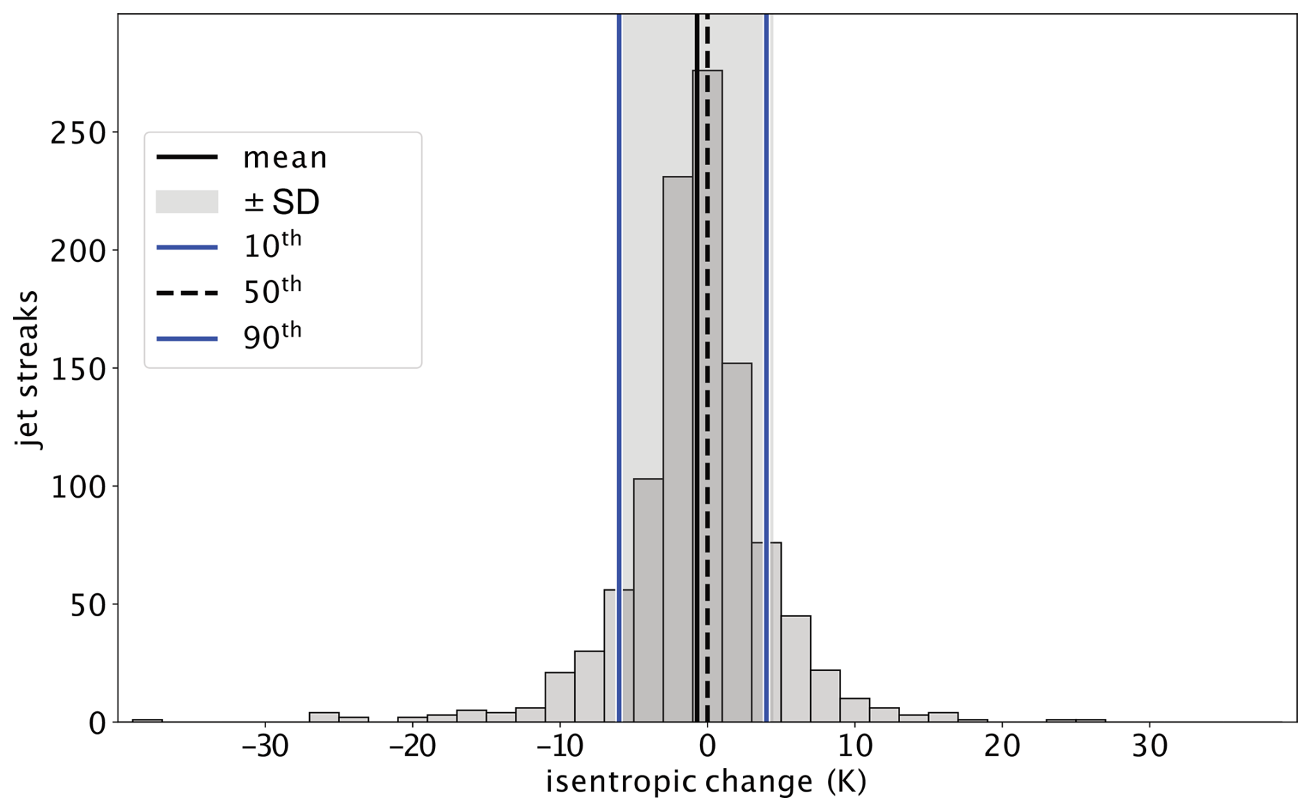
Figure A1 Changes in the instantaneous central jet streak isentrope between the time of peak jet streak intensification and peak jet streak intensity for the 1050 North Atlantic winter jet streaks. Grey bars are the histogram; vertical lines show the mean (solid black), median (dashed black), and 10th and 90th percentiles (blue; −4 and +6 K, respectively) of the distribution.

Appendix B: Jet streak paths over the North Atlantic

To understand the extent to which the variability in jet streak paths can be explained by the eddy-driven jet, we compiled normalized jet streak centre PDFs over the North Atlantic for S-, M-, and N-regime jet streaks. Figure B1 shows that jet streaks in all regimes tend to evolve from southwest to northeast. Figure B1a–d illustrate the paths of S-regime jet streaks, which are predominantly zonal. Notably, and consistent with their longer lifetimes (Sect. 3.1), extreme jet streaks in this category tend to propagate farther eastward compared to average S-regime jet streaks (Fig. B1b–d). The composite wind speed and PV fields remain qualitatively unaltered throughout S-regime jet streak evolution.

M-regime jet streaks propagate northeastward, and most of them reach peak intensity at their northernmost position. The composite jet stream intensifies along with them and tilts northeastward throughout their entire evolution. The concurrent intensification of the composite jet stream and M-regime jet streaks is due to a large concentration of jet streak centres in the meridional direction, especially at times of peak intensification and intensity (Fig. B1e–h). The PV composite indicates Rossby wave intensification along with jet streak intensification (grey contours in Fig. B1e–g). N-regime jet streaks are either near-stationary close to the North American east coast or propagate northeastward across the North Atlantic. Some N-regime jet streaks turn southward between the time of peak intensity and lysis, with the PV field indicating anticyclonic wave breaking (Fig. B1i–l). While we find different mean jet streak centre paths for each Frame regime, the variability in jet streak paths for each remains as large as that of all jet streaks. While the normalized PDFs show some signatures of the different jet regimes, the PDFs of all groups are broad, implying that the bulk of variability in jet streak evolution over the North Atlantic cannot be explained by the state of the eddy-driven jet.

Another way to investigate the coupling between lower and upper levels is to compare the mean state of the upper-level jet during peak jet streak intensity in different Frame jet regimes with the lower-level composites.

Figure B2 shows differences in Rossby wave patterns between the upper (328 K) and middle (310 K) levels for S- and N-regime jet streaks. For S-regime jet streaks, the composite jet at upper levels exhibits a westward displacement with respect to the jet at lower levels. For N-regime jet streaks, the Rossby wave pattern at upper levels is less clear compared to the anticyclonic wave breaking at lower levels, probably due to greater variability at upper levels (Fig. B2n vs. l). M-regime jet streaks show consistent Rossby wave patterns at upper and lower levels, suggesting enhanced vertical coupling. This result points toward an increased interaction between upper and lower levels for jet streaks that peak in the M regime and might point toward an increased likelihood of merged jet states in the M regime. It is also consistent with the finding that most extreme jet streaks peak in the M regime and show enhanced lower-level–upper-level coupling.

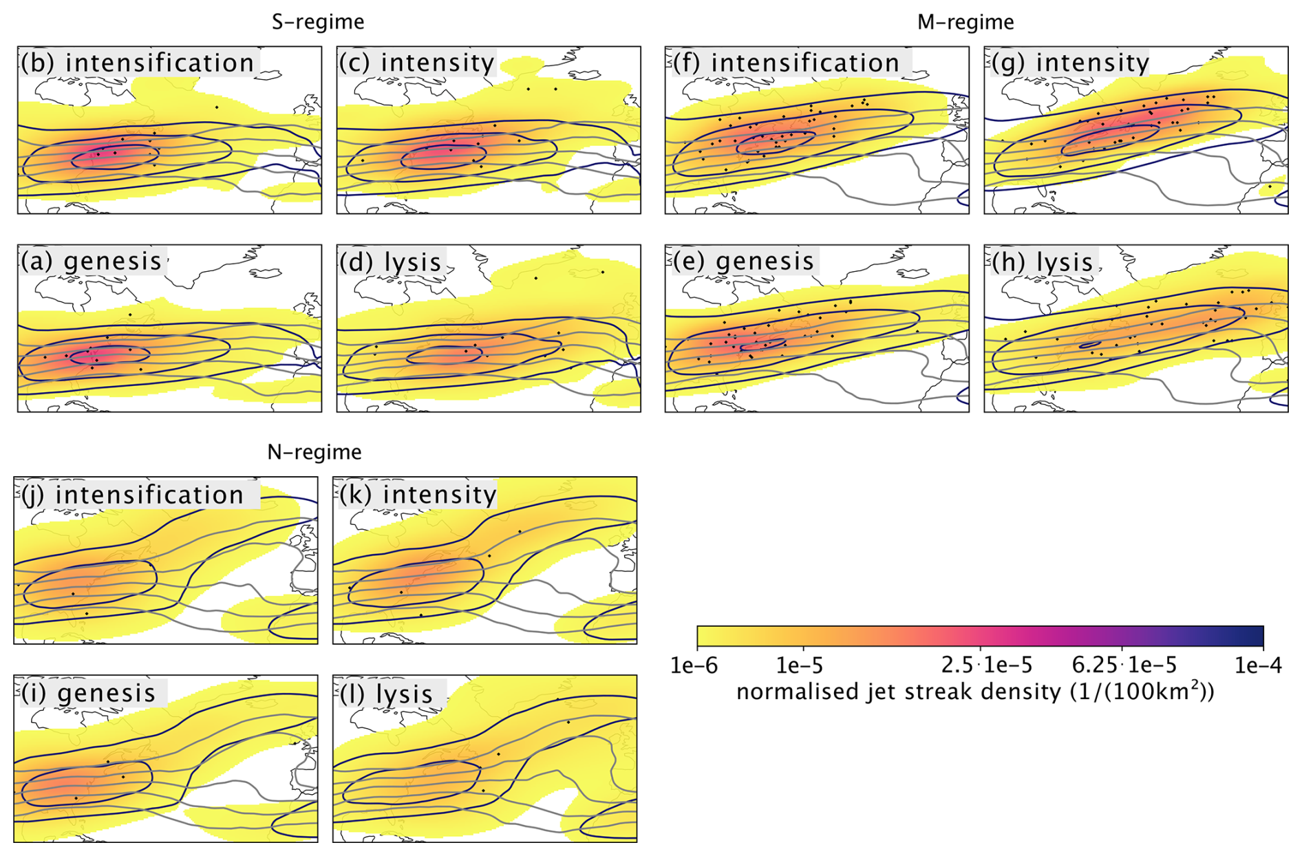
Figure B1 Life cycles of all jet streaks grouped by Frame regime. Like Fig. 12a–d but for the S-regime (a–d), M-regime (e–h), and N-regime (i–l) jet streaks. Grey contours show 330 K PV isolines between 1 and 5 PVU every 1 PVU.

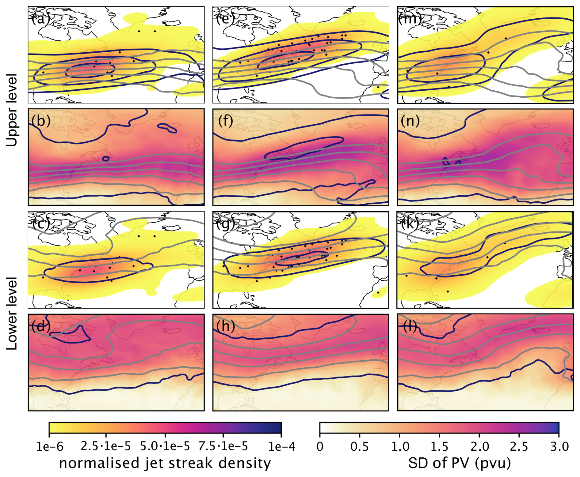
Figure B2 Characteristics of large-scale flow at peak jet streak intensity on the central isentrope (rows 1–2) and at 310 K (rows 3–4) for jet streaks in the S (first column), M (second column), and N (third column) regimes. The first row is like panels (c), (g), and (k)​​​​​​​ in Fig. B1, and the third row is like panels (c), (g), and (k) in Fig. B1 but with PV and wind speed at 310 K instead of 330 K. The second row shows the standard deviation of PV on central jet streak isentropes at the time of peak jet streak intensity (colours) and the standard deviation of wind speed on the central jet streak isentropes at the time of peak jet streak intensity at intervals of 10 m s⁻¹ (purple contours), starting at 10 m s⁻¹. The grey contours are like the grey contours in Fig. B1c, g, and k. The fourth row shows the same variables as the second row but with all variables at 310 K instead of 330 K.

Appendix C: Standard deviation of PV gradients

Figure C1 shows the jet-streak-centred standard deviation of PV gradients and wind speed for non-extreme (Fig. C1a) and extreme (Fig. C1b) jet streaks. It illustrates the variability in the dynamical environment in which jet streaks develop but also shows the utility of the centred composites, as the standard deviation of the PV gradient is low close to the composite jet streak centre. Extreme jet streaks seem to evolve in two clusters, as can be seen by the two regions of enhanced variability in wind speed southwest and northeast of the composite extreme jet streak centres (Fig. C1b). The overall large variability in the large-scale dynamical environment around jet streak centres at peak jet streak intensity motivates the clustering of jet streaks into different dynamical regimes.

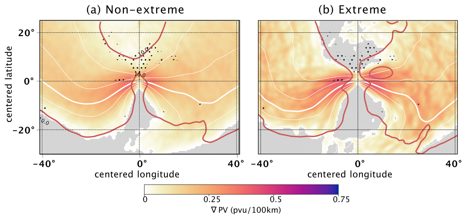
Figure C1 As in Fig. 15 but with the standard deviation of the PV gradient instead of PV. The contours are as follows: white – PV on the central isentrope; red – standard deviation of wind speed on the central isentrope every 10 m s⁻¹, starting at 10 m s⁻¹.

Appendix D: Lifetimes for jet streaks with different characteristics

To test whether the limitations of the jet streak tracking algorithm (i.e. tracking only one object at a time and being limited to the North Atlantic domain) cause biases that call the reliability of our results into question, especially concerning the correlation between peak intensity and the lifetime of jet streaks, we extracted jet streaks with different characteristics that should be affected by those two limitations. Figure D1 shows that, first, jet streaks whose lifetimes are limited by the North Atlantic domain boundary tend to have longer lifetimes than those that stay within the domain throughout their entire evolution (compare dark blue and dark red boxes). The distribution of their peak intensities is also shifted to higher values (not shown). This indicates that, if anything, this limitation leads to an underestimation of the correlation between peak jet streak intensities and lifetimes.

Jet streaks with genesis/lysis directly after/before the lysis/genesis of another jet streak tend to have shorter lifespans than those that emerge without another jet streak beginning/ceasing to exist. However, the difference is marginal compared to the variability in the entire dataset. From these two results, we conclude that while the limitations of the jet streak tracking algorithm cause an overall bias toward shorter lifetimes, the correlation between peak jet streak intensity and lifetime is robust.

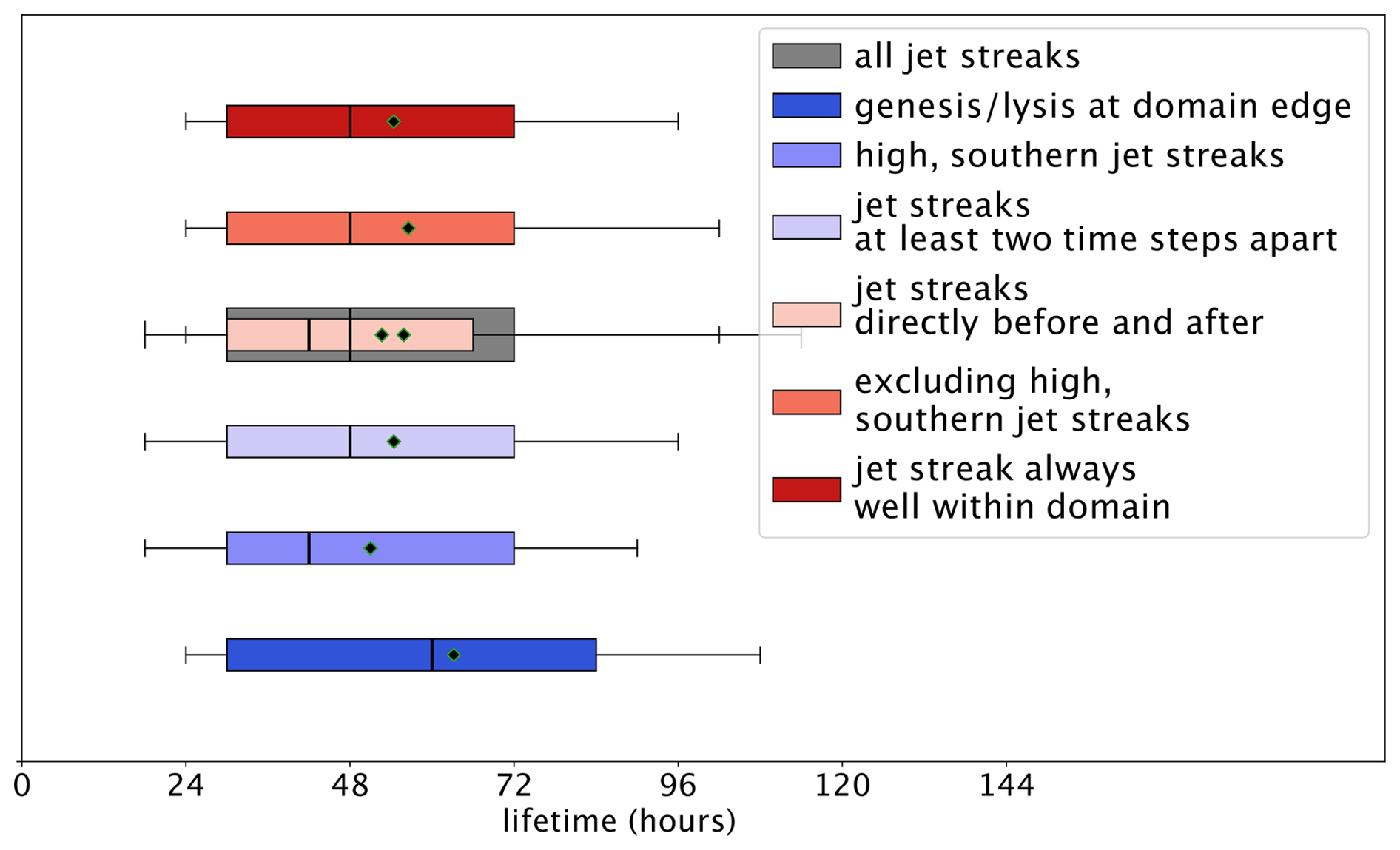
Figure D1 As in Fig. 10 but for jet streaks with different characteristics. Genesis/lysis at domain edge indicates those that begin or end by entering/leaving the North Atlantic domain. Jet streaks always well within domain are all jet streaks except for those that begin or end by entering/leaving the North Atlantic domain. Jet streaks at least two time steps apart are jet streaks that begin and end at least two time steps after/before the jet streak preceding/following them ceases/begins to exist. Jet streaks directly before and after are jet streaks that begin directly (i.e. one time step) after the jet streak preceding them has ceased to exist and end directly before the next jet streak is generated. High southern jet streaks are when the jet streak centre remains south of 30° N and warmer than 334 K throughout its evolution.

Appendix E: Description of SOM clustering method

In this study, we use an unsupervised self-organizing-map algorithm and subsequent hierarchical agglomerative clustering of the SOM output. The process is described in the following sections.

E1 Data processing

Our input data consist of 1050 2D PV fields for two time steps – peak intensification and peak intensity of the respective jet streak events. To pass this data to the algorithm, we first reshape the PV fields for both time steps into a 2D array, in which axis 0 represents the 1050 events and axis 1 contains PV values for each grid point. Then we merge these two arrays along axis 1. Additionally, the PV values are normalized to values between 0 and 1 following the description of minimum–maximum scaling by Pedregosa et al. (2011):​​​​​​​

$$\begin{array}{}\text{(E1)}& \begin{array}{rl}{\mathrm{PV}}_{\mathrm{scaled}}& ={\mathrm{PV}}_{\mathrm{std}}\cdot (max-min)+min\\ & ={\mathrm{PV}}_{\mathrm{std}}\cdot (\mathrm{1}-\mathrm{0})+\mathrm{0},\end{array}\end{array}$$

where

$$\begin{array}{}\text{(E2)}& {\mathrm{PV}}_{\mathrm{std}}={\displaystyle \frac{\mathrm{PV}-{\mathrm{PV}}_{min}}{{\mathrm{PV}}_{max}-{\mathrm{PV}}_{min}}}\end{array}$$

and max (1) and min (0) represent the value range of the scaling.

E2 Self-organizing-map algorithm

As described in Sect. 2.2, the SOM algorithm produces a map of nodes whose reference vectors represent the input data space. We follow the method described by Hewitson and Crane (2002):

1. Define the number of nodes via the map size (m×n).

2. Start initialization of the reference vectors (sometimes also referred to as “weights”) using eigenvectors and eigenvalues produced through principal component analysis (PCA). This approach minimizes computational effort (Kohonen, 1995). The resulting reference vectors have the same dimensions as our input data vectors.

3. We now input each of our 1050 data vectors to the SOM. The algorithm compares all reference vectors with the input data vector, computes the Euclidean distance between them, and chooses the reference vector with the smallest Euclidean distance as the best-matching unit (BMU). Now, each input vector is assigned one reference vector as its BMU. Using this information, we can adjust the reference vectors to bring them closer to their associated input vectors. Following the approach by Vatanen et al. (2015), we first compute the sum of all input vectors per BMU:

   $$\begin{array}{}\text{(E3)}& {\mathit{s}}_j\left(t\right)=\sum _{k=\mathrm{1}}^{n_{V_j}}{\mathit{x}}_k,\end{array}$$

   where x_k are all the input vectors per node j and $n_{V_j}$ the number of input vectors per node j. After that we update all nodes:

   $$\begin{array}{}\text{(E4)}& {\mathit{m}}_i(t+\mathrm{1})={\displaystyle \frac{{\sum }_{j=\mathrm{1}}^a{h}_{ij}\left(t\right){\mathit{s}}_j\left(t\right)}{{\sum }_{j=\mathrm{1}}^a{n}_{V_j}\left(t\right)h_{ij}\left(t\right)}},\end{array}$$

   where m_i is the reference vector of the node i to be updated (i=1, 2, …, 35), a is the total number of nodes, h_ij is the neighbourhood function or smoothing kernel, s_j is the sum of all input vectors per node j, and $n_{V_j}$ the number of input vectors per node j. In our case, the neighbourhood function is a Gaussian function:

   $$\begin{array}{}\text{(E5)}& h_{ij}=\exp \left(-{\displaystyle \frac{\Vert {\mathit{r}}_i-{\mathit{r}}_j{\Vert }^{\mathrm{2}}}{\mathrm{2}{\mathit{\sigma }}^{\mathrm{2}}\left(t\right)}}\right),\end{array}$$

   where r_i and r_j are the location vectors of node i and node j in the map space, and σ defines the width of the kernel. With increasing $\Vert {\mathit{r}}_j-{\mathit{r}}_i\Vert$, h_ij converges towards 0, such that nodes far away from node i contribute only marginally to its updating.

4. This procedure loops through several iterations, with the kernel width σ monotonically reduced in each iteration. The loop stops as soon as the reference vectors do not change anymore. Each of the resulting nodes contains a normalized PV vector approximating the mean of the associated input vectors.

To find an optimal map size m×n, we assess the quantization and the topographic error for different map sizes. The quantization error is the average Euclidean distance of input vectors to their respective BMUs, and thus the smaller the value, the more homogeneous the clusters (Kohonen, 1995). Additionally, we can examine the topographic error, which tells us how well the SOM preserves the topology of the input data. It is the ratio of the events whose first and second BMUs are not neighbours on the map to the number of all events. The smaller the value, the more similar the adjacent nodes (Kiviluoto, 1996). We compare different map sizes in terms of their quantization and topographic errors and the number of empty nodes produced. Empty nodes do not have an associated input data vector and are understood as a sign of a map that is too large. A suitable map size with a low topographic error and no empty nodes turned out to be 7×5.

E3 Hierarchical agglomerative clustering

After using the SOM algorithm to reduce the dimensionality of our dataset, we performed hierarchical agglomerative clustering on the resulting reference vectors, using Ward linkage (Ward, 1963). This clustering works as follows:

1. Merge two nodes into a cluster according to the Ward criterion, i.e. such that the sum of the squared deviations about the group mean is minimized.

2. Compare all newly formed clusters and use the Ward criterion to decide which clusters to merge into a larger cluster. In this way, all possible cluster combinations are compared. The pairs with the smallest increase in the sum of the squared deviations from the group mean are finally merged.

3. Pairs of clusters are successively merged until all clusters have been merged into one big cluster. The result can be visualized as a dendrogram.

4. The decision regarding the number of clusters is based on the dendrogram output. We set the maximum allowed co-phenetic distance (which describes the height of the dendrogram where two branches are joined together) to 25, which results in six clusters.

Appendix F: Jet streak evolution over the North Atlantic

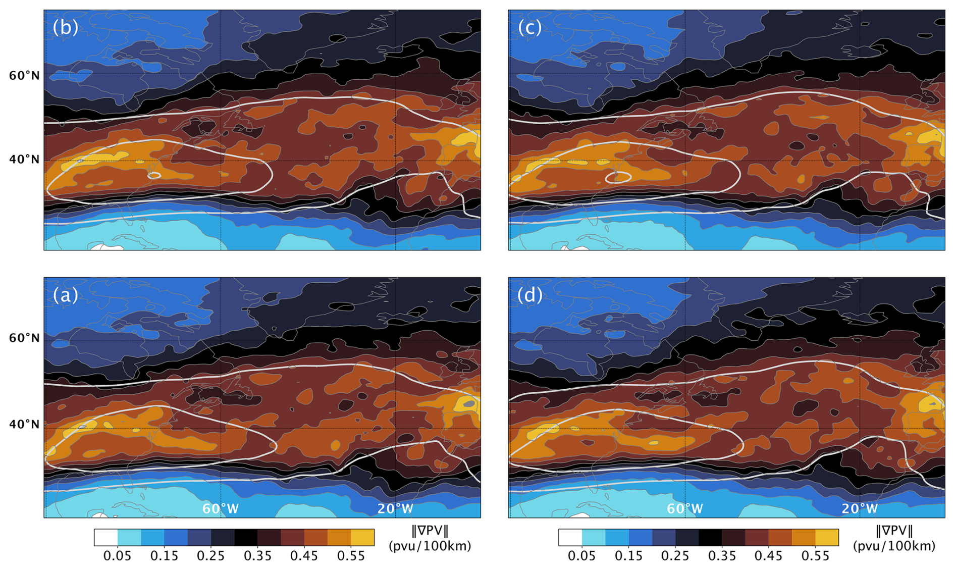
Figure F1 As in Fig. 11b but only for characteristic time steps of jet streak evolution. (a) Climatology across all time steps of maximal jet streak intensification. The PV gradient and wind speed fields on the central isentrope of the jet streak at the time of strongest intensity for each individual jet streak are considered, and the resulting 1050 PV gradient and wind speed fields are averaged to gain the climatology. (a, c, d) As in panel (b) but for the time of strongest intensity, start, and end of jet streak evolution, respectively. Note that we consider the PV and wind speed fields on the central isentrope of the jet streak at the time of strongest intensity for all four climatologies.

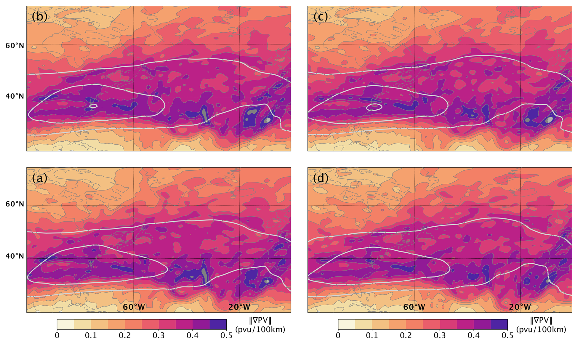
Figure F2 As in Fig. F1 but with the standard deviation of PV gradients across all jet streaks in colour and thin grey contours every 0.05 PVU (100 km)⁻¹.

Appendix G: Composite analysis of jet streak clusters

To assess how robust our results are, we present the standard deviation of jet-streak-centred PV gradients for jet streaks in C1 and C2 (Fig. G1). We find that while both clusters show substantial variability for extreme and non-extreme cases, the large-scale structure of the Rossby waves on which jet streaks reach their peak intensity is robust (anticyclonic RWB for C1 and a Rossby wave with the jet streak downstream of the ridge axis in C2).

Low-level weather systems of clusters with similar upper-level Rossby wave (RW) patterns are similar (compare panels for C1, C4, and C5 in Figs. G2 and G4 as well as C2 and C6 in Figs. G2 and G4). Figure G3 illustrates the large case-by-case variability in the locations of enhanced precipitation associated with the frontal regions of low-pressure systems within each cluster. Variability is especially large for the precipitation upstream of the jet streak centre, often related to cold-front precipitation.

The variability in upper-level flow is smaller for clusters with fewer extreme events compared to those with more extreme events, indicating more variability in large-scale flow for stronger jet streaks (compare the upper two rows to the lower four rows in Fig. G1). Note especially the low variability in the RW pattern surrounding C3 jet streaks, which is also the cluster with the weakest jet streaks that contain the fewest extreme events. Finally, WCB outflow frequencies (Fig. G6) are higher for extreme jet streak events for all clusters. The difference is most pronounced for the clusters with few extreme events. Note that for C3, only extreme cases show more than 20 % WCB outflow frequency in any region close to the jet streak centre.

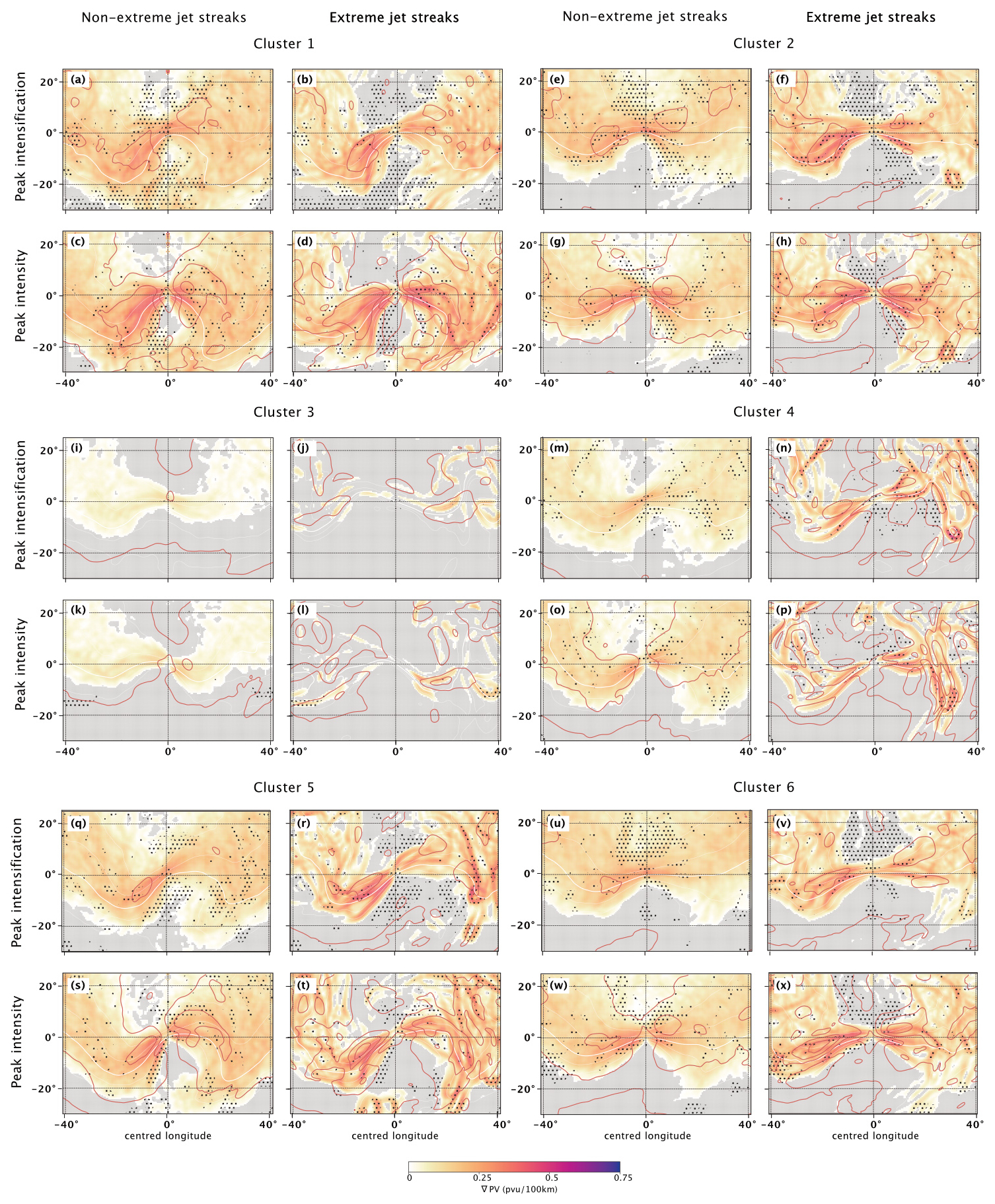
Figure G1 Jet-streak-centred composites based on bootstrapping jet streaks in C1 (a–d), C2 (g–h), C3 (i–l), C4 (m–p), C5 (q–t), and C6 (u–x). The first, third, and fifth rows show composites at the time of peak intensification, and the second, fourth, and sixth rows show the time of peak jet streak intensity. Non-extreme jet streaks are in the first and third columns and extreme jet streaks in the second and fourth columns. Colours are the standard deviation of the PV gradient (PVU (100 km)⁻¹). Dotted areas indicate where the difference between the standard deviations of the PV gradient of non-extreme and extreme jet streaks is robust. The contours are as follows: white – PV on the central isentrope; bold – 2 PVU; red – standard deviation of wind speed on the central isentrope every 5 m s⁻¹, starting at 5 m s⁻¹.

Figure G2 The colours are the mean hourly precipitation. Dotted areas indicate where the difference between the mean precipitation of non-extreme and extreme jet streaks is robust. The contours are as follows: black – mean sea level pressure every 5 hPa, starting at 970 hPa; red – PV on the central isentrope at 2 PVU. The order of panels is the same as Fig. G1.

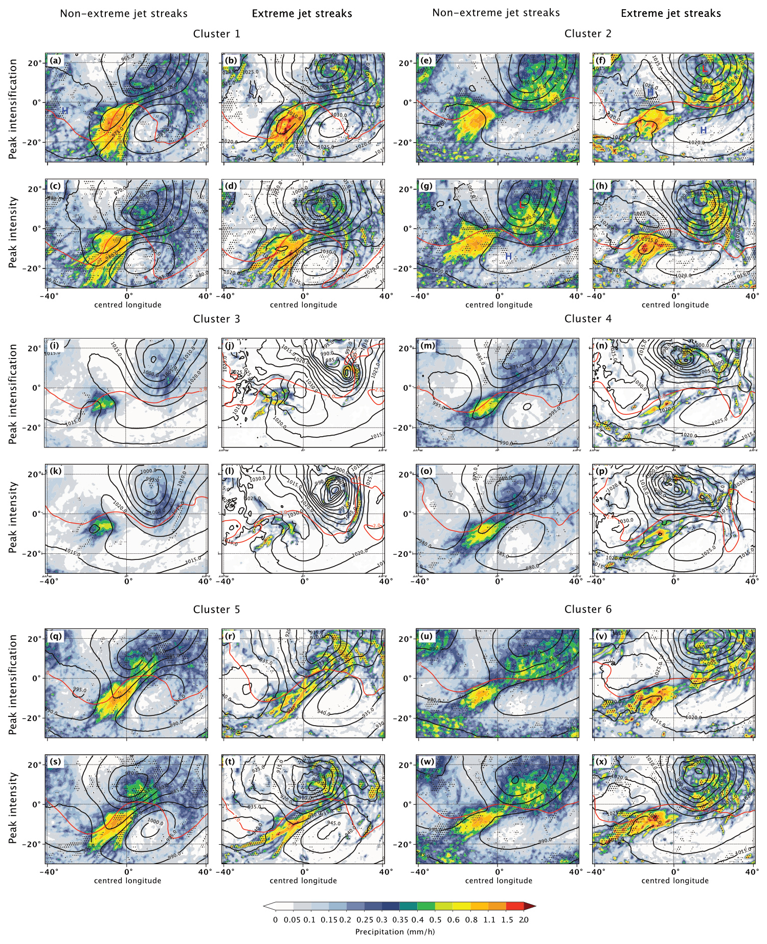
Figure G3 Colours are the standard deviation of hourly precipitation. Dotted areas indicate where the difference between the standard deviation of precipitation of non-extreme and extreme jet streaks is robust. The contours are as follows: black – mean sea level pressure every 5 hPa, starting at 970 hPa; red – PV on the central isentrope at 2 PVU. The order of panels is the same as Fig. G1.

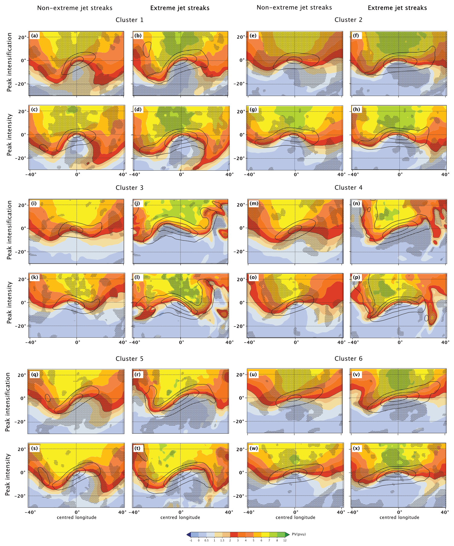
Figure G4 Colours are the mean of the PV on the central jet streak isentrope. Dotted areas indicate where the difference between the mean of the PV on the central jet streak isentrope of non-extreme and extreme jet streaks is robust. The black contours are the mean of wind speed on the central isentrope every 20 m s⁻¹, starting at 40 m s⁻¹. The order of panels is the same as Fig. G1.

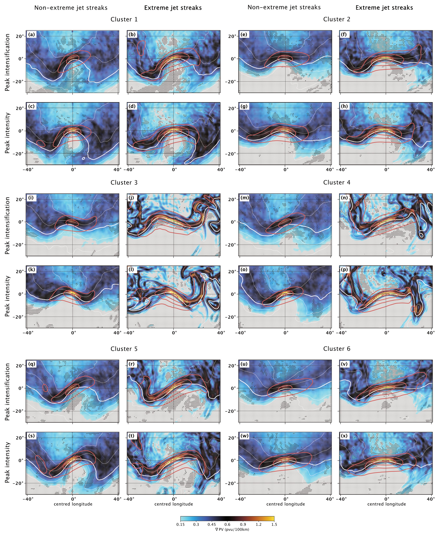
Figure G5 Colours show the PV gradient (PVU (100 km)⁻¹); values smaller than 0.15 PVU (100 km)⁻¹ are white. Dotted areas indicate where the difference between the mean of PV gradients on the central jet streak isentrope of non-extreme and extreme jet streaks is robust. The contours are as follows: white – PV on the central isentrope; bold – 2 PVU; red – wind speed on the central isentrope every 10 m s⁻¹, starting at 40 m s⁻¹. The order of panels is the same as Fig. G1.

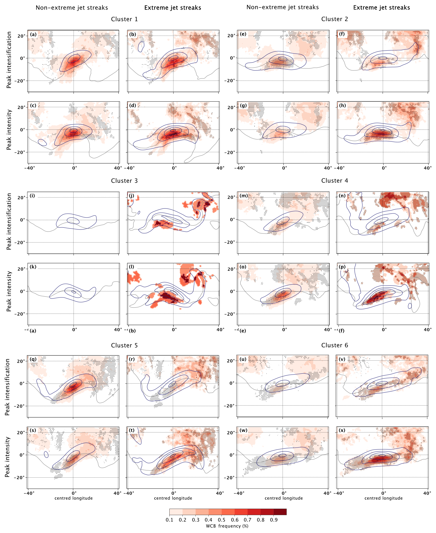
Figure G6 Colours show the WCB outflow frequency at 400 hPa. Dotted areas indicate where the difference between the WCB outflow frequency at 400 hPa of non-extreme and extreme jet streaks is robust. The contours are as follows: grey – mean PV on the central isentrope at 2 PVU; blue – mean of wind speed on the central isentrope every 20 m s⁻¹, starting at 40 m s⁻¹. The order of panels is the same as Fig. G1. Note that the lack of colours in panels (i) and (k) is not a mistake. Rather, there are no grid points with more than 10 % WCB outflow frequency at 400 hPa for non-extreme jet streaks in cluster 3.