Quantifying the spread in sudden stratospheric warming wave forcing in CMIP6

Sudden stratospheric warmings (SSWs) show a large spread across climate models in characteristics such as frequency of occurrence, seasonality and strength. This is reflective of inherent model biases. A well-known source of inter-model variability is the parameterized gravity wave forcing, as the parameterization schemes vary from model to model. This work compares the simulation of boreal SSWs in historical runs for seven high-top Climate Model Intercomparison Project Phase 6 models and in two reanalyses. The analysis is focused on the evolution of the different terms in the transformed Eulerian mean zonal mean zonal momentum equation. A large spread is found between models and with reanalyses in the mean magnitude of the resolved and parameterized wave forcing and the responses (wind deceleration and anomalous residual circulation). The results reveal that, in the stratosphere, both the wind deceleration and the strengthening of the residual circulation during SSWs correlate linearly across the models with anomalies in the resolved wave forcing. In the mesosphere, the forcing is a combination of resolved waves and, predominantly, parameterized gravity waves. Models with larger gravity wave forcing anomalies produce larger changes in the residual circulation, while models with larger resolved wave forcing anomalies produce stronger wind deceleration, which we attribute to differences in the spatial shape of resolved and parameterized wave forcing. Although the forcing–response relation across individual SSW events is similar for each model in the stratosphere, this does not hold in the mesosphere. Our results are useful for interpreting the spread in projections of the dynamical forcing of SSWs in a changing climate.

1 Introduction

Temperatures in the stratosphere have been observed to decrease in recent decades in response to increasing greenhouse gas concentrations (Randel et al., 2016; Maycock et al., 2018) and are consistently expected to continue doing so in the future (Lee et al., 2021). The dynamical response of the wintertime polar vortex in the Northern Hemisphere is, however, much more uncertain (Manzini et al., 2014; Karpechko et al., 2022). Using different scenarios of increasing CO₂ in experiments of the Climate Model Intercomparison Project Phases 5 and 6 (CMIP5 and CMIP6, respectively), Karpechko et al. (2022) concluded that half of the model spread in the future vortex mean state is related to model uncertainties. Later, Karpechko et al. (2024) attributed much of this spread in the polar vortex in CMIP6 to changes in stationary planetary wave fluxes. The projected changes in vortex variability also suffer from large uncertainty, with individual models producing robust changes of different signs in the frequency of sudden stratospheric warmings (Ayarzagüena et al., 2018, 2020).

This model spread in the representation of the vortex is present not only in future climate projections but also in simulations of the present climate, i.e., historical runs. In this context, understanding the inherent multi-model spread in the polar vortex climatology and variability is important.

It is known that the frequency of sudden stratospheric warmings (SSWs) in CMIP6 models differs from that observed in reanalyses (Ayarzagüena et al., 2020; Hall et al., 2021). This has been linked to biases in the climatological strength of the polar vortex and the upward wave activity fluxes in the lower stratosphere (Wu and Reichler, 2020). Regarding the SSW type, Hall et al. (2021) found an underestimation of split events in CMIP6, related to vortex geometry and to high filtering of wavenumber 2 and higher waves because of a stronger lower-stratospheric vortex. However, Zhao et al. (2022) found that although the spatial pattern of the polar vortex is well reproduced in CMIP6 models, it is weaker than in reanalyses, which could be linked to less accumulated wave activity flux in the stratosphere in models. The main focus of these studies has been on the simulated frequency of SSWs in models, and much less attention has been given to quantifying the wave forcing of SSWs and the response of the stratospheric circulation.

The zonal mean dynamics during the development of SSWs is the following. The strong zonal wind deceleration is driven by the anomalous Rossby wave activity flux convergence through wave breaking in the winter stratosphere (Limpasuvan et al., 2004). Using ERA5 reanalysis, Cullens and Thurairajah (2021) concluded that although SSWs' main drivers are planetary Rossby waves, gravity waves also contribute to their occurrence. Moreover, for the austral polar vortex breakdown, both resolved and parameterized gravity waves in ERA5 were found to be important (Gupta et al., 2021). Wave breaking in the extratropical stratosphere not only decelerates the vortex but also induces a strengthened poleward residual circulation (e.g., de la Cámara et al., 2018). This motion causes downwelling and adiabatic heating over the polar stratosphere. Weakened westerlies allow more eastward gravity waves to propagate up to the mesosphere. Consequently, the mesosphere experiences anomalous positive gravity wave forcing (more eastward gravity waves), decelerating the mesospheric residual circulation (Liu and Roble, 2002), cooling it over the pole and sinking the stratopause down to lower levels (Von Zahn et al., 1998; Limpasuvan et al., 2012). Once the zonal wind reversal has taken place, stationary planetary waves can not propagate upward, and the wave forcing rapidly decreases, allowing westerly winds to recover at upper levels, while they stay weak in the lower stratosphere due to the longer radiative damping timescales (Newman and Rosenfield, 1997).

The relatively broad spatial resolution of climate models limits the wavelengths that can be explicitly resolved, and a large part of the gravity wave spectrum needs to be parameterized, even in high-resolution models. The parameterization schemes vary in each model, giving rise to a wide variety of gravity wave representation and interactions with the resolved flow, which introduces a source of discrepancy among models.

In this work we analyze the model spread in resolved and parameterized wave forcing during SSWs in seven CMIP6 models and two reanalyses. We study, for the SSWs in each model, how the circulation responses change for different forcings and how this is reproduced in models. How much of the wave activity flux convergence is translated into advection of the residual circulation and how much into wind deceleration across models? How different are the contributions of resolved and parameterized waves? The answer to these questions in historical simulations, comparable with reanalyses, will be valuable for understanding future projections of a changing climate.

The article is organized as follows: dataset characteristics and methods are described in Sects. 2 and 3. An analysis on the spread in the representation of sudden stratospheric warmings in the datasets is presented in Sect. 4, first focused on the mean representation of SSWs and then on their variability. Finally, the conclusions are summarized in Sect. 5.

2 Data

In the present work we use seven high-top models in CMIP6 with historical (all-forcing simulation of the recent past) experiments, from 1850 to 2014 (to 2009 in some models), and one or three runs, depending on the model. They are listed in Table 1 with information about their resolution, model top and parameterization schemes on orographic gravity waves (OGWs) and non-orographic gravity waves (NOGWs). These models provide the output of the contributions to the momentum balance in the TEM formulation as described in Gerber and Manzini (2016). For HadGEM3-GC31-LL and UKESM1-0-LL, tendencies due to meridional and vertical momentum advection terms are not available and have been calculated from other outputs, possibly leading to numerical errors. Both models are developed by the Met Office, so they share most of their components, e.g., gravity wave parameterization scheme. Moreover, MIROC6 and MRI-ESM2-0 share an NOGW parameterization. We highlight that CESM2-WACCM includes NOGW sources by convection and frontal systems and IPSL-CM6A-LR also includes NOGWs due to precipitation (Lott and Guez, 2013) and from frontal systems via a spontaneous adjustment mechanism (de la Cámara and Lott, 2015).

Scinocca and McFarlane (2000)Richter et al. (2010)Beres et al. (2005)Garner (2005)Alexander and Dunkerton (1999)Vosper (2015)Warner and McIntyre (2001)Lott (1999)Lott and Guez (2013)de la Cámara and Lott (2015)McFarlane (1987)Hines (1997)Iwasaki et al. (1989)Hines (1997)Vosper (2015)Warner and McIntyre (2001)

Table 1 CMIP6 models with historical experiments used and their characteristics. In the Variant_id column, the brackets show the different runs used. The historical experiment covers 1850 to 2014, except for GFDL-ESM4 and IPSL-CM6A-LR, which only extend to 2009.

Additionally, we use reanalysis data for comparison. We use the transformed Eulerian mean dataset from the MERRA-2 and ERA5 reanalyses, as presented in Serva et al. (2024). The products are obtained by computation from 6-hourly data following Gerber and Manzini (2016). For MERRA-2, 72 native vertical levels to 1 Pa and a native spatial resolution of 0.5° × 0.625° (Gelaro et al., 2017) are used for the computation, covering 1980 to 2021. For ERA5, 137 native vertical levels to 1 Pa and a 0.5° × 0.5°° grid are used, while a native spatial grid of 0.25° × 0.25° is used (Hersbach et al., 2020), covering 1959 to 2021. In both datasets the contribution of gravity wave “drag” (GWD) is provided as a single term, not separated into OGWs and NOGWs as in the models. Therefore, in this work we analyze OGWs and NOGWs together as a GWD. In MERRA-2, GWD is only available up to 0.1 hPa.

3 Methods

We identify boreal SSWs in every climate model and the two reanalyses. The detection of SSWs is based on the criterion proposed by Charlton and Polvani (2007). The onset day of the event (lag 0) is set when the zonal mean zonal wind at 60° N and 10 hPa crosses zero, provided no other event has been detected in the previous 20 d. The generation of SSWs by different models varies in total frequency and the month of the year (Ayarzagüena et al., 2020; Wu and Reichler, 2020; Hall et al., 2021). This can be due to different vertical resolutions and lid heights (Wu and Reichler, 2020) and should be taken into account when comparing the models. Figure 1 shows the distribution of SSW occurrence through the extended winter in each model of the present study, with the relative frequency of detected SSWs over the number of years in brackets. Only the common period with ERA5 has been taken, i.e., from 1959 to 2009 (1980 to 2009 for MERRA-2). Except for IPSL-CM6A-LR and GFDL-ESM4, all models generate fewer SSWs than observed with both reanalyses. However, IPSL-CM6A-LR is the only one statistically significant at 95 % confidence, using a parametric test as in Gu et al. (2008). Reanalyses also differ slightly from each other as the datasets do not fully match in time, but they agree over their common period (1980–2021; see Serva et al., 2024). We can also see that there is no agreement in the monthly distribution between models and reanalyses, as shown in Ayarzagüena et al. (2020). While January and February are the months with the highest frequency of SSWs in the reanalyses, in the models we find a more uniform distribution throughout the winter, with some biases towards late winter. Furthermore, some results are tested with the approach of sudden stratospheric decelerations (SSDs), as done in Birner and Albers (2017). Differently from the absolute threshold for the event detection of Charlton and Polvani (2007), this criterion uses a relative threshold of 2 standard deviations in wind deceleration, whose value is model dependent. In Fig. S18 of the Supplement, it can be seen that there are also discrepancies between models and reanalyses in the frequency and seasonality of SSD occurrence.

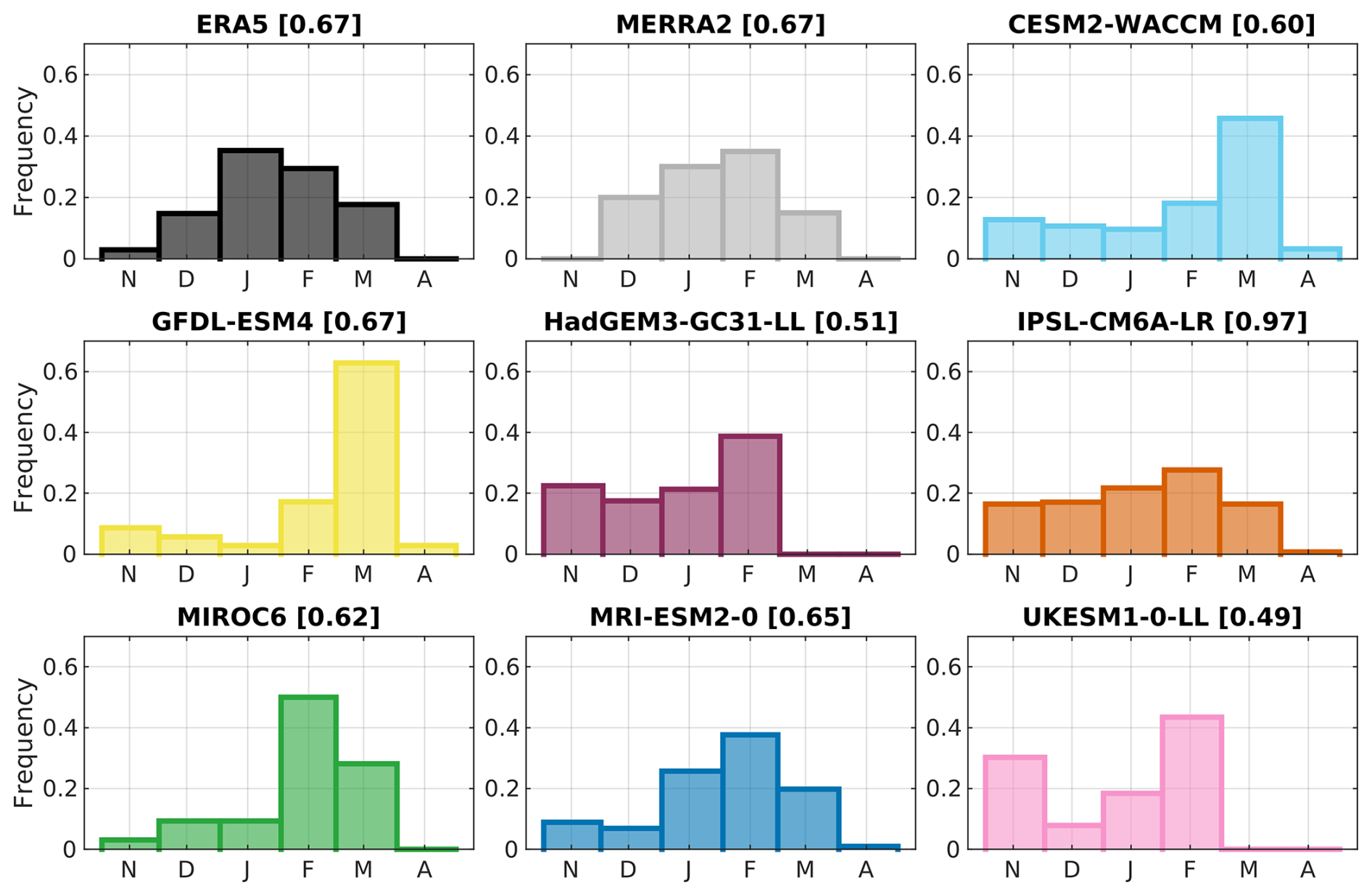
Figure 1 Monthly distribution of SSW frequency relative to the total number of events in each model and reanalyses on the common period (1959–2009). Brackets show the SSW total frequency (number of events per year).

In this work we focus on analyzing the terms of the momentum balance equation in the transformed Eulerian mean (TEM) formulation. Following Andrews et al. (1987), the meridional residual circulation in the TEM framework has a northward and a vertical component $({\stackrel{\mathrm{‾}}{v}}^{\ast },{\stackrel{\mathrm{‾}}{w}}^{\ast })$. The TEM zonal momentum equation is then written as follows:

$$\begin{array}{}\text{(1)}& {\stackrel{\mathrm{‾}}{u}}_t+\mathit{\{}-{\stackrel{\mathrm{‾}}{v}}^{\ast }\widehat{f}+{\stackrel{\mathrm{‾}}{w}}^{\ast }{\stackrel{\mathrm{‾}}{u}}_z\mathit{\}}=\left\{{\displaystyle \frac{e^{\frac{z}{H}}}{a\cos \mathit{\varphi }}}\mathrm{\nabla }\cdot \mathit{F}+{\stackrel{\mathrm{‾}}{\mathit{\chi }}}_{\mathrm{param}}\right\}+\mathit{\epsilon },\end{array}$$

where $\widehat{f}=f-\frac{\mathrm{1}}{a\cos \mathit{\varphi }}{\left(\stackrel{\mathrm{‾}}{u}\cos \mathit{\varphi }\right)}_{\mathit{\varphi }}$ in which f is the Coriolis parameter, F is the Eliassen–Palm flux, ${\stackrel{\mathrm{‾}}{\mathit{\chi }}}_{\mathrm{param}}$ is the parameterized physics forcing and ε is the residual computed by the imbalance between both sides of the equation.

The terms in Eq. (1) represent (from left to right) the following. On the left-hand side is the temporal derivative of the zonal mean zonal wind (Ut) and in braces the meridional and vertical advection of absolute angular momentum by the residual circulation (ADV). On the right-hand side the term in braces provides the total eddy-induced zonal mean force. This includes a contribution from resolved waves (EPD), basically from planetary waves, as the divergence of the Eliassen–Palm flux, and a contribution from parameterized waves (GWD), basically gravity waves.

The residual mean velocities ${\stackrel{\mathrm{‾}}{v}}^{\ast }$ and ${\stackrel{\mathrm{‾}}{w}}^{\ast }$ (defined in Andrews et al., 1987) may be expressed in terms of a stream function Ψ, where Ψ can be calculated as

$$\begin{array}{}\text{(2)}& \mathrm{\Psi }(\mathit{\varphi },z)={\mathit{\rho }}_{\mathrm{0}}\cos \left(\mathit{\varphi }\right)\underset{z}{\overset{\mathrm{\infty }}{\int }}{\stackrel{\mathrm{‾}}{v}}^{\ast }{e}^{-\frac{z^{\prime }}{H}}\mathrm{d}{z}^{\prime }.\end{array}$$

Finally, anomalies are calculated as the departure from the smoothed daily evolving annual cycle of each model, which is in turn defined based on a running 30-year mean. The statistical significance of the anomalies is assessed applying a two-tailed Student's t test.

4 Results

4.1 SSW evolution in models and reanalyses

Before comparing the performance of different models, Fig. 2 shows the composite evolution of the anomalies of the different terms in Eq. (1) during SSWs in ERA5 and displays well-known features of the life cycle of SSWs. There is a strong deceleration of the zonal mean winds during the 7 d before the central date (Fig. 2a), followed by an acceleration that is stronger in the upper levels than in the lower stratosphere, where the negative wind anomalies persist for at least 1 month. This contrasting evolution of the winds at different levels in the aftermath of SSWs is mainly the result of the faster radiative timescales at upper levels (Hitchcock et al., 2013b).

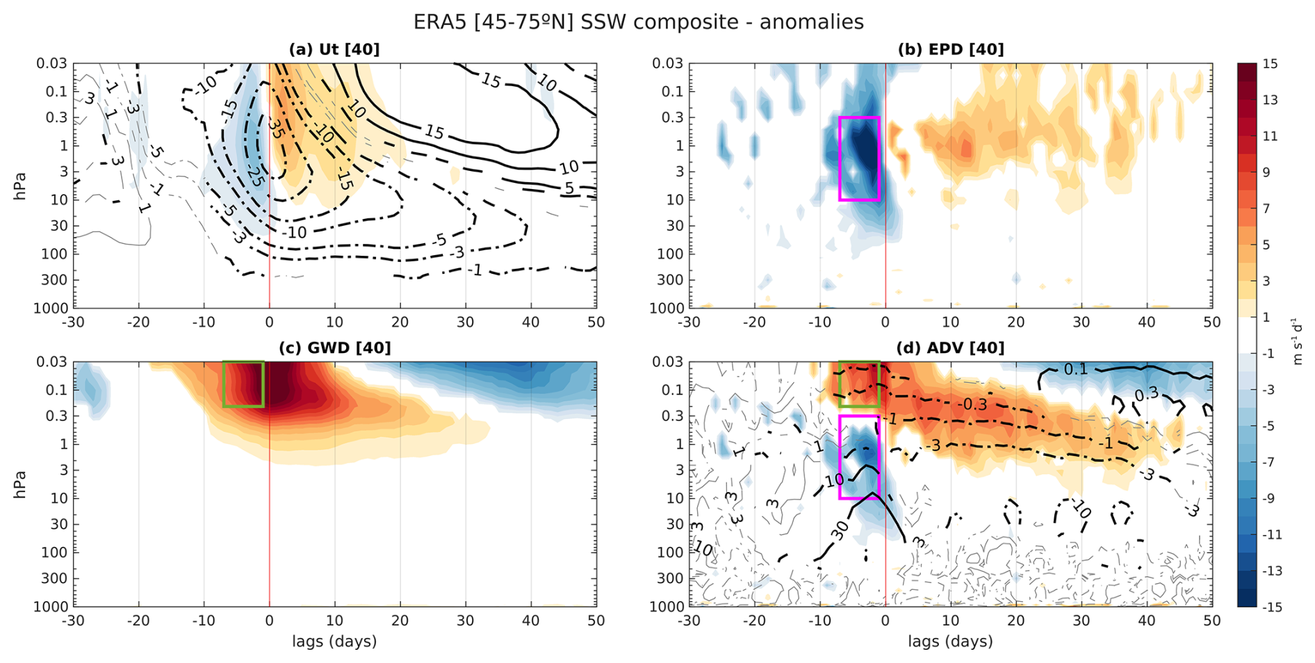
Figure 2 Lag–height SSW composite evolution of zonal mean (45–75° N) area-averaged anomalies of (a) the tendency of the zonal wind, (b) planetary Rossby wave drag, (c) gravity wave drag and (d) the Coriolis torque of the residual circulation in shading for the ERA5 reanalysis. The contours show anomalies of zonal wind in panel (a) and the mass stream function in panel (d). Units are m s⁻¹ d⁻¹ for shading and m s⁻¹ and kg m⁻¹ s⁻¹ in panels (a) and (d) for contours, respectively. The shaded colors and thick black contours indicate values significant at 95 % confidence with a two-tailed t test. The number of SSWs in the composite is shown in brackets. The pink (10–0.3 hPa (45–75° N), −7 to −1 lags) and green (0.2–0.03 hPa (45–75° N), −7 to −1 lags) boxes are used to average fields in subsequent analyses.

The initial wind deceleration is driven by the negative resolved wave forcing anomalies with a peak at around 1 hPa and lag −3 (Fig. 2b). This deceleration ceases abruptly after lag 0, and there even appear weak positive anomalies in the upper stratosphere and lower mesosphere during the following 50 d. The parameterized forcing induces anomalous acceleration mainly from lags −10 to 20 at mesospheric levels (above 1 hPa, Fig. 2c), likely as a result of reduced eastward GW filtering by the weak winds in the stratosphere below. Both the build-up and the disappearance of these anomalies are more gradual than those of the resolved forcing. The positive anomalies at positive lags have previously been suggested to contribute to the upper-level westerly wind recovery in the aftermath of SSWs (Hitchcock et al., 2013a).

The evolution of the residual mean momentum advection is determined by the combination of the resolved and parameterized forcings (Fig. 2d). At negative lags during the wind deceleration, there are negative anomalies in the stratosphere below 1 hPa (forced by the resolved forcing) and positive anomalies above (forced by the parameterized forcing); at positive lags the evolution resembles that of the parameterized forcing.

Similar figures to Fig. 2 but for the climate models and MERRA-2 can be found in the Supplement (Figs. S1–S8), with qualitatively similar evolutions. To facilitate the inter-model comparison, we show in Fig. 3 the evolution of EPD (solid) and GWD (dashed) in the left column and Ut (solid) and ADV (dashed) in the right column at some selected layers for the SSW composite mean anomalies. Each line represents the evolution of a different model mean.

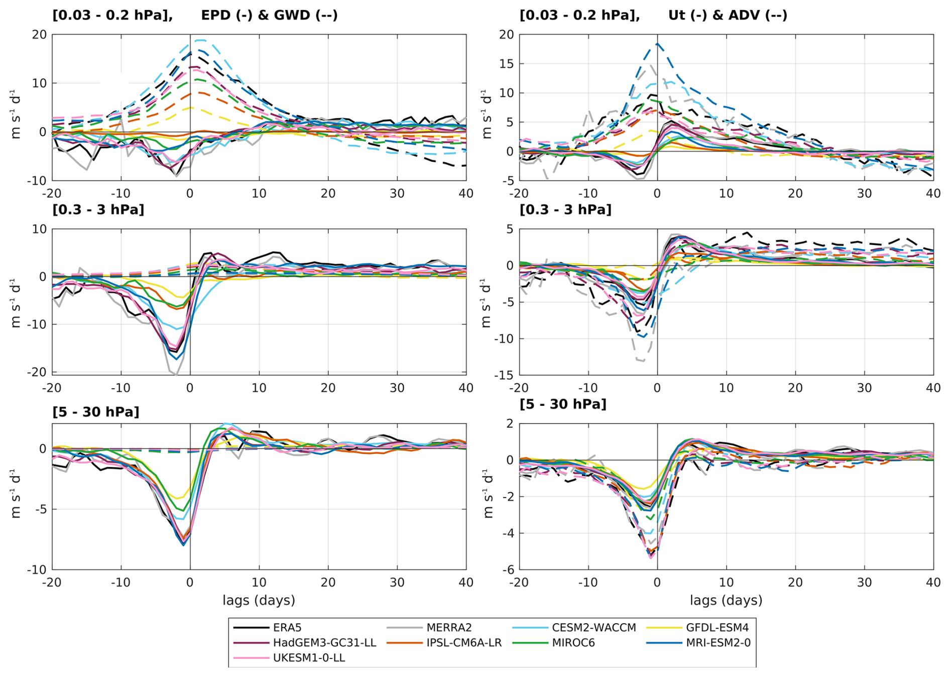
Figure 3 Evolution of EPD (solid) and GWD (dashed) in the left column and Ut (solid) and ADV (dashed) in the right column for the SSW composite mean. Each colored line represents a CMIP6 model or a reanalysis. The rows show the average at different pressure layers. Variables are zonal means and area averaged (45–75° N).

We can see that there is agreement on the sign of the evolving anomalies among the models but with large inter-model spread, especially in the mesosphere. Different sponge layer thicknesses and biases in the climatologies (Fig. 4) are likely to play a role in these model differences.

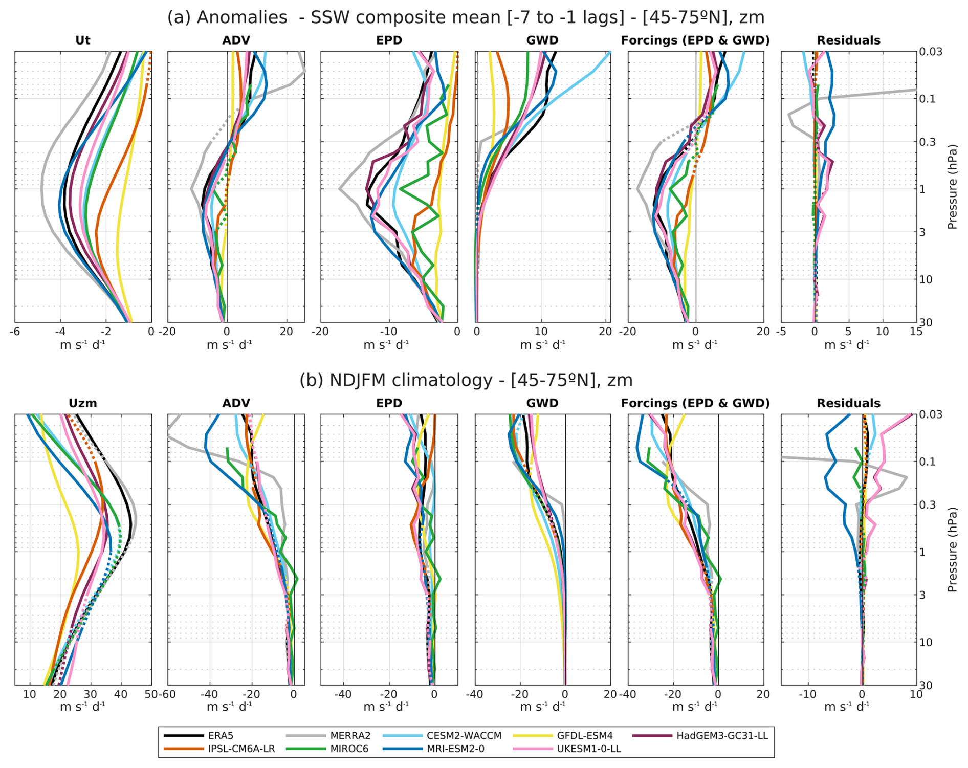
Figure 4 Vertical profiles of (a) SSW composite mean anomalies and (b) extended winter climatology of the models and reanalyses, (45–75° N) area averaged. Each colored line represents a CMIP6 model or a reanalysis. The panels (from left to right) show the following variables: zonal mean zonal wind tendency (a) and climatology (b), advection by the residual circulation and Coriolis effect, tendency of eastward wind due to Eliassen–Palm flux divergence, parameterized non-orographic and orographic gravity wave drag, the total wave forcing (sum of the previous two terms), and the residual errors in Eq. (1). The dotted lines indicate non-significance (a) at 0.95 with a t test in the composite mean and (b) in differences from ERA5 reanalysis.

The spread in the mesospheric GWD anomalies around the onset date is comparable to the multi-model mean, with values across models from 5 to 19 m s⁻¹ d⁻¹ (see panels of 0.03–0.2 hPa). ERA5 reanalysis and the CESM2-WACCM and MRI-ESM2-0 models produce the largest GWD anomalies in the mesosphere, whereas GFDL-ESM4 and IPSL-CM6A-LR have the weakest.

The largest anomalies and spread in EPD are found in the upper stratosphere–lower mesosphere (see panels of 0.3–3 hPa) around 1 week prior to the onset date. Again, a wide range of values can be found across models, varying from −5 to −20 m s⁻¹ d⁻¹. In the mesosphere and stratosphere the anomalies are weaker, with less spread in the stratosphere.

The responses also show large spread across models. Prior to the onset date in the mesosphere, the anomalies and forcings have opposite signs. Wind acceleration and EPD anomalies are negative at all levels, while ADV is positive in the mesosphere, similar to GWD, and negative below.

We argue that in the stratosphere EPD drives both responses as GWD is relatively low. However, in the mesosphere positive ADV is driven by positive GWD and negative Ut by negative EPD anomalies. We come back to this point below.

4.2 Model mean spread during the SSW development stage

A burst of EPD and strong wind deceleration occurs approximately 1 week before the onset date (Figs. 2 and 3). We focus on this period for the subsequent analysis, referring to it as the development stage. To characterize this stage, we selected −7 to −1 lags, as marked by the pink and green boxes in Fig. 2. The sensitivity to the choice of these lags has been tested for some relevant results, as explained later. In this section we compare the SSW composite mean and quantify the biases across models during the development stage.

During the development stage the main contribution to the total forcing (EPD + GWD) anomalies in the stratosphere is EPD, with much weaker GWD anomalies (Fig. 4a). The spread through the models is notable, with the largest differences around 1 hPa. However, in the mesosphere the anomalous wave forcing is dominated by the reduction in the climatological westward GWD (Fig. 4b), producing positive anomalies. The spread through the models is large in stratospheric EPD and mesospheric GWD anomalies. Below 30 hPa the values converge. This also happens in the climatology (Fig. 4b), with the spread growing with height.

Even though the total forcing anomalies reverse from negative in the stratosphere to positive in the mesosphere, the wind is decelerated at all levels, with maximum values occurring between 1 and 5 hPa depending on the model. In the mesosphere all models underestimate Ut and the climatological zonal mean zonal wind compared to the reanalyses. In contrast with Ut, ADV anomalies do reverse like the total forcing. While this change of sign occurs in all models, models differ on the height at which this happens.

One should note that the balance is not fully closed as there are still some residuals, even in the climatology. The MERRA-2 residual in particular stands out. This reanalysis has strong wind deceleration and anomalous residual advection in the mesosphere but a comparable EPD to the rest of the models. This can only be compatible with very strong anomalous GWD, but as this field is not provided above 0.1 hPa, the residual is necessarily large. Similar outstanding residuals of Eq. (1) in MERRA-2 are found in the tropical mesosphere by Ern et al. (2021).

To quantify the spread across models, we distinguish between the stratosphere and the mesosphere based on the sign change. Taking into account that above 0.2 hPa all models produce positive ADV and forcing anomalies, we characterize the stratospheric and mesospheric anomalies in the following, vertically averaging over the pink and green boxes in Fig. 2, i.e., from 10 to 0.3 hPa and from 0.2 to 0.03 hPa, respectively. For MIROC6 the mesospheric averages are computed from 0.2 to 0.07 hPa, as data above that level were not available for this model.

Using “strat” and “meso” to refer to the regions defined as stratosphere and mesosphere, Fig. 5 shows various relations between the variables in Fig. 4a vertically integrated as indicated above.

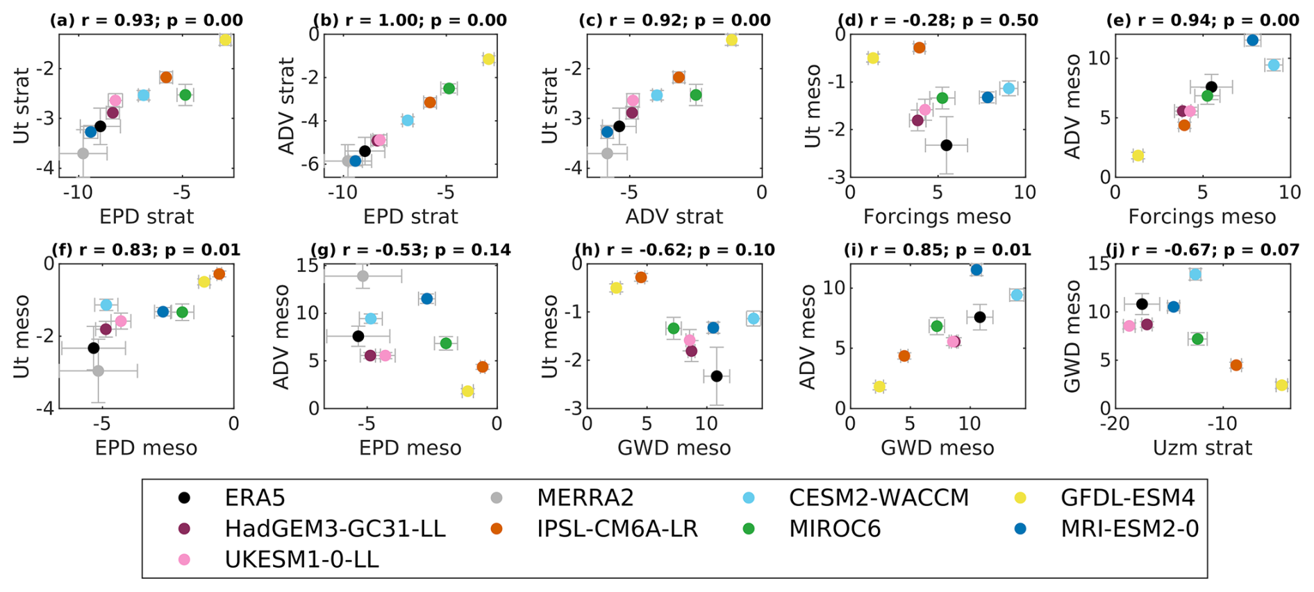
Figure 5 Scatter plots for the SSW composite mean of area-averaged fields at 45–75° N and −7 to −1 lags. Variables are area averaged from 10 to 0.3 hPa (“strat”) and from 0.2 to 0.03 hPa^* (“meso”). Units are m s⁻¹ d⁻¹. The error bars show the standard error of the mean, taking into account all SSWs for each model, and the panel titles indicate the linear correlation coefficient (r) and p value. ^* From 0.2 to 0.07 hPa for MIROC6.

As expected from Eq. (1), EPD in the stratosphere is linearly correlated with Ut and ADV (Fig. 5a, b). In both cases the correlation increases slightly when GWD is also included (not shown). The wind deceleration is also highly correlated with the advection in the stratosphere (Fig. 5c).

In the mesosphere, the total forcing is a combination of EPD and GWD. We can see that the total forcing correlates well with ADV but not with Ut (Fig. 5d, e). When looking at the forcings separately, we find that GWD is only correlated with ADV, and EPD is only correlated with Ut (Fig. 5f, i). The latter is consistent with the findings in Fig. 3 (top) that the smaller EPD forcing plays a more important role than GWD in driving the zonal wind variability at mesospheric levels. To assess robustness, we repeated the analysis with composites of SSDs (Fig. S19), obtaining the same relations but with a somewhat larger scatter.

These results suggest that the GWD forcing is in quasi-steady balance with the residual advection, driving only a small part of the zonal wind variability. Because the total forcing is dominated by GWD but the zonal wind variability is driven primarily by EPD, there is no significant correlation between the total forcing and the wind tendency (Fig. 5d) as noted before.

The different characteristics of the responses to GWD and EPD may reflect differences in the spatial structure of the forcings. The aspect ratio of a forcing determines how much of the response translates into zonal wind deceleration and how much into residual advection (Nakamura, 2024; Pfeffer, 1987). As shown in Eqs. (A1) and (A2) in Appendix A, Ut is forced by the second meridional derivative of the wave forcing, while ADV is forced by the second vertical derivative. Thus, shallow forcings will produce a stronger ADV response, and deep forcings will produce a stronger Ut response. As shown in Fig. 2, the planetary forcing EPD is deep, as it follows the polar vortex across the stratosphere and mesosphere, while the parameterized forcing GWD is shallow and concentrated at mesospheric levels (for more details, see latitude–height cross sections in the Supplement, Figs. S9–S17). This is consistent with their corresponding responses.

Another factor that may play a role in the different responses to EPD and GWD is their different timescales. As is also apparent in Fig. 2 (and clearer in non-composited time series, not shown), GWD evolves more slowly than EPD, so we expect the response to GWD to vary in longer timescales than the response to EPD. We speculate that the different timescale of the two forcings may be due to the filtering effect of the stratospheric mean flow, essentially a time integration of the stratospheric EPD anomalies.

Finally, Fig. 6 shows that part of the spread across models can be explained by the inherent spread in their climatologies (Kim et al., 2017). Models with large climatological EPD values tend to also display large anomalies in the SSW composite. The same can be seen for the wind deceleration and the climatological zonal mean zonal wind. Interestingly, IPSL-CM6A-LR produces large EPD climatological values, while it has the weakest climatological zonal wind. The opposite occurs for MIROC6. In contrast, GFDL-ESM4 has both weak EPD and weak Uzm climatologies.

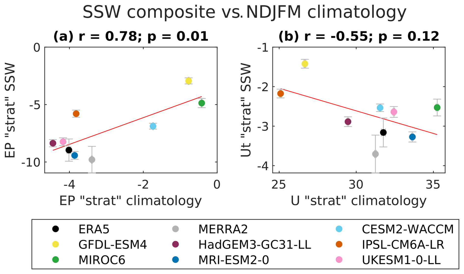
Figure 6 Scatter plots of SSW composite mean anomalies and climatology of EPD (a) and Ut (b) in the extratropical stratosphere (10 to 0.3 hPa and 45 to 75° N).

4.3 Inter-event variability in models during the SSW development stage

After having studied the biases between models in the mean SSW representation, we now analyze the event-to-event variability in the forcings and circulation responses during the development stage of SSWs. We quantify how much of the resolved and parameterized wave deposition of momentum is translated into advection by the residual circulation and wind deceleration for every SSW simulated in the datasets.

Starting with the stratosphere, we quantify the relationship between the main forcing during the development stage, EPD, and the two responses, ADV and Ut. Since GWD is negligible in this region, it is not taken into account. As expected from Eq. (1), the relation between EPD and the sum of Ut and ADV anomalies is completely linear (not shown). When separating the responses we also find linearity between EPD and both ADV and Ut, especially with ADV. This is shown in Fig. 7a, which also provides the linear correlation coefficient and the least-squares fit for both responses: ADV ∼ m1 EPD + c1; Ut ∼ m2 EPD + c2.

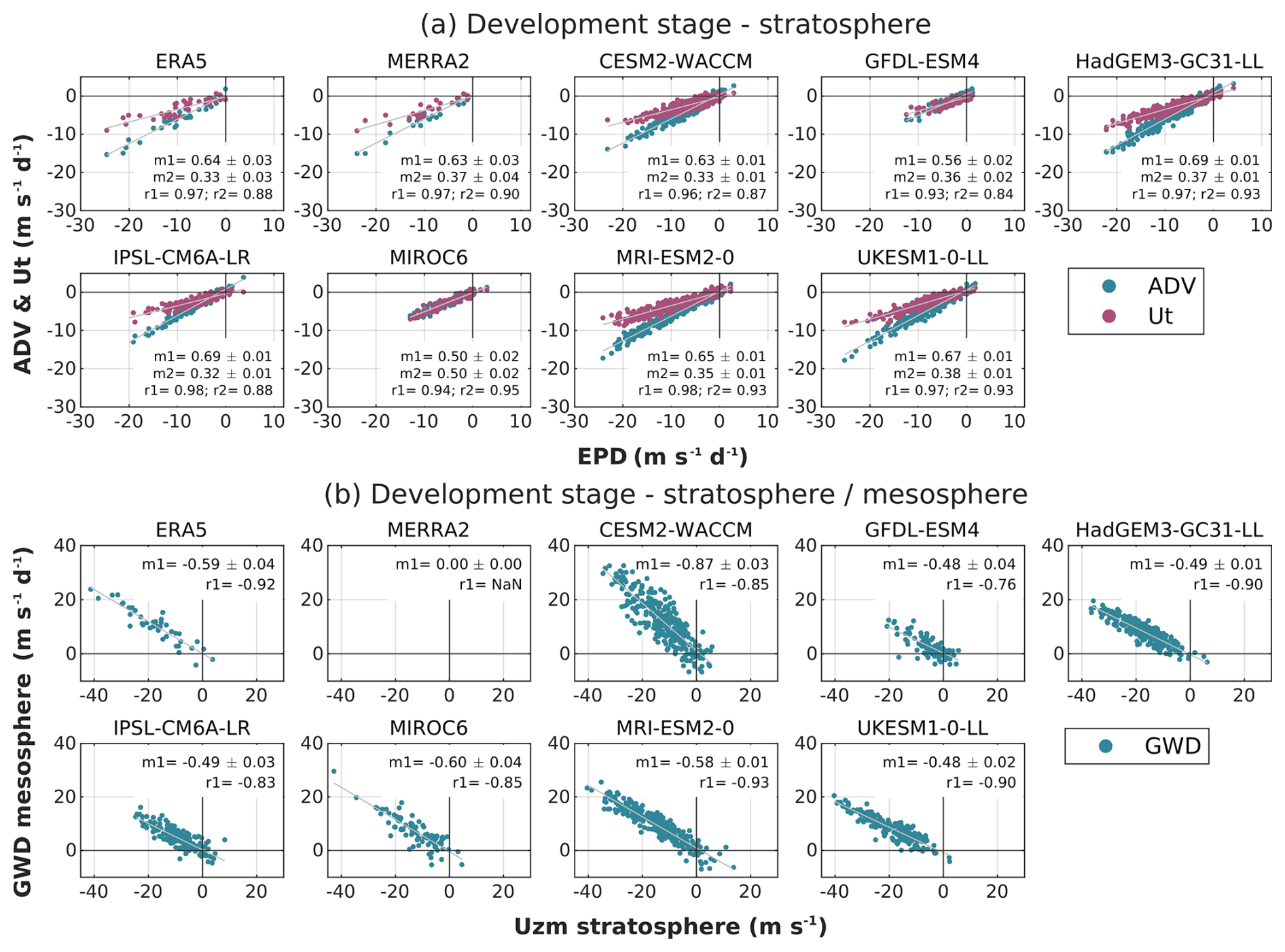
Figure 7 Scatter plots of the same variables as in Fig. 5 for all SSWs in the models and reanalyses. (a) EPD versus ADV and Ut in the stratosphere and (b) zonal mean zonal wind in the stratosphere versus GWD in the mesosphere. Stratospheric variables are averaged from 10 to 0.3 hPa and mesospheric variables from 0.2 to 0.03 hPa, and both are area averaged from 45–75° N. Linear fits y ∼ mx+c are also shown (gray lines), and the corresponding slopes (m1/m2 for ADV/Ut in panel a and m1 for GWD in panel b) are indicated in the text. The corresponding linear correlation coefficients, r1 and r2, are also provided.

We find large correlation coefficients with values between 0.93 and 0.98 for ADV and 0.84 and 0.95 for Ut. The linear fit reveals that in both cases almost all models have similar slopes. This suggests that the dynamical relationship between both variables is similar for all models, although there is some spread in the composite mean. Almost all models agree that approximately $\mathrm{2}/\mathrm{3}$ of the EPD forcing is translated into ADV and $\mathrm{1}/\mathrm{3}$ into wind deceleration, irrespective of the magnitude of the forcing. The exception is MIROC6, for which the response is translated equally into ADV and the deceleration of the wind. We can see that MIROC6 is also an outlier in Fig. 5a. GFDL-ESM4 also differs for the ADV relation. This $\mathrm{2}/\mathrm{3}$ to $\mathrm{1}/\mathrm{3}$ ratio is roughly consistent with the findings of Nakamura et al. (2020) that about 60 % of the wave forcing is balanced by residual advection, and 40 % is used to decelerate the zonal wind for ERA-Interim and MERRA-2 SSWs.

Moreover, we can see that for all models the slopes in both regressions are complementary so that they approximately add up to 1. A sensitivity test (Fig. S20) shows that these slopes are robust when changing the lags used to average.

In contrast, we find that EPD is not linearly correlated with the wind anomaly (not shown). It is also interesting that no events with positive EPD anomalies are observed in the reanalyses, while they can be produced by the models.

In the mesosphere (Fig. 8) the behavior is a bit more complex since gravity waves also play a role, and the residuals are larger. However, the residuals do not seem to bias the relations as the correlation between the total forcings and both responses together is still close to 1 (not shown). The only exception is MRI-ESM2-0, which has the largest residuals (Fig. 4a). Before discussing the relative impact of EPD and GWD, we first analyze how the response to the total forcing (EPD+GWD) is split between ADV and Ut. As in the previous section, we consider in Fig. 8 averages from −7 to −1 lags, 0.2 to 0.03 hPa and 45–75° N. For MIROC6 the vertical average only extends up to 0.07 hPa, as data for some variables were not available at higher levels for this model. Figure 8a shows that there is again a good correlation between the total forcing and ADV, though the scatter is larger than in the stratosphere. This may be due to higher inter-event variability in the partition of the response between ADV and Ut.

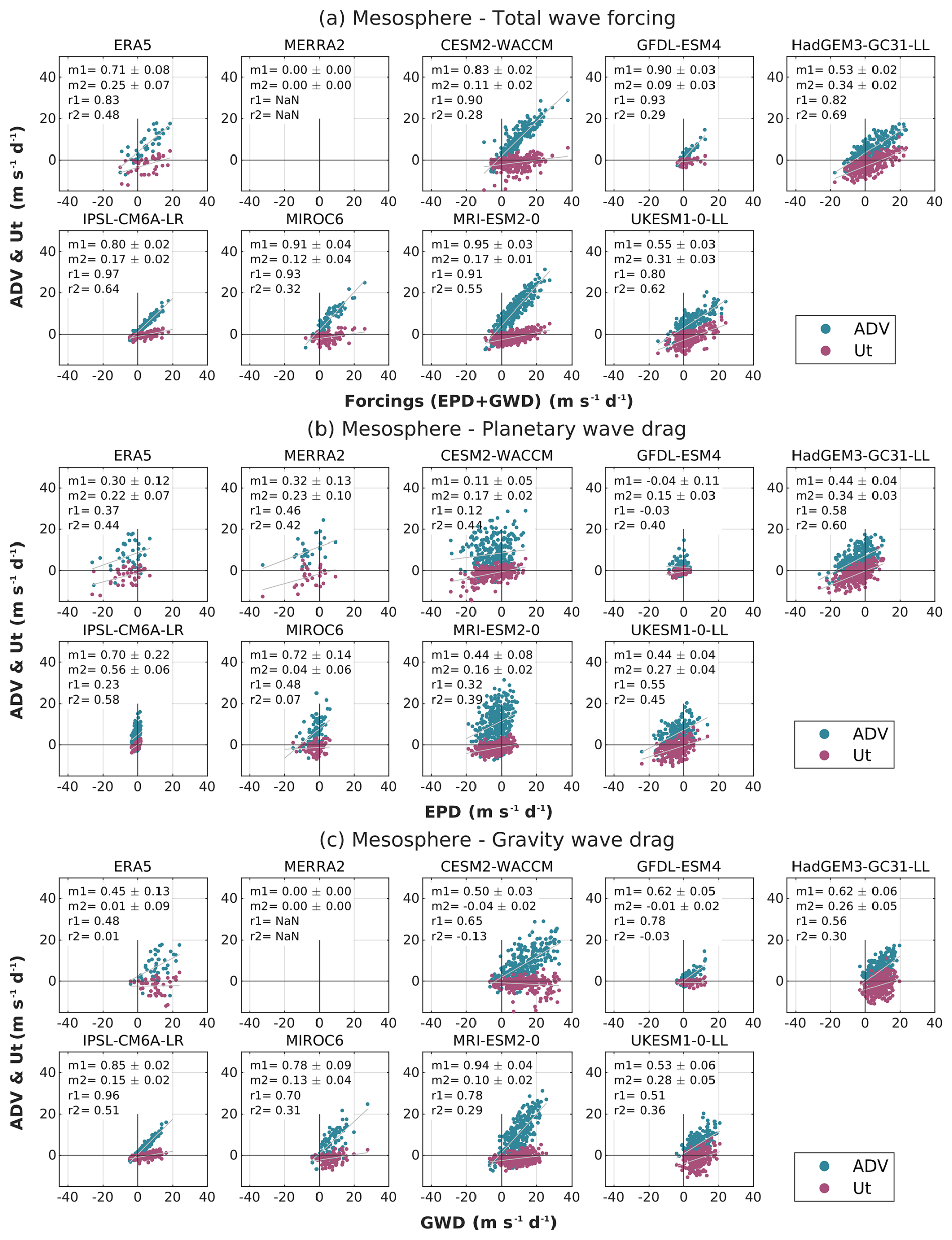
Figure 8 As in Fig. 7 but relating (a) the total wave forcing (EPD + GWD), (b) EPD and (c) GWD both with ADV and Ut in the mesosphere (0.2 to 0.03 hPa^* and 45 to 75° N). ^* From 0.2 to 0.07 hPa in MIROC6 due to data unavailability.

We also note that the slope of the fit can vary substantially across models. The fact that all slopes exceed 0.5 implies that ADV dominates the response to the forcing. However, this happens to different degrees in different models. In some models (CESM2-WACCM, GFDL-ESM4, MIROC6 and MRI-ESM2.0) the slope is close to 1, suggesting that zonal wind variability plays little role in the response to the forcing for these models. Flatter slopes 𝒪(0.7) are found for ERA5 and IPSL-CM6A-LR, while the two Met Office models have the smallest slopes, 𝒪(0.6). We also analyzed the sensitivity of this linear fitting to the lags used for averaging (see Fig. S21). The slope for the Ut (ADV) fitting decreases (increases) slightly when extending the time windows at negative lags. This is consistent with the transient nature of Ut: for long time averages Ut should vanish, and the full forcing should be balanced by ADV. As shown in Fig. 8a, in general the linear correlation between the forcing and Ut is better (and the slope of the fit is larger) for the models with a smaller ADV slope, such as UKESM1-0LL and HadGEM3-GC31-LL. In contrast, there is only noise in the scatter plot between the forcing and Ut for models such as CESM2-WACCM and GFDL-ESM4, for which ADV alone balances the response to the forcing.

We next investigate the relative role of GWD and EPD in producing these responses (Fig. 8b and c). Consistent with the composite results, EPD is strongly biased to negative values and GWD to positive values, though there is significant inter-event variability (including values of the opposite sign) in most models. We recall that in the composite mean, GWD is the dominant forcing. Moreover, there is no linearity in the GWD versus EPD relation (not shown), pointing out that there is not a fixed balance between them. Most models produce a linear relation between GWD and ADV (Fig. 8c), although the slopes of the fit vary substantially across models. In contrast, there is no linearity with Ut.

As regards EPD, we showed before that in the composite mean this term is smaller than GWD in most models (though this small term was responsible for the zonal wind anomalies). When considering the intra-model variability, this is not necessarily the case, and EPD may be larger than GWD in some events and models. For models with significant EPD variability, there is a weak correlation between EPD and both ADV and Ut, in general larger for the latter.

Finally, we note the differences in the intercept for all these fits (values not shown). The regression lines (gray lines) nearly cross the origin for the EPD/Ut and GWD/ADV fits but not for EPD/ADV and GWD/Ut. This means that the absence of EPD (GWD) anomalies does not imply the absence of ADV (Ut) anomalies.

These results, together with the previous ones, lead us to conclude the following. As the linear correlation with the responses is higher for the combination of EPD and GWD, both forcings contribute to the ADV and Ut anomalies but with different proportions. GWD contributes more to ADV and EPD to Ut, possibly because of differences in their aspect ratios or timescales, as discussed in Sect. 4.2. However, this partition is highly model dependent as the slopes vary substantially across models. Additionally, the relatively high scatter indicates that the proportion also varies across the different SSWs in each model.

Finally, we investigate the relationship between the stratospheric wind and the mesospheric GWD. As shown in the previous section, the mean GWD anomalies are correlated with the wind profile beneath. When looking at the even-to-event variability in these two variables (Fig. 7b), we find a linear relationship with correlation coefficients over 0.76 in all models. Interestingly, the linear regression slopes vary across the models. This is related to the various schemes used in the parameterizations. In particular, CESM2-WACCM stands out for having a considerably different slope from all other models. This model is an outlier in Fig. 5j. One possible explanation could be that the parameterization scheme used in CESM2-WACCM has interactive non-orographic gravity waves; i.e., some parameters in the gravity wave emission depend on other variables outside the parameterization (Richter et al., 2010). However, IPSL-CM6A-LR also has an interactive scheme (de la Cámara and Lott, 2015), but the relationship is not different from other models, so the source may not be the reason. We also observe agreement in the slopes across models that share the same parameterization, such as HadGEM3-GC31-LL and UKESM1-0-LL or MIROC6 and MRI-ESM2-0 for the non-orographic waves.

5 Summary and conclusions

This study performs an intercomparison of seven high-top CMIP6 models and ERA5 and MERRA-2 reanalyses in the representation of Northern Hemisphere sudden stratospheric warmings (SSWs). We focus on the terms of the zonal mean zonal momentum balance in the transformed Eulerian mean formulation. Our analysis separates the wave forcing into resolved (EPD) and parameterized (GWD) waves and investigates their effects on both the advection by the residual circulation (ADV) and the deceleration of the zonal mean wind (Ut).

First, we compare biases in the SSW composite mean across the models and reanalyses, finding a large spread in the anomalous forcing and circulation responses. Part of this spread is related to climatological biases in the vortex strength and planetary wave forcing. In the stratosphere, we find that models with larger EPD anomalies have larger Ut and ADV anomalies, with a high linear correlation across models. The contribution of parameterized gravity waves is negligible at this altitude. However, in the mesosphere the total forcing is a combination of resolved and parameterized waves. Models with larger GWD anomalies produce larger changes in the residual circulation, while models with larger EPD anomalies produce stronger wind deceleration.

Second, we compare the inter-event variability in all the models, also focusing on the development stage of SSWs. We quantify how much of the wave forcing, resolved and parameterized, is translated into each of the responses. One important finding is that in the stratosphere the relationship between both responses and the resolved wave forcing is linear and quantitatively similar in most models: approximately $\mathrm{2}/\mathrm{3}$ of the anomalous EPD translates into anomalous ADV and $\mathrm{1}/\mathrm{3}$ into Ut, showing that the response of the residual circulation is larger than the wind deceleration. The large correlation coefficient indicates low inter-event variability in this result.

In the mesosphere, the response-to-forcing relation is also linear but with a larger spread across models, i.e., larger inter-event variability. At those heights the presence of sponge layers near the top boundary may be acting in many models together with the dynamics. The total forcing primarily drives ADV anomalies, while the Ut response is noisy. But this relation is highly model dependent. We provide two possible explanations. First, we argue that the smoother evolution of GWD in the mesosphere should provide a stronger ADV response, while the pulse-like evolution of EPD primarily drives the transient wind deceleration. Another argument relies on the different aspect ratio of the two forcings (Nakamura, 2024), with the GWD anomalies being shallower.

We conclude that while there is a large model spread in the wave forcing of SSWs in historical CMIP6 integrations, the stratospheric response in most models is split in a similar proportion into zonal wind deceleration and meridional residual advection. In the mesosphere, the parameterized gravity wave forcing is dominant, but the planetary forcing is also important, and the two forcings produce very different responses. Thus, for the same total forcing the response will be sensitive to how this forcing is partitioned into the resolved and parameterized components, consistent with the large variability seen in Fig. 3. These results suggest that tuning the gravity wave parameterization in models to compensate for biases in the resolved waves and produce the same total forcing/climatological wind may produce the wrong temporal evolution during SSWs. It is hoped that the results presented here for historical simulations will also be useful for understanding the evolution of the SSW forcings in future climate projections.

Appendix A

From the transformed Eulerian mean zonal momentum equation (Eq. 1), one can see that although the wave forcing decelerates the wind, part of this forcing is partially balanced by the Coriolis torque of the residual circulation. This equation alone does not provide enough information to assess the extent to which a given eddy forcing will decelerate the zonal wind. Following Nakamura (2024), one can use the thermal wind equation to derive the following equations for the slow, balanced evolution of the flow:

$$\begin{array}{}\text{(A1)}& \begin{array}{rl}& \left({\displaystyle \frac{{\partial }^{\mathrm{2}}}{\partial y^{\mathrm{2}}}}+{\displaystyle \frac{\mathrm{1}}{{\mathit{\rho }}_{\mathrm{0}}}}{\displaystyle \frac{\partial }{\partial z}}\left({\mathit{\rho }}_{\mathrm{0}}{\mathit{ϵ}}_{\mathrm{0}}{\displaystyle \frac{\partial }{\partial z}}\right)\right){\displaystyle \frac{\partial u}{\partial t}}\\ & ={\displaystyle \frac{{\partial }^{\mathrm{2}}}{\partial y^{\mathrm{2}}}}\left({\displaystyle \frac{\mathrm{1}}{{\mathit{\rho }}_{\mathrm{0}}}}\mathrm{\nabla }\cdot \mathbf{F}+\stackrel{\mathrm{‾}}{X}\right)-{\displaystyle \frac{f_{\mathrm{0}}}{{\mathit{\rho }}_{\mathrm{0}}}}{\displaystyle \frac{\partial }{\partial z}}\left({\mathit{\rho }}_{\mathrm{0}}{\displaystyle \frac{\mathrm{d}{\mathit{\theta }}_{\mathrm{0}}}{\mathrm{d}z}}{\displaystyle \frac{\partial \dot{\mathit{\theta }}}{\partial y}}\right),\end{array}\end{array}$$

$$\begin{array}{}\text{(A2)}& \begin{array}{rl}& \left({\displaystyle \frac{{\partial }^{\mathrm{2}}}{\partial y^{\mathrm{2}}}}+{\displaystyle \frac{\mathrm{1}}{{\mathit{\rho }}_{\mathrm{0}}}}{\displaystyle \frac{\partial }{\partial z}}\left({\mathit{\rho }}_{\mathrm{0}}{\mathit{ϵ}}_{\mathrm{0}}{\displaystyle \frac{\partial }{\partial z}}\right)\right)f_{\mathrm{0}}{v}^{*}\\ & =-{\displaystyle \frac{\mathrm{1}}{{\mathit{\rho }}_{\mathrm{0}}}}{\displaystyle \frac{\partial }{\partial z}}\left[{\mathit{\rho }}_{\mathrm{0}}{\mathit{ϵ}}_{\mathrm{0}}{\displaystyle \frac{\partial }{\partial z}}\left({\displaystyle \frac{\mathrm{1}}{{\mathit{\rho }}_{\mathrm{0}}}}\mathrm{\nabla }\cdot \mathbf{F}+\stackrel{\mathrm{‾}}{X}\right)\right]\\ & -{\displaystyle \frac{f_{\mathrm{0}}}{{\mathit{\rho }}_{\mathrm{0}}}}{\displaystyle \frac{\partial }{\partial z}}\left({\mathit{\rho }}_{\mathrm{0}}{\displaystyle \frac{\mathrm{d}{\mathit{\theta }}_{\mathrm{0}}}{\mathrm{d}z}}{\displaystyle \frac{\partial \dot{\mathit{\theta }}}{\partial y}}\right),\end{array}\end{array}$$

where ϵ₀(z) = $\frac{f_{\mathrm{0}}^{\mathrm{2}}}{N_{\mathrm{0}}^{\mathrm{2}}\left(z\right)}$, θ₀ is the background potential temperature and $\dot{\mathit{\theta }}$ is the zonal mean non-adiabatic heating. Equations (A1) and (A2) show that the second-order derivatives of the forcing drive the zonal acceleration (horizontal derivative) and the residual circulation (vertical derivative). Consequently, the aspect ratio of the forcing will determine the partition of the response into the acceleration of the zonal mean zonal wind and the Coriolis torque of the residual circulation (Pfeffer, 1987; Nakamura and Solomon, 2010).