Moisture transport axes: a unifying definition for tropical moisture exports, atmospheric rivers, and warm moist intrusions

The horizontal water vapour transport is mainly organised in narrow elongated filaments. These filaments are referred to with a variety of names depending on the context, e.g. tropical moisture export, atmospheric river, warm moist intrusion, warm conveyor belt, and feeder air stream. Despite the various names, these features share essential properties, such as their narrow elongated structure. Here, we propose an algorithm that detects these various lines of moisture transport in instantaneous maps of the vertically integrated water vapour transport. The detection algorithm extracts well-defined maxima in the water vapour transport and connects them to lines that we refer to as moisture transport axes. By only requiring a well-defined maximum in the vapour transport, we avoid imposing a threshold on the absolute magnitude of this transport or the total column water vapour. Consequently, the algorithm is able to trace moisture transport axes at all latitudes without requiring region-specific tuning or normalisation. We demonstrate that the algorithm can detect both atmospheric rivers and warm moist intrusions as well as tropical moisture exports, prominent monsoon air streams, and low-level jets with moisture transport. Atmospheric rivers sometimes consist of several distinct moisture transport axes, indicating the merging of several moisture filaments into one atmospheric river. We showcase the synoptic situations and precipitation patterns associated with the occurrence of the identified moisture transport axes in example regions in the low, mid, and high latitudes. As our detection algorithm performs seamlessly from the tropics across the mid-latitudes into the polar regions, our approach might turn out to be particularly useful to study moist interactions between the tropics and subtropics, mid-latitudes, and polar regions.

1 Introduction

Throughout the mid-latitudes, the bulk of the moisture transport occurs in narrow filaments (Newell et al., 1992; Zhu and Newell, 1994, 1998; Sodemann and Stohl, 2013; Dacre et al., 2015) that received much attention under the label atmospheric river (e.g. Zhu and Newell, 1994; Ralph et al., 2005; Lora et al., 2020). Landfalling atmospheric rivers are key contributors to the hydrological cycle and can produce intense precipitation events that lead to flooding (e.g. Zhu and Newell, 1994; Sodemann and Stohl, 2013). Dynamically, atmospheric rivers are generally linked to one or more extratropical cyclones, with anticyclones often contributing to the filamentation of the moisture field (Azad and Sorteberg, 2017; Zhang et al., 2019). Conversely, the moisture contained in atmospheric rivers can contribute to cyclone intensification through the feeder airstream (Dacre et al., 2019) and the warm conveyor belt (Madonna et al., 2014; Sodemann et al., 2020). However, elongated moisture filaments similar to atmospheric rivers also occur in polar regions (Sorteberg and Walsh, 2008; Woods and Caballero, 2016; Papritz et al., 2022) and the tropics (Knippertz, 2007; Knippertz and Wernli, 2010; Sodemann et al., 2020), where these features are often called warm moist intrusions and tropical moisture exports, respectively. Inspired by their structural similarity, we here propose an approach to generally detect moisture filaments in all climate zones.

Following this structural similarity, many studies have already applied the concept of atmospheric rivers outside the mid-latitudes. For example, Gorodetskaya et al. (2014) and Wille et al. (2019, 2021) use the same concept and label for moisture filaments making landfall in Antarctica. Similarly, Mattingly et al. (2018) apply the concept to study moisture transport onto the Greenland Ice Sheet. In the subtropics, atmospheric rivers have been linked to precipitation in South America (Viale and Nuñez, 2011), and South Africa (Blamey et al., 2018), as well as North Africa and the Middle East (Dezfuli, 2020; Massoud et al., 2020), regions that are intermittently affected by mid-latitude weather systems (Knippertz, 2007). Park et al. (2021) and Reid et al. (2022) use the atmospheric river concept to study the East Asian and Australian monsoons, respectively, and thus apply the concept to a purely subtropical weather pattern. In addition, topographically steered moisture transport in the subtropics, such as along the South American low-level jet, is sometimes considered to constitute atmospheric rivers (e.g. Poveda et al., 2014).

Despite using the same label, the atmospheric river definitions in these studies require either region-specific tuning or normalisation of the input fields to accommodate the widely different absolute moisture contents across these regions. This diversity is reflected in the variety of atmospheric river definitions considered in the Atmospheric River Tracking Method Intercomparison Project (ARTMIP; Rutz et al., 2019; Lora et al., 2020; Collow et al., 2022; O'Brien et al., 2022; Shields et al., 2022, 2023) and in the realisation that the concept of atmospheric river encompasses different meteorological phenomena (Gimeno et al., 2021).

To unify the detections across climate zones, our approach focuses on the elongated structure of moisture filaments. We base the detections on an algorithm developed for detection of upper-tropospheric jet axes (Spensberger et al., 2017; Spensberger and Spengler, 2020) but apply the algorithm to the vertically integrated water vapour transport (IVT) field instead of the wind field at the tropopause level. We thus obtain moisture transport axes that trace lines of maximum moisture transport, analogous to the jet axes tracing lines in maximum wind. For this approach, we do not require a minimum threshold of IVT but rather that the maximum in the moisture transport is well-defined. Moisture transport axes have already proven their usefulness for the attribution of precipitation to weather systems in ERA5 and the CESM2 large ensemble (Konstali et al., 2024a, b).

Our approach is most similar to atmospheric river detection algorithms that include transport axes to define the start, end, or length of an atmospheric river. Mundhenk et al. (2016) and Inda-Díaz et al. (2021) derive such an axis a posteriori from the two-dimensional atmospheric river object, thus relying on geometrical properties that do not have immediate physical significance. Similarly, Wick et al. (2013) and Xu et al. (2020) derive their axes by applying techniques from image processing. Lavers et al. (2012) and Griffith et al. (2020), like us, define the axis by the maximum transport but require a target region and consider only lines of maxima that continuously extend westward from that region. Finally, and most similar to our approach, Guan and Waliser (2015) define their axis such that it highlights the maximum IVT within their two-dimensional detections. Their construction method, however, cannot detect overturning axes, which can occur close to the core of extratropical cyclones, and only provides a sometimes incoherent set of axis grid points rather than a continuous line. In contrast to previous approaches, our algorithm is directly and only based on the structure of the IVT vector field and identifies elongated maxima in the IVT irrespective of their orientation. Geometric features like start point, end point, and length are thus straightforward and unambiguously defined.

Our moisture transport axes are also related to the atmospheric river definitions in Ullrich and Zarzycki (2017), Ullrich et al. (2021), and Nellikkattil et al. (2024), who use combinations of second derivatives of the IVT field as the basis for the detection. While motivated by the same need for a more structure-based definition, their threshold fields still scale linearly with IVT magnitude and thus provide only limited advantage over using IVT thresholds directly.

There are several further advantages of considering moisture filaments as a one-dimensional rather than two-dimensional feature. As we will show, an atmospheric river outline can contain several distinct maxima in the moisture transport where these maxima can even be oriented in nearly opposing directions. In addition, moisture transport axes visually highlight the direction of the moisture transport, e.g. relative to the orientation of a coastline, which is essential to assess orographic precipitation (Griffith et al., 2020).

2 Data and detection method

2.1 Data

We detect moisture transport axes in 3-hourly ERA5 reanalysis data at 0.5° resolution for the period 1979–2020 (Hersbach et al., 2020). We follow Spensberger et al. (2017) and Spensberger and Spengler (2020) and spectrally filter the IVT components to T84 resolution as the detection algorithm is somewhat sensitive to grid point noise. The grid remains unchanged during the filtering. This resolution corresponds to approximately 150 km grid spacing and is thus fine enough to retain all synoptic-scale and many mesoscale structures (Spensberger et al., 2017, and the case study snapshots herein; Figs. 2; 5a, b; 6a, b; 7a, b; and S1 in the Supplement). The IVT components used are as provided by the European Centre for Medium-Range Weather Forecasts (ECMWF).

2.2 Detection method

The algorithm identifies well-defined maxima in IVT in cross sections normal to the IVT direction (e.g. the sections in Fig. 1). These maxima are connected to lines of maximum IVT (method illustrated in Fig. 1), analogous to the jet axis detection tracing lines of maximum wind (Spensberger et al., 2017). In practice, we find locations where the shear σ in IVT is zero,

$$\begin{array}{}\text{(1)}& {\mathit{\sigma }}_{\mathrm{IVT}}={\displaystyle \frac{\partial \left|\text{IVT}\right|}{\partial n}}=\mathrm{0},\end{array}$$

by checking for all pairs of neighbouring grid points and whether σ_IVT has changed sign. Here, n is the direction perpendicular to the direction of the local water vapour transport. This procedure is analogous to the jet axis detection which identifies the location of the wind maximum by the zero-shear line, the line marking the transition from cyclonic to anticyclonic shear. We pinpoint the exact location of the σ_IVT = 0 line by linear interpolation between identified pairs of neighbouring grid points.

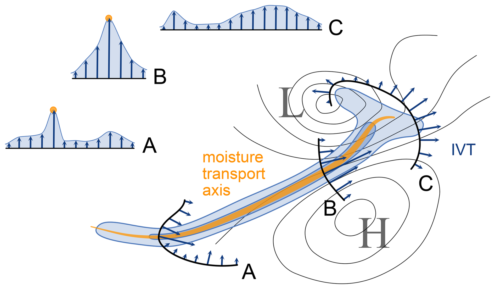
Figure 1 Illustration of the detection method. Blue shading and vectors show the magnitude and direction of the vertically integrated water vapour transport (IVT). The black lines marked A, B, and C are cross sections perpendicular to the local IVT direction. Well-defined maxima in the local IVT along the sections are marked by yellow circles in A and B; these well-defined maxima are then connected to form the yellow moisture transport axis line. Black contours indicate isobars, and the labels L and H mark a cyclone and an anticyclone, respectively.

In the second step, we filter out IVT minima and weak IVT maxima by requiring that

$$\begin{array}{}\text{(2)}& \left|\text{IVT}\right|\cdot {\displaystyle \frac{\partial {\mathit{\sigma }}_{\mathrm{IVT}}}{\partial n}}\le K_{\mathrm{IVT}},\end{array}$$

where K_IVT is a (negative) threshold that needs to be set. This criterion extracts well-defined maxima in the IVT using a combination of absolute magnitude ($\left|\text{IVT}\right|$) and sharpness of the IVT maximum ($\frac{\partial {\mathit{\sigma }}_{\mathrm{IVT}}}{\partial n}$). Small-amplitude maxima can thus become part of a moisture transport axis if the associated peak in IVT is sharp enough (yellow dots in the cross sections A and B in Fig. 1). Minima in IVT do not fulfil this criterion, because there $\frac{\partial {\mathit{\sigma }}_{\mathrm{IVT}}}{\partial n}$ > 0. For determining K_IVT, we follow the suggestion of Spensberger et al. (2017) and use the 12.5th percentile of year-round global $\left|\text{IVT}\right|\cdot \frac{\partial {\mathit{\sigma }}_{\mathrm{IVT}}}{\partial n}$. For ERA5, the resulting threshold is K_IVT = $-\mathrm{4.06}\times {\mathrm{10}}^{-\mathrm{7}}$ kg² s⁻² m⁻⁴. When applied to a climate model, the variation of this percentile across the climates to be studied will provide an indication of whether the threshold might need to be adapted. However, for simulations with the CESM2 model covering the period 1960 to 2100, Konstali et al. (2024a) found no need to adapt the threshold to account for the changing climate, underlining the advantage of defining moisture transport features based on their elongated structure.

In a third step, we connect all remaining points marking well-defined IVT maxima into lines using a maximum distance of 1.5 grid points between two successive points along a line (technical details on this step are in Spensberger et al., 2017). In the fourth and final step, we require a minimum length of 2000 km, measured following the line, for such a line to become a moisture transport axes (yellow line in Fig. 1). This minimum length is in line with typical geometrical constraints used for detecting atmospheric rivers (Rutz et al., 2019).

In all following snapshots, the resulting moisture transport axes are directly visualised as yellow and white lines. For visualising time-mean occurrence in climatologies and composites, we however find one additional step to be helpful. As lines do not have an areal extent, appropriate normalisation without further assumptions would result in the unit m⁻¹ for mean occurrence. This unit can be interpreted as an average line length per unit area (e.g. Spensberger and Spengler, 2020) but is still not intuitive. Thus, we use a 200 km radius to lend our lines an areal extent. Such a small radius hardly changes the geographical pattern, but the time-mean occurrence of this spatial feature becomes simply a dimensionless fraction of time steps in which a moisture transport axis is within 200 km of a given location.

2.3 Case studies from low, mid, and high latitudes

To illustrate the performance of the detection algorithm, we showcase selected occurrences of moisture transport axes (yellow lines in Fig. 2). Three of the four cases in Fig. 2 are based on previous studies of atmospheric rivers. The North Pacific and southern Indian Ocean cases are discussed in Lora et al. (2020) (our Fig. 2a–d). The North Atlantic case (Fig. 2e, f) is discussed in Azad and Sorteberg (2017) and yielded one of the highest daily precipitation totals on record in Bergen on the west coast of Norway. These cases also include examples of high-latitude moisture transport axes, such as the one touching the Antarctic coastline south of Africa (Fig. 2d) and the one close to Novaya Zemlya (Fig. 2f). The fourth case highlights a moisture transport axis from the Sahel region across the Sahara toward the Mediterranean (Fig. 2g, h). This moisture transport axis is associated with scattered patches of precipitation exceeding 1 mm h⁻¹ over the Sahara (pink contours in Fig. 2g).

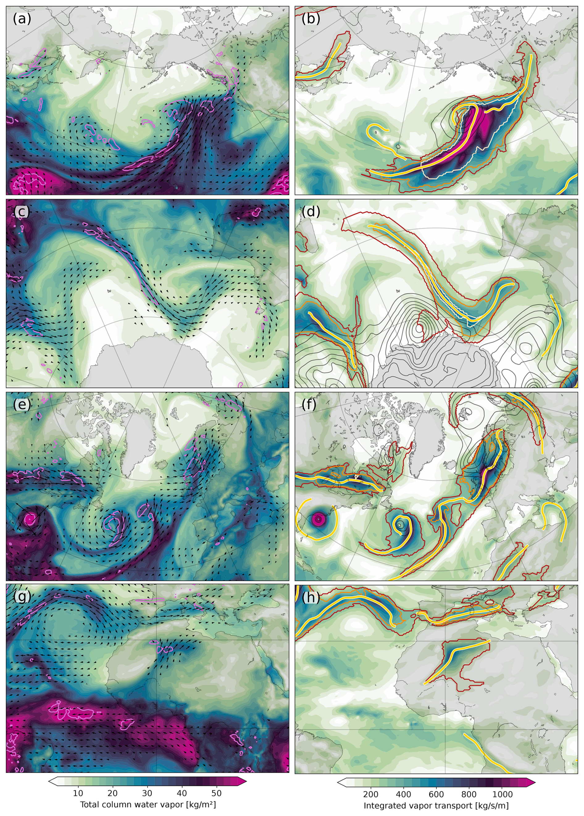
Figure 2 Snapshots of moisture transport axis occurrence. Panels (a)–(d) show atmospheric river cases discussed by Lora et al. (2020) on 5 November 2006, 09Z, and 14 November 2006, 09Z, respectively; (e, f) the strongest river case listed in Azad and Sorteberg (2017) on 14 September 2005, 00Z; and (g, h) a moisture transport axis over the Sahara on 15 December 2017, 06:00 UTC. The left column shows total column water vapour [kg m⁻²] (shading), IVT (arrows), and total precipitation (pink contour, 1 mm h⁻¹). The right column shows the magnitude of IVT [kg m s⁻¹]. Black contours show sea-level pressure below 1010 hPa in steps of 5 hPa. Red, orange, and pale red contours show the number of atmospheric river detections in the ARTMIP-ERA5 dataset with contours at 1, 3, and 6, respectively, of the six available global algorithms. Finally, the yellow lines show detected moisture transport axes.

At all latitudes, the showcased moisture transport axes clearly trace synoptic-scale maxima in the moisture transport (right column of Fig. 2), despite the large variation in the absolute magnitude of the IVT along the various axes and across the different climate zones. Many axes extend to IVT values below 250 kg s⁻¹ m⁻¹, and some trace IVT maxima beyond the saturation of the colour scale at 1150 kg s⁻¹ m⁻¹. For example, the moisture transport axes trace a moisture filament associated with only moderate IVT close to Novaya Zemlya in the Arctic, the cyclonic and nearly circular moisture transport around tropical cyclones (e.g. close to the North American east coast in Fig. 2f), moderate-intensity moisture transport filaments over northern Africa (Fig. 2f), and tropical moisture export into the much drier subtropics (Fig. 2h). Beyond synoptic-scale transports, moisture transport axes also highlight some mesoscale structures such as the diffluent moisture transport around the occlusion point of the cyclone in Fig. 2b.

3 Climatology of moisture transport axes

Climatologically, the occurrence of moisture transport axes in the mid-latitudes follows the storm tracks (Fig. 3; cf. Chang et al., 2002, and Wirth et al., 2018). This is particularly true for the winter hemisphere (Fig. 3a, c). During winter, the occurrence of moisture transport axes is closely related to the IVT climatology (grey contours in Fig. 3), whereas during summer and autumn moisture transport axes occur frequently over the continents downstream of a storm track despite comparatively small climatological IVT.

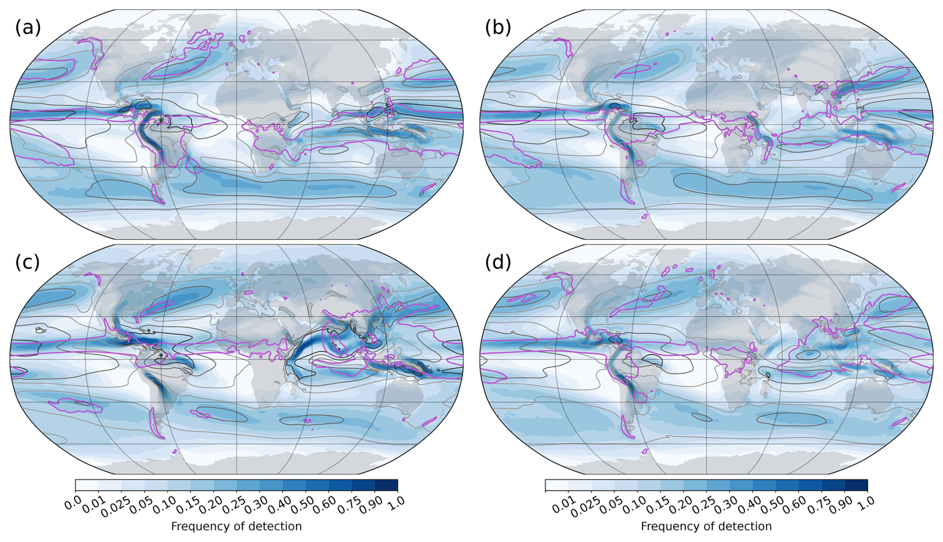
Figure 3 Climatological occurrence of moisture transport axes within 200 km of any given location for (a) DJF, (b) MAM, (c) JJA, and (d) SON. Grey contours show the climatological magnitude of the vertically integrated water vapour transport with contours at 100, 200, and 400 kg (m s)⁻¹, and the pink contour marks the region exceeding 5 mm d⁻¹ of total precipitation.

In the subtropics and tropics, the occurrence of moisture transport axes is confined to specific regions (Fig. 3). Moisture transport axes frequently occur along the Intertropical Convergence Zone (ITCZ) year-round. In addition, the monsoon circulation is frequently associated with moisture transport axes, e.g. the Indian monsoon (Fig. 3c) as well as the Somali Jet (moisture transport in the Somali Jet is discussed in detail in Viste and Sorteberg, 2013). The climatology of moisture transport axes also highlights the moisture transport along low-level jets steered by orography. This effect is apparent year-round along the South American low-level jet on the eastern side of the Andes (Montini et al., 2019) but also, with seasonal variation, along the straits through the Maritime Continent.

In comparison with the low and mid-latitudes, relatively few moisture transport axes occur in subpolar and polar regions (Fig. 3). Nevertheless, the 1 % frequency of occurrence isoline extends to around 80° N in the North Atlantic during winter (Fig. 3a), and the 5 % contour covers most of the ice-free Arctic Ocean during summer (Fig. 3c). Similarly, in the North Pacific, the Aleutian Islands have a moisture transport axis nearby for more than 5 % of the winter time steps. In the Southern Hemisphere, the 1 % isoline generally follows the Antarctic coastline during all seasons and extends furthest poleward upstream of the Antarctic Peninsula in the South Pacific sector. Over the ice sheets of Antarctica and Greenland, very few moisture transport axes are detected.

In synthesis, the case studies and climatologies give a strong indication that our definition of moisture transport axes is able to detect moisture filaments across all climate zones except the ice sheets. The detections appear to align well with the concept of atmospheric rivers in the mid-latitudes (a more stringent comparison follows in Sect. 4) but also capture synoptically meaningful events in the tropics, subtropics, and polar regions.

4 Mid-latitude moisture transport axes and their relation to atmospheric rivers

The climatologies of moisture transport axes resemble the consensus detection frequencies in the ARTMIP catalogue (compare our Fig. 3 with Fig. 5 of Collow et al., 2022). The most obvious difference between our results and the ARTMIP consensus is the frequency of detection in the subtropics and tropics. We observe a significant number of detections at low latitudes. These might not be desirable for all applications, and we thus explore the potential of reducing the number of tropical detections by normalising the IVT input fields in the Supplement. In the mid-latitudes, the results are, however, largely unaffected by normalisation (details in the Supplement).

The case studies in Fig. 2 also indicate a good correspondence between moisture transport axes and atmospheric rivers in the mid-latitudes. Specifically, our moisture transport axes correspond well to the six atmospheric river detection schemes available for ERA5 (red, orange, and pale contours in the right column of Fig. 2; cf. majority consensus detections for the cases in Fig. 4c and g of Lora et al., 2020).

In contrast to atmospheric rivers, however, moisture transport axes highlight the diffluent moisture transport close to the occlusion point of a cyclone (e.g. Fig. 2b). From the occlusion point, one branch of moisture transport typically spirals cyclonically toward the cyclone core, while another branch follows the warm front away from the cyclone core. These two branches likely correspond to the two types of warm conveyor belt outflow recently documented by Heitmann et al. (2024). In line with their findings, the dominant branch can vary from cyclone to cyclone (toward cyclone in Fig. 2b, away in Fig. 2d; both branches are evident in Fig. 2f). Not all fronts, however, are associated with a moisture transport axes (e.g. warm front south of South Africa in Fig. 2c, d). The co-occurrence of fronts and moisture transport axes may define frontal moist baroclinicity – a metric that combines relative humidity and the isentropic slope, describing one main dimension of variability between fronts (Spensberger and Sprenger, 2018).

To corroborate the qualitatively good correspondence between moisture transport axes and atmospheric rivers documented by the case studies and climatologies, we supplement these analyses first by a quantitative comparison of the properties of moisture transport axes with a selection of criteria that are sometimes used to identify atmospheric rivers (marginal histograms in Fig. 4) and second by a composite analysis of moisture transport axes making landfall in northern California.

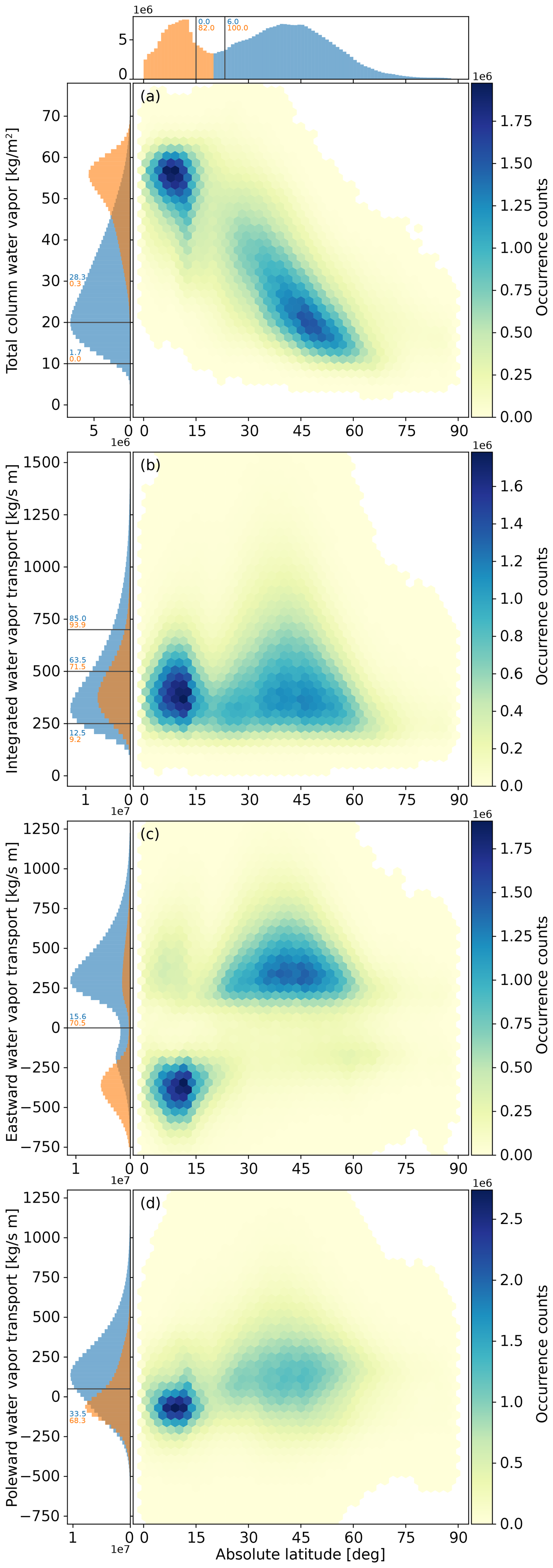
Figure 4 Two-dimensional histograms showing the occurrence counts of moisture transport axes in phase spaces defined by latitude and (a) total column water vapour and (b) magnitude of IVT, as well as (c) eastward and (d) poleward components of the IVT. One-dimensional histograms along the respective axes are displayed along the sides. We use a cutoff of 20° latitude to separate tropical (orange) from extratropical (blue) moisture transport axes in these histograms. Typical detection thresholds used for atmospheric river detections are indicated by lines across the one-dimensional histograms, with the adjacent numbers indicating the percentile at which these lines occur in the respective distributions.

The distribution of moisture transport axes across latitude is clearly bimodal with one narrow peak around 10° latitude as well as a wider peak centred around 45° latitude (Fig. 4a–d). The minimum in frequency of detections occurs around 20° latitude, close to the 15 and 23.25° cutoffs used in the atmospheric river detection schemes of Ullrich and Zarzycki (2017) and Shearer et al. (2020), respectively. We use a cutoff at 20° latitude to distinguish between tropical and extratropical moisture transport axes in the marginal histograms in Fig. 4.

The bimodality in latitude is reflected in a slight bimodality also in total column water vapour (TCWV; Fig. 4a). Tropical moisture transport axes are associated with distinctly more TCWV than extratropical moisture transport axes, with only a small overlap in the distributions around 45 kg m⁻². The most frequent TCWV in extratropical axes is approximately 20 kg m⁻², and 28 % of these axes are below this value. Note that the histogram is based on all points along all moisture transport axes rather than the axes' peak intensity. The statistic thus implies that 28 % of the combined length of all extratropical moisture transport axes is below the 20 kg m⁻² threshold.

Most detection algorithms for atmospheric rivers use IVT as one of their criteria to define the feature. Typical thresholds used are 250, 500, and 700 kg s⁻¹ m⁻¹ (e.g. CONNECT by Sellars et al., 2015; TempestExtremes by Ullrich and Zarzycki, 2017; and the Rutz et al., 2014, algorithm). In comparison, the most common IVT value along moisture transport axes is around 350 kg s⁻¹ m⁻¹ (Fig. 4b). Interestingly, the most common value is largely independent of latitude (Fig. 4b), such that tropical and extratropical transport axes are associated with similar IVT. The strongest IVT, beyond 700–800 kg s⁻¹ m⁻¹, does however mostly occur around 45° latitude. The vast majority (88 %) of the extratropical transport axes exceed the 250 kg s⁻¹ m⁻¹ threshold. At the same time, most of these axes are also located below the 500 and 700 kg s⁻¹ m⁻¹ thresholds (64 % and 85 %, respectively).

Instead of using a cutoff latitude, several definitions of atmospheric rivers rely on a threshold for the poleward and/or eastward component of the IVT (e.g. Guan and Waliser, 2015; Mattingly et al., 2018; Viale et al., 2018). The eastward component of the IVT also exhibits a bimodal distribution with a local minimum between the westerly and easterly modes at 0 kg s⁻¹ m⁻¹ (Fig. 4c). This bimodality maps reasonably well onto the bimodality in latitude, with tropical axes being mostly easterly and mid-latitude axes being mostly westerly. A separation using a threshold at zero nevertheless remains questionable, as there is still a substantial number of extratropical axes with easterly moisture transport (15 % of the total length) and vice versa (29 % of the tropical axes are associated with westward moisture transport).

Eastward transport in the extratropics happens most frequently around 60° latitude (Fig. 4c). From a synoptic perspective, this is most often associated with the easterlies on the poleward side of a cyclone (example in Fig. 2b) and along the Antarctic coastline. A further problem with a cutoff at 0 kg s⁻¹ m⁻¹ eastward IVT is the frequent occurrence of mainly meridional moisture transport in the Southern Hemisphere (e.g. Fig. 2d), where slight variations off the meridional direction then determine whether an atmospheric river is detected.

Similar arguments hold for the poleward IVT (Fig. 4d). Here, the distributions for both tropical and extratropical moisture transport overlap considerably with a zero poleward IVT threshold. Consequently, about a third of the extratropical axes exhibit equatorward moisture transport. Furthermore, the distributions of poleward IVT for tropical and extratropical transport axes show a large degree of overlap (histogram to the side of Fig. 4d), such that the poleward IVT component is not suitable to distinguish between tropical and extratropical moisture transport.

Despite the mentioned differences between moisture transport axes and typical definitions of atmospheric rivers, these two concepts generally capture the same phenomenon in the mid-latitudes. For example, the occurrence of moisture transport axes along the North American west coast is often associated with strong precipitation (snapshot and composite analysis in Fig. 5), and the characteristic synoptic structure associated with atmospheric rivers in this region (as documented in Fig. 9 of Rutz et al., 2019) is very similar to the mean synoptic situation conditioned on the presence of a moisture transport axes in the same location (Fig. 5c, d).

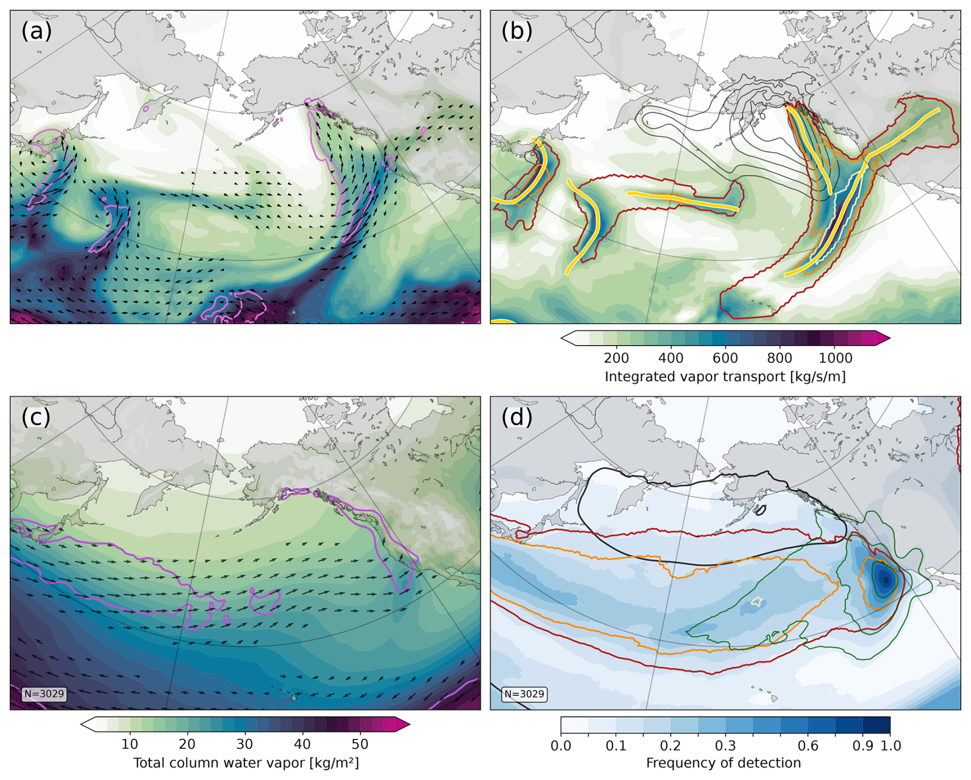
Figure 5 (a, b) Snapshot of an atmospheric river case from 15 February 2014, 09Z, discussed in Rutz et al. (2019) analogous to each row in Fig. 2. (c, d) Composites based on the occurrence of a moisture transport axis within 200 km of the position 34° N, 124° W. The target location is marked in panel (d) by a maximum in the detection frequency approaching 100 % and in panel (c) by a local maximum in TCWV. (c) Total column water vapour [kg m⁻²] (shading) with the grey contour highlighting the 20 kg m⁻² contour, IVT (arrows), and total precipitation (pink contour at 5 mm d⁻¹). (d) Frequency of occurrence of normalised moisture transport axes within 200 km. Dark green contours show the frequency of occurrence for only those moisture transport axes that intersect the target region (contours at 0.05, 0.1, 0.2, 0.4, 0.6, and 0.9). Black contours show sea-level pressure below 1010 hPa in steps of 5 hPa. Finally, red, orange, and pale red contours show the frequency at which more than half of the six available atmospheric river detections for ERA5 agree on the detection. Contours are at 5 %, 10 %, and 20 %, respectively. The composites are based on the period 2000–2019, as ARTMIP-ERA5 detections are generally only available for this period. For all other variables, composites for 1979–2020 would be nearly indistinguishable (not shown). The composites are not restricted to a particular season and thus follow the seasonality of the detected of moisture transport axes.

5 Polar moisture transport axes and their relation to warm moist intrusions

Moisture filaments and associated peaks in the moisture transport occur in a similar form also in polar regions (Woods et al., 2013). Gorodetskaya et al. (2014) and Wille et al. (2019) discuss cases where moisture filaments made landfall on the Antarctic coastline, referring to these features as atmospheric rivers to stress the similarities with their mid-latitude counterparts. Around Antarctica, atmospheric rivers are an important factor for both liquid and frozen precipitation (Gorodetskaya et al., 2014; Wille et al., 2019, 2021) and have also been linked to ice sheet calving events (Wille et al., 2022). When these moisture filaments occur in the Atlantic Arctic, they are typically called warm moist intrusions (e.g. Woods and Caballero, 2016; Papritz et al., 2022), although Mattingly et al. (2018) also use the label atmospheric river to conceptualise moisture transport onto the Greenland Ice Sheet. In the following, we relate detected moisture transport axes to both of these features, but we focus on maritime/coastal events, as we detect very few moisture transport axes over the ice sheets.

Returning first to the Southern Ocean and the May 2009 case of Gorodetskaya et al. (2014), a moisture transport axis traces the essentially meridional moisture transport across all of the mid-latitudes from close to Madagascar onto the Antarctic continent (Fig. 6a, b). Their February 2011 case is similar in that it also features a well-defined moisture transport axis across all of the mid-latitudes and is thus only shown in the Supplement (Fig. S1c, d). In both cases, the moisture transport is captured well by the detected axes but also largely by the ARTMIP schemes available for ERA5.

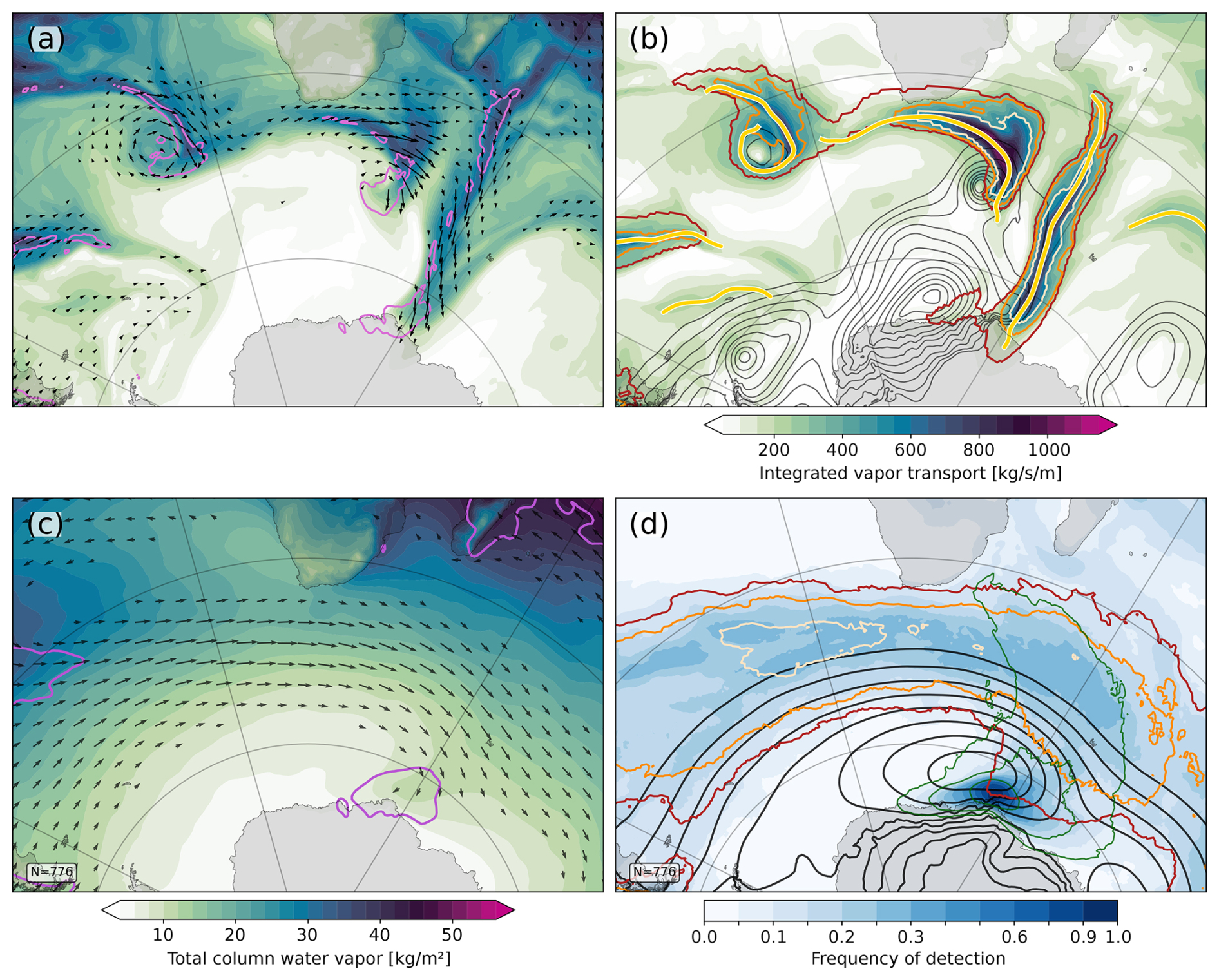
Figure 6 Same as Fig. 5 but for atmospheric rivers making landfall on Antarctica. The snapshot from 19 May 2009, 00Z (a, b), is one of the cases discussed in Gorodetskaya et al. (2014). The composite (c, d) is based on moisture transport axes occurring within 200 km of the landfall location.

The synoptic structure of the May 2009 case is typical for the region (Fig. 6c, d). A composite of all cases where moisture transport axes reach the Antarctic coastline within 200 km of the Gorodetskaya et al. (2014) case demonstrates a predominantly meridional orientation of the axes reaching the coastline (green contours in Fig. 6d). Few transport axes penetrate into the interior of the Antarctic continent; nearly all are diverted along the coastline (green contours and shading in Fig. 6d). In contrast, the composite moisture transport remains largely zonal throughout most of the mid-latitudes and only exhibits a cyclonic anomaly close to the Antarctic coast centred around 60° S (Fig. 6c). Many of these events are also captured by the ARTMIP-ERA5 schemes (orange and pale red contours in Fig. 6d), but ARTMIP detections are substantially less consistent for this location compared to northern California (Fig. 5d; peak detection rates of 20.4 % versus 28.8 %).

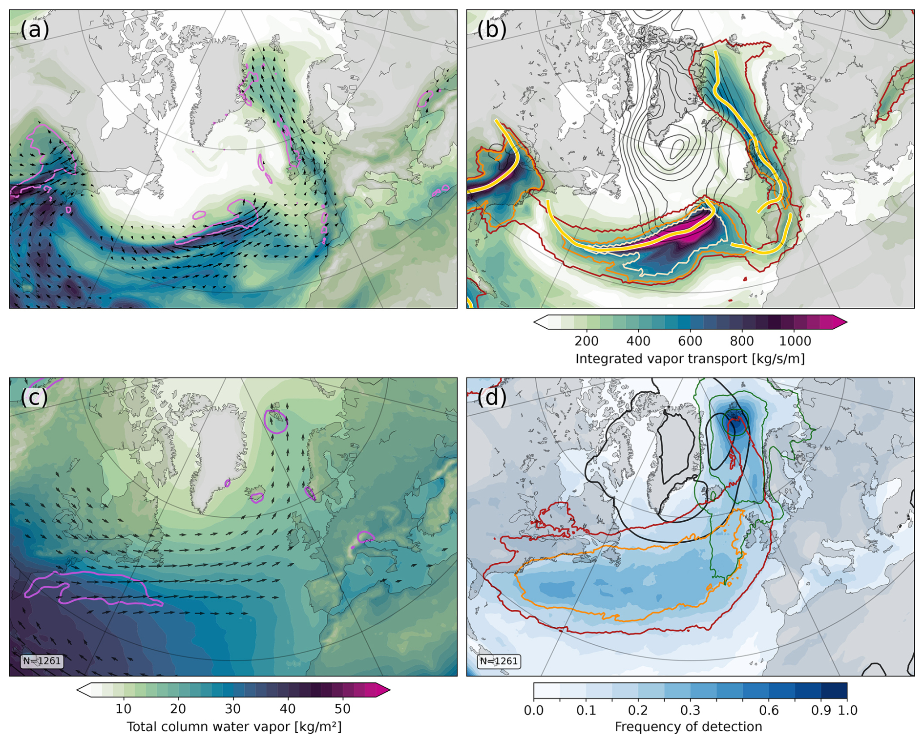
Figure 7 Same as Fig. 5 but for moisture transport axes around Svalbard. The snapshot from 29 December 2015, 00Z (a, b), is discussed in Binder et al. (2017). The composite (c, d) is based on moisture transport axes occurring within 200 km of Longyearbyen, Svalbard.

In the Atlantic Arctic, a moisture transport axis occurs in the vicinity of Longyearbyen between 1 % and 2.5 % of the winter time steps (Fig. 3a). In line with the findings of Serreze et al. (2015), a composite analysis of these events highlights pronounced northeastward moisture transport from the mid-latitude North Atlantic (Fig. 7). Moisture transport axes occur frequently across the entire subpolar North Atlantic, between Greenland and Norway, with only a slight skew toward the Norwegian coast. The composite is also fully consistent with the case study discussed in Binder et al. (2017), with pronounced meridional moisture transport between France and the Fram Strait (Fig. 7a, b).

These composites and synoptic examples suggest a good correspondence between our moisture transport axes and both polar atmospheric rivers and warm moist intrusions. To corroborate this finding, we systematically compare our transport axes with the occurrence of warm moist intrusions as defined by Woods et al. (2013). They define such intrusions by a transport threshold of 200 Tg d⁻¹ per degree longitude across 70° N, which corresponds to about 61 kg s⁻¹ m⁻¹. We relate this to the poleward IVT along all moisture transport axes detected between 68 and 72° latitude (Fig. 8c). We include detections within ±2° latitude to increase the sample size for this analysis.

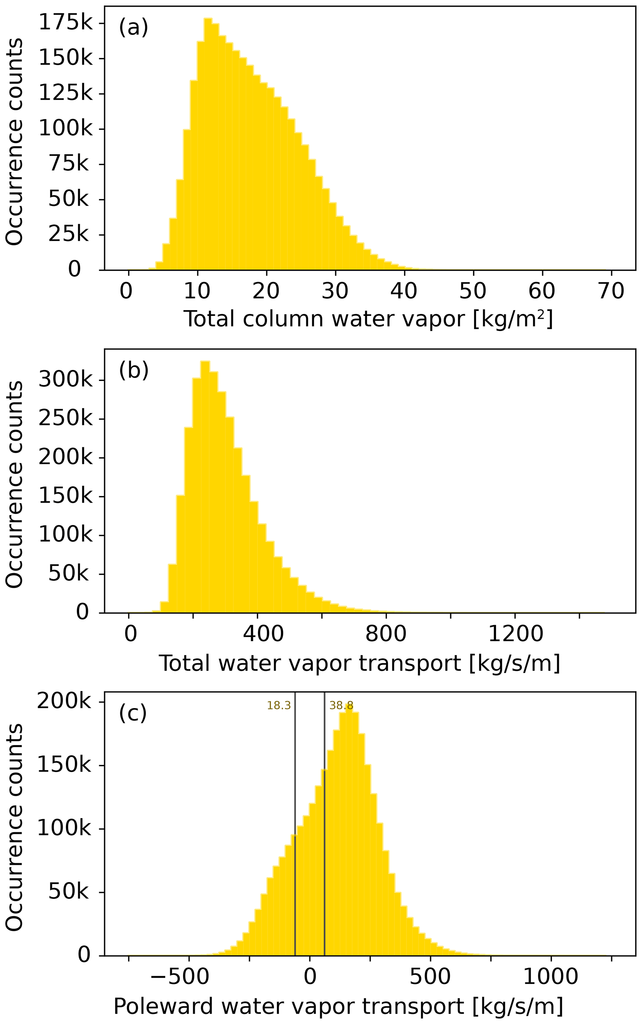
Figure 8 Same as the one-dimensional histograms on the left-hand side of Fig. 4a, b, and d but based on moisture transport axes detected within 68–72° N/S. For the relevance of the vertical lines and percentiles in panel (c), refer to the main text.

About 60 % of the transport axes exceed this threshold (Fig. 8c). Furthermore, a skew in the poleward IVT distribution toward positive values shows that moisture transport is predominantly poleward. Nevertheless, about 20 % of moisture transport axes around 70° latitude exceed a threshold of the opposite sign, signalling the regular occurrence of warm moist extrusions from the Arctic. This phenomenon has also been noticed by Papritz and Dunn-Sigouin (2020), who separated total and net moisture transport into the Arctic. Such emphasised moisture export from the Arctic is plausible from the synoptic example in Fig. 2f. In this snapshot, a moisture transport axis turns equatorward around 60° S, tracing the warm front of a mature cyclone. An analogous synoptic situation with a cyclone core located in the Barents Sea would simultaneously yield strong moisture import into and export from the Arctic.

Considering transport irrespective of direction, few transport axes feature less than 200 kg s⁻¹ m⁻¹ (Fig. 8b). Furthermore, while most polar transport axes feature TCWV below 20 kg m⁻², it is interesting to note the occasional occurrence of moisture transport axes with up to around 40 kg m⁻² even at around 70° latitude (Fig. 8a).

6 Tropical moisture transport axes and their relation to tropical moisture exports and monsoon air streams

The low-latitude case study and climatologies suggest varying dynamical reasons for the occurrence of moisture transport axes in the tropics and subtropics. Some seem to be steered by orography (e.g. across the Maritime Continent and along the Andes), some seem to capture intermittent moisture transport similar to that in the extratropics (e.g. Sahel region), and some seem to capture seasonal circulation anomalies like the Indian monsoon. The latter result is in line with Park et al. (2021) and Reid et al. (2022), who use atmospheric rivers to conceptualise variability in the East Asian and Australian monsoons, respectively. Interestingly, topographically steered moisture transport axes mostly vanish with normalisation (Fig. S2 in the Supplement), implying an almost continuous moisture transport in these regions. In contrast, the Indian, East Asian, and Australian monsoons remain visible with normalisation by the annual means (composite for the Indian monsoon in Fig. S2) but do largely vanish when normalising by the seasonal mean (not shown) due to the near-stationary flow during the monsoon season.

Using composite analyses, we contrast the moisture transport axes detected in the near-stationary Indian monsoon with the intermittent transport axes detected over the Sahel region (Fig. 9). The composite analysis for the Indian monsoon is based on the occurrence of transport axes in the vicinity of Kolkata, India. This composite comprises 8982 time steps, corresponding to about 56 d yr⁻¹, highlighting the semi-permanent nature of the feature during the monsoon season (Fig. 9b). The composite moisture transport axes are diverted by the Himalayas, with westward-pointing moisture transport axes along the mountain range to the west of the Bay of Bengal and eastward axes to the east (Fig. 9b). This diffluence is not visible in the direction of the mean transport (Fig. 9a), because the magnitude of the mean transport vector is relatively small along the Himalayas (grey contours in Fig. 9b). In combination with the high TCWV evident in Fig. 9a, this indicates a variable transport direction along the mountain range.

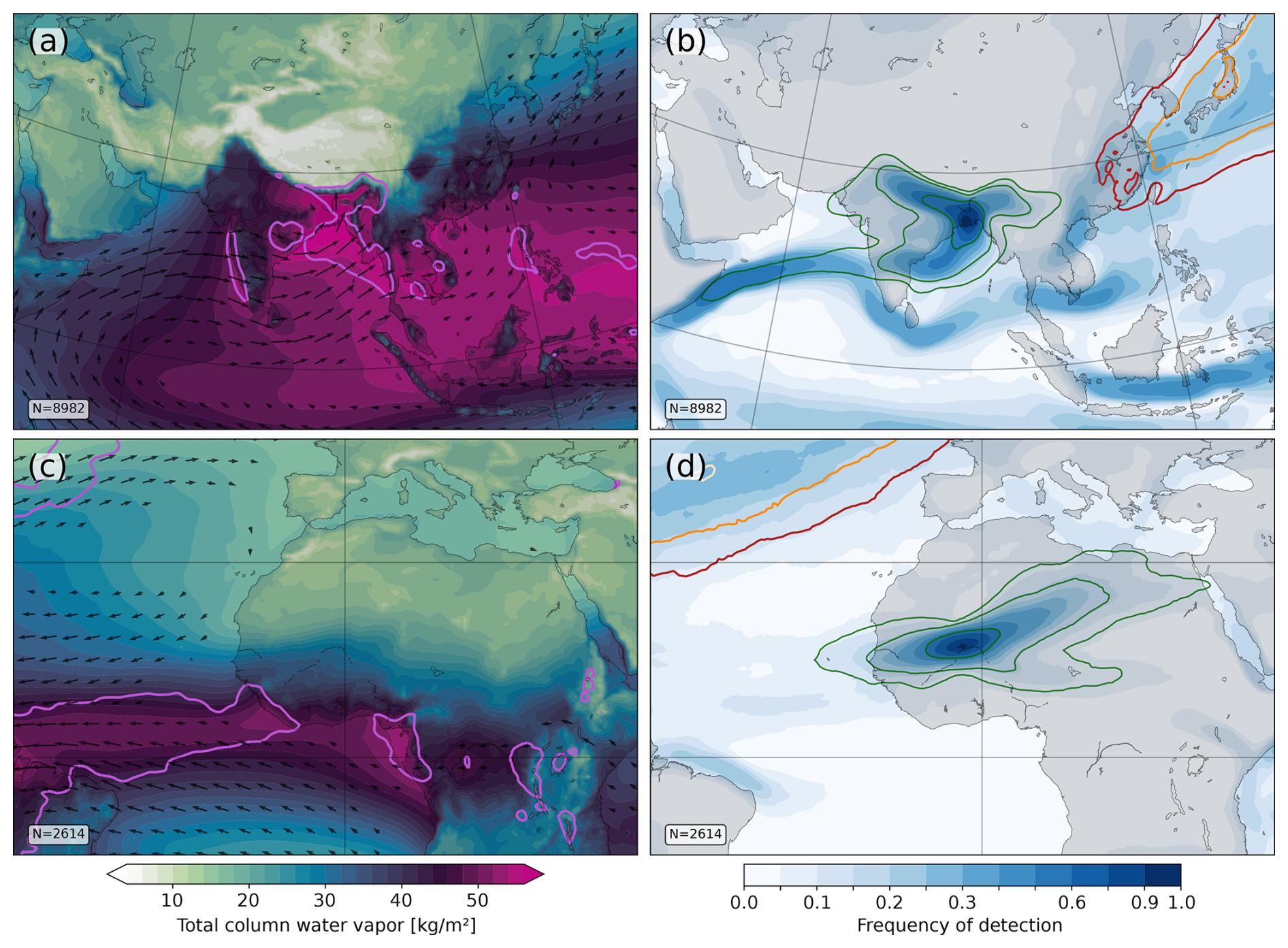
Figure 9 Same as the composites in Fig. 5c, d but (a, b) for moisture transport axes within 200 km of Kolkata, India, and (c, d) for moisture transport axes within 200 km of Timbuktu, Mali, in the Sahel region.

With our second composite analysis, we move from one of the (seasonally) most humid to one of the most arid places in the subtropics (Fig. 9c, d). Here, the composites are based on the occurrence of moisture transport axes close to Timbuktu, Mali, which is located in the Sahel belt to the south of the Sahara. The snapshot in Fig. 2g and h includes an example case included in this composite. In line with the snapshot, the composite structure shows a tilted export of moisture from the ITCZ into the Sahel region (Fig. 9c). Although the average precipitation along these transport axes is not strong enough to exceed the contour level, the snapshot in Fig. 2g and h illustrates that scattered precipitation can be associated with such transport events.

In the Sahel region, the occurrence of moisture transport axes is very intermittent, mainly occurring during late summer (JAS) and winter to early spring (DJFMA). The composite includes about 16 d yr⁻¹. Their occurrence during JAS coincides with the West African monsoon (e.g. Sultan and Janicot, 2003; Maranan et al., 2018) and the occurrence of African easterly waves (e.g. Berry et al., 2007). In contrast, the occurrence during winter and spring might be related to an influence from the mid-latitudes due to the southward displacement of the storm track (e.g. Knippertz, 2007; Spensberger and Spengler, 2020; Armon et al., 2024).

7 Summary and concluding remarks

We introduced a novel and generic feature detection algorithm for moisture filaments using an algorithm developed to detect upper-tropospheric jets (Spensberger et al., 2017). We call the detected features moisture transport axes, as these trace lines of maximum vertically integrated moisture transport (IVT). The name moisture transport axes and the visualisation as lines are not meant to imply a continuous transport along the line. As Läderach and Sodemann (2016) and Dacre et al. (2019) pointed out, there is a continuous recycling of water along atmospheric rivers, even though some long-range transport of moisture does occur (Stohl et al., 2008; Sodemann and Stohl, 2013). Analogously, we expect the same to be true for moisture transport along our detected moisture transport axes.

Conceptually, moisture transport axes strike a balance between Eulerian two-dimensional atmospheric river detections and the Lagrangian definitions of moist air streams that exist for tropical moisture exports (Knippertz and Wernli, 2010) and warm conveyor belts (Madonna et al., 2014), respectively. Compared to atmospheric rivers, moisture transport axes offer a more structure-based definition at the cost of making it less straightforward to relate moisture transport axes to, for example, poleward vapour transport or precipitation. Within an atmospheric river body, these variables can simply be summed up to estimate the contribution of atmospheric rivers to the respective climatology, whereas a more sophisticated approach to attribution (e.g. Konstali et al., 2024a, b) is required for the moisture transport axis lines. Compared to Lagrangian air stream definitions, our Eulerian approach is both more generic and (much) less computationally expensive, while still highlighting similar features in a similar manner. However, moisture transport is not necessarily parallel to the line of IVT maxima. Neither is it necessarily aligned with the direction in which the atmospheric river or moisture transport axis is propagating. Furthermore, moisture transport axes are not parcel trajectories and thus do not share their conservational properties.

In the mid-latitudes, moisture transport axes generally capture the same synoptic phenomenon as commonly used definitions of atmospheric rivers. Due to the structure-based definition of the feature, moisture transport axes often trace the moisture filament further into the subtropics, continents, or polar regions than the ARTMIP detections available for ERA5. Consequently, moisture transport axes often also detect warm conveyor belts (Madonna et al., 2014) and highlight which of the Heitmann et al. (2024) outflow branches is dominant. Furthermore, moisture transport axes reveal the substructure of atmospheric rivers, with several distinct maxima in the IVT, and they are not subject to any limitations in the orientation of the moisture transport.

For polar regions (except the ice sheets), we document a relation to warm moist intrusions and to existing polar adaptations of atmospheric rivers. Moisture transport axes thus highlight events with pronounced moisture import into polar regions. They, however, also reveal synoptic structures where much of the imported moisture is directly exported again. While such events are implicitly accounted for in the analysis of Papritz and Dunn-Sigouin (2020), the existence of such moisture export events is not obvious from previous studies on warm moist intrusions.

In the tropics and subtropics, moisture transport axes highlight both intermittent, seasonal, and near-stationary features of the circulation. For example, moisture transport axes both highlight the continuously strong moisture transport in the Indian monsoon circulation and its transient peaks. In the climatologically arid Sahel region, moisture transport axes reflect intermittent tropical moisture exports as discussed in Knippertz and Wernli (2010). Finally, moisture transport axes trace the orographically steered South American low-level jet as well as moisture transport along the straits of the Maritime Continent. While these highlights are far from providing a comprehensive view of tropical moisture transports, they clearly suggest that the concept of moisture transport axes remains meteorologically meaningful also in these regions.

In conclusion, our approach allows us to unify atmospheric rivers, warm moist intrusions, tropical moisture exports, and monsoon air streams into one common concept: moisture transport axes. As our definition is based on the typically elongated structure of moisture transport, our detection algorithm performs seamlessly from the tropics across the mid-latitudes into the polar regions. The concept of transport axes might thus turn out to be particularly useful to study moist interactions between the tropics, subtropics, mid-latitudes, and polar regions. Furthermore, as our definition does not require changes to thresholds or a time-dependent normalisation, our definition of moisture transport axes has turned out to be more robust across varying climates than commonly used definitions of atmospheric rivers (Konstali et al., 2024a). Finally, following the approach of Spensberger and Spengler (2020), moisture transport axes enable the investigation of variability in the occurrence of atmospheric rivers largely independent from their varying intensity.