Seasonal to decadal variability and persistence properties of the Euro-Atlantic jet streams characterized by complementary approaches

Recent studies have highlighted the link between upper-level jet stream dynamics, especially the persistence of certain jet configurations, and extreme summer weather in Europe. The weaker and more variable nature of the jets in summer makes it difficult to apply the tools developed to study them in winter, at least not without modifications. Here, to further investigate the link between jets and persistent summer weather, we present two complementary approaches to characterize the jet dynamics in the North Atlantic sector and use them primarily on the Northern Hemisphere summer circulation.

First, we apply the self-organizing map (SOM) clustering algorithm to create a 2D distance-preserving discrete feature space for the tropopause-level summer wind field over the North Atlantic. The dynamics of the tropopause-level summer wind can then be described by the time series of visited SOM clusters, in which a long stay in a given cluster relates to a persistent state and a transition between clusters that are far apart relates to a sudden considerable shift in the configuration of upper-level flow.

Second, we adapt and apply a jet core detection and tracking algorithm to extract individual jets and classify them into the canonical categories of eddy-driven and subtropical jets (EDJs and STJs, respectively). Then, we compute a wide range of jet indices for each jet category for the entire year to provide easily interpretable scalar time series representing upper-tropospheric dynamics.

This work will focus on the characterization of historical trends, seasonal cycles, and persistence properties of the jet stream dynamics, while ongoing and future work will use the tools presented here and apply them to the study of connections between jet dynamics and extreme weather.

The SOM allows the identification of specific summer jet configurations, each one representative of a large number of days in historical time series, whose frequency or persistence had increased or decreased in the last few decades. Detecting and categorizing jets adds a layer of interpretability and precision to previously and newly defined jet properties, allowing for a finer characterization of their trends and seasonal signals.

Detecting jets at pressure levels of maximum wind speed at each grid point instead of in the dynamical tropopause is more reliable in summer, and finding wind-direction-aligned subsets of 0 contours in a normal wind shear field is a fast and robust way to extract jet cores. Using the SOM, we isolate persistent circulation patterns and assess if they occur more or less frequently over time. Using properties of the jets, we confirm that the Northern Hemisphere summer subtropical jet is weakening, that both jets get wavier, and that these jets overlap less frequently over time. We find no significant trend in jet latitude or in jet persistence. Finally, both approaches agree on a rapid shift in the subtropical jet position between early and late June.

1 Introduction

Extratropical tropopause-level jet streams are narrow bands of westerly winds and are one of the most prominent features of the upper-tropospheric circulation. Their large variability at a daily timescale (Woollings et al., 2014) along with their link to extreme weather (e.g., Martius et al., 2006; Mahlstein et al., 2012; Harnik et al., 2014) makes them an important object of research in meteorology and atmospheric dynamics.

From a climatological perspective, jet streams are often separated into two categories based on their location and momentum source (Kållberg et al., 2005; Koch et al., 2006; Harnik et al., 2014; Winters et al., 2020; Spensberger et al., 2023). The subtropical jet (STJ) is located at the poleward edge of the Hadley cell. It draws its momentum from the thermally driven Hadley cell circulation and is mainly confined to high levels, typically between 400 and 150 hPa (Krishnamurti, 1961; Held and Hou, 1980). The eddy-driven jet (EDJ) can be found further poleward, inside the Ferrel cell. It is also referred to as the subpolar or extratropical jet. It is driven by momentum flux convergence associated with midlatitude synoptic eddies (Palmen and Newton, 1948; Held, 1975; Schneider, 1977; Woollings et al., 2010). It has a much deeper vertical extent, typically extending below 700 hPa. The separation into STJ and EDJ is not always clear, as both sources of momentum are often present to varying degrees to drive either jet and depend on each other (Lee and Kim, 2003; Martius, 2014).

Certain features and configurations of the jet have received particular attention over the last few years due to their links to other aspects of the circulation, surface weather, or both. The latitude of the low-level EDJ has been identified as a major mode of variability of the wintertime Atlantic circulation (Athanasiadis et al., 2010; Woollings et al., 2010; Hannachi et al., 2012). A very zonal EDJ (low tilt) paired with a north-shifted STJ can create a rare but very persistent circulation pattern with a merged jet (Harnik et al., 2014). An instantaneously meandering jet is the marker of Rossby waves (e.g., Vallis, 2017), but strong narrow jets can act as waveguides for them too (Hoskins and Ambrizzi, 1993; Martius et al., 2010; Wirth, 2020; White and Mareshet Admasu, 2025). A locally sinuous jet may also mark the presence of a block (e.g., Nakamura and Huang, 2018; Woollings et al., 2018b). Jet properties also interact with each other. For instance, in winter, the EDJ's latitude influences its persistence and predictability (Franzke and Woollings, 2011; Barnes and Hartmann, 2011), and a jet with low speed has a higher daily variability in its waviness and latitude (Woollings et al., 2018a), which is hypothesized to favor blocks. Jet properties have also been linked to extreme events. The position of the EDJ modulates the odds of extreme events in the midlatitudes (Mahlstein et al., 2012), and so does its waviness (Röthlisberger et al., 2016b; Jain and Flannigan, 2021). Over Eurasia, the persistent simultaneous presence of the EDJ and STJ is associated with increased odds of extreme heat in summer in certain regions of western Europe (Rousi et al., 2022). Recently, statistical models trained on time series of a few (5–10) wintertime EDJ properties (introduced by Barriopedro et al., 2023) were used to skillfully predict air stagnation (Maddison et al., 2023) and temperature extremes (García-Burgos et al., 2023).

Climate change is expected to affect the jet streams in several ways. Through connections highlighted in the previous paragraph, themselves potentially affected by climate change, trends in jet stream properties may translate into trends in various aspects of atmospheric circulation and surface weather (e.g., Held, 1993; Stendel et al., 2021). The poleward shift of the jet streams under climate change was hypothesized very early on (e.g., Held, 1993). It is now observed in historical data in the global mean, albeit more clearly in winter than in summer and mostly for the EDJ. However, the signal is weak in the North Atlantic sector (Woollings et al., 2023). This poleward shift is projected to continue in future simulations (Barnes and Polvani, 2013; Lachmy, 2022; Woollings et al., 2023). For the STJ, the historical trend is season- and region-dependent. For the North Atlantic sector, Totz et al. (2018) report a poleward trend in the transition seasons and an equatorward trend in summer. The North Atlantic STJ is also weakening with time, especially in summer (Woollings et al., 2023; D'Andrea et al., 2024), and the North Atlantic EDJ has also been weakening in the last 2 decades (Francis and Vavrus, 2012; Woollings et al., 2018a), although an opposite trend has been observed for longer time periods (Blackport and Fyfe, 2022). In future simulations, a positive trend is projected for the maximum speed of the EDJ core, although this signal is not yet apparent in historical data (Shaw and Miyawaki, 2024). In past data and using three different metrics, Francis and Vavrus (2015), Di Capua and Coumou (2016), and Martin (2021) all find slight increases in EDJ waviness, but a stable STJ waviness was found in the last cited paper. Further downstream, however, Lin et al. (2024) find an increase in waviness for the Asian jet that has an Atlantic origin. By contrast to past trends, for future winters, Peings et al. (2018) find a decrease in waviness accompanied by a strengthening and squeezing of the EDJ. This opposite trend in EDJ waviness for past and future data is consistent with the findings of Cattiaux et al. (2016), who find a slight increase in waviness in the past only for certain basins (including the North Atlantic) and seasons but an overall decrease in waviness in future simulations. The conflicting results in jet meandering depending on the period and metric chosen were highlighted by Blackport and Screen (2020) and overall remain a subject of discussion in the community (Geen et al., 2023).

Most of the current research in atmospheric science requires reducing the complexity of the circulation from time-varying 2D or 3D fields to a smaller feature space. These simplified feature spaces are either continuous, like jet indices (Woollings et al., 2010; Di Capua and Coumou, 2016; Barriopedro et al., 2023) or the projection of instantaneous fields on principal components, or discrete, like weather regimes (e.g., Michelangeli et al., 1995) or other types of clustering methods like the self-organizing map (SOM; Gibson et al., 2017; Weiland et al., 2021; Rousi et al., 2022; Stryhal and Plavcová, 2023). These methods can also be categorized based on the number of choices the user needs to make, from statistical, e.g., dimensionality reduction or clustering, to expert-defined, e.g., jet indices, blocking indices, or wave-breaking indices. Statistical approaches are typically less fallible since they require fewer choices, but they tend to be harder to interpret than expert-defined features. Certain statistical methods are also known to produce physically unrealistic patterns that can lead to wrong interpretations (Monahan and Fyfe, 2006).

Here, to lay the groundwork for further research on all the interactions between jet streams and other large-scale circulation features or surface weather events, we develop two complementary diagnostic tools for the jet streams. Using two methods allows us to view the circulation from different angles and to combine the strengths of statistical and expert-defined approaches. Recently, Madonna et al. (2017) recommended the use of different, complementary, and problem-dependent approaches to describe the jet streams. Both of the diagnostic tools presented in this work are adaptations of existing techniques widely used in the field of atmospheric sciences, with implementation details changed and tailored for the specific needs of summertime, upper-level circulation.

The first one is the self-organizing map, a clustering algorithm. The SOM creates a distance-preserving discrete feature space that makes it a valuable tool to study stationarity and recurrence (Tuel and Martius, 2023), a major factor in extreme events. The second one is a set of jet characteristics computed on individual jet cores that are extracted, tracked, and categorized from wind fields. This provides a collection of continuous interpretable time series representing the jets over time.

After presenting both techniques in detail, we demonstrate their capabilities on reanalysis data. This work focuses more on summer than on the rest of the year. This season receives less attention when designing methods to characterize the circulation but is very important for extreme events and presents interesting, different trends compared to the rest of the year (Harvey et al., 2023). The SOM will only be trained on June, July, and August (JJA) days, but the jets are detected using year-round data to provide more context for the JJA results.

The seasonal variability of the upper-level circulation is characterized using both the week-by-week mean pathway through the SOM and the seasonal cycle of the jet properties, and interannual trends are assessed for state occurrence frequencies as well as for individual jet properties such as jet waviness. The SOM approach is related to the more established weather regimes, as their connections to weather impacts have been thoroughly studied. Finally, the persistence of the upper-level flow, characterized by both state persistence using the SOM and feature lifetime using jet tracking, is quantified. These preliminary results are in preparation for future work delving deeper into the comparison between these two, sometimes diverging, notions of persistence.

2 Data and methods

2.1 Data

We use 6-hourly gridded fields for the 1959–2022 period, over the 80° W–40° E and 15–80° N domain, extracted from the European Centre for Medium-Range Weather Forecasts reanalysis version 5 (hereafter, ERA5 reanalysis; Hersbach et al., 2020). The main variables we use are the horizontal wind components u and v and the wind speed U = $\sqrt{u^{\mathrm{2}}+v^{\mathrm{2}}}$, on the six following pressure levels: 175, 200, 225, 250, 300, and 350 hPa.

Both algorithms take as input, at each time step, 2D (longitude–latitude) fields of upper-tropospheric wind. We flatten the three wind fields (u, v, and U) in the vertical by retaining, at every grid point, their value at the pressure level where U is maximal since our goal is to detect jet cores, and they are defined as local wind speed maxima. We keep track, in a separate 2D field, of that pressure level to use later in the jet categorization. Both methods then add different preprocessing steps to this vertical maxima data, which will be discussed in the relevant sections.

We additionally use the potential temperature on the surface of maximum wind speed and the horizontal wind speed magnitude at the 500 hPa pressure level. Finally, summer Euro-Atlantic weather regimes (Cassou et al., 2005; Grams et al., 2017) are computed from 500 hPa geopotential height anomalies from ERA5, computed relative to a daily climatology including all years from 1959 to 2022 and smoothed with a 15 d centered rolling window.

2.2 SOM clustering

2.2.1 Definition

The self-organizing map (SOM) is a clustering method first introduced by Kohonen (1982) (see also Kohonen, 2013, for an in-depth review), whose main appeal over simpler predecessors like k means is the creation of a 2D distance-preserving discrete feature space. The SOM may be presented as a modification of k means. In k means, data points are split into k groups called clusters such that the variance within the clusters is minimal and the variance between clusters is maximal. Each cluster is then represented by the mean of all its members, called the cluster center or sometimes weight matrix. The SOM adds another layer to this algorithm, by placing the clusters on the nodes of a regular 2D grid of size k = n×m, typically rectangular or hexagonal, and has a distance metric on this discrete space, for example the Euclidean distance between nodes. There, a cluster i is defined by its weight matrix w_i, which is not equal in general to its center but is rather the result of a training process during which clusters on neighboring nodes have an influence modulated by the distance between nodes. Hereafter, we conflate the clusters and the nodes they sit on, and the phrases “distance between clusters” and “neighboring clusters” are to be understood as “distance between the nodes on which the clusters sit” and “clusters on neighboring nodes”, respectively.

The training then has a similar objective to k means, with the additional constraint that a pair of neighboring clusters should be more similar to each other than a pair of distant clusters. This constraint ensures the distance-preserving property of the created phase space. The desired similarity of neighboring clusters may be enforced by the choice of an appropriate neighborhood function. The neighborhood function, typically a Gaussian, is a parametric function with parameter σ, the neighborhood radius, and is applied to the distance between clusters in the training process. The convergence of the algorithm relies on decreasing σ, equivalent in our case to the Gaussian's scale parameter, over time during the training. However, the initial and final σ values as well as the decay function are additional choices that need to be made. In general, a larger σ allows for more similar neighbors, and the limiting case σ → 0 is equivalent to k means.

Both the SOM and k means share the same challenge, that is the choice of the number of clusters k. The SOM further adds the choice of the shape of the grid, k = n×m.

Allowing neighboring clusters to be similar can lead the SOM to be a worse clustering algorithm, in the usual sense of cluster separation, than k means if the neighborhood radius is different from zero at the end of training (Gibson et al., 2017). Its strength resides in the creation of a distance-preserving feature space. One of the reasons we use SOM is the interpretability of the trajectory when expressed as a succession of cluster visits. Once the SOM is trained, each time step is assigned to a cluster, its “best matching unit” or BMU, defined as BMU(t) = argmin${}_i\Vert {\mathbf{x}}_t-{\mathbf{w}}_i\Vert$, with x_t being the wind field at time step t. Thus, the input time series is represented as a succession of stays in clusters and jumps between clusters, where long stays or short jumps point to persistence, and long jumps indicate abrupt changes in the configuration of the upper-level flow.

2.2.2 Specific implementation

For the SOM algorithm, the June–July–August (JJA) vertically maximum wind speed field (see Sect. 2.1) is coarsened to a 1.5° resolution grid to reduce the computational complexity and to focus on the larger-scale features. However, the final results are shown at the initial 0.5° resolution. This is done by representing clusters with their centers, computed with the original higher-resolution data, rather than their weights.

The grid (of size n × m) is hexagonal with periodic boundary conditions and is associated with a discrete distance metric. As a consequence, clusters are at a unit distance away from their nearest neighbors, and the bottom row and left column are at a unit distance away from the top row and right column, respectively (see Fig. 1), such that each and every cluster has six neighbors, all at a unit distance. Periodic boundary conditions were chosen to avoid creating artificial over-representation of the central clusters, which would have diminished the relevance of our persistence measures later on. The SOM is initialized using the first two principal components of the input data to ensure reproducibility, as recommended in Kohonen (2013). Before training, the data are standardized and weighted by the cosine of latitude. We use the single-batch training algorithm (Kohonen, 2013), repeated 50 times with the neighborhood radius σ exponentially decaying from 2 to 0.2. This training algorithm does not involve a learning rate.

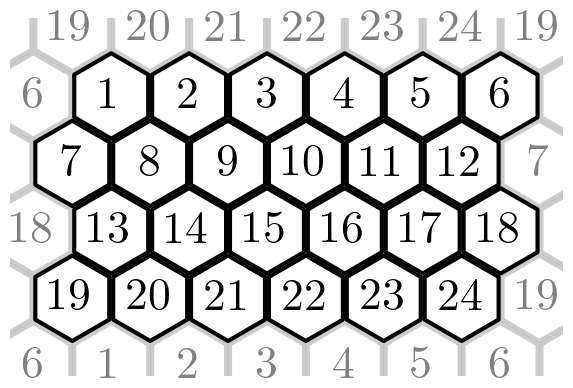
Figure 1 Hexagonal topology SOM with ideal grid size. The SOM clusters are in black, and the gray clusters illustrate the periodic boundaries.

To inform our decision regarding the SOM grid size, we use two performance metrics of the SOM. The first one is the energy function E of the SOM based on Heskes (1999) (see Eq. 1), and the second one is the 5th percentile of the projection of data points on their BMUs, defined as P in Eq. (2). These metrics are a function of the ensemble of SOM weights W = $\mathit{\{}{\mathbf{w}}_i,\mathrm{1}\le i\le n\times m\mathit{\}}$, and the ensemble of input data vectors x∈X, of size N, as well as the topological properties of the SOM. The grid distance between two SOM clusters i and j is precomputed and stored in a matrix of elements d_ij. These distances are then transformed by the neighborhood function to obtain the pairwise neighborhood parameters h_ij = f(d_ij;σ) based on the SOM's neighborhood radius σ. In this work, f is a zero-mean Gaussian with scale parameter σ.

$$\begin{array}{}\text{(1)}& {\displaystyle }E\left(W\right)={\displaystyle \frac{\mathrm{1}}{N}}\sum _{\mathbf{x}\in X}\underset{\mathrm{1}\le i\le n\times m}{min}\sum _{j=\mathrm{1}}^{n\times m}{h}_{ij}\Vert \mathbf{x}-{\mathbf{w}}_j{\Vert }^{\mathrm{2}}\text{(2)}& {\displaystyle }P\left(W\right)=\underset{\mathbf{x}\in X}{Q_{\mathrm{5}}}\left(\underset{\mathrm{1}\le i\le n\times m}{max}{\displaystyle \frac{\mathbf{x}\cdot {\mathbf{w}}_i}{\Vert \mathbf{x}\Vert \Vert {\mathbf{w}}_i\Vert }}\right)\end{array}$$

The goal is to minimize E and maximize P while maintaining a reasonably low number of clusters. The E and P objectives are similar, but the latter allows one to explicitly limit how poor the poorest projections on the SOM clusters are, making sure that most days are well-described in the 2D feature space described by the SOM since current and future work includes working on extreme configurations of the upper-level circulation. Testing for many sizes ranging from 4 × 4 to 9 × 9 was performed, and the chosen size is 6 × 4.

2.2.3 SOM metrics

We compute statistical properties from the trained SOM, including the populations of each cluster and their annual trends, two quality metrics, and the average and maximum residence time in a given cluster.

The first SOM metric of note is an analogue to the persistence index in dynamical systems theory. The average residence time at a given cluster i is simply given by the average length of time during which BMU(t) = i, starting at the transition from another cluster to i. The definition can be loosened to the length of time during which BMU(t) remains within a given distance of i. With a large SOM, which sometimes features minute differences between neighboring clusters, this second definition with a small distance can be a more realistic measure of persistence. To account for varying degrees of similarity between neighboring clusters, we do not use the discrete grid distance between clusters but instead use the Euclidean distance between SOM cluster weight matrices. At the start of JJA, the first stay starts on the first populated cluster, i₀. The stay continues if BMU(t) is on i₀ or any other cluster whose weight matrix has a distance from i₀ that is within the 10th percentile of inter-cluster-weight distances. When BMU(t) no longer respects this condition, a new stay begins at a new cluster i₁. The stay is associated with the most visited cluster during the stay, which is not necessarily the starting one.

We provide two cluster-wise quality metrics. The first one is the root mean square error (RMSE), defined for each cluster as the mean Euclidean distance between its weight matrix and its members. A low RMSE is preferred. The second quality metric is the cluster separateness. We compute, for each pair of clusters, the ratio of the Euclidean distances between their weight matrix to the grid distance that separates them. We then average all the ratios for all the pairs containing cluster i to obtain cluster i's separateness. High separateness is preferred.

Finally, we will relate our SOM clustering to the summer Euro-Atlantic weather regimes. Following Grams et al. (2017) but using only four weather regimes, we assign one of four weather regimes to each day of summer if the associated weather regime index is bigger than that of the three other regimes for at least 5 consecutive days and is above its temporal standard deviation within this time span. With this definition, 40 % of the time steps are not assigned to any weather regime. We then count the number of time steps previously assigned to a SOM cluster that are now also assigned to a weather regime.

2.3 Feature detection and tracking

The SOM is a powerful clustering tool to characterize the circulation as a whole in a given region. However, one might want to know more specific information about some of the components of the circulation, expressed as numbers rather than features on a composite map. We now turn to the methods we use to detect jets in vertical maximum 2D wind fields, to separate them into broad categories, to track them over time to assess their lifetime and evolution, and finally to extract a wide range of properties out of them. Thanks to seasonally varying thresholds (see Sect. 2.3.1), our method works equally well across the year. Therefore, we apply it to the full dataset rather than only to JJA, which will allow us to broaden the discussion of interannual trends to other seasons and paint a full picture of the jets' annual cycles.

2.3.1 Jet detection

Our jet detection algorithm is an adapted version of the method by Spensberger et al. (2017, hereafter S17). It can be applied to each time step independently, allowing for parallelization.

The vertical maximum wind speed fields (u, v, and U; see Sect. 2.1) are coarsened to a grid of 1.5°. Our choice of 2D fields, the level of maximum wind speed over several pressure levels, as described in Sect. 2.1, is the first difference from S17, who used wind fields interpolated onto the 2 PVU surface, where 1 PVU = 10⁻⁶ K kg⁻¹ m² s⁻¹. Internal testing has shown that the STJ is often undetectable on the 2 PVU surface in JJA, while it clearly appears on our 2D fields. The main criterion used to find jets is the horizontal normal wind shear $\mathit{\tau }:=\frac{\partial U}{\partial n}$ = $\frac{v}{U}\frac{\partial U}{\partial x}-\frac{u}{U}\frac{\partial U}{\partial y}$. Following Berry et al. (2007), τ = 0 is a necessary condition for a jet. The first step of this algorithm is thus to find contours of τ = 0, using a contour detection routine.

The points along the contours are filtered using a wind speed and an alignment threshold. We use the day-of-year climatological 75th percentile of 6-hourly wind speed as the wind speed threshold, so the algorithm works equally well in all seasons. The contour must also be aligned with the wind speed. This is done by computing the local tangent vector t = $\frac{\mathrm{d}\mathbf{x}}{\mathrm{d}s}$ with the linear path coordinate s and computing the alignment dot product a = $\frac{\mathit{t}}{\Vert \mathit{t}\Vert }\cdot \frac{\mathbf{u}}{U}$, as done in Molnos et al. (2017). We require a > 0.3 for a jet. With very few values of a different from either −1 or +1, the performance of the algorithm is largely insensitive to the exact value of this threshold.

Jets are defined as series of consecutive potential jet points, i.e., points in the contours that follow the two point-wise criteria defined in the previous paragraph. We allow series to contain small stretches of one to three points that do not respect the thresholds if they are surrounded by points that do. The series need to verify one additional criterion to be finally accepted as jets. The path integral of the wind speed along the path of the series is computed using a method detailed in Sect. 2.3.2 and is compared against a day-of-year-varying threshold, heuristically constructed from the wind speed threshold U^*, the radius of the Earth R, and the longitudinal extent of the domain ΔΛ as $U^{*}R\mathrm{\Delta }\mathrm{\Lambda }\cos \left(\mathrm{45}\mathit{°}\right)/\mathrm{3}$.

Each jet J_a of length L_a is represented as a sequence of L_a points k = $\mathrm{1},\mathrm{\dots },L_a$, themselves a collection of coordinates with longitude ${\mathit{\lambda }}_a^k$, latitude ${\mathit{\varphi }}_a^k$, and pressure level $p_a^k$, along with additional point-wise properties that can be of use to derive jet properties, e.g., the $u_a^k$ or $v_a^k$ components of wind or the wind speed $U_a^k$.

Figure 2 demonstrates the jet detection algorithm in four steps and compares its results against the original S17 algorithm but is applied to the same 2D data to ignore the potential problems raised by the 2 PVU surface in this basin. The algorithms produce similar results with a few disagreements that can be explained by studying the differences between our algorithm and S17. Our algorithm finds 0 contours of τ rather than low values of $\frac{\mathrm{d}\left(\mathit{\tau }U\right)}{\mathrm{d}n}$ and extracts jets as subsets of contours using an alignment criterion instead of connecting points using a shortest-path algorithm. These two differences seem to help find jet cores closer to the local wind maxima, a problem that was highlighted in the original work. Furthermore, by allowing jets to not respect the two local criteria (speed and alignment) for up to three points, our algorithm is more likely to find one long jet rather than several shorter pieces. This latter point is sometimes a problem when an EDJ and an STJ are detected as one long single jet. However, this does not happen often in 6-hourly data, and it is typically accompanied by an abrupt change in pressure level, wind speed, or alignment along the jet core, which helps to highlight and resolve these cases. This issue is not solved systematically in the current version of the algorithm but might come in a later version.

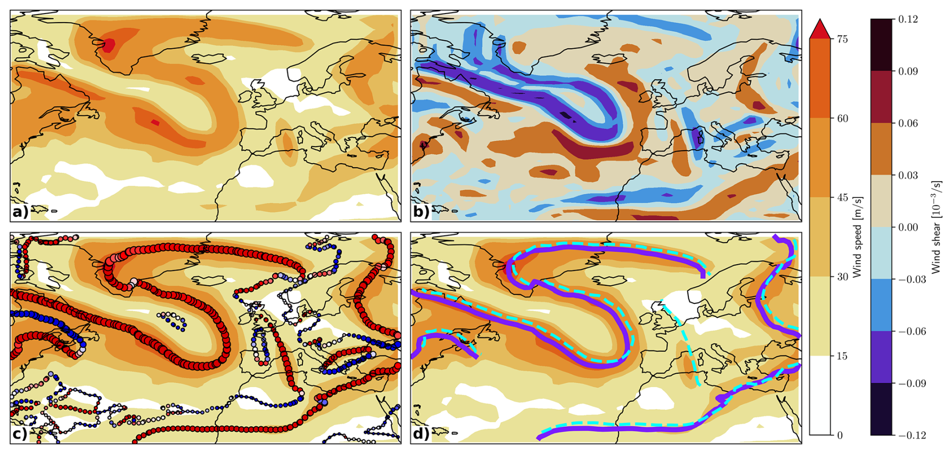
Figure 2 Results of our jet detection algorithm for 00:00 UTC on 9 October 1959. (a) The smoothed, vertical maximum wind speed [meters per second] field given as input to the algorithm. (b) The smoothed horizontal normal wind shear on the same 2D surface. (c) The τ = 0 contours where the size of the points corresponds to the wind speed field and the color corresponds to the alignment with the horizontal wind vector field from blue (close to −1) to red (close to +1). (d) The jets extracted from contours, as solid purple lines. The output of the S17 algorithm is represented as dashed cyan lines for comparison.

2.3.2 Jet properties

Introduced by Woollings et al. (2010), the Jet Latitude Index (JLI) measures the latitude of maximum wind speed in the profile obtained by averaging the wind speed field at low altitudes to filter out the STJ and only capture the EDJ, in a longitudinal band, originally 60° W–0° E, in the North Atlantic basin. It is often used in combination with the Jet Speed Index (JSI), the maximum wind speed used to find the JLI. These simple and highly interpretable metrics have been used to describe EDJ variability at timescales ranging from daily to multi-decadal (Woollings et al., 2014, 2018a).

Over time, several other similarly simple yet powerful jet indices have been developed to describe the jet stream in a simplified way or to link it to other phenomena. Such indices include the zonal jet index (Harnik et al., 2014), several sinuosity/waviness metrics (Francis and Vavrus, 2015; Di Capua and Coumou, 2016; Cattiaux et al., 2016; Röthlisberger et al., 2016a; Huang and Nakamura, 2016) linked to extreme events and persistence (Röthlisberger et al., 2016b; Martin and Norton, 2023), and a 10-index toolbox (Barriopedro et al., 2023) that has been used for skillful predictions of cold and hot spells in Europe (Maddison et al., 2023).

In the presence of several jets, many of these indices give an incomplete or improper picture. Using our jet core detection algorithm (Sect. 2.3.1), all the jet indices can be computed for each jet individually. The details of computations and potential differences with the original metrics are explained in the following paragraphs.

In the previous section, Sect. 2.3.1, we mentioned point-wise jet properties storing each point's position and wind speed. The mean of these point-wise jet properties constitutes the first jet properties we compute. The ones of interest correspond to the mean position of the jet. The properties mean_lon, mean_lat, and mean_lev are all computed as weighted averages of the longitude λ, the latitude ϕ, and the pressure level p, respectively, using the point-wise wind speed values $U_a^k$ as weights. In the spirit of the JLI, the maximum wind speed is found and stored as spe_star. The position on the long–lat plane of this maximum is stored as lon_star and lat_star.

A path integral of the wind speed along the jet core and using the haversine distance is performed and stored as jet_int. Explicitly, the integral ∫Uds is discretized using central finite differences and computed with a discretized approximation of

$$\mathrm{d}s=\mathrm{2}R\arcsin \sqrt{{\sin }^{\mathrm{2}}\left({\displaystyle \frac{\mathrm{d}\mathit{\varphi }}{\mathrm{2}}}\right)\cdot {\cos }^{\mathrm{2}}\left({\displaystyle \frac{\mathrm{d}\mathit{\lambda }}{\mathrm{2}}}\right)+{\cos }^{\mathrm{2}}\left(\mathit{\varphi }\right)\cdot {\sin }^{\mathrm{2}}\left({\displaystyle \frac{\mathrm{d}\mathit{\lambda }}{\mathrm{2}}}\right)},$$

with R = 6.378 × 10⁶ m being the radius of the Earth. This integral is performed once more over a smaller domain (λ > 10° W) and stored as int_over_europe.

To obtain the local width of the jet a at a point k along its core, normal segments are drawn in continuous space on either side of the jet core, of length 10° each (see Fig. 3). Along each segment, the wind speed is interpolated from the gridded wind speed field. For each segment, the haversine distance between the core and the first point to have a wind speed below $\mathrm{0.75}\times U_a^k$ represents the local width of the jet on this side, and the full local width is the sum of the local widths computed on either side. In some cases, only one segment can be drawn if the jet core is too close to a boundary. In this case, the local width is simply twice the width computed on the only valid side. The local widths $w_a^k$ are computed on every jet core point and then averaged, with $U_a^k$ as weights, to finally obtain the jet's mean width.

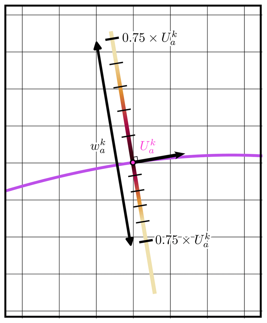
Figure 3 Schematic representing the local width computation, along a jet core a drawn in purple, for a single point k. In the schematic, the wind speed interpolated onto the half segments is represented using a color gradient from black (core wind speed at the point of interest, $U_a^k$) to yellow (three-quarters of local jet core wind speed, $\mathrm{0.75}\times U_a^k$) with a tick every $\mathrm{0.05}\times U_a^k$. The schematic, especially the grid spacing, is not to scale.

The tilt of the jet is computed as the slope of a $U_a^k$-weighted linear fit of the ${\mathit{\varphi }}_a^k$ against the ${\mathit{\lambda }}_a^k$. The linear coefficient is stored as tilt, while the intercept is discarded. The quality of this linear fit, the R² value, is used to compute a natural measure of jet waviness: waviness1 = 1−R². Another natural way of characterizing waviness from jet cores is the $U_a^k$-weighted average distance between ${\mathit{\varphi }}_a^k$ and mean_lat, stored as waviness2. For short jets, the difference between the tilt and the waviness is hard to assess, and in this case waviness1 will not capture waviness well. However, if a jet is both tilted and wavy, only waviness1 will be able to separate these properties. These two waviness metrics are compared against adaptations of waviness metrics found in the recent literature. wavinessFV15, adapted from Francis and Vavrus (2015), is computed as the $U_a^k$-weighted average of the local meridional circulation index: ${\text{MCI}}_a^k$ = $\frac{(v_a^k-\stackrel{\mathrm{‾}}{v_a})\left|v_a^k\right|}{(U_a^k{)}^{\mathrm{2}}}$. wavinessDC16, adapted from Di Capua and Coumou (2016), is computed as the ratio between the haversine-integrated length of the jet (∫1ds) and the length of the circle arc $\stackrel{\mathrm{‾}}{\mathit{\varphi }}\cdot R\cdot \mathrm{\Delta }{\mathit{\lambda }}_a$, where $\stackrel{\mathrm{‾}}{\mathit{\varphi }}$ is mean_lat and Δλ_a is the extent of the jet in longitude expressed in radians. Finally, wavinessR16, adapted from Röthlisberger et al. (2016a), is computed as the sum of absolute differences in latitudes between neighbors $|{\mathit{\varphi }}_a^{k+\mathrm{1}}-{\mathit{\varphi }}_a^k|$, divided by the sum of differences in longitudes.

An index that can be computed that will not be categorized per jet is the double-jet index. From the jets found, a 2D (time–longitude) binary array is built, where an element is set to True if at least two jets can be found at this time step and longitudinal band over all latitudes and one hemisphere. The index is the zonal average of this array for longitudes over Europe, 10° W < λ < 40° E.

In Sect. 2.3.4, tracking the jets allows us to determine the lifetime of a jet object, as well as the instantaneous speed of the jet's center of mass.

2.3.3 Jet categorization

While some literature sees the types of jets highlighted in the Introduction as regimes of a singular jet stream (Harnik et al., 2014, 2016), this work benefits from seeing them as categories one may assign to the previously detected jets. In instantaneous data, one cannot distinguish the jet from the eddies potentially driving it, since the quantification of the eddy momentum flux requires temporal filtering and averaging (e.g., Lachmy, 2022). One may instead rely on the vertical extent or baroclinicity of the jet, which is sometimes misleading due to the many factors influencing low-level winds; latitude, which is not sufficient on its own for global data (Winters and Martin, 2017); or potentially other metrics like vertical shear (Martius et al., 2010) or the height of the tropopause above the jet core. A recent, promising approach to establish this categorization bins the jets on the 2D feature space (wind speed–potential temperature). The algorithm then extracts regions of high occurrences for oceanic basins across the world and for the whole year. The approach always finds two distinct regions that may be labeled STJ and EDJ, except for the North Atlantic basin in JJA (Spensberger et al., 2023; see their Supplement for JJA).

A very similar approach is used here but with another feature space to better highlight the weak but still present bimodality in the jet property distribution in this basin and season. Our version of the algorithm uses the (baroclinicity–potential temperature) 2D phase space and fits a two-component Gaussian mixture model to facilitate the discovery of the two regions. The baroclinicity or vertical-extent proxy is similar to that used by Koch et al. (2006) and is defined as the ratio of low-level (500 hPa) horizontal wind speed magnitude at the horizontal position of the jet point to the jet core speed itself. An illustration of this binning can be seen in Fig. 4, where the count of jet points in each hexagonal bin is represented by its lightness and size.

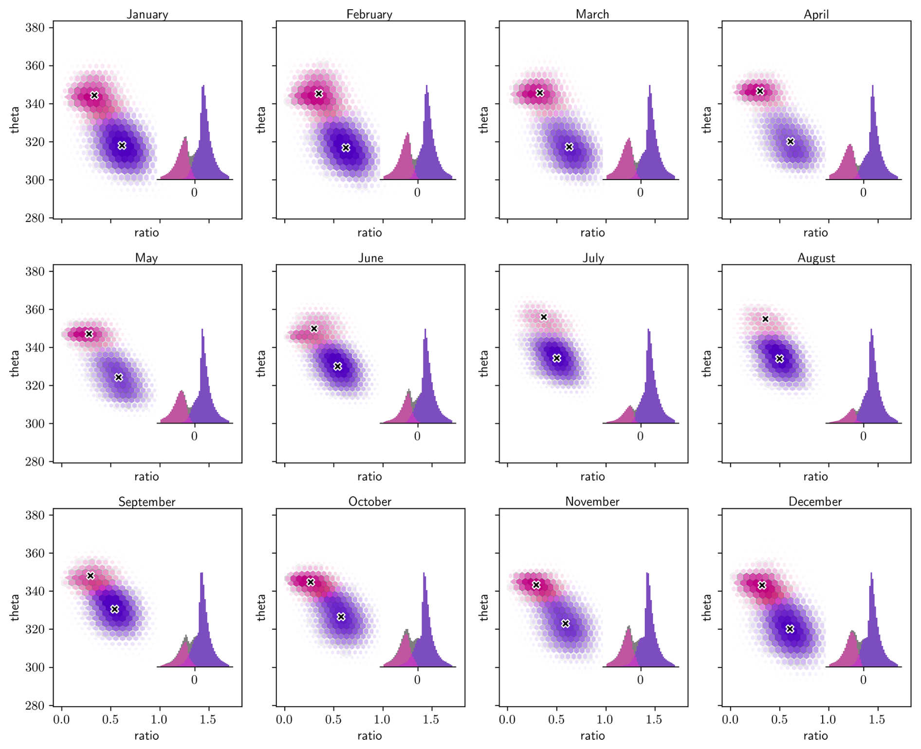
Figure 4 Demonstration of the jet categorization for each month of the year. The jet points are binned in the 2D space (baroclinicity proxy–potential temperature), in order to illustrate the underlying distribution in this 2D space. The size and lightness of each hexagon illustrate its height, while its color indicates the mean Gaussian assignment score, from pink (0 score, close to STJ component) to purple (1 score, close to EDJ component). The crosses indicate the center of each Gaussian, x₁ and x₂. In the lower-right corner of each box, the quantity $\log \frac{\Vert x-x_{\mathrm{1}}\Vert }{\Vert x-x_{\mathrm{2}}\Vert }$ is binned, where x is a 2D vector containing a jet point's vertical-extent proxy and potential temperature and $\Vert y\Vert$ is the 2-norm of the vector y. This quantity is not the final score but serves illustrative purposes. The final score is averaged for each bin and indicated with the color of each bar, as for the hexagons.

A two-component Gaussian mixture model assumes that the data are bimodal and tries to fit their empirical distribution as a sum of two Gaussian distributions. Each Gaussian is defined by a mean and covariance matrix that are fitted to the data. The model is fitted independently for each month to accommodate the large seasonal variation in the STJ's occurrence frequency. The density in the EDJ Gaussian component at each point, computed using the standardized distance to this component's center, is then used as a continuous score and not a hard assignment. The EDJ component is identified as the component with lower potential temperature. Most jet points will have a score close to 0 (STJ point) or close to 1 (EDJ point), but some points lie in between and can be thought of as hybrid. The jets as a whole are assigned a category based on the mean of the scores of the points that constitute them.

The nature of this potential hybrid jet category is discussed in Appendix A. In short, it has an almost identical seasonal cycle to that of the STJ and is almost only present in JJA. Our final decision was therefore to carry on with only two categories, with a categorization cutoff informed by the distribution of the EDJ component mean score.

2.3.4 Jet tracking

A straightforward object tracking algorithm is presented in this section. The program will assign a flag n to each jet at each time step, where the flag is carried over from a jet in a time step to a jet in the next one according to a distance threshold.

The algorithm starts by assigning each jet in the first time step a unique flag of $\mathrm{1},\mathrm{2},\mathrm{3}$, etc. It then iterates over all time steps t. For all flags that have appeared at least once in the previous four time steps (t−1, t−2, t−3, t−4, i.e., a day with a time resolution of 6 h), the algorithm extracts the most recent jet with this flag into a list of potential parents. This allows for jets to disappear for a few time steps and mitigates the issue of short jets blinking in and out of the jet integral threshold from Sect. 2.3.1. The potential children are all the jets present in the current time step. For all pairs of a potential parent jet a and a child jet b, an overlap measure o_a,b as well as a vertical distance δ_a,b is computed as described in Eqs. (3) and (4).

$$\begin{array}{}\text{(3)}& {\displaystyle }{o}_{a,b}={\displaystyle \frac{|{\mathrm{\Lambda }}_a\cap {\mathrm{\Lambda }}_b|}{\mathrm{2}}}\left({\displaystyle \frac{\mathrm{1}}{L_a}}+{\displaystyle \frac{\mathrm{1}}{L_b}}\right),\text{(4)}& {\displaystyle }{\mathit{\delta }}_{a,b}={\displaystyle \frac{\mathrm{1}}{|{\mathrm{\Lambda }}_a\cap {\mathrm{\Lambda }}_b|}}\sum _{k,l:{\mathit{\lambda }}_k={\mathit{\lambda }}_l}^{L_a,L_b}|{\mathit{\varphi }}_l-{\mathit{\varphi }}_l|,\end{array}$$

where Λ_a is the ensemble of longitudes in jet a.

Both overlap and vertical distance metrics need to satisfy a certain threshold, 0.5 and 10°, respectively. If both are met, the jets match and the child jet is assigned the parent's flag. If a child matches no potential parent, it is assigned a new flag, the latest assigned flag plus 1. If a child has two potential parents fulfilling both criteria or if a parent has two children fulfilling them, the winner is the most recent one, and if both are as recent, then the winner is the longest.

Using this, it is possible to infer the lifetime of a jet from its genesis to its decay, as well as track the speed of its center of mass (COM), in meters per second using the haversine distance between two 6-hourly time steps. The first use of these new jet properties is to filter out jets with 1- or 2-time-step lifetimes to filter out residual noise. The lifetime and (the inverse of the) COM speed can be seen as additional measures of persistence of the jet and can be compared against those developed within the framework of the SOM.

3 Results

3.1 Atlantic JJA SOM space

The results of the SOM training are summarized in Fig. 5 in a grid that represents its topology. Each panel is a wind speed composite of all time steps belonging to the corresponding cluster. The population of each cluster is shown in Fig. 6a. The jet finding and categorization algorithm is applied to these composites, and the results are overlaid with purple and pink lines for the EDJs and STJs, respectively. Since composites have lower wind speeds than instantaneous data, the point-wise wind speed threshold is lowered to 20 m s⁻¹ and the jet-wise integrated wind speed threshold to 3×10⁸ m² s⁻¹. Long jets that exhibit an EDJ region and an STJ region (see Sect. 2.3.1) are split into two automatically, on clusters 1 and 7, so that we can later on derive jet properties directly from the SOM composites, in Appendix C.

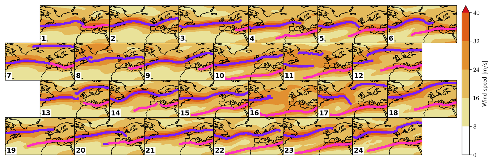
Figure 5 SOM training results on JJA wind speed fields. Composites of horizontal wind speed for all days corresponding to a cluster and results of the jet core detection algorithm applied to the composite wind fields overlaid as colored lines: pink for STJ and purple for EDJ. The SOM cluster number is indicated by a number in the bottom-left corner.

We first assess a few regions of interest in the SOM from a qualitative study of the composites. Clusters where both jets are present and overlap zonally (double jets) are located on the right side of the grid and in the bottom row. A subsection of this high-overlap region of the grid on the center-right columns, clusters 16, 17, 22, and 23, has the subtropical jet over the Sahara, while for most other clusters with double jets, the STJ is further north above the Mediterranean. The EDJ is especially wavy in clusters 2, 6, 9, 12, 13, 14, 17, 18, and 24. Clusters 11 and 16 contain more noisy and smaller-scale jet features than the rest of the SOM. In the composites of cluster 2, the region of high wind speed at the eastern edge that could be interpreted as an STJ is too weak and short in the domain to be captured by the jet detection algorithm.

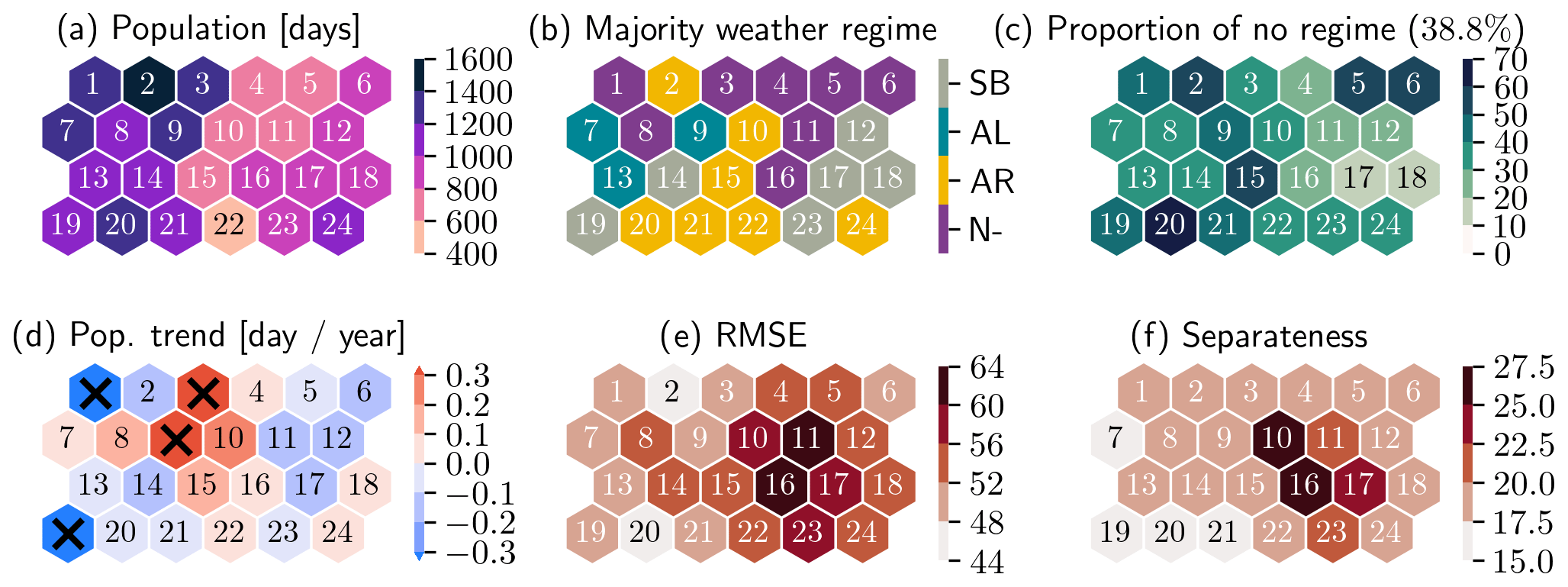
Figure 6 Climatological SOM cluster-wise properties. (a) Population, in number of days in JJA 1959 to 2022. (b) Weather regime with maximum occurrence frequency relative to each SOM cluster, excluding “no regime”. The shorthand terms correspond to NAO− (N−), Atlantic Ridge (AR), Atlantic Low (AL), and Scandinavian blocking (SB). (c) Proportion of time steps within each SOM cluster not associated with any weather regime, as in Grams et al. (2017), in percent. (d) Trends (1959–2022) in population in days per JJA. Significant trends at the 95th percentile are marked with black crosses. (e) Root mean square error of each cluster. (f) Separateness of each cluster, as defined in the main text.

Figure 6 shows six SOM cluster-wise properties using a hexagonal grid representing the SOM. The first property (panel a) is the cluster population. There is up to a factor of > 3 between the least and the most visited cluster, and the left side of the SOM, featuring shorter and weaker STJs, is a lot more represented than the right side. The least populated cluster, 22, corresponds to a south-shifted STJ with a wavy EDJ, while the most populated cluster, 2, features a strong, elongated, and wavy EDJ and does not feature a visible STJ.

The clusters are related to the summer Euro-Atlantic weather regimes (Fig. 6b and c) to simplify their interpretation and compare both approaches. This is done by calculating the weather regime occurrence probabilities conditional on each SOM cluster occupancy. The most represented weather regime in each SOM cluster, excluding “no regime”, is shown in panel (b), while the proportion of time steps during which a SOM cluster is occupied but no regime occurs is presented in panel (c). Clusters 18, 12, 17, and 14 are associated with the Scandinavian blocking regime, and the corresponding relative occurrence frequencies are the highest in all the cluster–regime pairs (not shown). This is probably due to the distinctive footprint blocking has on the jet, a large poleward shift of the EDJ above Europe. Interestingly, cluster 13, which has a very similar jet structure, is not as strongly linked to this regime but instead to the Atlantic Low regime, along with clusters 7 and 9. The NAO− regime is associated, as expected, with SOM clusters with a very zonal EDJ (1, 3, 4, 8, and 11), although the conditional probabilities remain low. The Atlantic Ridge is not strongly associated with any SOM cluster in particular, and no regime appears frequently in most SOM clusters, up to 70 % of the time.

In panel (d), interannual population trends are shown for all clusters. The most negative trend in population, cluster 1, corresponds to a zonal EDJ and a short, north-shifted STJ and is strongly associated with NAO− (panel b). The second most negative trend, cluster 19, features a zonal EDJ and weak, north-shifted and elongated STJ and is not strongly associated with any weather regime. The strongest positive trends (clusters 3 and 9) correspond to strong EDJ situations, one zonal (3) and one wavy (9), as well as weak and short STJs, without strong association with any weather regime.

We also provide two quality metrics for each SOM cluster: the associated RMSE (Fig. 6e), where a high value represents a cluster whose weight matrix is a poor representative of many of its members, and the separateness (Fig. 6f), where a low value represents a cluster whose weight matrix is very similar to that of its neighbors. We see hotspots in both RMSE and separateness for clusters 10, 11, 16, and 23. These clusters contain more diverse synoptic situations (high RMSE) than the other clusters and are different in their mean to the rest of the clusters, especially those close to them on the grid.

Next, we show the typical JJA pathway through the SOM in Fig. 7. This figure shows weekly binned cluster populations for all weeks of JJA and averaged over all JJA seasons for 1959 to 2022. It shows that a small subset of clusters in the center-right columns of the SOM represents most of the circulation during the first week of June, while clusters on other columns are much more likely to be visited in July and August, indicating a marked transition of the circulation patterns during June in the mean over all years. The shift from the center-right columns to the center-left and edge columns of the SOM grid at the end of June corresponds to a reduction in double-jet occurrence and an increase in mean STJ latitude, particularly in July and August.

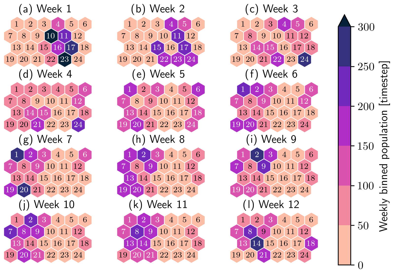
Figure 7 Weekly JJA pathway, the weekly binned cluster population for all weeks of JJA and averaged over all JJA periods. Week 1 corresponds to the first week of June and week 12 to the previous to last week of August.

The first week of June, which is climatologically different from the rest of JJA, has its variability almost entirely constrained to a few clusters, 10, 11, 16, 17, and 23 (Fig. 7). The RMSE on these clusters is higher than for the rest of the SOM (Fig. 6e). The clusters previously identified as early-June clusters are almost never populated again past 1 July. The clusters in the upper-left corner (1, 2, 3, 7, 8, and 9) are the most populated in late July and early August.

3.2 Jet stream properties

Using the detected and categorized jets, we study the properties of each jet category separately. We have defined numerous jet properties, and many of them are correlated with one another, so only a selection of six are shown in the main text, while results for a larger selection are presented in Appendix B.

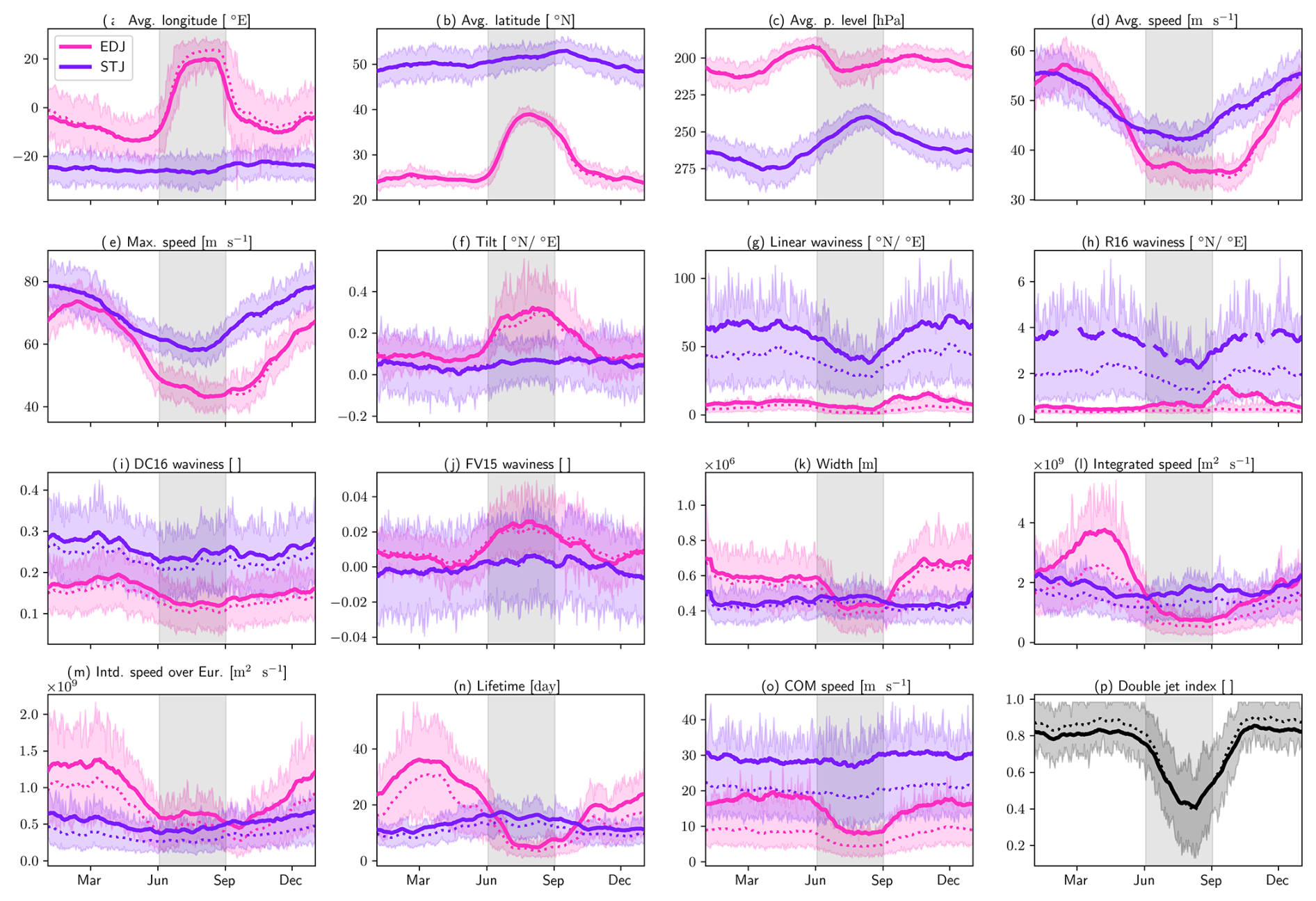
The six properties chosen have all seen keen interest in the literature. The average latitude can be compared to the JLI (Woollings et al., 2010), while the max speed can be compared to the JSI or to the 99th percentile of wind speed (Shaw and Miyawaki, 2024). The (inverse of the) jet's COM speed can be viewed as a proxy for persistence. The waviness, as defined by Di Capua and Coumou (2016) and hereafter named DC16 waviness, is a simple metric to quantify the departure from zonality of the detected jets. The width of the jet has been emerging as another feature of interest in the recent literature (Peings et al., 2018) and is here computed using natural coordinates. Finally, we determine, at each longitude, whether both jets are present and average this overlap Boolean quantity over the European sector (λ > 10° W). The mean latitude, max speed, and width distributions have low skew, while the COM speed, waviness, and double-jet index's distributions are very skewed with tall peaks at low values and long tails.

The seasonal variability of this selection of jet properties is presented in Fig. 8. Several interesting features can be observed in this figure. First, the month of June is once more highlighted as a transition month that is different from the rest of JJA. More precisely, the speed of both jets and the waviness of the STJ reduce in the months leading up to June (Fig. 8b and d). Then, during June, both jets move poleward, with a much more pronounced shift for the STJ (Fig. 8a).

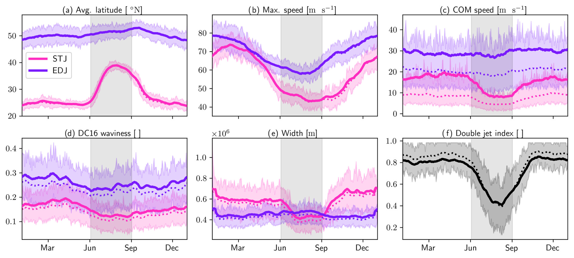
Figure 8 Euro-Atlantic jet property seasonal variability. The results are split by jet category and always colored in the same way: pink for the STJ and purple for the EDJ. The double-jet index is colored in shades of gray. A 15 d window averaging is applied to the day-of-year mean (thick line) as well as the day-of-year median (thin dotted line) but not to the inter-quartile range (shading). The marker label for each month corresponds to the first day of this month. The gray rectangle in the middle of each panel represents JJA.

The seasonal variability in latitude and the seasonal variability in speed of the EDJ are very comparable to the Jet Latitude Index and Jet Speed Index seasonal variabilities (Woollings et al., 2014) and the storm track seasonal variabilities (Hoskins and Hodges, 2019) for the equivalent EDJ properties (average latitude and max speed, respectively). The amplitude and width of the JJA peak in STJ latitude can be compared with those in Maher et al. (2020). Seasonally, the STJ follows the expansion and weakening of the Hadley cell in the Northern Hemisphere summer (Dima and Wallace, 2003; Davis and Rosenlof, 2012).

In contrast, the speed of the COM, the DC16 waviness and the width do not show strong seasonal variabilities (Fig. 8c, d, and e), with signals staying well below the interannual variability, with the exception of the STJ's waviness, which shows a peak in spring and a slight dip in EDJ width in summer compared to winter. The jets are much closer together in JJA than the rest of the year but overlap less often, mainly due to the subtropical jet occurring less often in JJA (see Fig. 4).

An important question is how these properties have evolved under past climate change. Figure 9 shows the interannual JJA trends for the six selected properties. Statistical significance is tested using block bootstrapping, with 10 000 bootstrapped time series created with a block size of 4 years.

Trends in JJA are yet to emerge out of the interannual variability, as only 3 of the 11 trends shown in Fig. 9 are significant, a negative trend in the max wind speed of the STJ and a positive trend in the waviness of both jets with the DC16 definition. The STJ max wind speed trend is consistent with the findings of D'Andrea et al. (2024), who report a significant decrease in zonal wind of between −0.1 and −0.5 m s⁻¹ per decade in the area corresponding to the location of the STJ in JJA (see Fig. 5). The trends in waviness, while large in this figure, are dependent on the definition, as we showcase in Appendix B. An increase in waviness in this region is consistent with, e.g., Francis and Vavrus (2015) and Cattiaux et al. (2016). It is also consistent with a positive trend in occurrence frequencies for SOM clusters featuring wavy or tilted (3, 9) and negative trends in clusters presenting more zonal jets (1 and 19). It is worth mentioning that, with our definition, there is only a non-significant negative trend in double-jet index in this domain.

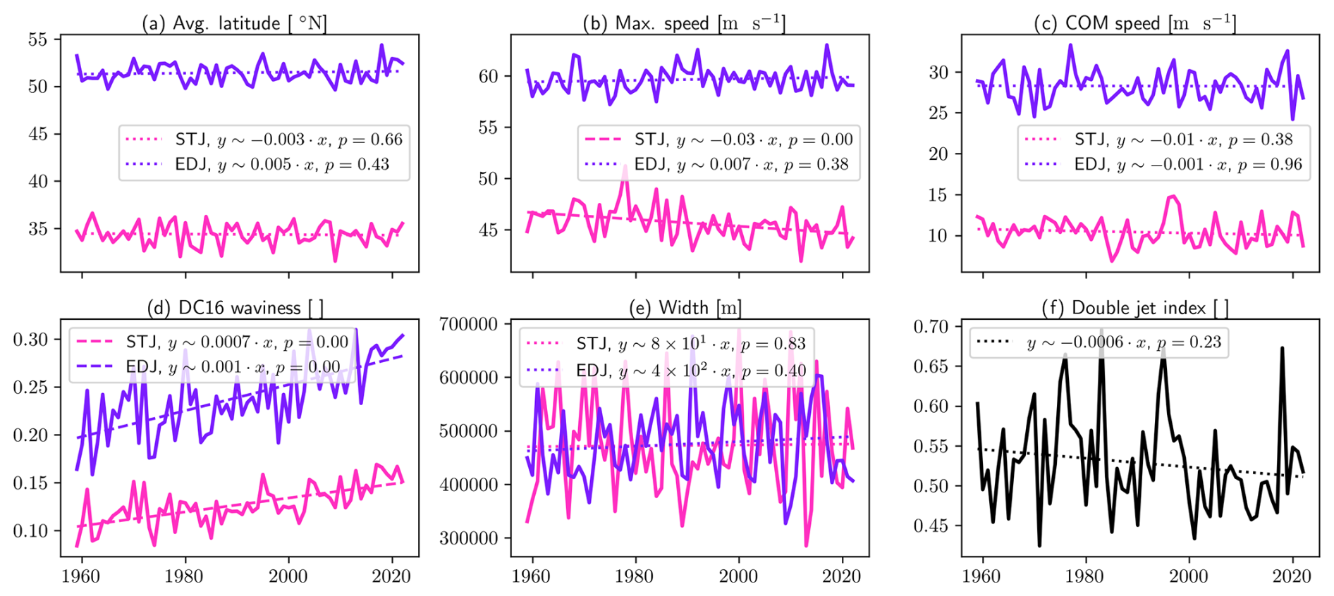
Figure 9 Euro-Atlantic jet property JJA means and interannual trends, split by jet category. Linear trends represented by dashed lines are significant at the 95th percentile, while the dotted lines are not.

Trends of these six jet properties can be viewed at a finer temporal scale, for each day of the year, in Fig. 10. The significance is once more established using block bootstrapping with the same settings as for Fig. 9, and it is assessed prior to the 60 d rolling-window smoothing.

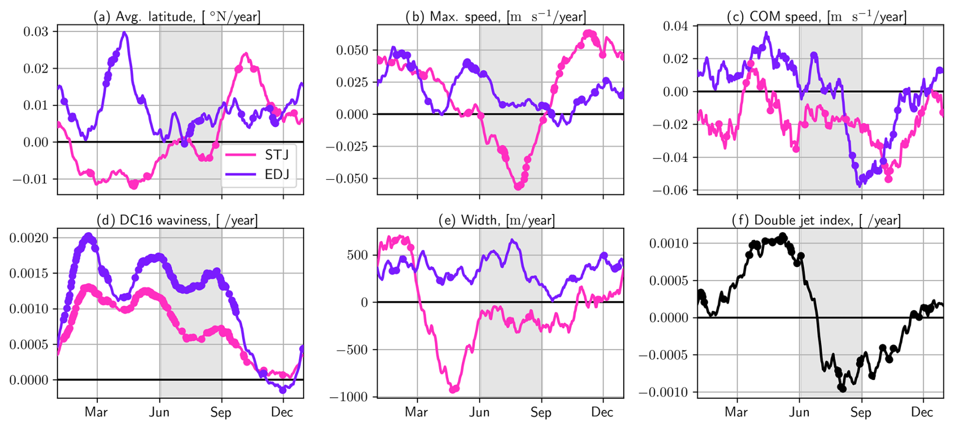
Figure 10 Euro-Atlantic jet property interannual trends, computed independently for each day of the year, and the result smoothed by a 60 d rolling window. Trends significant at the 95th percentile are marked with a thick dot. Significance is assessed prior to smoothing.

The EDJ exhibits a poleward shift across most seasons, consistent with the arguments of Held (1993) (Fig. 10a). The STJ shows an equatorward trend in spring and a poleward trend in autumn (Fig. 10a). The EDJ maximum wind speed increases consistently across the whole year, with the strongest of intensification in February, March, May, and June (Fig. 10b). This result can be linked to results in past data (Woollings et al., 2018a; Harvey et al., 2023) and in future simulations (Shaw and Miyawaki, 2024). The STJ has opposite trends in its max speed between JJA, where the trend is negative, and September to December, where the trend is positive (Fig. 10b). No strong trends appear in our results for the COM speed, except a negative trend in COM speed in July and August for the EDJ and in September and October for the STJ (Fig. 10c). DC16 waviness increases significantly, for both jets and consistently over the whole year, with a stronger increase between January and June (Fig. 10d), which is mostly consistent with, e.g., Cattiaux et al. (2016) and Di Capua and Coumou (2016), albeit in different regions. The width does not show strong trends except a negative trend in April and May for the STJ (Fig. 10e). Finally, the double-jet index increases significantly in March, April, and May and decreases significantly in July and August (Fig. 10f), although the trends in JJA averages were not significant (Fig. 9).

3.3 Jet properties on the SOM

In this section, we make use of the detected jets and their properties to assess the capabilities of the SOM to capture jet stream variability as opposed to random noise. First, we composite jet core detection probability, separated by jet category, and overlay the jet cores found in the SOM wind speed composites, i.e., Fig. 5. The results, visible in Fig. 11, show clear agreement on the position of the detected jet cores as well as on their categorization.

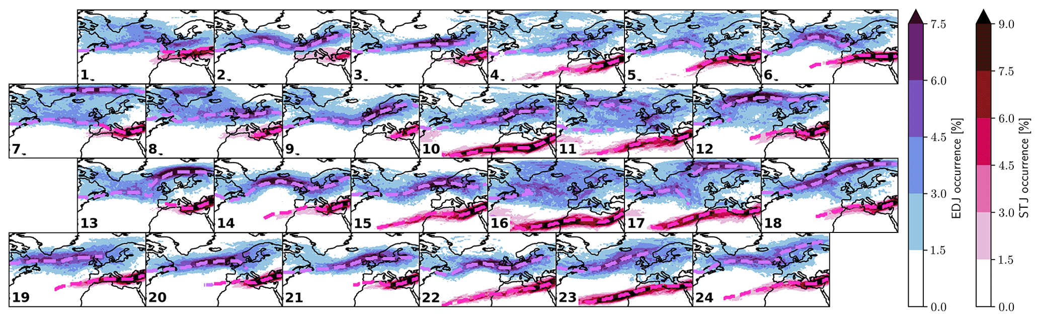
Figure 11 Jet core detection probability composites (blue shading for EDJ, pink shading for STJ) and jet cores found in wind speed composites, Fig. 5, as colored lines (purple for EDJ, pink for STJ).

As a way to compare and validate the results of both methods, a selection of jet properties are projected onto the SOM clusters, shown in Fig. 12.

The latitude of the EDJ is, as in the composites, higher in the extremal columns than in the central columns of the SOM (panel a), and the clusters with the highest mean EDJ latitude also correspond to clusters with high relative occurrence of the Scandinavian blocking weather regime (see Fig. 6b). The maximum speed of the EDJ is highest in clusters 10, 14, and 23. These three clusters have the highest population during the first (10 and 23) or the last (14) week of JJA (see Fig. 7), when the EDJ has the highest max speed in JJA (see Fig. 8). Similarly, the EDJ max speed is lowest in clusters populated in the middle of JJA (clusters 1, 7, 12, 19, 20). The EDJ waviness is highest in most clusters associated with the Scandinavian blocking or Atlantic Low regimes and lowest for clusters associated with the NAO− or Atlantic Ridge regimes, with the notable exception of cluster 8, weakly associated with NAO− but very wavy (see Fig. 6b, relative occurrence not shown).

The double-jet index, as well as the max speed, mean latitude, and width of the subtropical jet, follows the very clear seasonal signals presented in the previous section (Fig. 8) when matched with the weekly cluster populations (Fig. 7). The observations are also very consistent with what can be seen in the jet core probability composites (Fig. 11).

The observations made, qualitatively, from the wind speed composites (Fig. 5), can all be matched with the jets' mean properties on the clusters (Fig. 12). This result is not entirely trivial. It means that, for most clusters, the jets found in the cluster mean wind speed composites have properties corresponding to the mean of the properties of the jets found in each individual time step belonging to that cluster. In other words, the wind composites and the jets found therein are representative of the wind speed snapshots, as well as their jets, belonging to each cluster and not merely artifacts of averaging noisy fields. These observations are quantified in Appendix C.

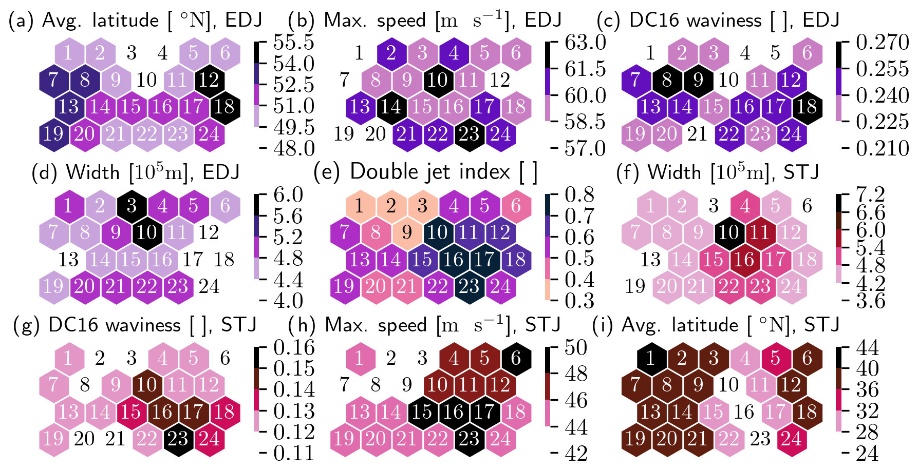
Figure 12 Jet properties, separated by jet category when applicable, projected onto the SOM clusters. Shades of purple correspond to EDJ properties and shades of pink to STJ.

3.4 Jet persistence

We characterize persistence using three metrics extracted from the residence times for each SOM cluster and two metrics for each jet category, the jet lifetime and the speed of the center of mass. To compare all of these metrics, we aggregate their results for each SOM cluster and plot the results in a hexagonal plot as in Sect. 3.3.

Our definition of residence times allow for departures one cluster away from the origin cluster (see Sect. 2.2.3). We first count the number of stays that last more than 4 d on each SOM cluster (Fig. 13a). The lengths of stays of any length are aggregated as JJA averages (panel b) and 95th percentiles (panel c). The summer averages give an approximation of the state persistence (Tuel and Martius, 2023), i.e., an estimate of how much time the large-scale circulation pattern typically needs to move from one state into the next, while the number of long stays and the 95th percentile of residence times capture more episodic persistence, i.e., the most persistent events of each flow configuration.

Clusters 1, 2, 3, and 20 are characterized by a large number of long stays and a high state and episodic persistence. These clusters all represent a roughly similar synoptic situation of a zonal EDJ extending over the British Isles and with slightly positive tilt but with minute differences in the apparent EDJ waviness and length of the STJ. These are very well defined clusters (low RMSE) but with the lowest separateness in the SOM, which confirms our observations from their composites. In the rest of the SOM, the state persistence and episodic persistence seem to be correlated, and the previously highlighted region of clusters representing the first week of June (10, 11, 16, 17, and 23) does not stand out as more or less persistent than the clusters representing the rest of JJA.

Results from the projection of jet-wise persistence metrics onto the SOM show mixed agreement with the SOM persistence metrics, at least in this presentation of temporal aggregates, as well as mixed agreement among each other. High COM speeds of either jet, which indicate low instantaneous persistence, can be associated with either low or high state persistence and with either a low or a high jet lifetime, for jets of the same or a different nature. It is worth remembering that, while all of these numbers characterize persistence in some sense, they are very different in nature. Jet lifetime and SOM average residence time are both nonlocal, which means they can only be determined when a jet has weakened below the jet integral threshold or left the domain and when a stay on a SOM cluster has ended. Additionally, the two jet-related metrics only assess the persistence of one jet at a time, which can be very different. This can make these metrics unfit to qualify a time step or a period concisely.

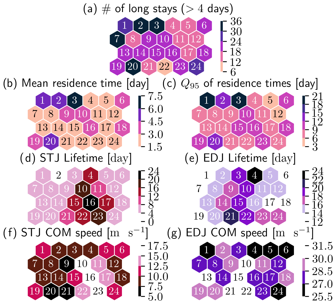
Figure 13 Persistence properties of the SOM clusters. (a) Number of long stays on each SOM cluster. (b) Mean residence time on each SOM cluster. (c) The 95th percentile of residence times on each SOM cluster. The definition of residence time here is loosened to allow for a stay to be unbroken as long as the jumps are to a cluster similar enough to the starting cluster (below the 10th percentile of pairwise distances between cluster weight matrices). (d–g) Jet persistence properties, separated by jet category when applicable, projected onto the SOM. Shades of purple correspond to EDJ properties and shades of pink to STJ.

4 Discussion and summary

We use two complementary methods, self-organizing-maps (SOM) and jet core detection, to characterize the upper-level tropospheric jets and apply them to the Euro-Atlantic sector in the less studied Northern Hemisphere summer season, along with some year-round results. The SOM method specializes in finding dynamical properties of the overall flow, including persistence, while the jet core detection method finds properties of individual jet cores at individual time steps, and we present for each the ERA5 interannual trend and intra-seasonal variability. These methods have overlap: for example the SOM shows a clear intra-seasonal variation in cluster population, and some of the jet properties are proxies for persistence. These overlaps allow us to verify the results between methods, increasing our confidence in our results.

The SOM, a clustering method with distance-preserving properties, allows us to study the circulation time series as a sequence of stays on a cluster and jumps between clusters, where the magnitude of the jumps is meaningful. A group of clusters with a low population, high mean cluster error, high cluster separateness, and a south-shifted STJ compared to the other clusters is shown to be comprised almost entirely of time steps in the first 1 or 2 weeks of June every year. This time of the year is therefore identified as having a very different mean synoptic situation to the rest of JJA, but its relatively low weight in the data compels the training algorithm to only assign a few clusters to it, too few to correctly capture the variability of this period.

The SOM is related to weather regimes using relative occurrence frequencies. With strict conditions for regime occurrence, a high proportion of JJA days is not assigned to any regime, and only a few SOM clusters can be strongly associated with weather regimes, typically to the blocking regime which is accompanied by a poleward shift of the EDJ above Europe, easily captured by our wind-based clustering approach.

Long stays on a SOM node is a natural way to evaluate state persistence. The most persistent clusters correspond to long EDJs that extend over the British Isles, and north-shifted, short, and weak STJs over the Mediterranean. Aside from those rough similarities, they present differences in EDJ waviness and maximum speed according to the mean jet properties projected onto the SOM. These clusters, which have high occurrence probability and persistence, typically do not project well onto any weather regime. There is a strong incentive to consider using more clusters than four, irrespective of the clustering method employed, when it is compatible with the research question. In this study, the larger number of clusters has allowed us to describe the majority of JJA time steps as cluster visits with low projection error and has all but guaranteed that all the persistent episodes can be extracted as long stays on SOM nodes, with our definition.

A variation of the jet core detection algorithm presented by Spensberger et al. (2017) is used to identify instantaneous jets and extract properties for each of them separately. The jets are classified into the two canonical jet categories (subtropical and eddy-driven jet – STJ and EDJ, respectively) and tracked over time to obtain metrics that offer another view of persistence. Once more, past trends and seasonal signals are extracted.

In JJA, the only significant trends are an increase in the DC16 waviness of both jets and a slowdown of the STJ. The poleward shift of the EDJ projected in, e.g., Held (1993) is not significant in our analyses in JJA, nor is the equatorward trend of the STJ reported by Totz et al. (2018). The absence of a trend in STJ latitude, seemingly at odds with the measured tropical expansion (e.g., Davis and Rosenlof, 2012), is consistent with findings in the recent literature (Davis and Birner, 2017; Maher et al., 2020).

Year-to-year trends, computed independently for every calendar day, vary a lot over the year at subseasonal timescales. The trends in 3-monthly averages that are often presented in literature can therefore sometimes be misleading, as they can average out strong trends of opposite signs. As an example, the double-jet index has a strong positive trend before and up to June and a strong negative trend in July, August, and September, so its trend in JJA average is weakly positive. Still, it is useful to continue discussing these trends in seasonal averages to create points of comparison with the past literature and because they allow us to illustrate the different amounts of interannual variability between jet properties.

Comparing results from the two methods, SOM and properties of the detected jet cores, helps to validate them. The SOM is shown to capture jets and not random noise because the jet cores detected in the composited wind fields match the probabilities of jet core detection, composited for every cluster, very well. The expert-defined jet properties succeed in characterizing features which dominate the leading patterns in the more statistical SOM approach. Computing properties of the jets at every time step before averaging them based on cluster membership gives very qualitatively similar results to computing jet properties on the jet cores extracted from each cluster wind speed composite, but the match is not perfect. Furthermore, the strong regime shift that happens in June, characterized most clearly by a weakening and poleward shift of the STJ, is distinctly picked up by both methods. Trends in waviness can be matched to positive trends in clusters with wavy or tilted jets. As a more subtle point, clusters that represent early June and have the highest mean double-jet index within this subset get more frequent, albeit weakly, than the rest of this early-June subset, while the opposite is true for the July–August subset of SOM clusters, which matches the opposite-sign trends in the double-jet index between early and late Northern Hemisphere summer well. This indicates that both methods are mostly coherent with one another.

The persistence metrics developed around the jet detection method show another facet of persistence in addition to the one expressed by the SOM cluster residence time, and the results of both methods often disagree. This is partly explained by their many differences in nature. Only the jets' COM speeds can be assessed locally in time, and the jet-related metrics only refer to persistence of a single object at a time, different from the state or episodic persistence quantified by SOM residence times.

The jet detection algorithm is directly applicable to global data, as are the jet property computation and the jet tracking. Global jet categorization would, however, have to use an adapted set of jet properties to distinguish the EDJ from the STJ, as longitude and latitude are only good discriminants in the Atlantic basin. A different set of jet properties might have to be used for each season or even each month, as the seasonal signals suggest. The SOM, like all clustering metrics, is not well suited for a global application and works best when restricted to a single basin. The steep increase in dimensionality and variability that accompanies an expansion to a larger region, combined with the same proportionally small number of time steps, creates a much more ill-defined clustering problem. Since both methods are relatively cheap computationally, they can be applied to large ensembles and higher-resolution model data to evaluate future trends and shifts in seasonal signal or persistence and predictability properties.

In future work, we will use these diagnostic tools to study the circulation before and during extreme weather events in Europe. Potential applications currently explored include assessing atmospheric persistence and predictability properties in the days leading up heatwaves, finding SOM clusters most likely to see the onset of a damaging hail storm, and discovering which jet properties can be used as good predictors for extreme surface winds in a statistical model.

The previous paragraph pertains to the jet stream as a potential driver of weather predictability, even if the causality can go in both directions. Another use for the methods is the investigation of the drivers of jet stream variability, for example, large-scale teleconnections like ENSO or local mechanisms like diabatic heating, as has been studied recently by Auestad et al. (2024). Another avenue is the exploration of the jets' tight relationship to Rossby waves, for example by assessing the ability of the detected jets to carry and guide Rossby waves (Martius et al., 2010; Wirth, 2020; Wirth and Polster, 2021; Bukenberger et al., 2023; White and Mareshet Admasu, 2025). Similarly, it is now easier to examine their relationship to Rossby wave breaking, for instance as triggers of large jumps in SOM clusters (Michel and Rivière, 2011) or as drivers of abrupt changes in jet strength, latitude, or center-of-mass speed (Martius and Rivière, 2016). Adapting the jet width method to instead find wave-breaking events around the jet core is showing promising early results.

Appendix A: Further exploration in jet categorization

In Fig. A1, we explore the effects of changing the categorization method on the seasonal variabilities of the categorized jet properties. First, in the first three rows of the figure, we vary the cutoff between STJ and EDJ. The effects on the mean position (in latitude and pressure level) are barely distinguishable, but the effects on the number of jets of each category per time step can be markedly altered by this choice, especially for the STJ when changing the cutoff from 0.1 to 0.5.

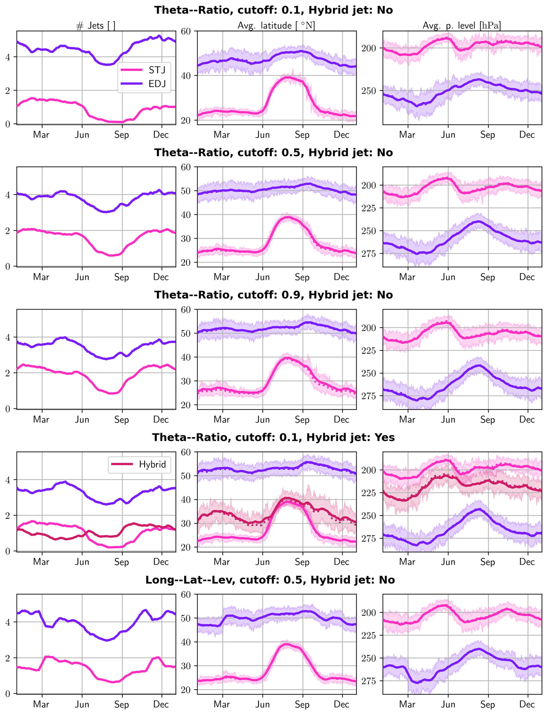
Figure A1 Seasonal variabilities of categorized jet properties with variations in the categorization method.

Then, we allow jets whose categorization score is between 0.1 and 0.9 to be assigned to the hybrid category. The aggregated properties for the three jets can be seen in the fourth row of Fig. A1. As many jets belong to the hybrid category as to the STJ in winter, while in JJA there are more hybrid jets than there are for the STJ, according to this cutoff. However, this hybrid jet has an almost identical seasonal cycle to that of the STJ, not only in its spatial distribution but also in its other properties (not shown). We therefore decided against introducing this third category in the paper, since it seems to behave like an STJ. This is also why we choose a cutoff of 0.9 in the main text. This way the STJ corresponds to well-defined STJs as well as to hybrid jets which we identify as worse-defined STJs.

We would interpret these findings as follows. In JJA, the subtropical jet is shifted north with the Hadley cell and interacts with extratropical eddies more, making it lose more momentum (Martius, 2014) and potentially making it more baroclinic. This makes the distinction more fuzzy, so there are more jets that do not fall cleanly onto either Gaussian, i.e., more jets with a score very different from either 0 or 1. These jets still seem to behave more like STJs than EDJs, potentially because most of their momentum still comes from the (sub)tropics and is conserved.

For comparison with our earlier categorization method that used only spatial information (longitude, latitude, and pressure level of the jet point), we perform the categorization one last time with this choice of discriminant variables. The results can be seen in the fifth and last row of Fig. A1 and are again similar. This previous method worked well in the North Atlantic basin but was not based on physical bases and did not generalize well to other basins. Both of those concerns are solved with the new method, which can be applied to hemisphere-spanning jets without modification.

Appendix B: Extended jet properties

In the main text, we highlight how many jet properties undergo a transition around the month of June, setting this month apart from the rest of JJA in terms of absolute values of these jet properties.

In order to give a more complete overview of the jet properties, we show the seasonal cycle of the complete set in Fig. B1.

Figure B1 Reproduction of Fig. 8 with a larger selection of jet properties.

Comparing the jet core's mean and max speeds shows little difference between the two in their seasonal cycles. The max speed trends are stronger as expected, but they also seem statistically more robust than mean core speed trends. The waviness metrics all show a different seasonal cycle, and they even disagree on which jet category is wavier than the other. Apart from the differences in the original metrics, this discrepancy can also come from how they were adapted to function on jets and more specifically the normalization factor used in several waviness metrics ($\mathrm{1}/\mathrm{\Delta }\mathit{\lambda }$) that favors high values for the STJ, which is typically much shorter in this domain. Another issue is that most of these metrics, from their definition, fail to distinguish small-synoptic-scale waviness and tilt. Only our linear waviness is designed to fully separate the two, but proposing another waviness metric is not our goal with this study. FV15 waviness is very close to our definition of tilt, and the seasonal signals of these two metrics are very similar. R16 waviness and linear waviness show an almost identical seasonal cycle too, despite the fact that, from their definitions, one could predict a very different behavior. Following on from our previous comments, it is not surprising that all of the waviness metrics show vastly different trends throughout the year (Fig. B2).

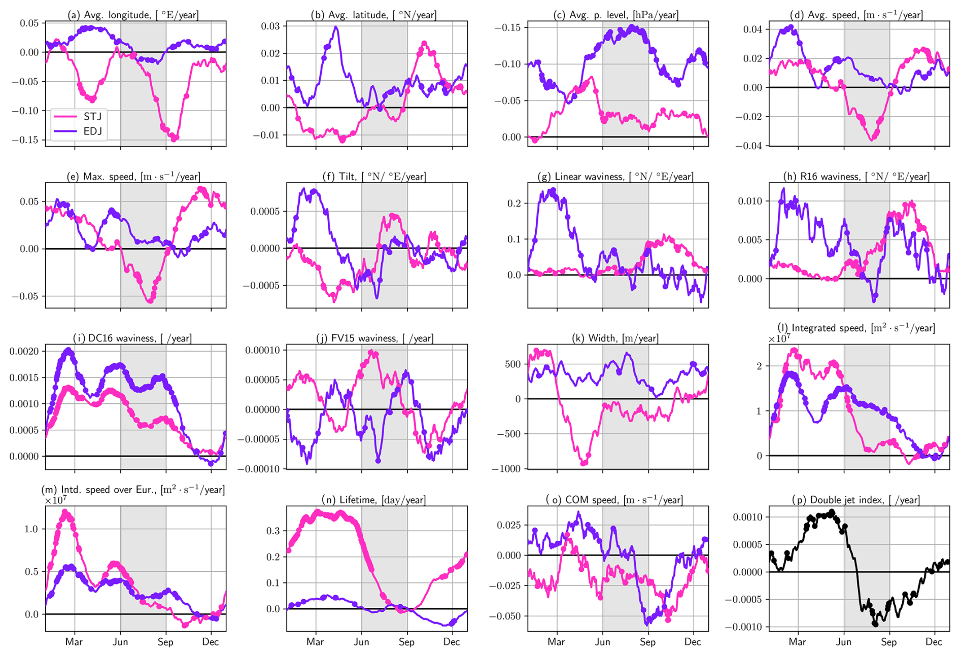
Figure B2 The 1959–2022 day-of-year interannual trends, smoothed using 60 d rolling-window averaging. Colored points indicate a significant trend at the 95th percentile.

Appendix C: Properties of the jets detected on SOM composites

In this appendix, we validate observations made in the main text about the capacity of SOMs to correctly capture the jet properties. We do so by measuring the properties of the jets detected in the wind field composites of Fig. 5. The results, shown in Fig. C1, point towards overall agreement with some caveats. First, the STJ is not detected in the composite for cluster 2, even though it is present in some time steps belonging to this cluster. Wind speed composites also have lower wind speeds than instantaneous fields overall, so the maximum speeds of both jet categories are reduced by about 10 m s⁻¹. If the absolute values cannot always be meaningfully compared between Figs. 12 and C1, the distribution of lower and higher values on the SOM can, and in this view there is large agreement.

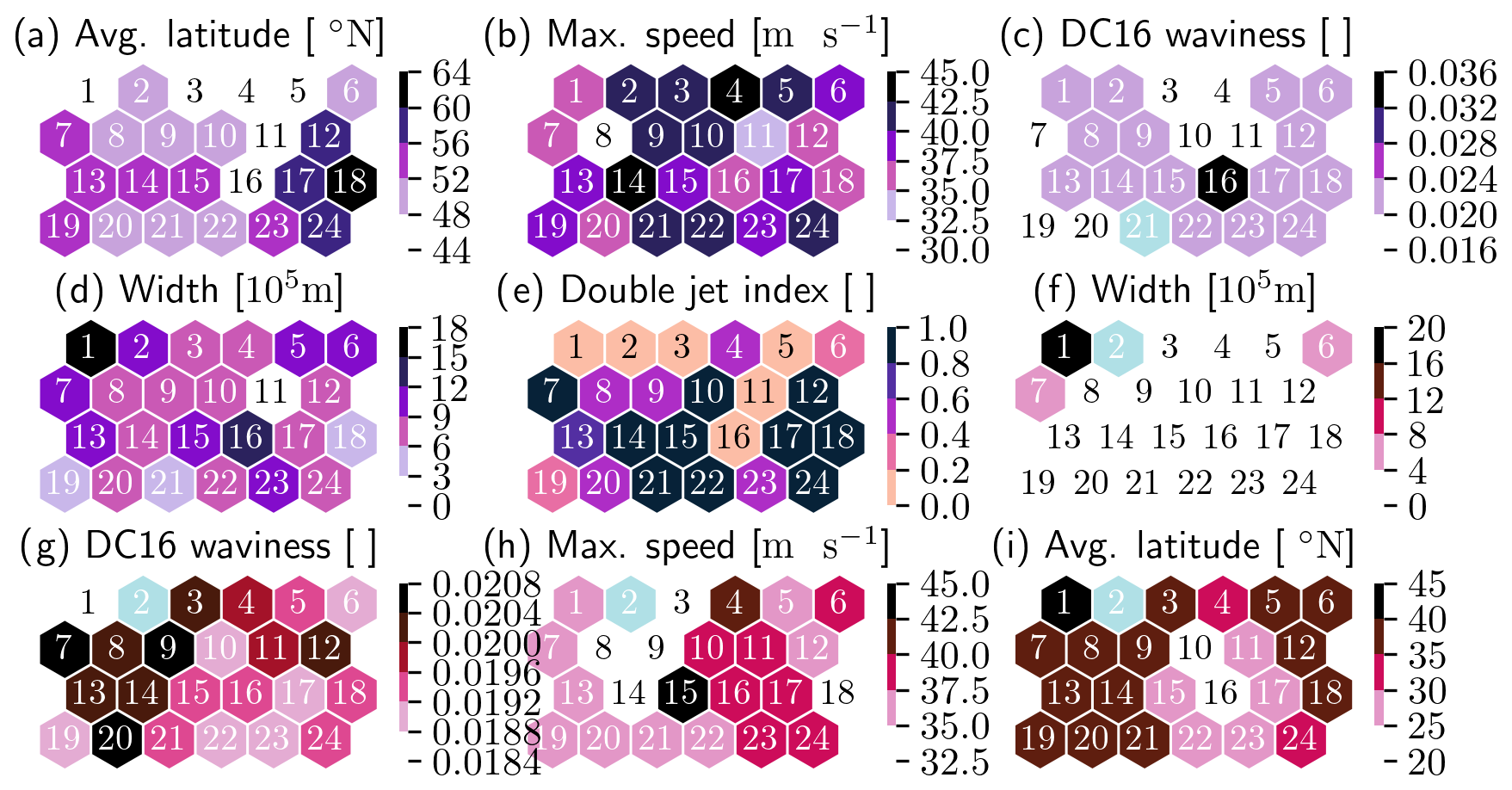
Figure C1 Jet properties, separated by jet category when applicable, computed from the jets detected on the SOM cluster centers. Shades of purple correspond to EDJ properties and shades of pink to STJ.

Appendix D: Overview of previously tried methods for jet core extraction

During the development of the jet core extraction algorithm, several different avenues were explored to improve its robustness or the execution speed and later abandoned in favor of the final version of the algorithm presented in the main text. We believe it is valuable to present negative results, both because these methods could be improved and used again in other relate applications and simply for future researchers in this field not to repeat methods that were explored but ultimately failed at improving the algorithm.

The first-version algorithm was an adaptation of the Koch et al. (2006) algorithm, also used in Pena-Ortiz et al. (2013). This algorithm uses a peak-finding algorithm on each latitude band before connecting the points longitudinally based on a distance criterion. The peak-finding algorithm requires several thresholds, and their tuning is challenging without an objective quality metric to grade the performance of the algorithm. More fundamental problems appear with forked jets, seen in SOM cluster 17 for instance.

The second version divides the task in two. First, potential jet regions are found using a relatively low wind speed threshold that can be made to be seasonally varying or even a quantile threshold to work well in all seasons. The regions are separated from each other using spatial agglomerative clustering. The second step of the algorithm is heavily inspired by Molnos et al. (2017). Each potential jet region is turned into a graph, with each grid point a node and edges connecting all of the nodes. The edges are assigned a weight based on the wind speed of the nodes/grid points they connect and on their alignment with the directional wind field (similarly to the current algorithm). From potential jets, the jet cores are found using a weighted shortest-path algorithm.

The difficulty of this second method comes from jet regions connecting to each other if they are too close and from the problem of determining start and end points of jet cores within the jet, with potentially several starts and ends within each potential jet region because of the first problem. Several avenues were explored to mitigate the first problem, which in turn made the second problem easier to solve, most notably, the use of computed vision techniques like thinning, skeletonization, and Sato filtering (Sato et al., 1998). This latter technique is used in medical imaging to highlight vessel-like structures in black-and-white images like blood vessels in biological tissue, and it seems very promising to help in jet detection. However, it also requires careful setting of its parameters, most crucially its filtering scales, which loosely correspond to the expected width of the jet in pixels. Solving these problems made the algorithm grow in complexity and computing requirements for few added benefits. This approach as well as other related ones was finally abandoned in favor of the simpler, more robust one presented in the main text.