Revisiting barotropic instability from the perspective of wave evolution theory

The instability of Rossby waves has been a long–standing topic in dynamical meteorology. The classic theoretical analysis had provided in–depth physical understanding of the problem. However, developing a systematic and quantitative comprehension of wave energy and amplitude evolution remains challenging. With an eye to such issues, this investigation provides a novel and practicable algorithm to solve the wave action conservation equation. Theoretical analysis establishs that wave packet energy evolves through two competing factors: direct proportionality to intrinsic frequency and inverse proportionality to group velocity magnitude. Energy density attains extremal values at turning points where group velocity magnitudes become extremized. To ensure a ray can be reflected by a turning point, zonal phase speed must be smaller than an upper limit determined by the dispersion relation at the turning point. Crucially, a specific zonal phase speed range emerges below this maximum threshold where concurrent transient growth of both wave energy and amplitude occurs when a ray is moving toward the turning point, with the upper limit corresponding to optimal wave development conditions. Numerical experiments on a prototype westerly jet reveal distinct instability mechanisms: substantial transient growth – capable of triggering nonmodal instability – arises when rays moves toward turning points, while exponential amplification characteristic of modal instability develops at inflection points with positive energy growth rate. The derived zonal phase speed thresholds and transient growth metrics form a diagnostic framework applicable to observed atmospheric flows, enabling quantitative evaluation of both modal and nonmodal instability potentials. By unifying wave evolution dynamics with classical instability criteria, this work provides an operational bridge between theoretical predictions and real–world flow diagnostics.

1 Introduction

Rossby waves are among the most fundamental dynamical features in the upper atmosphere. A key characteristic of Rossby waves, which has profound implications for their modulation of weather systems, is their propagation (Segalini et al., 2024). Accompanied by transfers of heat, moisture, and momentum in propagation and amplification, they play critical roles in shaping the weather and climate of polar regions (Woollings et al., 2023); the occurrence of extreme weather events in mid–latitudes (e.g., Ali et al., 2022; Jiménez-Esteve et al., 2022; Kornhuber et al., 2019); and tropical cyclone activity (e.g., Aiyyer and Wade, 2021; Riboldi et al., 2019). In several of these cases, amplified Rossby waves are associated with extreme events through atmospheric teleconnection mechanisms, though they are just one of many potential contributing factors. Consequently, understanding the development and instability of Rossby waves during their propagation and evolution is crucial.

Baroclinic and barotropic instabilities are well–known mechanisms responsible for the generation of dominant energy – containing eddies in the atmosphere (Read et al., 2020). For large–scale mid–latitude weather systems, baroclinic instability, which extracts energy from the mean temperature gradient, is generally the primary source of eddy growth. Barotropic instability, in contrast, feeds primarily on the horizontal shear of a basic current and is often secondary in magnitude, though it can become important in regions of strong horizontal shear such as the subtropics and the atmospheric jet flanks. For barotropic instability specifically, classical normal mode theory has established well–known necessary conditions, including the Rayleigh–Kuo criterion which mandates inflection points where the absolute vorticity of the basic flow reaches an extremum (Kuo, 1949; Rayleigh, 1880), Fjørtoft's complementary (Fjørtoft, 1950), and Howard's semicircle theorem (Howard, 1961). These foundational criteria are now enshrined in standard geophysical fluid dynamics textbooks (e.g., Pedlosky, 1987; Vallis, 2017). These classic necessary conditions, however, cannot be directly applied to identify instability since they only describe the characteristics of instability when it has already occurred. By applying the concept of wave overreflection (Jones, 1968) where reflected waves exhibit amplified energy relative to incident waves via mean flow energy extraction mechanisms, Lindzen (1974) postulated that sustained overreflection, when confined by reflecting surfaces and quantized through boundary condition satisfaction, could generate unstable eigenmodes. Notably, the overreflection framework generalizes conventional modal instability by encompassing the broader class of phase–coherent (“quantization”) amplified waves (e.g., Lindzen, 1974; Lindzen and Barker, 1985; Lindzen and Rosenthal, 1976; Lindzen and Tung, 1978; Takehiro and Hayashi, 1992). Tung (1981) rigorously re–examined the quantization condition, demonstrating its sufficiency for barotropic instability when formulated as a spectral problem involving square–integrable real functions satisfying rigid boundary conditions with negative–definite Rayleigh quotients. Later, Lin (2003) also independently provided a mathematical proof by employing a new analysis of neutral modes along with a rigorous justification of Tollmien's classic method. Due to its mathematical complexity, this approach positions wave overreflection (or “wave geometry”) as a complementary instability paradigm (Lindzen, 1988). More recently, Deguchi et al. (2024) established a sufficient condition for inviscid shear instability, called the hurdle theorem, which states that a flow is unstable if there is an interval in the flow domain for which the reciprocal Rossby Mach number (a quantity defined in terms of the zonal flow and potential vorticity distribution) surpasses a certain threshold or “hurdle”. The theorem offers new insights into the theoretical understanding of pattern formation in planetary atmospheres.

In addition to persistent amplification, Rossby waves may also undergo significant transient amplification before asymptotic decay. This transient growth mechanism (Pierrehumbert, 1983), first identified in the pioneering work of Orr (1907), constitutes a distinct instability paradigm – nonmodal instability – when exceeding critical thresholds. Its application to Rossby waves has been extensively discussed (Boyd, 1983; Farrell, 1984, 1985, 1982, 1988; Tung, 1983; Yamagata, 1976). Crucially, nonmodal instability can explain empirically observed turbulence onset at Reynolds numbers deemed stable by normal mode theory (e.g., Boyd, 2018). A generalized stability theory constructed by Farrell and Ioannou (1996), emphasizing the central role of nonnormality in linearized dynamical systems, then applies to both the transient growth dynamics and normal mode stability of time–independent flows.

Compared to the fast phase propagation, the amplitude of a Rossby wave generally varies slowly, giving rise to the so-called Rossby wave packet, which sometimes act as long-range precursors to extreme weather and presumably have an influence on the predictability of mid-latitude weather systems (Wirth et al., 2018). Therefore, the evolution and instability of Rossby waves can also be investigated by applying wave packet theory. For instance, Rossby waves in the westerly jet must exhibit northwest–southeast oriented phase tilts (south of the jet stream where the horizontal shear of the basic flow is positive) or northeast–southwest tilts (north of the jet) to enable positive energy extraction from the basic flow's meridional shear (e.g., Chen and Chao, 1983; Pedlosky, 1987; Zeng, 1983). On the other hand, propagation characteristics emerge naturally through ray tracing theory, which defines wave packet trajectories via local group velocity tangents. Early work by Yamagata (1976) and Hoskins and Karoly (1981) applied this formalism to barotropic Rossby waves. Ray tracing theory has been widely applied (e.g., Lu and Boyd, 2008) due to its successful explanation of atmospheric teleconnection patterns (e.g., Wallace and Gutzler, 1981). Nonetheless, it is necessary to stress that its conditions and accuracy depend on specific physical scenarios. Firstly, the concept of Rossby wave packet naturally requires large–scale, slowly varying amplitude. Secondly, ray tracing becomes inaccurate in fairly narrow and strong jets where the refractive index varies significantly so that WKB approximation becomes invalid. Another critical failure occurs in the vicinity of caustics and singularities. At caustics, where ray densities become infinite, conventional ray theory breaks down, requiring explicit phase and amplitude corrections to the computed ray tubes. Finally, in strongly anisotropic or absorbing media, rays may encounter singular directions where wave velocities coincide, resulting in numerical instabilities and indefinite expressions in ray–tracing equations.

Previous successes have revealed an inverse proportionality between wave amplitude and meridional wavenumber along rays, though they notably left unresolved the explicit energy evolution along propagation paths. Recently, Li et al. (2021a) developed a diagnostic method correlating ray divergence with group velocity magnitude variation. Their subsequent studies implemented this approach to systematically characterize wave energy and amplitude evolution across diverse basic flow configurations (Li et al., 2021b, 2022; Li and Kang, 2022, 2025). These investigations revealed robust transient growth when rays approach turning points, yet three fundamental questions remained unresolved: (1) criteria for concurrent energy–amplitude enhancement, (2) the role of critical layers in modulating growth thresholds, and (3) quantitative evaluation of transient growth magnitudes for synoptic–scale Rossby wave packets. These unresolved aspects represent pivotal barriers to developing a unified instability theory through wave evolution diagnostics, motivating our systematic integration of wave evolution theory with barotropic instability diagnostics.

2 Wave evolution theory

The present study focuses on barotropic instability, which provides a fundamental theoretical framework for understanding baroclinic instability, the primary process driving unstable Rossby waves in Earth's atmosphere. The linearized vorticity equation for an incompressible barotropic atmosphere is typically written as

$$\begin{array}{}\text{(1)}& \left({\displaystyle \frac{\partial }{\partial t}}+\stackrel{\mathrm{‾}}{u}{\displaystyle \frac{\partial }{\partial x}}\right){\mathrm{\nabla }}^{\mathrm{2}}\mathit{\psi }+{\mathit{\beta }}^{\ast }{\displaystyle \frac{\partial \mathit{\psi }}{\partial x}}=\mathrm{0},\end{array}$$

where ψ is the perturbation stream function and $\stackrel{\mathrm{‾}}{u}=\stackrel{\mathrm{‾}}{u}\left(y\right)$ represents the zonal basic flow. ${\mathrm{\nabla }}^{\mathrm{2}}=\frac{{\partial }^{\mathrm{2}}}{\partial x^{\mathrm{2}}}+\frac{{\partial }^{\mathrm{2}}}{\partial y^{\mathrm{2}}}$ is the Laplace operator. ${\mathit{\beta }}^{\ast }=\mathit{\beta }-\frac{{\mathrm{d}}^{\mathrm{2}}\stackrel{\mathrm{‾}}{u}}{\mathrm{d}{y}^{\mathrm{2}}}$ is the meridional gradient of background absolute vorticity. $\mathit{\beta }=\frac{\mathrm{d}f}{\mathrm{d}y}$ is the Rossby parameter and assumed constant here and f is the Coriolis parameter. Notably, this study does not incorporate topographic effects, thus excluding a class of marginally stable cases arising from dynamic topography, a phenomenon particularly relevant to gas giants such as Jupiter and Saturn (e.g., Deguchi et al., 2024).

Following the multi–scale asymptotic method (e.g., Pedlosky, 1987), the slowly varying wave train solution to Eq. (1) is expressed as

$$\begin{array}{}\text{(2)}& \mathit{\psi }=\mathrm{\Psi }\left(X,Y,T\right)e^{i\left(kx+ly-\mathit{\omega }t\right)},\end{array}$$

where Ψ denotes the slowly varying amplitude, k and l are the zonal and meridional wavenumbers and ω is the frequency. Here $\left(X,Y,T\right)=\left(\mathit{\epsilon }x,\mathit{\epsilon }y,\mathit{\epsilon }t\right)$ represent slow spatial/temporal variables, while $\left(x,y,t\right)$ are fast spatial/temporal variables. Note that solution Eq. (2) applies to the initial stage of disturbance evolution, when amplitude variations remain weak and classical linearization approximation remain effective. However, as the amplitude grows to a certain level, which leads to increasing instability, the resulting final state often diverges significantly from the initial conditions, as reviewed by Read and Dowling (2026), for example. The small dimensionless parameter ε≪1 quantifies the slowness of the field's spatial and temporal variations. The slowly varying amplitude Ψ can be expanded asymptotically as

$$\begin{array}{}\text{(3)}& \begin{array}{rl}\mathrm{\Psi }\left(X,Y,T\right)& ={\mathrm{\Psi }}_{\mathrm{0}}\left(X,Y,T\right)+\mathit{\epsilon }{\mathrm{\Psi }}_{\mathrm{1}}\left(X,Y,T\right)\\ & +{\mathit{\epsilon }}^{\mathrm{2}}{\mathrm{\Psi }}_{\mathrm{2}}\left(X,Y,T\right)+\mathrm{\cdots }.\end{array}\end{array}$$

Substituting the wave train solution (Eq. 2) into the linearized vorticity equation (Eq. 1) and retaining zeroth–order terms in the asymptotic expansion yields the local dispersion relation:

$$\begin{array}{}\text{(4)}& \mathit{\omega }=k\stackrel{\mathrm{‾}}{u}-{\displaystyle \frac{{\mathit{\beta }}^{\ast }k}{K^{\mathrm{2}}}}\equiv \mathrm{\Omega }\left(y,k,l\right),\end{array}$$

where $K=\sqrt{k^{\mathrm{2}}+l^{\mathrm{2}}}$ denotes the total wavenumber. Notably, this local dispersion relation mirrors the form of the standard plane wave solution, where the amplitude is assumed constant. This equivalence implies that the amplitude may be treated as locally constant at the leading order, such that the wave train approximates a plane wave in the lowest–order approximation.

2.1 Ray tracing theory

The local group velocity is defined as

$$\begin{array}{}\text{(5)}& \begin{array}{l}{c}_{\mathrm{g},x}\equiv \frac{\partial \mathrm{\Omega }}{\partial k}=c+\frac{\mathrm{2}{\mathit{\beta }}^{\ast }{k}^{\mathrm{2}}}{K^{\mathrm{4}}}\\ c_{\mathrm{g},y}\equiv \frac{\partial \mathrm{\Omega }}{\partial l}=\frac{\mathrm{2}{\mathit{\beta }}^{\ast }kl}{K^{\mathrm{4}}}\end{array},\end{array}$$

where $c=\mathit{\omega }/k$ denotes the zonal phase speed. Correspondingly, a ray is defined as the trajectory traced by a fluid parcel advected with the group velocity, satisfying

$$\begin{array}{}\text{(6)}& {\displaystyle \frac{{\mathrm{D}}_{\mathrm{g}}x}{\mathrm{D}T}}\equiv {\displaystyle \frac{\partial \mathrm{\Omega }}{\partial k}}=c_{\mathrm{g},x},{\displaystyle \frac{{\mathrm{D}}_{\mathrm{g}}y}{\mathrm{D}T}}\equiv {\displaystyle \frac{\partial \mathrm{\Omega }}{\partial l}}=c_{\mathrm{g},y},\end{array}$$

where $\frac{{\mathrm{D}}_{\mathrm{g}}}{\mathrm{D}T}=\frac{\partial }{\partial T}+{\mathit{c}}_{\mathrm{g}}\cdot \mathrm{\nabla }$ represents material derivative following the group velocity vector c_g. Additionally, the following kinematic relations hold

$$\begin{array}{}\text{(7)}& {\displaystyle \frac{{\mathrm{D}}_{\mathrm{g}}k}{\mathrm{D}T}}\equiv -{\displaystyle \frac{\partial \mathrm{\Omega }}{\partial X}}=\mathrm{0},{\displaystyle \frac{{\mathrm{D}}_{\mathrm{g}}l}{\mathrm{D}T}}\equiv -{\displaystyle \frac{\partial \mathrm{\Omega }}{\partial Y}},{\displaystyle \frac{{\mathrm{D}}_{\mathrm{g}}\mathit{\omega }}{\mathrm{D}T}}\equiv {\displaystyle \frac{\partial \mathrm{\Omega }}{\partial T}}=\mathrm{0}.\end{array}$$

Note that ray tracing theory essentially describes the trajectory of the wave packet for an almost-plane wave with given initial zonal and meridional wavenumbers and specified initial location. However, as Harnik (2002) suggested, it cannot capture nonlocal effects such as reflection, tunneling, and damping because they occur when the characteristic wavelength is on the order of the meridional scales of the wave guide and the evanescent regions. This limitation of ray tracing may be addressed by defining a wave activity packet as a component of the wave that propagates at the wave activity velocity, where this velocity is defined as the Eliassen–Palm flux divided by the wave activity density.

As Lighthill (2001) suggested, a wave packet evolving in position and wavenumber following Eqs. (6) and (7) may be interpreted as a “quasi–particle” whose energy–momentum relationship at every spatial point precisely mirrors the local frequency–wavenumber relationship (i.e., the local dispersion relation). This equivalence implies that wave packets exhibit particle–like behavior, propagating along ray trajectories defined by the group velocity. Consequently, one can trace a wave packet's evolution from one location to another using Eqs. (6) and (7) without solving the full wave equations (Vallis, 2017). Ray tracing proves invaluable for two complementary reasons: First, it provides critical information on the spatial distribution of the wavenumber vector; second, it demonstrates that wave energy transport occurs along these ray trajectories (Lighthill, 2001).

Equation (7) demonstrates that zonal wavenumber (k) and frequency (ω) are conserved along a ray trajectory, as the dispersion relation does not explicitly depend on X and T. In contrast, meridional wavenumber (l) evolves dynamically along the ray path, leading to two critical meridional locations for ray propagation: a turning point (y=y_t) where l=0 and meridional group velocity vanishes ($c_{\mathrm{g},y}=\mathrm{0}$) , halting southward/northward propagation; a critical point (y=y_c) , characterized by divergent meridional wavenumber (l²→∞) where group velocity aligns with zonal phase speed (c_g=ci) . Notably, the WKB solutions (Eqs. 2 and 3) break down near turning points, where amplitude exhibit Airy function behavior in the meridional direction (Hoskins and Karoly, 1981). To reconcile this, asymptotic matching techniques employ a “patching” wave function in the turning point neighborhood, connecting the WKB solution in the “classical” region (l²>ε where ε≪1) with the Airy function solution (e.g., Griffiths and Schroeter, 2018). Post–reflection from the turning point, the WKB approximation regains validity, enabling continued application of ray tracing beyond the critical locus.

Previous studies (e.g., Li et al., 2021a; Yang and Hoskins, 1996) have categorized three distinct propagation regimes for Rossby wave packets. The evolution–dispersion (ED) regime, bounded between a single turning point and a critical point, typically exhibits initial propagation toward the turning point, followed by reflection and asymptotic approach to the critical point. Within this regime, Li et al. (2021a) observed potential transient amplification of both wave energy and amplitude during the turning point approach. The wave guide (WG) regime, confined between two turning points, supports quasi–periodic ray reflections that enable long–distance propagation with minimal meridional wavenumber variation. Note that WG regime predicted by ray tracing theory may be a poor predictor for fairly narrow and strong jets where WKB approximation becomes invalid (Wirth, 2020). In contrast, the bidirectional dissipation (BD) regime, spanning dual critical points, drives unidirectional ray propagation toward any a critical point without reflection.

When the meridional gradient of background absolute vorticity vanishes (${\mathit{\beta }}^{\ast }=\mathrm{0}$, a condition corresponding to the Rayleigh–Kuo necessary instability criterion) at an inflection point (y=y_i) , the dispersion relation Eq. (4) simplifies to $\mathit{\omega }=\stackrel{\mathrm{‾}}{u}k$, rendering meridional wavenumber mathematically indeterminate. However, by applying the L'Hospital's rule to resolve this indeterminate form, we derive a finite critical total wavenumber K_i (meridional shear of the basic flow is generally not set to zero at the inflection point, that is, ${\left.\mathrm{d}\stackrel{\mathrm{‾}}{u}/\mathrm{d}y\right|}_{y=y_i}\ne \mathrm{0}$) satisfying

$$\begin{array}{}\text{(8)}& \begin{array}{rl}{K}_i^{\mathrm{2}}& \equiv \underset{y\to y_i}{lim}{\displaystyle \frac{{\mathit{\beta }}^{\ast }}{\stackrel{\mathrm{‾}}{u}-c}}=\underset{y\to y_i}{lim}{\displaystyle \frac{\mathrm{d}{\mathit{\beta }}^{\ast }/\mathrm{d}y}{\mathrm{d}\stackrel{\mathrm{‾}}{u}/\mathrm{d}y}}\\ & =-{\displaystyle \frac{{\left.{\mathrm{d}}^{\mathrm{3}}\stackrel{\mathrm{‾}}{u}/\mathrm{d}{y}^{\mathrm{3}}\right|}_{y=y_i}}{{\left.\mathrm{d}\stackrel{\mathrm{‾}}{u}/\mathrm{d}y\right|}_{y=y_i}}}<\mathrm{\infty },\end{array}\end{array}$$

where K_i>k ensures real meridional wavenumber solutions ($l_i=\pm \sqrt{K_i^{\mathrm{2}}-k^{\mathrm{2}}}$) and physically admissible wave–like structures. At y=y_i, zonal group velocity converges to zonal phase speed ($c_{\mathrm{g},x}=c$) while meridional group velocity vanishes identically ($c_{\mathrm{g},y}=\mathrm{0}$) , confining ray trajectories to purely zonal propagation along the inflection point.

Note that a fundamental discrepancy exists between the propagation regimes of ray tracing theory and the wave geometry framework of overreflection theory, despite their shared dependence on critical and inflection points. In overreflection dynamics, incident waves can propagate through the evanescent region (where the index of refraction is negative) to get overreflection (e.g., Lindzen and Tung, 1978; Lindzen, 1988; Harnik and Heifetz, 2007). However, ray tracing theory predicts that rays can never enter such an evanescent region no matter whether the inflection point exists or not. Furthermore, rays can arrive at the critical point in finite time only if the critical point coincides with the inflection point. Pedlosky (1987) elucidates a key constraint: marginally stable waves, adjacent to unstable waves, must exhibit either vanishing Reynolds stress jumps or their self–canceling summation. This condition holds unless the meridional gradient of absolute vorticity vanishes at y_c, that is, ${\mathit{\beta }}^{\ast }\left(y_{\mathrm{c}}\right)=\mathrm{0}$.

2.2 Wave action conservation

Taking the first–order asymptotic approximation, the wave action conservation equation is expressed as:

$$\begin{array}{}\text{(9)}& {\displaystyle \frac{\partial A}{\partial T}}+\mathrm{\nabla }\cdot \left({\mathit{c}}_{\mathrm{g}}A\right)=\mathrm{0},\end{array}$$

where $A\equiv E/{\mathit{\omega }}^{\prime }$ denotes wave action density, ${\mathit{\omega }}^{\prime }=\mathit{\omega }-\stackrel{\mathrm{‾}}{u}k$ is intrinsic frequency, and the wave energy density E is defined as

$$\begin{array}{}\text{(10)}& E={\displaystyle \frac{\mathrm{1}}{\mathrm{4}}}{K}^{\mathrm{2}}{\mathrm{\Psi }}_{\mathrm{0}}^{\mathrm{2}}.\end{array}$$

Along ray trajectories, Eq. (9) becomes

$$\begin{array}{}\text{(11)}& {\displaystyle \frac{\mathrm{1}}{A}}{\displaystyle \frac{{\mathrm{D}}_{\mathrm{g}}A}{\mathrm{D}T}}=-\mathrm{\nabla }\cdot {\mathit{c}}_{\mathrm{g}}.\end{array}$$

This implies that the divergence of the group velocity (∇⋅c_g) serves as the sole source term governing variations in wave action density. However, direct evaluation of ∇⋅c_g using group velocity expression (Eq. 5) remains impracticable as determining the partial derivatives in ∇⋅c_g requires knowledge of neighboring ray solutions (Lighthill, 2001).

Precise diagnostics of wave packet energy require solving the wave action conservation equation (Eq. 9 or Eq. 11). In this framework, a wave packet propagating along a ray is conceptualized as a “quasi–particle” (e.g., Lighthill, 2001), where the spatial extent of this “quasi–particle” exceeds the wavelength scale while remaining negligible compared to the slowly varying background flow. Consequently, when viewed at the basic flow scale, the wave packet manifests as a dimensionless point (e.g., Bretherton and Garrett, 1968). Therefore, while ray tracing theory accurately describes the wave packet's path, it cannot resolve the intra–packet wave structure (e.g., Vallis, 2017). This scale separation implies that the divergence of the group velocity vector depends exclusively on variations in its magnitude – owing to no lateral energy fluxes (Li et al., 2021a) – and can be expressed as

$$\begin{array}{}\text{(12)}& \begin{array}{rl}\mathrm{\nabla }\cdot {\mathit{c}}_{\mathrm{g}}& =\underset{\mathit{\delta }T\to \mathrm{0}}{lim}{\displaystyle \frac{{\left|{\mathit{c}}_{\mathrm{g}}\right|}_{T+\mathit{\delta }T}-{\left|{\mathit{c}}_{\mathrm{g}}\right|}_T}{\left|{\mathit{c}}_{\mathrm{g}}\right|\mathit{\delta }T}}={\displaystyle \frac{\mathrm{1}}{\left|{\mathit{c}}_{\mathrm{g}}\right|}}{\displaystyle \frac{{\mathrm{D}}_{\mathrm{g}}\left|{\mathit{c}}_{\mathrm{g}}\right|}{\mathrm{D}T}}\\ & ={\displaystyle \frac{{\mathrm{D}}_{\mathrm{g}}\ln \left|{\mathit{c}}_{\mathrm{g}}\right|}{\mathrm{D}T}},\end{array}\end{array}$$

where T denotes time, δT is a small time interval, and $\left|{\mathit{c}}_{\mathrm{g}}\right|=\sqrt{c_{g,x}^{\mathrm{2}}+c_{g,y}^{\mathrm{2}}}$ represents the magnitude of the group velocity. It is critical to emphasize that this approximation (Eq. 12) is derived at the basic flow scale, explicitly neglecting the wave packet's finite spatial extent.

Substituting Eq. (12) into Eq. (11) yields

$$\begin{array}{}\text{(13)}& {\displaystyle \frac{A\left(t\right)}{A\left(\mathrm{0}\right)}}={\displaystyle \frac{\left|{\mathit{c}}_{\mathrm{g}}\left(\mathrm{0}\right)\right|}{\left|{\mathit{c}}_{\mathrm{g}}\left(t\right)\right|}},\end{array}$$

where A(0) and |c_g(0)| denote the initial wave action density and initial group velocity magnitude, respectively. This relation reveals that the rate of change in wave action density is inversely proportional to the rate of group velocity magnitude variation along the ray trajectory. By invoking the definition of wave action density, we immediately derive

$$\begin{array}{}\text{(14)}& {\displaystyle \frac{E\left(t\right)}{E\left(\mathrm{0}\right)}}={\displaystyle \frac{{\mathit{\omega }}^{\prime }\left(t\right)}{{\mathit{\omega }}^{\prime }\left(\mathrm{0}\right)}}{\displaystyle \frac{\left|{\mathit{c}}_{\mathrm{g}}\left(\mathrm{0}\right)\right|}{\left|{\mathit{c}}_{\mathrm{g}}\left(t\right)\right|}},\end{array}$$

where E(0) and ω^′(0) represent the initial wave energy density and initial intrinsic frequency, respectively. This equation further demonstrates that the rate of change in wave energy density scales directly with the rate of intrinsic frequency variation and inversely with the rate of group velocity magnitude variation along the ray path.

Notably, these relations can be alternatively derived using the plane wave approximation: for a slowly varying wave train locally approximating a plane wave (constant amplitude), wave action density (and hence wave energy density) should exhibit no local variation, reducing Eq. (9) to $\mathrm{\nabla }\cdot \left(A{\mathit{c}}_{\mathrm{g}}\right)=\mathrm{0}$. This implies that $E/{\mathit{\omega }}^{\prime }{\mathit{c}}_{\mathrm{g}}$ is a solenoidal vector (Lighthill, 2001), meaning the flux of wave action through a thin ray tube remains conserved. Consequently, $E/{\mathit{\omega }}^{\prime }{\mathit{c}}_{\mathrm{g}}$ is constant along the ray, yielding $E\sim {\mathit{\omega }}^{\prime }/\left|{\mathit{c}}_{\mathrm{g}}\right|$ – a result fully consistent with the earlier derivation.

3 Wave energy and amplitude variations

While substituting intrinsic frequency and group velocity expressions into Eq. (14) permits quantitative analysis of wave energy evolution along ray trajectories, this approach proves analytically intractable for better understanding the evolution dynamics. To circumvent this complexity, we will instead transform Eq. (11) to wave energy equation along ray trajectories (see Appendix A), that is,

$$\begin{array}{}\text{(15)}& {\displaystyle \frac{\mathrm{1}}{E}}{\displaystyle \frac{{\mathrm{D}}_{\mathrm{g}}E}{\mathrm{D}T}}=\left({\displaystyle \frac{\mathrm{2}kl}{K^{\mathrm{2}}}}{\displaystyle \frac{\mathrm{d}\stackrel{\mathrm{‾}}{u}}{\mathrm{d}Y}}-{\displaystyle \frac{{\mathrm{D}}_{\mathrm{g}}\ln \left|{\mathit{c}}_{\mathrm{g}}\right|}{\mathrm{D}T}}\right)\equiv \mathit{\xi }\left(T\right),\end{array}$$

whose solution is

$$\begin{array}{}\text{(16)}& E=E\left(\mathrm{0}\right)\exp \left(\underset{\mathrm{0}}{\overset{T}{\int }}\mathit{\xi }\left(\mathit{\tau }\right)\mathrm{d}\mathit{\tau }\right).\end{array}$$

Equation (15) demonstrates that the temporal evolution of wave energy is governed by the balance between two competing mechanisms. The first term on the RHS quantifies energy exchange with the basic flow, where Rossby waves extract energy from the basic flow when tilted against the wind shear (kl>0) and return energy to the basic flow when tilted with the wind shear (kl<0) in positive wind shear regions ($\mathrm{d}\stackrel{\mathrm{‾}}{u}/\mathrm{d}Y>\mathrm{0}$) , a cornerstone of classical Rossby wave evolution theory (Chen and Chao, 1983; Pedlosky, 1987; Zeng, 1983). The second term represents energy divergence/convergence driven by group velocity magnitude modulation. Accelerating rays induce energy dispersion, while decelerating rays promote energy accumulation. It should be stressed here that Eq. (15) can be readily derived from the wave action equation in the classical Rossby wave evolution theory. However, the difficulty in solving the group velocity divergence limits its further development. In this investigation, we accomplish this task, which provides new insights into the Rossby wave evolution and even instability.

According to Eq. (5), group velocity magnitude square can be written as

$$\begin{array}{}\text{(17)}& \begin{array}{rl}{\left|{\mathit{c}}_{\mathrm{g}}\right|}^{\mathrm{2}}& ={\left(c+{\displaystyle \frac{\mathrm{2}{\mathit{\beta }}^{\ast }{k}^{\mathrm{2}}}{K^{\mathrm{4}}}}\right)}^{\mathrm{2}}+{\left({\displaystyle \frac{\mathrm{2}{\mathit{\beta }}^{\ast }kl}{K^{\mathrm{4}}}}\right)}^{\mathrm{2}}\\ & =c^{\mathrm{2}}+\mathrm{4}{k}^{\mathrm{2}}{\displaystyle \frac{\left(\stackrel{\mathrm{‾}}{u}-c\right)\stackrel{\mathrm{‾}}{u}}{K^{\mathrm{2}}}}.\end{array}\end{array}$$

Then its variation along a ray can be expanded as

$$\begin{array}{}\text{(18)}& \begin{array}{rl}& {\displaystyle \frac{{\mathrm{D}}_{\mathrm{g}}{\left|{\mathit{c}}_{\mathrm{g}}\right|}^{\mathrm{2}}}{\mathrm{D}T}}={\displaystyle \frac{{\mathrm{D}}_{\mathrm{g}}{c}^{\mathrm{2}}}{\mathrm{D}T}}+\mathrm{4}{k}^{\mathrm{2}}{\displaystyle \frac{{\mathrm{D}}_{\mathrm{g}}}{\mathrm{D}T}}{\left({\displaystyle \frac{\stackrel{\mathrm{‾}}{u}}{K}}\right)}^{\mathrm{2}}-\mathrm{4}{k}^{\mathrm{2}}{\displaystyle \frac{{\mathrm{D}}_{\mathrm{g}}}{\mathrm{D}T}}\left({\displaystyle \frac{\stackrel{\mathrm{‾}}{u}c}{K^{\mathrm{2}}}}\right)\\ & ={\displaystyle \frac{\mathrm{4}{k}^{\mathrm{2}}}{K^{\mathrm{2}}}}\left(\mathrm{2}\stackrel{\mathrm{‾}}{u}-c\right){\displaystyle \frac{{\mathrm{D}}_{\mathrm{g}}\stackrel{\mathrm{‾}}{u}}{\mathrm{D}T}}+{\displaystyle \frac{\mathrm{4}{k}^{\mathrm{2}}}{K^{\mathrm{4}}}}\left(c-\stackrel{\mathrm{‾}}{u}\right)\stackrel{\mathrm{‾}}{u}{\displaystyle \frac{{\mathrm{D}}_{\mathrm{g}}{K}^{\mathrm{2}}}{\mathrm{D}T}}\\ & ={\displaystyle \frac{\mathrm{4}{k}^{\mathrm{2}}}{K^{\mathrm{2}}}}\left(\mathrm{2}\stackrel{\mathrm{‾}}{u}-c\right)\left(\stackrel{\mathrm{‾}}{u}-c\right){\displaystyle \frac{\mathrm{2}kl}{K^{\mathrm{2}}}}{\displaystyle \frac{\mathrm{d}\stackrel{\mathrm{‾}}{u}}{\mathrm{d}Y}}-{\displaystyle \frac{\mathrm{4}{k}^{\mathrm{2}}}{K^{\mathrm{4}}}}\left(\stackrel{\mathrm{‾}}{u}-c\right)\stackrel{\mathrm{‾}}{u}\\ & \left(-\mathrm{2}kl{\displaystyle \frac{\mathrm{d}\stackrel{\mathrm{‾}}{u}}{\mathrm{d}Y}}+{\displaystyle \frac{\mathrm{d}{\mathit{\beta }}^{\ast }}{\mathrm{d}Y}}{\displaystyle \frac{\mathrm{2}kl}{K^{\mathrm{2}}}}\right)\\ & ={\displaystyle \frac{\mathrm{4}{k}^{\mathrm{2}}}{K^{\mathrm{2}}}}\left(\stackrel{\mathrm{‾}}{u}-c\right)\left(\mathrm{3}\stackrel{\mathrm{‾}}{u}-c\right){\displaystyle \frac{\mathrm{2}kl}{K^{\mathrm{2}}}}{\displaystyle \frac{\mathrm{d}\stackrel{\mathrm{‾}}{u}}{\mathrm{d}Y}}+{\displaystyle \frac{\mathrm{4}{k}^{\mathrm{2}}}{K^{\mathrm{4}}}}\left(\stackrel{\mathrm{‾}}{u}-c\right)\stackrel{\mathrm{‾}}{u}{\displaystyle \frac{\mathrm{2}kl}{K^{\mathrm{2}}}}{\displaystyle \frac{{\mathrm{d}}^{\mathrm{3}}\stackrel{\mathrm{‾}}{u}}{\mathrm{d}{Y}^{\mathrm{3}}}}\end{array}\end{array}$$

The second term on the RHS of Eq. (18), representing the third–order derivative of basic flow, becomes negligible under slowly varying basic flow approximation. Dividing Eq. (18) by $\mathrm{2}{\left|{\mathit{c}}_{\mathrm{g}}\right|}^{\mathrm{2}}$, we can immediately derive an approximate expression for the ray divergence term in Eq. (15), that is

$$\begin{array}{}\text{(19)}& {\displaystyle \frac{{\mathrm{D}}_{\mathrm{g}}\ln \left|{\mathit{c}}_{\mathrm{g}}\right|}{\mathrm{D}T}}={\displaystyle \frac{\frac{\mathrm{2}{k}^{\mathrm{2}}}{K^{\mathrm{2}}}\left(\stackrel{\mathrm{‾}}{u}-c\right)\left(\mathrm{3}\stackrel{\mathrm{‾}}{u}-c\right)}{c^{\mathrm{2}}+\frac{\mathrm{4}{k}^{\mathrm{2}}}{K^{\mathrm{2}}}\left(\stackrel{\mathrm{‾}}{u}-c\right)\stackrel{\mathrm{‾}}{u}}}{\displaystyle \frac{\mathrm{2}kl}{K^{\mathrm{2}}}}{\displaystyle \frac{\mathrm{d}\stackrel{\mathrm{‾}}{u}}{\mathrm{d}Y}}.\end{array}$$

Substituting Eq. (19) into Eq. (15), we can derive

$$\begin{array}{}\text{(20)}& \mathit{\xi }={\displaystyle \frac{c^{\mathrm{2}}-\frac{\mathrm{2}{k}^{\mathrm{2}}}{K^{\mathrm{2}}}{\left(\stackrel{\mathrm{‾}}{u}-c\right)}^{\mathrm{2}}}{c^{\mathrm{2}}+\frac{\mathrm{4}{k}^{\mathrm{2}}}{K^{\mathrm{2}}}\left(\stackrel{\mathrm{‾}}{u}-c\right)\stackrel{\mathrm{‾}}{u}}}{\displaystyle \frac{\mathrm{2}kl}{K^{\mathrm{2}}}}{\displaystyle \frac{\mathrm{d}\stackrel{\mathrm{‾}}{u}}{\mathrm{d}Y}}\equiv \mathit{\lambda }\left(c,\stackrel{\mathrm{‾}}{u}\right){\displaystyle \frac{\mathrm{2}kl}{K^{\mathrm{2}}}}{\displaystyle \frac{\mathrm{d}\stackrel{\mathrm{‾}}{u}}{\mathrm{d}Y}}.\end{array}$$

Equation (20) further reveals that the two competing mechanisms governing the temporal evolution of wave energy can be synthesized into a single proportionality relation to the energy absorption mechanism with an effective coefficient λ that is dependent on zonal phase speed and basic flow. When λ>0, energy absorbed from the basic flow (by structures tilting against the wind shear in the positive wind shear regions) outpaces divergence of energy, resulting in net energy amplification. Conversely, λ<0 indicates structures tilting with the wind shear in the positive wind shear regions transfer more energy to the basic flow, driving wave energy decay. This unified framework explicitly links local flow conditions (zonal phase speed, wind shear magnitude) to the net energetic outcome, providing a critical diagnostic for instability potential in barotropic wave systems. Here we emphasize that the above derivation, which can be regarded as a natural extension of the classical Rossby wave evolution theory (Chen and Chao, 1983; Pedlosky, 1987; Zeng, 1983), has not been analyzed previously due to the complexity in dealing with the group velocity divergence, to the best of the author's knowledge.

3.1 Toward a turning point

According to the observed distribution of propagative areas for rays analyzed by Li et al. (2021a), the ED regime in the northern hemisphere, which is enclosed by a southern critical point and a northern turning point, is mainly located south of the jet center. For some zonal wavenumber, the turning point may be located north of the jet center. Therefore, let's first consider a simplest case where a ray with a fixed zonal wavenumber propagates from an initial location y₀ toward a northern turning point at y_t ($c_{g,y}>\mathrm{0}$ and hence l>0) that is situated south of a westerly jet with ${\mathit{\beta }}^{\ast }>\mathrm{0}$ (cf. Fig. 1a, b). Besides, β^∗ varies slowly to ensure the meridional wavenumber monotonically decreases from its initial value to zero when the ray moves from the initial location to the northern turning point.

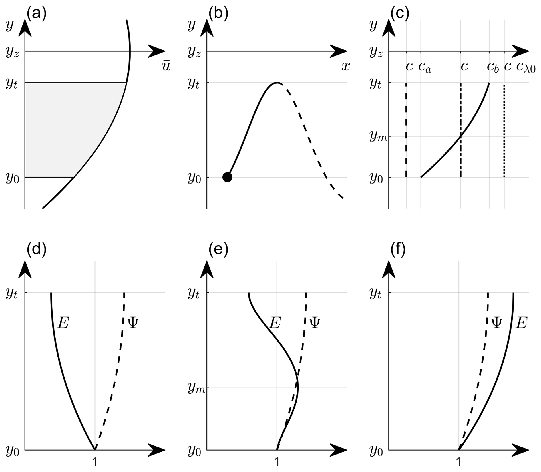
Figure 1 Schematic illustration of an ED regime that is located south of a westerly jet (a); the trajectory of a ray propagating northward from an initial location marked by the black point. The solid (dashed) black curve denotes the trajectory prior to (after) the turning point (b); the distribution of the zero point of λ (c); and the cases for c<c_a (d); $c_{\mathrm{a}}<c<c_{\mathrm{b}}$ (e); and c>c_b (f), exhibited by the dashed, dash-dotted, and dotted vertical line in (c). The notation y₀, y_t and y_z denote the initial location, the turning location, and the jet center, respectively. y_m indicates a intermediate location where c=c_λ0(y_m). E and Ψ denote wave energy and amplitude, respectively.

With above preliminaries, kl>0 and $\mathrm{d}\stackrel{\mathrm{‾}}{u}/\mathrm{d}Y>\mathrm{0}$ so that the sign of Eq. (20) is only determined by the sign of λ. According to Eq. (20), λ=0 requires its numerator equals zero, that is,

$$\begin{array}{}\text{(21)}& c^{\mathrm{2}}-{\displaystyle \frac{\mathrm{2}{k}^{\mathrm{2}}}{K^{\mathrm{2}}}}{\left(\stackrel{\mathrm{‾}}{u}-c\right)}^{\mathrm{2}}=\mathrm{0}.\end{array}$$

The solution is

$$\begin{array}{}\text{(22)}& c_{\mathit{\lambda }\mathrm{0}}\left(y\right)={\displaystyle \frac{\sqrt{\mathrm{2}}k}{K\left(y\right)+\sqrt{\mathrm{2}}k}}\stackrel{\mathrm{‾}}{u}\left(y\right).\end{array}$$

Note that c_λ0 varies along ray trajectories since $\stackrel{\mathrm{‾}}{u}$ and K varies along ray trajectories. Furthermore, when the ray moves toward the northern turning point from its initial location, $\stackrel{\mathrm{‾}}{u}$ is monotonically increasing (the ray is moving toward the jet center) while K is monotonically decreasing (caused by monotonically decreasing meridional wavenumber). Correspondingly, c_λ0 will monotonically increases from its minimum at the initial location to its maximum at the turning point, that is,

$$\begin{array}{}\text{(23)}& \begin{array}{rl}{c}_{\mathrm{a}}& \equiv {\displaystyle \frac{\sqrt{\mathrm{2}}k}{K\left(y_{\mathrm{0}}\right)+\sqrt{\mathrm{2}}k}}\stackrel{\mathrm{‾}}{u}\left(y_{\mathrm{0}}\right)=c_{\mathit{\lambda }\mathrm{0}}\left(y_{\mathrm{0}}\right)\le c_{\mathit{\lambda }\mathrm{0}}\left(y\right)\le c_{\mathit{\lambda }\mathrm{0}}\left(y_{\mathrm{t}}\right)\\ & ={\displaystyle \frac{\sqrt{\mathrm{2}}k}{K\left(y_{\mathrm{t}}\right)+\sqrt{\mathrm{2}}k}}\stackrel{\mathrm{‾}}{u}\left(y_{\mathrm{t}}\right)\equiv c_{\mathrm{b}},\end{array}\end{array}$$

where c_a and c_b denote the minimum and maximum, respectively (Fig. 1c).

If the zonal phase speed of the wave (labeled as c) is slower than c_a (illustrated by the dashed vertical line in Fig. 1c), we know c<c_λ0(y) holds on when the ray moves from its initial location to the turning point (note that c does not vary along the ray), which indicates λ<0 and hence ${\mathrm{D}}_{\mathrm{g}}E/\mathrm{D}T<\mathrm{0}$, that is, wave energy will monotonically decrease to a minimum when the ray arrives at the turning point where λ=0 due to zero meridional wavenumber (Fig. 1d). While the WKB approximation breaks down within a neighborhood to the turning point (e.g., $\left[y_{\mathrm{t}}-\mathit{\delta },y_{\mathrm{t}}\right]$ where δ≪1) , it remains asymptotically valid at the boundary of the neighborhood (at $y=y_{\mathrm{t}}-\mathit{\delta }$) . This dichotomy implies that stationary wave energy cannot physically attain the theoretical minimum value predicted at the turning point; however, this minimum serves as a critical indicator of energy thresholds prior to reflection.

If the zonal phase speed of the wave is faster than the minimum but slower than the maximum ($c_{\mathrm{a}}<c<c_{\mathrm{b}}$, illustrated by the dash–dotted vertical line in Fig. 1c), there exists an intermediate location y_m within the range (y₀,y_t) to ensure c=c_λ0(y_m) . When the ray moves from y₀ to y_m, λ>0; when the ray arrives at y_m, λ=0; and when the ray continues to move from y_m to y_t, λ<0. It means wave energy will first intensify to a maximum at y_m before decaying to a minimum at y_t (Fig. 1e). If the zonal phase speed of the wave is faster than c_b (illustrated by the dotted vertical line in Fig. 1c), we have c>c_λ0(y) , which means λ>0 and hence ${\mathrm{D}}_{\mathrm{g}}E/\mathrm{D}T>\mathrm{0}$ when the ray moves from from y₀ to y_t. Correspondingly, wave energy will monotonically increase to a maximum when the ray arrives at y_t where λ=0 due to zero meridional wavenumber (Fig. 1f).

When the ray arrives at the turning point, the local dispersion relation Eq. (4) reduces to

$$\begin{array}{}\text{(24)}& c_{y\mathrm{t}}=\stackrel{\mathrm{‾}}{u}\left(y_{\mathrm{t}}\right)-{\displaystyle \frac{{\mathit{\beta }}^{\ast }\left(y_{\mathrm{t}}\right)}{k^{\mathrm{2}}}}.\end{array}$$

Note that c_yt prescribes the possible upper limit of the zonal phase speed of a wave whose ray can propagate in an ED regime. If c>c_yt, the ray will not be reflected by any turning point along its trajectory. Since ${\mathit{\beta }}^{\ast }>\mathrm{0}$, we have $c_{y\mathrm{t}}<\stackrel{\mathrm{‾}}{u}\left(y_{\mathrm{t}}\right)$, indicating that the upper limit zonal phase speed is slower than the basic wind speed at the turning point and, naturally, slower than the maximum wind speed at the jet center.

To analyze amplitude variation, let us consider the scenario where the zonal phase speed falls within the interval (c_a,c_b) without loss of generality. Since the wave energy reaches a maximum at y_m, we have

$$\begin{array}{}\text{(25)}& \begin{array}{rl}{\left.{\displaystyle \frac{{\mathrm{D}}_{\mathrm{g}}E}{\mathrm{D}T}}\right|}_{y=y_{\mathrm{m}}}& ={\displaystyle \frac{\mathrm{1}}{\mathrm{4}}}{\left.{\displaystyle \frac{{\mathrm{D}}_{\mathrm{g}}{K}^{\mathrm{2}}}{\mathrm{D}T}}{\mathrm{\Psi }}_{\mathrm{0}}^{\mathrm{2}}\right|}_{y=y_{\mathrm{m}}}+{\displaystyle \frac{\mathrm{1}}{\mathrm{4}}}{\left.{\displaystyle \frac{{\mathrm{D}}_{\mathrm{g}}{\mathrm{\Psi }}_{\mathrm{0}}^{\mathrm{2}}}{\mathrm{D}T}}{K}^{\mathrm{2}}\right|}_{y=y_{\mathrm{m}}}\\ & =\mathrm{0},\end{array}\end{array}$$

by applying Eq. (10) – the definition of the wave energy density. The first term on the RHS is negative since the meridional wavenumber decreases monotonically. The second term must therefore be positive to enable the wave energy to reach its maximum at y_m. Consequently, the amplitude increases at y_m. When the ray arrives at y_t, the first term vanishes, and thus the second term must also vanish simultaneously, meaning that amplitude attains its maximum at the turning point. This demonstrates a monotonic increase in amplitude throughout the ray's northward trajectory (Fig. 1d, e, f).

Let's now consider a slightly complex case where the turning point lies north of the jet center, with other conditions remaining unchanged. Without loss of generality, we analyze the scenario where the zonal phase speed falls within the interval (c_a,c_b). As the ray propagates from y₀ to y_m, wave energy increases to a maximum at y_m. When the ray travels from y_m to the jet center (say, y_z) , wave energy declines from the maximum to a minimum at y_z where zero wind shear can also contribute to this minimum. As the ray proceeds from y_z to y_t, wave energy rebounds from the minimum to another maximum due to both negative wind shear and λ. Compared with the previous case, the most notable distinction is that wave energy can attain two distinct maxima as the ray propagates from the initial location to the turning point. Since analysis methodology remains consistent, we do not explicitly analyze this case.

To summarize, the evolution of wave energy and amplitude along a ray propagating in an ED regime (note that we focus here on the case where the northern turning point lies south of the jet center) depends on the wave's initial zonal phase speed. If the zonal phase speed is slower (c<c_a), wave energy undergoes monotonic decay to a minimum value at the turning point (y_t), while amplitude conversely amplifies monotonically to its maximum at this turning point. If the zonal phase speed is intermediate ($c_{\mathrm{a}}<c<c_{\mathrm{b}}$), energy exhibits nonmonotonic evolution – first intensifying to a peak at a specific point (y_m) within the region (y₀,y_m) before decaying to a minimum at y_t within the region (y_m,y_t) while amplitude monotonically amplifies to its maximum at y_t. If the zonal phase speed is faster (c>c_b) , both energy and amplitude undergo concurrent monotonic amplification, reaching their respective maxima at y_t, where maximum intensification occurs as the zonal phase speed approaches its upper bound c_yt (assuming c_yt>c_b). Note that we focus on a general theoretical analysis and thus do not prescribe an explicit profile of the westerly jet in this section. Readers who are not familiar with the above mathematical details can find specific examples for a classical westerly jet prototype in Sect. 4.

Notably, a wave with zonal phase speed in a range can develop significantly. This is strongly consistent with the bounds on zonal phase speed in the normal mode instability theory (e.g., Howard, 1961; Pedlosky, 1987). From a mathematical standpoint, rays initiating propagation from critical points – where the meridional wavenumber diverges (l²→∞) – exhibit unbounded amplification of both energy and amplitude. This divergence, however, violates the scale separation prerequisite of the WKB approximation. Physical realizability therefore imposes constraints on meridional wavenumber as well as zonal wavenumber to ensure large–scale wave dynamics.

3.2 Toward an inflection point

Let's consider a case where a ray, with an initial meridional wavenumber l₀, is just moving from an initial point y₀ to an inflection point y_i where the critical total wavenumber is K_i and corresponding meridional wavenumber is ±l_i according to Eq. (8). When the ray arrives at y_i, meridional group velocity equals zero and zonal group velocity equals zonal phase speed due to ${\mathit{\beta }}^{\ast }=\mathrm{0}$ there. It means the ray will horizontally move along y_i with a constant speed c. According to Eq. (15), wave energy at y_i can be expressed as

$$\begin{array}{}\text{(26)}& E\sim \exp \left({\mathit{\sigma }}_{i}T\right),\end{array}$$

where ${\mathit{\sigma }}_i={\left.\frac{\mathrm{2}k{l}_i}{K_i^{\mathrm{2}}}\frac{\mathrm{d}\stackrel{\mathrm{‾}}{u}}{\mathrm{d}Y}\right|}_{y=y_i}$ is a constant growth rate, the sign of which depends on the critical meridional wavenumber and meridional shear of the basic flow. Notably, a positive (negative) growth rate demonstrates exponential increase (decrease) of wave energy, and hence amplitude. The unlimited amplification of both wave energy and amplitude undoubtedly means modal instability, consistent with the critical layer problem in the classic instability theory (e.g., Pedlosky, 1987).

4 Quantitative analysis for a westerly jet prototype

To deepen our quantitative analysis of wave evolution, we utilize a prototypical westerly jet configuration previously examined by Kuo (1973), which writes as

$$\begin{array}{}\text{(27)}& \stackrel{\mathrm{‾}}{u}=u_{\mathrm{0}}{\mathrm{sech}}^{\mathrm{2}}\left({\displaystyle \frac{y}{d_{\mathrm{0}}}}\right),\end{array}$$

where u₀ is the magnitude and d₀ is a measure for width of the westerly jet (Fig. 2a). Correspondingly, the meridional gradient of absolute vorticity β^∗ becomes

$$\begin{array}{}\text{(28)}& {\mathit{\beta }}^{\ast }={\mathit{\beta }}_{\mathrm{0}}-u_{\mathrm{0}}{\mathrm{sech}}^{\mathrm{2}}\left({\displaystyle \frac{y}{d_{\mathrm{0}}}}\right){\displaystyle \frac{\mathrm{1}}{d_{\mathrm{0}}^{\mathrm{2}}}}\left[\mathrm{4}-\mathrm{6}{\mathrm{sech}}^{\mathrm{2}}\left({\displaystyle \frac{y}{d_{\mathrm{0}}}}\right)\right].\end{array}$$

It is easy to identify that β^∗ has a maximum $M={\mathit{\beta }}_{\mathrm{0}}+\frac{\mathrm{2}{u}_{\mathrm{0}}}{d_{\mathrm{0}}^{\mathrm{2}}}$ at y=0 and tends to equal to β₀ when $y\to \pm \mathrm{\infty }$ (Fig. 2b). Besides, β^∗ also has two equal minima $m={\mathit{\beta }}_{\mathrm{0}}-\frac{\mathrm{2}}{\mathrm{3}}\frac{u_{\mathrm{0}}}{d_{\mathrm{0}}^{\mathrm{2}}}$ at $y=d_{\mathrm{0}}\ln \sqrt{\mathrm{5}\pm \mathrm{2}\sqrt{\mathrm{6}}}$.

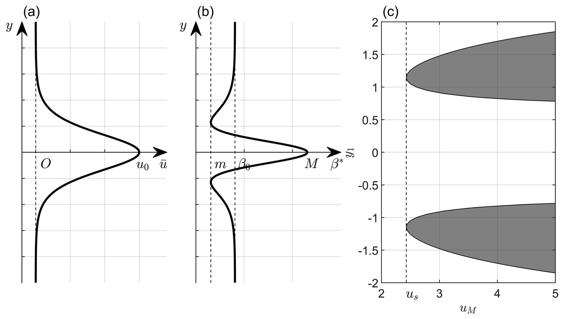
Figure 2 (a) Schematic spatial distribution of the westerly jet $\stackrel{\mathrm{‾}}{u}$ defined by Eq. (27), where u₀ denotes the jet magnitude. (b) Schematic profile of the meridional gradient of absolute vorticity β^∗ as derived from Eq. (28), where m,M represent the minimum and maximum values of β^∗, respectively, and β₀ denotes the Rossby parameter. (c) Shaded distribution of negative ${\mathit{\beta }}_{\mathrm{1}}^{\ast }$ plotted against non–dimensional meridional location y₁ and westerly jet magnitude u_M. Negative ${\mathit{\beta }}_{\mathrm{1}}^{\ast }$ occurs when $u_M>\frac{\mathrm{3}}{\mathrm{2}}{\mathit{\beta }}_{\mathrm{1}}\equiv u_s$.

By setting L=10⁶ m is the characteristic horizontal length; $U=\mathrm{10}{\mathrm{m}\mathrm{s}}^{-\mathrm{1}}$ is the characteristic value of the basic flow, and by setting

$$\begin{array}{}\text{(29)}& \begin{array}{rl}{y}_{\mathrm{1}}& ={\displaystyle \frac{y}{L}},{\stackrel{\mathrm{‾}}{u}}_{\mathrm{1}}={\displaystyle \frac{\stackrel{\mathrm{‾}}{u}}{U}},{\mathit{\omega }}_{\mathrm{1}}={\displaystyle \frac{L}{U}}\mathit{\omega },{\mathit{\beta }}_{\mathrm{1}}={\displaystyle \frac{{\mathit{\beta }}_{\mathrm{0}}{L}^{\mathrm{2}}}{U}},k_{\mathrm{1}}\\ & =kL,l_{\mathrm{1}}=lL,\end{array}\end{array}$$

where subscript “1” denote non–dimensional variables, the dispersion relation Eq. (4) is non–dimensionalized to

$$\begin{array}{}\text{(30)}& {\mathit{\omega }}_{\mathrm{1}}={\stackrel{\mathrm{‾}}{u}}_{\mathrm{1}}{k}_{\mathrm{1}}-{\displaystyle \frac{{\mathit{\beta }}_{\mathrm{1}}^{\ast }{k}_{\mathrm{1}}}{K_{\mathrm{1}}^{\mathrm{2}}}},\end{array}$$

where ${\mathit{\beta }}_{\mathrm{1}}^{\ast }={\mathit{\beta }}_{\mathrm{1}}-\frac{{\mathrm{d}}^{\mathrm{2}}{\stackrel{\mathrm{‾}}{u}}_{\mathrm{1}}}{\mathrm{d}{y}_{\mathrm{1}}^{\mathrm{2}}}$ is the non–dimensional meridional gradient of absolute vorticity. The location where ${\mathit{\beta }}_{\mathrm{1}}^{\ast }=\mathrm{0}$ (inflection points) is crucial for instability problem. According to Eq. (28), ${\mathit{\beta }}_{\mathrm{1}}^{\ast }<\mathrm{0}$ begins to emerge when the non–dimensional magnitude of the westerly jet $u_M\equiv u_{\mathrm{0}}/U>\frac{\mathrm{3}}{\mathrm{2}}{\mathit{\beta }}_{\mathrm{1}}\equiv u_{\mathrm{s}}\approx \mathrm{2.428}$ (Fig. 2c). On the other hand, according to the hurdle theorem, it is also easy to derive the sufficient condition for instability. This condition compares the hurdle with the profile of the reciprocal Rossby Mach number, which can be easily calculated from the westerly jet Eq. (27). Preliminary analysis (figures omitted) seems to suggest that ${\mathit{\beta }}_{\mathrm{1}}^{\ast }<\mathrm{0}$ may also satisfy the hurdle theorem, implying that it may also indicate a sufficient condition for instability. In the present study, we mainly focus on the energy evolution along the ray trajectory and do not explicitly discuss the application of the hurdle theorem. This aspect deserves further investigation. Note that when ${\mathit{\beta }}_{\mathrm{1}}^{\ast }>\mathrm{0}$, the westerly jet Eq. (27) is stable, as predicted by both the Rayleigh–Kuo necessary condition and the hurdle theorem. However, nonmodal instability caused by transient growth may still be possible.

The wavelength of Rossby waves can vary from synoptic scale of 10³ km order to planetary scale of 10⁴ km order. Correspondingly, the non–dimensional wavenumbers k₁ and l₁ can vary from 2π to around 0.2π. Note that we have set matched sizes for zonal and meridional wavenumbers to make sure analysis to be physically meaningful. The period for Rossby waves can vary from orders of 10¹ d to 10² d or longer (infinity for stationary waves). The corresponding non–dimensional frequency ω₁ varies from around 0.7272 to zero (for stationary waves). We do not specify explicit initial values for wave energy and amplitude because we are more concerned with the multiple by which the initial values increase. When the wave energy and amplitude exceed a certain value, thus violating the linearization approximation, the wave packet may enter the nonlinear evolution stage.

4.1 Critical locations

When ${\mathit{\beta }}_{\mathrm{1}}^{\ast }>\mathrm{0}$, the dispersion relation reduces to

$$\begin{array}{}\text{(31)}& c_{\mathrm{1}}={\stackrel{\mathrm{‾}}{u}}_{\mathrm{1}}\left(y_{\mathrm{t}}\right)-{\displaystyle \frac{{\mathit{\beta }}_{\mathrm{1}}^{\ast }\left(y_{\mathrm{t}}\right)}{k_{\mathrm{1}}^{\mathrm{2}}}}\equiv c_{y\mathrm{t}}\left(y_{\mathrm{t}}\right),\end{array}$$

at turning point y_t. Below we will consider c_yt as a function of y_t. Substituting expressions of ${\stackrel{\mathrm{‾}}{u}}_{\mathrm{1}}$ and ${\mathit{\beta }}_{\mathrm{1}}^{\ast }$, it is easy to show that if $k_{\mathrm{1}}^{\mathrm{2}}<\mathrm{8}$ (or $k_{\mathrm{1}}<\sqrt{\mathrm{8}}\equiv k_{\mathrm{c}}\approx \mathrm{2.83}$. Corresponding wavelength is around 2200 km), c_yt has three extrema, two of which, labeled as c_M, are the same maxima and the left of which, labeled as c_m, is the local minimum (see Appendix B), that is,

$$\begin{array}{}\text{(32)}& \left\{\begin{array}{l}{c}_{\mathrm{m}}\equiv c_{y\mathrm{t}}\left(\mathrm{0}\right)=u_M-\frac{{\mathit{\beta }}_{\mathrm{1}}+\mathrm{2}{u}_M}{k_{\mathrm{1}}^{\mathrm{2}}}\\ c_{\mathrm{M}}\equiv c_{y\mathrm{t}}\left(y_{\mathrm{M}}\right)=\left(k_{\mathrm{1}}^{\mathrm{2}}+\mathrm{4}\right)\left[\frac{u_M}{\mathrm{24}}-\frac{\mathrm{1}}{k_{\mathrm{1}}^{\mathrm{2}}}\left(\frac{{\mathit{\beta }}_{\mathrm{1}}}{k_{\mathrm{1}}^{\mathrm{2}}+\mathrm{4}}-\frac{u_M}{\mathrm{6}}\right)\right]\end{array}\right.,\end{array}$$

where $y_{\mathrm{M}}=\ln \left[\sqrt{\frac{\mathrm{12}}{k_{\mathrm{1}}^{\mathrm{2}}+\mathrm{4}}}\pm \sqrt{\frac{\mathrm{12}}{k_{\mathrm{1}}^{\mathrm{2}}+\mathrm{4}}-\mathrm{1}}\right]$. If $k_{\mathrm{1}}^{\mathrm{2}}>\mathrm{8}$, only c_m survives and it becomes a maximum. Besides, to make sure a ray can arrive at a turning point, c_M should be larger than zero if there are three extrema and c_m should be larger than zero if there are only one extremum. At critical point y_c, the dispersion relation reduces to

$$\begin{array}{}\text{(33)}& c_{\mathrm{1}}={\stackrel{\mathrm{‾}}{u}}_{\mathrm{1}}\left(y_{\mathrm{c}}\right)\equiv c_p\left(y_{\mathrm{c}}\right).\end{array}$$

Note that we have considered c_p as a function of y_c. Due to the same form with the basic flow, the critical point curve c_p has a maximum at y₁=0, which equals the magnitude of the westerly jet.

The meridional areas bounded by the turning points (the solid curve in Fig. 3) and the critical points (denoted by the dash-dotted curve in Fig. 3) consist of the propagative regions (Fig. 3), featured by the ED, WG, and BD regimes. When ${\mathit{\beta }}_{\mathrm{1}}^{\ast }>\mathrm{0}$, if k<k_c (Fig. 3a), rays with zonal phase speed in the range (0,c_M) propagate within the ED region. Note that in this range, there exists a subrange (c_m,c_M) where rays can propagate in both ED and WG regions. This depends on the initial location of a ray. Since we mainly focus on the propagation feature in the ED regime in this investigation, we do not explicitly analyze the cases where rays propagate in the WG regime. On the other hand, rays with zonal phase speed in range (c_M,c_p) propagate in the BD region. By contrast, if k>k_c (Fig. 3b), rays with zonal phase speed in (0,c_m) propagate within the ED region, while those in (c_m,c_p) fall into the BD region.

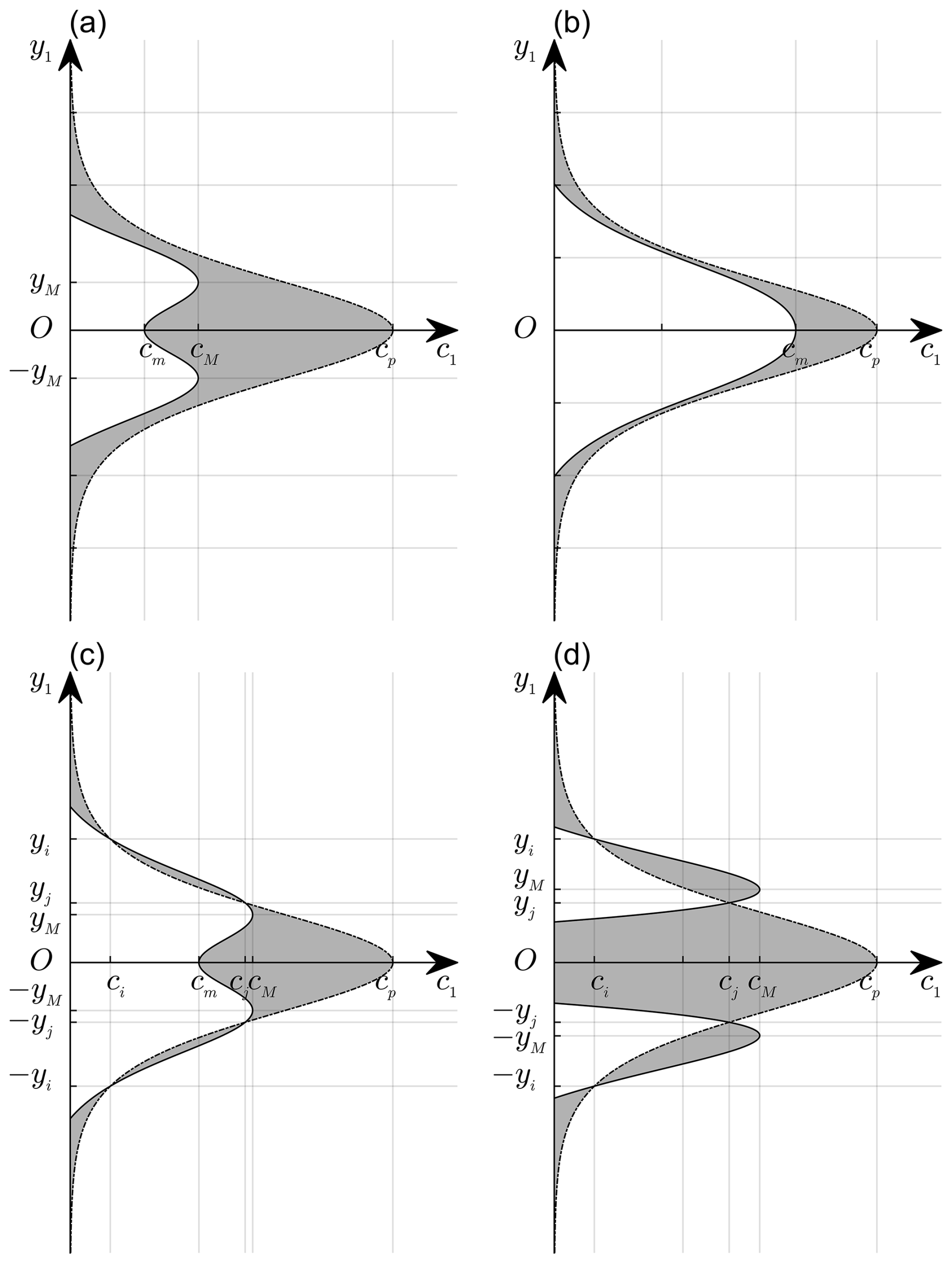
Figure 3 Schematic illustration of shaded propagation regions bounded by turning points (solid curve) and critical points (dash–dotted curves) under varying ${\mathit{\beta }}_{\mathrm{1}}^{\ast }$ and zonal wavenumber conditions: (a) ${\mathit{\beta }}_{\mathrm{1}}^{\ast }>\mathrm{0}$ and $k_{\mathrm{1}}<\sqrt{\mathrm{8}}$; (b) ${\mathit{\beta }}_{\mathrm{1}}^{\ast }>\mathrm{0}$ and $k_{\mathrm{1}}>\sqrt{\mathrm{8}}$; (c) ${\mathit{\beta }}_{\mathrm{1}}^{\ast }<\mathrm{0}$, $k_{\mathrm{1}}<\sqrt{\mathrm{8}}$, and $-y_j<-y_{\mathrm{M}}<\mathrm{0}$; (d) ${\mathit{\beta }}_{\mathrm{1}}^{\ast }<\mathrm{0}$, $k_{\mathrm{1}}<\sqrt{\mathrm{8}}$, and $-y_{\mathrm{M}}<-y_j<\mathrm{0}$. Intersection points of inflection and critical points occur at y_i and y_j ($y_i>y_j>\mathrm{0}$) . Labels y_M and c_M denote the meridional location of turning point curve maximum and its corresponding zonal phase speed under condition $k_{\mathrm{1}}<\sqrt{\mathrm{8}}$. c_m represents maximum zonal phase speed associated with turning point curve under condition $k_{\mathrm{1}}>\sqrt{\mathrm{8}}$. c_i and c_j correspond to zonal phase speeds at intersection points y_i and y_j, respectively. c_p denotes the zonal phase speed at the critical point curve maximum. The specific values are k₁=2, u_M=1.5 for (a); k₁=3.5, u_M=1.5 for (b); k₁=2, u_M=4 for (c); and k₁=1, u_M=4 for (d).

When ${\mathit{\beta }}_{\mathrm{1}}^{\ast }<\mathrm{0}$, intersection points between turning and critical points emerge at ${\mathit{\beta }}_{\mathrm{1}}^{\ast }=\mathrm{0}$. We focus on our analysis to regions (y₁<0) with positive wind shear. Let the two intersection points be located at −y_i and −y_j ($-y_i<-y_j<\mathrm{0}$), with corresponding zonal phase speeds labeled c_i and c_j (c_i<c_j) , as illustrated in Fig. 3c and d. When $-y_j<-y_{\mathrm{M}}$, the propagation scenario (Fig. 3c) mirrors the ${\mathit{\beta }}_{\mathrm{1}}^{\ast }>\mathrm{0}$ case in Fig. 3a, that is, rays with zonal phase speed in (0,c_M) propagates within the ED region (note that we have neglected the WG region). Conversely, when $-y_j>-y_{\mathrm{M}}$, the zonal phase speed range defining the ED regions shrinks to (0,c_j) while the remaining (c_j,c_M) range transfers to a small WG region (Fig. 3d).

4.2 Wave evolution in the ED region

Building on the preceding analysis, the zonal phase speed range defining the ED region is determined by critical thresholds c_m, c_M, or c_j, which we collectively denote as c_max for simplicity (where c_max corresponds to c_m, c_M, or c_j depending on the basic flow configuration). Consistent with prior theoretical analysis in Sect. 3, this interval $\left(\mathrm{0},c_{max}\right)$ can be partitioned into three contiguous subranges – (0,c_a) , (c_a,c_b), and $\left(c_{\mathrm{b}},c_{max}\right)$ – as illustrated in Fig. 4. Within these subranges, wave energy evolution follows distinct patterns: in (0,c_a), energy decays monotonically to a minimum at the turning point; in (c_a,c_b), it first amplifies to a maximum before decaying to a local minimum at the turning point; and in $\left(c_{\mathrm{b}},c_{max}\right)$, it amplifies monotonically, peaking at the turning point. Amplitude, by contrast, demonstrates uniform monotonic growth across the entire $\left(\mathrm{0},c_{max}\right)$ range, reaching its maximum precisely at the turning point. The amplification of wave energy toward the turning points aligns with transient growth mechanisms in barotropic Rossby waves within uniformly sheared basic flows (e.g., Tung, 1983; Yamagata, 1976). The present study extends these findings to more generalized basic flows, where analytical solutions for initial–value problems remain intractable, thereby enhancing the applicability of transient growth theory to non–uniform shear environments.

Figure 4 further reveals that both wave energy and amplitude at the turning point are monotonically increasing functions of zonal phase speed, which is consistent with the theoretical prediction in Sect. 3. For a wave with fixed zonal wavenumber, this implies that maximum transient growth of both energy and amplitude occurs when the zonal phase speed reaches c_max. In other words, c_max corresponds to the zonal phase speed at which waves with fixed wavenumbers exhibit the most significant development (Fig. 4a) or even transition to potential instability (Fig. 4b). To focus our analysis, we examine the evolution of wave energy and amplitude for rays with zonal phase speed equal to c_max, which is readily identifiable (Fig. 5) owing to the analytical westerly jet model. As illustrated in Fig. 5, the $c_{max}\left(k_{\mathrm{1}},u_M\right)=\mathrm{0}$ curve exhibits monotonic decay with increasing zonal wavenumber. Below this curve, the dashed contour indicates that rays do not encounter any turning point along their trajectories. Above the curve, the farther a point lies from the curve, the more rapidly the energy amplification rate becomes. Additionally, a second critical curve (c_M=c_j) emerges (red solid curve in Fig. 5), above which the amplification rate become independent of zonal wavenumber and instead increases monotonically with the intensity of the westerly jet. This configuration corresponds to scenarios where c_max assumes the value of c_j rather than c_m or c_M as depicted in Fig. 3d.

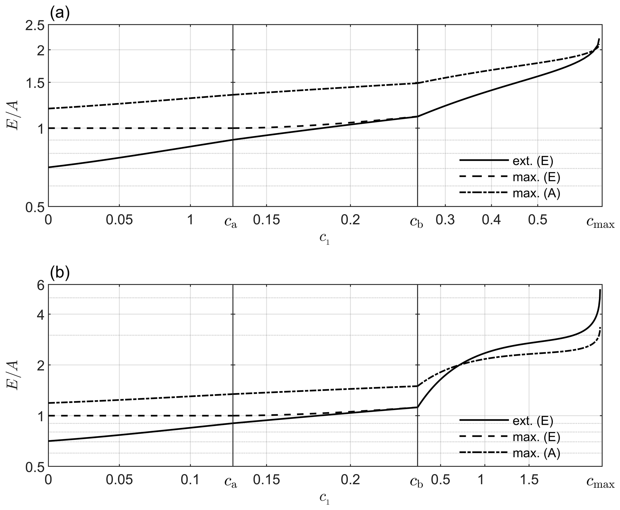
Figure 4 Variation of wave energy at turning points (solid curve), maximum wave energy (dashed curve), and maximum amplitude (dash–dotted curve) with zonal phase speed c₁. (a) For a case where u_M=1.5; (b) for a case where u_M=4.0. The wavelength is fixed as 3000 km (corresponding to a zonal wavenumber k≃2.1). Symbols c_a≃0.13, c_b≃0.24 denote divisions of zonal phase range $\left(\mathrm{0},c_{max}\right)$ where $c_{max}\simeq \mathrm{0.63}$ specific to (a) and $c_{max}\simeq \mathrm{2.3}$ specific to (b). In (0,c_a) , energy decays monotonically to minima at turning points; in (c_a,c_b) it first amplifies to maxima before decaying to local minima at turning points; and in $\left(c_{\mathrm{b}},c_{max}\right)$ , it amplifies monotonically, peaking at turning points. By contrast, amplitude demonstrates uniform monotonic growth across in $\left(\mathrm{0},c_{max}\right)$ , reaching its maxima at turning points. Initial values of both wave energy and amplitude are normalized to unity.

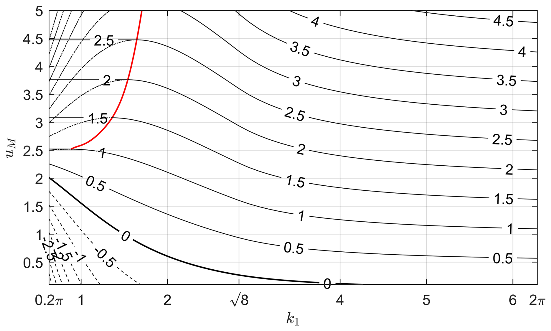
Figure 5 Contour plot of c_max (solid contour lines) as a function of zonal wavenumber k₁ and westerly jet magnitude u_M. The dashed contour denotes regions where the ED propagation regime does not exist due to $c_{max}<\mathrm{0}$. The red curve marks the critical threshold c_M=c_j. Above this curve, the dash–dotted contours represent c_M is superseded by c_j as the effective upper bound of the ED region due to the propagation dynamics depicted in Fig. 3d.

Figure 6 further illustrated the maxima of wave energy (Fig. 6a) and amplitude (Fig. 6b) at turning points for ray with zonal phase speed c_max. Given the amplitude's evolutionary pattern closely mirrors wave energy but with reduced magnitude, we focus our analysis on amplitude dynamics. For weak jet intensities – particularly when u_M<2.428 (precluding normal mode instability) – transient growth upon reaching the turning point remains moderate. Consequently, Rossby waves exhibit moderate growth without transitioning to instability. By contrast, for jet intensities exceeding a critical threshold (e.g., u_M>3.0) , an optimal zonal wavenumber (or corresponding wavelength) emerges, coinciding with the strongest transient amplitude growth. For instance, when u_M=4.0, a ray with k₁=1 (wavelength is around 6000 km) amplifies to around 7.4 times its initial amplitude upon reaching the turning point (wave energy has a larger amplification). Although amplitude decays post–reflection from the turning point, the transient amplification is sufficient large to potentially trigger nonmodal instability. As jet intensity increases, the optimal zonal wavenumber shifts upward. When u_M=5.0, this optimal wavenumber corresponds to k₁≃1.1 (wavelength is around 5500 km). Notably, the optimal zonal wavenumber lies above the c_j=c_M defined boundary from Fig. 5 (reproduced in Fig. 6 for comparison). This indicates that the optimal zonal wavenumber resides within the ray propagation regime characterized in Fig. 3d.

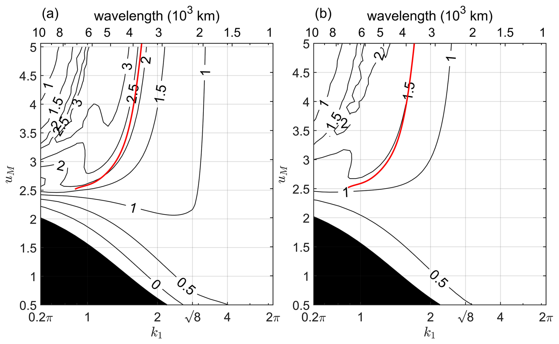
Figure 6 Logarithm of wave energy (a) and amplitude (b) at turning points for rays with zonal phase speed c_max (as defined in Fig. 5). The regions where the ED regime is absent is masked. Initial wave energy and amplitude are normalized to unity.

4.3 The critical layer problem

When a ray traverses a critical layer – a phenomenon extensively studied in geophysical fluid dynamics (e.g., Pedlosky, 1987) – we also focus on the region south of the jet center where meridional shear is positive. Consider a ray (solid curve in Fig. 7a) with zonal phase seed c_max (equivalent to c_j) propagating southward ($c_{g,y}<\mathrm{0}$ hence initial meridional wavenumber l₀<0) from an initial location −y₀ toward the inflection point −y_i (also the critical point). Along this trajectory, the negative meridional wavenumber (solid curve in Fig. 7b) increases monotonically to the negative critical value −l_i, then stabilizes as dictated by Eq. (8). This negative wavenumber corresponds to a negative growth rate, driving decay of both wave energy and amplitude (solid curve in Fig. 7c). Similarly, a northward–propagating ray (dashed curve in Fig. 7a) originating from −y₀ must also exhibit a negative meridional wavenumber (dashed curve in Fig. 7b) to satisfy the positive meridional group velocity constraint. Upon reaching the inflection point −y_i, this negative critical meridional wavenumber −l_i similarly induces a negative growth rate, resulting in declining energy and amplitude (dashed curve in Fig. 7c). In contrast, rays propagating southward from an initial location −y₀ ($-y_{\mathrm{0}}<-y_i$) encounter a southern turning point, where they undergo significant transient amplification. This pre–turning–point growth – sufficient to trigger nonmodal instability – renders reflection dynamics at the turning point less critical to the overall instability process.

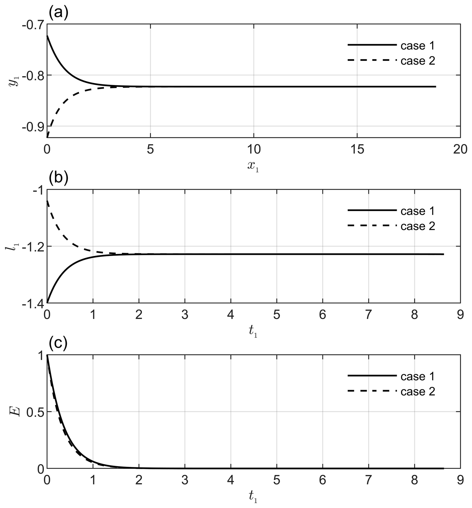
Figure 7 (a) Ray trajectories; (b) evolution of meridional wavenumber along rays; (c) wave energy evolution along rays. The solid (dashed) curve corresponds to a ray propagating southward (northward) the inflection point $y_j=-\mathrm{0.8227}$ from an initial location $y_{\mathrm{0}}=y_i\pm \mathrm{0.1}$. Zonal wavenumber k₁=1; zonal phase speed $c_{max}=\mathrm{2.1692}$; and westerly jet magnitude u_M=4.

Consider a ray originating exactly at the inflection point ($-y_{\mathrm{0}}=-y_j$). Owing to $c_{g,y}=\mathrm{0}$, the ray propagates zonally with the zonal group velocity that equals the zonal phase speed c_max (Fig. 8a). Although the initial meridional wavenumber l₀ at the inflection point is unconstrained, its evolution remains governed by the second equation in Eq. (7), that is, $\frac{{\mathrm{D}}_{\mathrm{g}}l}{\mathrm{D}T}\equiv -\frac{\partial \mathrm{\Omega }}{\partial Y}$. Within the prototype westerly jet, |l₀|<l_i drives $\frac{{\mathrm{D}}_{\mathrm{g}}l}{\mathrm{D}T}>\mathrm{0}$, while |l₀|>l_i induces $\frac{{\mathrm{D}}_{\mathrm{g}}l}{\mathrm{D}T}<\mathrm{0}$. Consequently, as Fig. 8b illustrated, if |l₀|<l_i (dashed curve) or l₀>l_i (solid curve), the meridional wavenumber approaches l_i; if $l_{\mathrm{0}}<-l_i$ (dash–dotted curve), it monotonically decrease toward negative infinity. Correspondingly, wave energy exhibits exponential growth when meridional wavenumber approaches l_i (solid and dashed curves in Fig. 8c) but decays exponentially when the meridional wavenumber tends toward negative infinity (dash–dotted curve in Fig. 8c).

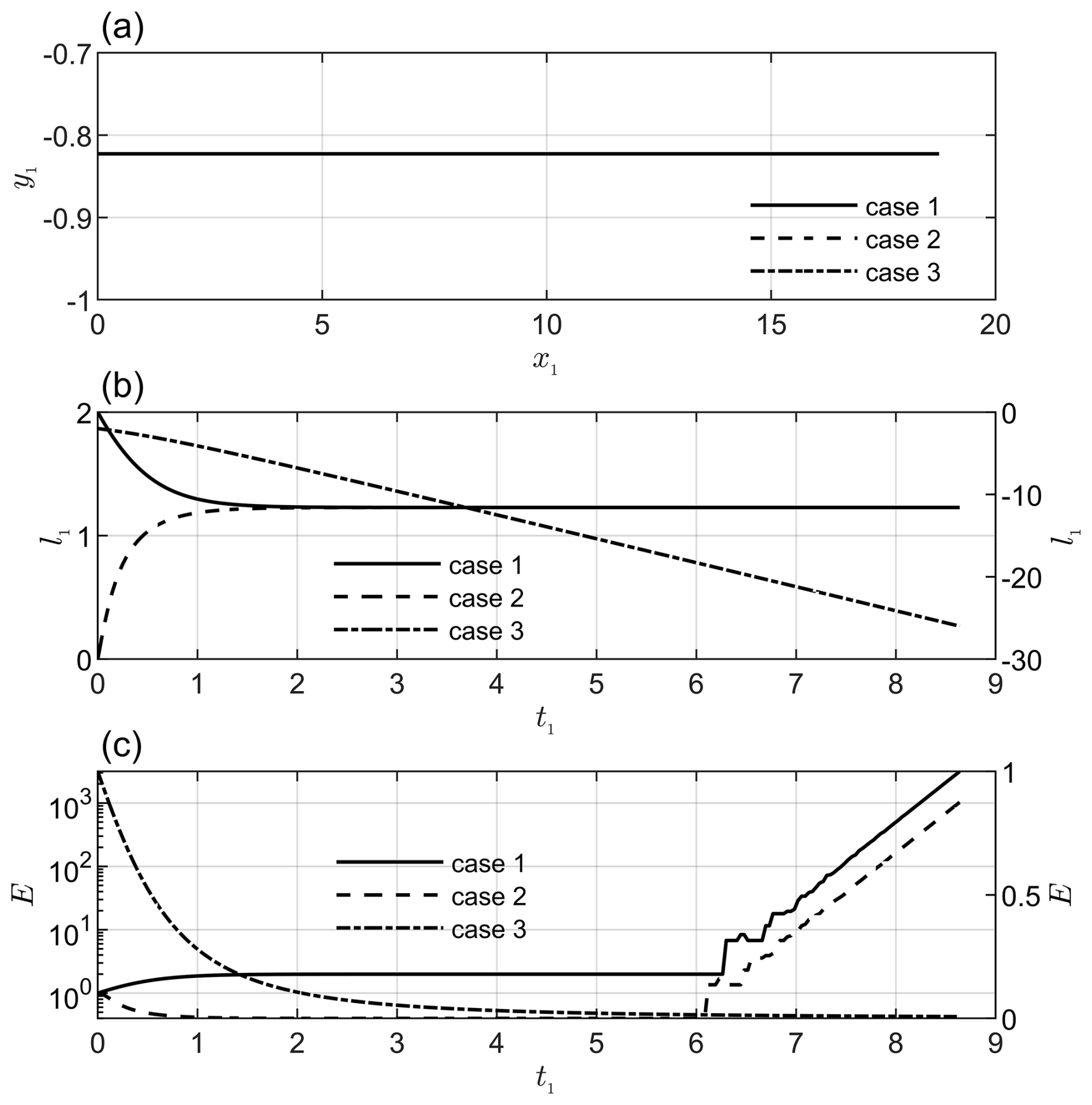
Figure 8 (a) Ray trajectories; (b) evolutionary of meridional wavenumber along ray trajectories; (c) wave energy evolution along ray trajectories. Initial meridional wavenumbers are assigned values of 2, 0, and −2, denoted by solid, dashed, and dash–dotted curves (labeled as Case 1, Case 2, and Case 3, respectively). Right–hand y-axes in panels (b) and (c) correspond to Case 3 for scale clarity. Zonal wavenumber k₁=1; zonal phase speed $c_{max}=\mathrm{2.1692}$; initial meridional location $y_{\mathrm{0}}=-y_j=\mathrm{0.8227}$; and westerly jet magnitude u_M=4, respectively.

5 Conclusions and discussion

The physical understanding behind Rossby wave instability has been investigated for several decades. Recent advances in the context of the reciprocal Rossby Mach number (Deguchi et al., 2024) yield a sufficient condition guaranteeing instability in a class of basic flows, shedding the latest insights into the classical problem. However, a general comprehension of Rossby wave instability in generalized basic flow setups, which may help to interpret synoptic scale variability such as extreme weather events, is still an open question. This study re–examines classical barotropic instability through the lens of Rossby wave ray–tracing theory and wave action conservation. This focus on barotropic instability is not motivated by overemphasizing its role; rather, it is chosen because it offers a clean theoretical framework for investigating instability in a controlled dynamical setting. Analytical solutions reveal that wave energy evolution along ray trajectories exhibits two key dependencies: directly proportional to intrinsic frequency and inversely proportional to group velocity magnitude. Notably, wave energy attains extrema at turning points where group velocity magnitude reaches extremal values. A critical constraint emerges for rays to encounter a turning point during propagation, that is, zonal phase speed must remain below an upper limit determined by dispersion relation at the turning point.

Three distinct energy evolution patterns are theoretically identified: (1) energy minima at turning points, (2) pre–turning–point maxima followed by decline to local minima, and (3) energy maxima at turning points under continuously accelerating zonal phase speed. On the contrast, wave amplitude maximizes at turning points. These findings suggest that there exists a zonal phase speed range where simultaneous energy and amplitude growth means significant development of Rossby waves. Particularly, waves propagate with zonal phase speed equal to the upper limit is the most favorably developing. This provides dynamical support for Howard's (1961) semicircle theorem governing unstable waves.

The inherent symmetry of ray trajectories about a turning point creates complementary energy–amplitude evolution: growth towards a turning point will be counterbalanced by subsequent decay. This mechanism explains the transient growth phenomenon first identified by Orr (1907) and later recognized as crucial for initiating nonmodal instability (e.g., Boyd, 1983; Farrell, 1984; Trefethen et al., 1993). At inflection points where meridional gradient of absolute vorticity vanishes, rays exhibit horizontal propagation with zonal phase speed that equals to zonal group velocity. Here, the wave energy growth rate is determined by the product of the critical meridional wavenumber and wind shear. A positive growth rate directly triggers the exponential amplification characteristic of modal instability.

Quantitative calculation of a prototype westerly jet reveal critical insights into transient Rossby wave dynamics. When the Rayleigh–Kuo instability criterion remains unsatisfied, transient growth for Rossby waves with synoptic wavelengths proves to be moderate–a finding that aligns with their typical developmental (rather than destabilizing) behavior in such configuration. When the Rayleigh–Kuo criterion becomes satisfied, transient growth intensifies substantially to induce potential nonmodal instability when ray trajectories approach turning points, particularly when inflection points are accessible for rays. At inflection points, where absolute vorticity gradients vanish, the emergence of constant positive growth rate will drive exponential energy accumulation, a hallmark of modal instability. Crucially, our analysis demonstrates that inflection points, if accessible for rays, serve as a primary standard for instability manifestation. This mechanism operates through sustained exponential growth characteristic of modal instability when rays approach inflection points with positive growth rate on the one hand, and via enhanced transient growth to trigger possible nonmodal instability when rays propagating toward turning points on the other hand. Besides, the zonal phase speed at an accessible inflection point for rays coincides with the zonal wind shift, which is precisely the zonal phase speed of an unstable wave in the hurdle theorem.

The proposed analysis approach in this investigation has potential applications in the future. It not only provides a systematic assessment of Rossby wave evolution and instability for a range of prescribed basic flow profiles within a barotropic framework. More importantly, the methodology permits a natural extension to baroclinic systems. Such extensions would allow the current barotropic insights to be bridged with more realistic atmospheric basic flows, where vertical shear and stratification often dominate Rossby wave evolution. Correspondingly, by specifying realistic atmospheric basic flows, practitioners can systematically identify turning points governing wave reflection, critical points regulating phase speed matching, and inflection points controlling modal instability onset. This diagnostic capability enables two practical applications: (1) optimization of disturbance parameters through precise determination of wavelength/wavenumber combinations that maximize transient amplification potential, and (2) quantitative tracking of energy–amplitude co–evolution via closed–form analytical expressions. This theoretical foundation ultimately provides a pathway towards a unified understanding of instability (whether modal or nonmodal) in both barotropic and baroclinic flows, and thereby offers a framework that, after appropriate extension, can be applied to real-world atmospheric contexts. In addition, the current version lacks topography, which may be insufficient when investigating the influence of large–scale topography on wave evolution along rays in the real–world atmosphere. Moreover, in giant gas planets such as Jupiter and Saturn, where a deep–layer jet, serving as a dynamical topography, also plays a significant role in modulating the weather layer above it. All these deserve further investigation.

Appendix A: Derivation of the Wave Energy Equation Along Ray Trajectories

Applying the definition of the wave action density, Eq. (11) can be written as

$$\begin{array}{}\text{(A1)}& {\displaystyle \frac{\mathrm{1}}{E}}{\displaystyle \frac{{\mathrm{D}}_{\mathrm{g}}E}{\mathrm{D}T}}-{\displaystyle \frac{\mathrm{1}}{{\mathit{\omega }}^{\prime }}}{\displaystyle \frac{{\mathrm{D}}_{\mathrm{g}}{\mathit{\omega }}^{\prime }}{\mathrm{D}T}}+\mathrm{\nabla }\cdot {\mathit{c}}_{\mathrm{g}}=\mathrm{0}.\end{array}$$

Since ${\mathit{\omega }}^{\prime }=\mathit{\omega }-\stackrel{\mathrm{‾}}{u}k=-{\mathit{\beta }}^{\ast }k/K^{\mathrm{2}}$, the second term in (A1) can be expanded as

$$\begin{array}{}\text{(A2)}& -{\displaystyle \frac{\mathrm{1}}{{\mathit{\omega }}^{\prime }}}{\displaystyle \frac{{\mathrm{D}}_{\mathrm{g}}{\mathit{\omega }}^{\prime }}{\mathrm{D}T}}={\displaystyle \frac{K^{\mathrm{2}}}{{\mathit{\beta }}^{\ast }k}}\left({\displaystyle \frac{{\mathrm{D}}_{\mathrm{g}}\mathit{\omega }}{\mathrm{D}T}}-{\displaystyle \frac{{\mathrm{D}}_{\mathrm{g}}\stackrel{\mathrm{‾}}{u}k}{\mathrm{D}T}}\right)=-{\displaystyle \frac{K^{\mathrm{2}}}{{\mathit{\beta }}^{\ast }}}{\displaystyle \frac{{\mathrm{D}}_{\mathrm{g}}\stackrel{\mathrm{‾}}{u}}{\mathrm{D}T}}.\end{array}$$

Note that we have applied Eq. (7) which demonstrates that the material derivatives along rays for frequency and zonal wavenumber are zero since the basic flow $\stackrel{\mathrm{‾}}{u}\left(Y\right)$ is independent of T and X. Correspondingly, the material derivative for $\stackrel{\mathrm{‾}}{u}$ can be expanded as

$$\begin{array}{}\text{(A3)}& {\displaystyle \frac{{\mathrm{D}}_{\mathrm{g}}\stackrel{\mathrm{‾}}{u}}{\mathrm{D}T}}={\displaystyle \frac{\partial \stackrel{\mathrm{‾}}{u}}{\partial T}}+c_{g,x}{\displaystyle \frac{\partial \stackrel{\mathrm{‾}}{u}}{\partial X}}+c_{g,y}{\displaystyle \frac{\partial \stackrel{\mathrm{‾}}{u}}{\partial Y}}=c_{g,y}{\displaystyle \frac{\mathrm{d}\stackrel{\mathrm{‾}}{u}}{\mathrm{d}Y}}={\displaystyle \frac{\mathrm{2}{\mathit{\beta }}^{\ast }kl}{K^{\mathrm{4}}}}{\displaystyle \frac{\mathrm{d}\stackrel{\mathrm{‾}}{u}}{\mathrm{d}Y}}.\end{array}$$

Note that we have replaced $\frac{\partial \stackrel{\mathrm{‾}}{u}}{\partial Y}$ with $\frac{\mathrm{d}\stackrel{\mathrm{‾}}{u}}{\mathrm{d}Y}$. Substituting Eqs. (A3) and (A2) into Eq. (A1), we can derive

$$\begin{array}{}\text{(A4)}& {\displaystyle \frac{\mathrm{1}}{E}}{\displaystyle \frac{{\mathrm{D}}_{\mathrm{g}}E}{\mathrm{D}T}}-{\displaystyle \frac{\mathrm{2}kl}{K^{\mathrm{2}}}}{\displaystyle \frac{\mathrm{d}\stackrel{\mathrm{‾}}{u}}{\mathrm{d}Y}}+\mathrm{\nabla }\cdot {\mathit{c}}_{\mathrm{g}}=\mathrm{0}.\end{array}$$

Substituting Eq. (12) into Eq. (A4), we can immediately derive the wave energy equation along ray trajectories, that is,

$$\begin{array}{}\text{(A5)}& {\displaystyle \frac{\mathrm{1}}{E}}{\displaystyle \frac{{\mathrm{D}}_{\mathrm{g}}E}{\mathrm{D}T}}={\displaystyle \frac{\mathrm{2}kl}{K^{\mathrm{2}}}}{\displaystyle \frac{\mathrm{d}\stackrel{\mathrm{‾}}{u}}{\mathrm{d}Y}}-{\displaystyle \frac{{\mathrm{D}}_{\mathrm{g}}\ln \left|{\mathit{c}}_{\mathrm{g}}\right|}{\mathrm{D}T}}\equiv \mathit{\xi }\left(T\right).\end{array}$$

Appendix B: Extremum Analysis of Zonal Phase Speed at Turning Points

The non-dimensional basic flow and meridional gradient of the absolute vorticity for basic flow can be written as

$$\begin{array}{}\text{(B1)}& \left\{\begin{array}{l}{\stackrel{\mathrm{‾}}{u}}_{\mathrm{1}}=u_M{\mathrm{sech}}^{\mathrm{2}}\left(y_{\mathrm{1}}\right)\\ {\mathit{\beta }}_{\mathrm{1}}^{\ast }={\mathit{\beta }}_{\mathrm{1}}-\frac{{\mathrm{d}}^{\mathrm{2}}{\stackrel{\mathrm{‾}}{u}}_{\mathrm{1}}}{\mathrm{d}{y}_{\mathrm{1}}^{\mathrm{2}}}\end{array}\right..\end{array}$$

Substituting Eq. (B1) into Eq. (31), we have

$$\begin{array}{}\text{(B2)}& \begin{array}{rl}{c}_{y\mathrm{t}}& \equiv c_{\mathrm{1}}\left(y_{\mathrm{t}}\right)=u_M{\mathrm{sech}}^{\mathrm{2}}\left(y_{\mathrm{t}}\right)-{\displaystyle \frac{\mathrm{1}}{k_{\mathrm{1}}^{\mathrm{2}}}}\left[{\mathit{\beta }}_{\mathrm{1}}-\mathrm{4}{u}_M{\mathrm{sech}}^{\mathrm{2}}\left(y_{\mathrm{t}}\right)\right.\\ & \left.+\mathrm{6}{u}_M{\mathrm{sech}}^{\mathrm{4}}\left(y_{\mathrm{t}}\right)\right],\end{array}\end{array}$$

where y_t denotes the non-dimensional location of the turning point. Now we consider c_yt as a function of y_t, with its derivative being

$$\begin{array}{}\text{(B3)}& \begin{array}{rl}{\displaystyle \frac{\mathrm{d}{c}_{y\mathrm{t}}}{\mathrm{d}{y}_{\mathrm{t}}}}& =-{\displaystyle \frac{\mathrm{2}{u}_M}{k_{\mathrm{1}}^{\mathrm{2}}}}\left(k_{\mathrm{1}}^{\mathrm{2}}+\mathrm{4}\right)\sinh \left(y_{\mathrm{t}}\right)\left[{\cosh }^{\mathrm{2}}\left(y_{\mathrm{t}}\right)-{\displaystyle \frac{\mathrm{12}}{k_{\mathrm{1}}^{\mathrm{2}}+\mathrm{4}}}\right]\\ & {\mathrm{sech}}^{\mathrm{5}}\left(y_{\mathrm{t}}\right).\end{array}\end{array}$$

To identify the extreme values of c_yt, we solve the zero point of Eq. (B3), which satisfies

$$\begin{array}{}\text{(B4)}& \sinh \left(y_{\mathrm{t}}\right)\left[{\cosh }^{\mathrm{2}}\left(y_{\mathrm{t}}\right)-{\displaystyle \frac{\mathrm{12}}{k_{\mathrm{1}}^{\mathrm{2}}+\mathrm{4}}}\right]=\mathrm{0}.\end{array}$$

It is easy to identify that y_t=0 is a zero point. The other zero points satisfy

$$\begin{array}{}\text{(B5)}& {\cosh }^{\mathrm{2}}\left(y_{\mathrm{t}}\right)={\displaystyle \frac{\mathrm{12}}{k_{\mathrm{1}}^{\mathrm{2}}+\mathrm{4}}},\end{array}$$

Since |cosh (y)|≥1, to make sure Eq. (B5) has real roots, we have $k_{\mathrm{1}}^{\mathrm{2}}\le \mathrm{8}$. Setting $z=e^{y_{\mathrm{t}}}$ and substituting it into Eq. (B5), we can obtain

$$\begin{array}{}\text{(B6)}& z+{\displaystyle \frac{\mathrm{1}}{z}}=\mathrm{2}\sqrt{{\displaystyle \frac{\mathrm{12}}{k_{\mathrm{1}}^{\mathrm{2}}+\mathrm{4}}}},\end{array}$$

whose solution is

$$\begin{array}{}\text{(B7)}& z=\sqrt{{\displaystyle \frac{\mathrm{12}}{k_{\mathrm{1}}^{\mathrm{2}}+\mathrm{4}}}}\pm \sqrt{{\displaystyle \frac{\mathrm{12}}{k_{\mathrm{1}}^{\mathrm{2}}+\mathrm{4}}}-\mathrm{1}}.\end{array}$$

Then it is easy to get the solution for Eq. (B5), that is

$$\begin{array}{}\text{(B8)}& y_{\mathrm{t}}=\ln \left[\sqrt{{\displaystyle \frac{\mathrm{12}}{k_{\mathrm{1}}^{\mathrm{2}}+\mathrm{4}}}}\pm \sqrt{{\displaystyle \frac{\mathrm{12}}{k_{\mathrm{1}}^{\mathrm{2}}+\mathrm{4}}}-\mathrm{1}}\right]\equiv y_{\mathrm{M}}\end{array}$$

To identify the relative size of these extreme values, we further derive the second derivative

$$\begin{array}{}\text{(B9)}& \begin{array}{rl}{\displaystyle \frac{{\mathrm{d}}^{\mathrm{2}}{c}_{y\mathrm{t}}}{\mathrm{d}{y}_{\mathrm{t}}^{\mathrm{2}}}}& ={\displaystyle \frac{\mathrm{2}{u}_M}{k_{\mathrm{1}}^{\mathrm{2}}}}\left[\mathrm{2}\left(k_{\mathrm{1}}^{\mathrm{2}}+\mathrm{4}\right){\sinh }^{\mathrm{4}}\left(y_{\mathrm{t}}\right)-\mathrm{44}{\sinh }^{\mathrm{2}}\left(y_{\mathrm{t}}\right)\right.\\ & \left.+k_{\mathrm{1}}^{\mathrm{2}}{\sinh }^{\mathrm{2}}\left(y_{\mathrm{t}}\right)+\mathrm{8}-k_{\mathrm{1}}^{\mathrm{2}}\right]{\mathrm{sech}}^{\mathrm{6}}\left(y_{\mathrm{t}}\right).\end{array}\end{array}$$

According to Eq. (B5), we have

$$\begin{array}{}\text{(B10)}& {\sinh }^{\mathrm{2}}\left(y_{\mathrm{t}}\right)={\displaystyle \frac{\mathrm{8}-k_{\mathrm{1}}^{\mathrm{2}}}{k_{\mathrm{1}}^{\mathrm{2}}+\mathrm{4}}}.\end{array}$$

Substituting Eq. (B10) into Eq. (B9), we have

$$\begin{array}{}\text{(B11)}& {\left.{\displaystyle \frac{{\mathrm{d}}^{\mathrm{2}}{c}_{y\mathrm{t}}}{\mathrm{d}{y}_{\mathrm{t}}^{\mathrm{2}}}}\right|}_{y_{\mathrm{t}}=y_{\mathrm{M}}}=-\mathrm{48}{\displaystyle \frac{u_M}{k_{\mathrm{1}}^{\mathrm{2}}}}{\displaystyle \frac{\mathrm{8}-k_{\mathrm{1}}^{\mathrm{2}}}{k_{\mathrm{1}}^{\mathrm{2}}+\mathrm{4}}}{\mathrm{sech}}^{\mathrm{6}}\left(y_{\mathrm{M}}\right)<\mathrm{0}.\end{array}$$

Therefore, we can identify c_yt reaches the maxima at y_M. On the other hand,

$$\begin{array}{}\text{(B12)}& {\left.{\displaystyle \frac{{\mathrm{d}}^{\mathrm{2}}{c}_{y\mathrm{t}}}{\mathrm{d}{y}_{\mathrm{t}}^{\mathrm{2}}}}\right|}_{y_{\mathrm{t}}=\mathrm{0}}=\mathrm{8}-k_{\mathrm{1}}^{\mathrm{2}}>\mathrm{0}.\end{array}$$

Therefore, we can identify c_yt reaches a local minimum at y_1t=0. When $k_{\mathrm{1}}^{\mathrm{2}}>\mathrm{8}$ this local minimum becomes the only maximum. Substituting y_t=0 and y_t=y_M into Eq. (B2), we can get the expressions of the local minimum and maxima, which writes as

$$\begin{array}{}\text{(B13)}& \left\{\begin{array}{l}{c}_{\mathrm{m}}\equiv c_{y\mathrm{t}}\left(\mathrm{0}\right)=u_M-\frac{{\mathit{\beta }}_{\mathrm{1}}+\mathrm{2}{u}_M}{k_{\mathrm{1}}^{\mathrm{2}}}\\ c_{\mathrm{M}}\equiv c_{y\mathrm{t}}\left(y_{\mathrm{M}}\right)=\left(k_{\mathrm{1}}^{\mathrm{2}}+\mathrm{4}\right)\left[\frac{u_M}{\mathrm{24}}-\frac{\mathrm{1}}{k_{\mathrm{1}}^{\mathrm{2}}}\left(\frac{{\mathit{\beta }}_{\mathrm{1}}}{k_{\mathrm{1}}^{\mathrm{2}}+\mathrm{4}}-\frac{u_M}{\mathrm{6}}\right)\right]\end{array}\right..\end{array}$$