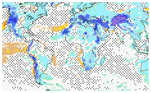
Advective, adiabatic and diabatic contributions to heat extremes simulated with the Community Earth System Model version 2

Do heat extremes in climate model simulations form for the right physical reasons? Addressing this question is essential to further our confidence in heat extreme projections, to pinpoint regionally varying model biases, and to enable model improvements regarding heat extremes. Here, we perform a detailed process-based evaluation of CMIP6-type simulations with the Community Earth System Model version 2 (CESM2) regarding heat extremes and employ a previously established Lagrangian approach to quantify advective, adiabatic, and diabatic contributions to near-surface temperature anomalies (T^′) during heat extremes. Heat extremes are identified at each grid point and year as the day with the largest daily mean 2 m temperature (hereafter termed TX1day events).

The CESM2 results are compared with results of an analogous analysis in ERA5 reanalyses (considered here as “observations”) for the time period 1980–2020 – acknowledging that the two datasets differ in terms of spatial and temporal resolution and underlying numerical model and physical parameterizations. This comparison reveals that, qualitatively and considering continental-scale variations, near-surface T^′ during TX1day events in CESM2 form in a physically similar way as in ERA5: Advective contributions dominate in storm track regions, diabatic contributions dominate over tropical and subtropical land regions, and adiabatic warming contributes significantly to heat extremes over subtropical oceans and extratropical land regions. However, quantitatively and at regional scales, there are considerable differences: CESM2 overestimates the magnitude of near-surface T^′ during TX1day events in numerous regions (in the global average the TX1day T^′ magnitudes are 3.70 and 3.21 K in CESM2 and ERA5, respectively). These differences are related to larger advective contributions to TX1day events in CESM2 compared to ERA5. That is, differences in the magnitude of simulated TX1day events appear to be related to circulation differences associated with TX1day events in CESM2 as opposed to ERA5. Furthermore, over land, CESM2 systematically overestimates the diabatic contribution to near-surface T^′ during TX1day events (4.61 K in CESM2 vs. 2.48 K in ERA5), and underestimates the adiabatic contribution (1.69 K in CESM2 vs. 3.45 K in ERA5). Differences in these contributions to TX1day T^′ are much larger than the differences in the TX1day T^′ magnitude, and, consequently, the magnitude of CESM2 TX1day events is often “right for the partly wrong physical reasons”. Composite analyses for TX1day events in selected regions suggest that differences in the land–atmosphere coupling, in particular an erroneous partitioning between sensible and latent heat fluxes, is partly responsible for the larger diabatic contributions in CESM2. Importantly, sensitivity experiments using ERA5 data with reduced spatial and temporal resolution (mimicking the resolution of CESM2) show that resolution differences only explain a minor fraction of the identified differences to ERA5 and that they are therefore mainly caused by differences in model numerics and physics.

We argue that such a detailed quantitative understanding of the differences in the physical processes behind simulated and observed heat extremes is highly relevant for assessing and improving the robustness of heat extreme projections. Our results thus call for analogous investigations with other state-of-the-art models.

1 Introduction

Ever more intense heat extremes with ever more drastic socioeconomic and ecological impacts have become a regular feature of summer weather across the globe. The escalating consequences of heat extremes are a growing societal concern (IPCC, 2021), for instance regarding public health (Guo et al., 2018; Vicedo-Cabrera et al., 2021), food security (Shukla et al., 2022), and ecosystem impacts (White et al., 2023). Furthermore, they also influence the public perception of environmental policies (Owen et al., 2012; Larcom et al., 2019). Thus, the demand is high for projections of heat extreme frequencies and characteristics in a warming climate. Such projections always rely on climate model simulations, which serve as an indispensable resource of the climate science community for providing relevant and actionable information regarding heat (and other) extremes to the public.

A prominent example of high-profile usage of such climate model simulations includes statements about heat extremes presented in the latest assessment report by the Intergovernmental Panel on Climate Change (IPCC, 2021), which are based on simulations from the Coupled Model Intercomparison Project (CMIP) number 6 (Eyring et al., 2016). Most heat extreme attribution studies (Stott et al., 2004; van Oldenborgh et al., 2021) also ultimately hinge upon heat extreme statistics derived from climate model simulations. Furthermore, several recent studies have investigated physically plausible worst-case heat extremes in climate simulations (Gessner et al., 2021; Fischer et al., 2023). In light of increasing occurrences of heat extremes that shatter local temperature records (Fischer et al., 2021), such information is essential for designing preparedness strategies for future high-impact heat extremes, e.g., when planning major public events such as the 2024 Paris Olympics (Yiou et al., 2023).

All of those analyses can only yield robust results if the climate models providing the underlying data realistically simulate heat extremes, which renders the evaluation of climate models regarding heat extremes a foremost task for the climate science community (van Oldenborgh et al., 2021). Most state-of-the-art climate models have been evaluated thoroughly regarding the statistics of simulated heat extremes under present-day conditions (Sillmann et al., 2013; Wehner et al., 2020; Hirsch et al., 2021), with promising results at least at large scales. However, at regional scales, there are considerable biases in the number, duration and intensity of heat extremes (Hirsch et al., 2021). Moreover, in some regions (e.g., the United States Midwest as well as western Europe) trends in observed heat extremes seem to be nearly impossible for current climate models to reproduce (Vautard et al., 2023; Singh et al., 2023). This raises questions regarding the physical plausibility of simulated heat extremes in state-of-the-art climate models (Van Oldenborgh et al., 2022). Consequently, for improving the robustness of heat extreme projections, for a robust attribution of heat extremes, and for constructing plausible storylines of worst-case heat extremes, it is pivotal to understand whether models simulate heat extremes in physically plausible ways. That is, models need to be evaluated not only regarding the statistics of heat extremes, but also regarding the involved physical processes.

The physical mechanisms leading to heat extremes have been studied extensively. On a conceptual level, the formation of their near-surface temperature anomalies T^′ can be viewed as an interplay between three basic physical processes that can be explicitly quantified with the Lagrangian, i.e., trajectory-based method introduced by Röthlisberger and Papritz (2023c): (a) the advection of air across climatological temperature gradients (yielding advective T^′), (b) adiabatic warming (yielding adiabatic T^′) and (c) the combined effect of various diabatic processes (i.e., radiation, cloud diabatic processes, turbulent heat fluxes etc., yielding diabatic T^′). Importantly, the relative contribution of the three processes to near-surface T^′ during heat extremes varies dramatically across the globe, consistent with widely differing meteorological storylines of heat extreme formation (Röthlisberger and Papritz, 2023c). For instance over extratropical land regions, heat extremes are well known to occur in persistent and quasi-stationary anticyclones (e.g., atmospheric blocks; Pfahl and Wernli, 2012; Sousa et al., 2017). Near-surface warm anomalies form in these anticyclones in particular due to subsidence warming, with clear-sky conditions and subsequent diabatic heating of near-surface air (Bieli et al., 2015; Zschenderlein et al., 2018), while further aloft the advection of air across climatological temperature gradients also contributes significantly to anomalous warmth (Hotz et al., 2024). Furthermore, increasingly dry soils underneath persistent blocks further exacerbate the near-surface T^′ diabatically, by increasing sensible and decreasing latent heat fluxes (e.g., Fischer et al., 2007b; Seneviratne et al., 2010; Miralles et al., 2014; Wehrli et al., 2019; Schumacher et al., 2019). Over extratropical ocean regions, however, surface heat fluxes act to dampen large temperature anomalies of either sign (Röthlisberger and Papritz, 2023c, a), and advection is the main contributor to heat extremes there (Garfinkel and Harnik, 2017; Röthlisberger and Papritz, 2023c). Over tropical regions, where temperature gradients are small, the magnitude of near-surface temperature anomalies during heat extremes is constrained by the stability of the atmospheric profile to moist convection (Byrne, 2021; Zhang et al., 2021), i.e., in particular by near-surface moisture as well as mid-tropospheric temperatures. There, advective contributions to near-surface T^′ are thus small and diabatic processes as well as adiabatic warming form the bulk of near-surface T^′ during heat extremes.

Recent studies have identified several biases in state-of-the-art climate models that relate to the physics of heat extremes. For instance, current climate models (i.e., those contributing to CMIP5 and CMIP6) generally underestimate the frequency and persistence of atmospheric blocks (e.g., Woollings et al., 2018). In particular in the North Atlantic region, these biases have proven to be remarkably insensitive to model improvements over the last 20 years (Davini and D'Andrea, 2016), although significantly increasing model resolution to convection-resolving scales might alleviate these biases to some degree (Schiemann et al., 2020). Moreover, climate models have biases in their simulated land–atmosphere coupling (Dirmeyer et al., 2018; Ukkola et al., 2018; Abramowitz et al., 2024), which conceivably affects the diabatic contribution to simulated heat extremes. Numerous climate models underestimate warm-season evapotranspiration in extratropical regions (Mueller and Seneviratne, 2014), in particular during heat extremes (Wehrli et al., 2018). These evapotranspiration biases lead to an erroneous partitioning of surface heat fluxes in favor of sensible as opposed to latent heat fluxes, which, in some regions, shifts simulated surface temperature distributions towards higher values (Mueller and Seneviratne, 2014). Moreover, a too frequent coincidence of high near-surface temperature and low evapotranspiration in CMIP5 models points to a too strong land–atmosphere coupling in particular during heat extremes (Sippel et al., 2017).

In summary, previous studies have evaluated current climate models regarding specific physical aspects of simulated heat extremes, which are qualitatively related to one or several of the three processes that generate near-surface positive temperature anomalies, T^′, during heat extremes. The purpose of this study is to directly evaluate advective, adiabatic, and diabatic contributions to near-surface T^′ during heat extremes simulated with the Community Earth System Model version 2 (CESM2; Danabasoglu et al., 2020). To this end, the Lagrangian T^′ decomposition of Röthlisberger and Papritz (2023c) is applied to CMIP6-type simulations performed with CESM2. The application of this method, explained in detail in Sect. 2.3, requires the computation of a large number of kinematic air parcel trajectories in order to quantify the physical processes leading to the formation of the temperature anomalies. The results are then contrasted to those of an analogous analysis performed with the European Centre for Medium-Range Weather Forecasts (ECMWF) reanalysis ERA5 (Hersbach et al., 2020), published in Röthlisberger and Papritz (2023c). Specifically, we quantitatively address the following research questions at a global scale:

1. How large are differences between CESM2 and ERA5 regarding the magnitude of near-surface T^′ during TX1day events?

2. How large are the differences in the advective, adiabatic, and diabatic contributions to TX1day events globally?

3. To what extent do the spatial and temporal scales over which near surface T^′ during TX1day events form agree between CESM2 and ERA5?

4. What are plausible physical causes of differences to ERA5 in TX1day T^′ magnitude and its contributions in CESM2?

The remainder of the paper is structured as follows: In Sect. 2, we introduce the data used and briefly describe the concepts and ideas underlying the Lagrangian T^′ decomposition. Then advective, adiabatic, and diabatic T^′ during TX1day events in CESM2 and ERA5 are compared in Sect. 3, and we explore potential causes of major differences in Sect. 3.3 and 3.4. A discussion of our key findings, a summary, and conclusions drawn from this work are then provided in Sect. 4.

Before we continue, it is important to address a potential critique of our study, which is that when comparing CESM2 and ERA5, we do not compare like for like because CESM2 and IFS – the model used to produce the ERA5 reanalyses – differ fundamentally in their horizontal and vertical resolution (and in their dynamical core and utilized parameterizations). Indeed, CESM2, like most other climate models contributing to CMIP6, has a coarser resolution than ERA5. But this is exactly why it is interesting to validate processes in climate models, or more specifically for our study, to address the question whether heat extremes in climate model simulations form for the right physical reasons. Models like CESM2 are the best tools available to inform society about effects of climate change on heat extremes globally and to separate forced changes from internal variability, thanks to running large ensembles. As discussed above, the demand is high for projections of heat extreme frequencies and characteristics in a warming climate and several impact studies of heat extremes on, e.g., health and food security rely on such projections. We are therefore convinced that it is very important to compare the statistics of heat extremes (as done in several earlier studies). But to further foster confidence in heat extreme projections we consider it equally important to also evaluate the underlying physical processes in state-of-the-art global climate models. In this study we do so by regarding ERA5 as the “truth” and CESM2 as “a state-of-the-art global climate model that provides valuable information about future projections of extremes”, and we are aware that these two datasets differ widely in terms of resolution and underlying numerical model.

2 Data and methods

2.1 CESM2 simulations

We use simulations performed with CESM version 2.1.2 (Danabasoglu et al., 2020), which have been run in exactly the same setup as for producing the CESM2 Large Ensemble (CESM2-LE; Rodgers et al., 2021). The fully coupled simulations have 32 vertical levels and a horizontal resolution of ∼ 0.9° latitude times 1.25° longitude. They use CMIP6 historical radiative forcing until 2014 and Shared Socioeconomic Pathways (SSP) 3-7.0 radiative forcing thereafter. A four-member ensemble covering the time period 1980–2020 is considered in our analyses. In contrast to the publicly available CESM2-LE data, we stored six-hourly output of horizontal and vertical winds ($u,v,\mathit{\omega }$) and temperature (T) on all 32 model levels, i.e., we retained the full vertical resolution of the model and are thus able to compute kinematic air parcel trajectories required for the Lagrangian temperature anomaly decomposition (see Sect. 2.3).

As in Röthlisberger and Papritz (2023c), we consider as heat extremes so-called TX1day events, which are identified at each grid point as the hottest day of the year based on absolute daily mean 2 m temperature, T2m, computed from the respective six-hourly values. As we consider a 41-year period, this yields 41 TX1day events per member. Note that TX1day events are identified based on absolute temperatures and not based on temperature anomalies. Evidently, various meaningful definitions of heat extremes exist and have been used previously. Here, we opt for TX1day events for the following reasons: (1) the computational demand of our analyses scales linearly with the duration of the events under consideration. That is, focusing on longer-lasting events such as TX5day events (as in e.g., Fischer et al., 2021) would be five times more costly than considering TX1day events, and would exceed the limits of computational resources available to the authors. (2) TX1day events are annual block maxima and thus lend themselves to analyses based on extreme-value statistics. (3) TX1day events have been used previously by Röthlisberger and Papritz (2023c), whose analysis serves as starting point of this study.

To decompose the near-surface T^′ of the CESM2 TX1day events, we compute 15 d backward trajectories from each TX1day event, at six-hourly temporal resolution and on three vertical near-surface levels (10, 30 and 50 hPa above ground), yielding 12 trajectories per TX1day event in CESM2. Trajectories have been computed with LAGRANTO 2.0 (Sprenger and Wernli, 2015). LAGRANTO is a versatile tool to calculate three-dimensional air parcel trajectories offline. As input fields, it uses three-dimensional winds and additional use-specific variables (in our case temperature, the model-level temperature climatology and its temporal and pressure derivatives), which are interpolated in space and time along the trajectories. Details about the numerical implementation and the versatile functionality of the tool can be found in Sprenger and Wernli (2015).

2.2 ERA5

We evaluate CESM2 TX1day characteristics against the latest ECMWF reanalysis ERA5 (Hersbach et al., 2020) for the time period 1980 to 2020. The ERA5 data used here has been interpolated to a 0.5° latitude by 0.5° longitude grid, and is used at three-hourly temporal resolution. As for CESM2, model level data is used for the Lagrangian analyses and TX1day events are identified as in CESM2, i.e., based on daily mean T2m. To employ the Lagrangian T^′ decomposition, as for CESM2, 15 d backward trajectories are computed from the same near-surface vertical levels but at three-hourly resolution, yielding 24 trajectories per ERA5 TX1day event. The results of our analyses with ERA5 have been published previously in Röthlisberger and Papritz (2023c) (there the years 1979–2020 were considered).

From the description of the two datasets it becomes evident that trajectories computed with CESM2 rely on wind fields with a coarser horizontal, vertical, and temporal resolution. This means that although we apply the identical diagnostic (described in the next subsection), the comparison of the resulting T^′ decomposition might be affected by the differing resolutions of the underlying datasets. We will come back to this issue in Sect. 3.4.1, where we perform sensitivity experiments by reducing the resolution of ERA5 fields towards the one of CESM2. For these specific experiments, we interpolated ERA5 data to various resolutions, both horizontally and vertically. Horizontal interpolation of the ERA5 data with 0.5° horizontal resolution has been done bi-linearly, to either the exact CESM2 latitude/longitude grid (Sect. 3.3.2) or to a uniform 1° latitude/longitude grid (Sect. 3.4.1). Vertical interpolation is less straightforward and explained in Appendix B.

2.3 Lagrangian T^′ decomposition

To quantify the advective, adiabatic and diabatic contributions to near-surface temperature anomalies during TX1day events in the two datasets we use the Lagrangian T^′ decomposition of Röthlisberger and Papritz (2023c), which relies on the computation of a large set of trajectories. The setup of these trajectories is the same for both datasets, as described above.

The T^′ decomposition is based on the thermodynamic energy equation formulated in terms of temperature anomalies, T^′, relative to a temperature climatology $\stackrel{\mathrm{‾}}{T}$ (hereafter referred to as the Lagrangian T^′ equation, Eq. 1 in Röthlisberger and Papritz (2023c)). The Lagrangian T^′ equation states that the material change of T^′ in an air parcel is the sum of four terms: (1) seasonality T^′, which arises from temporal changes in $\stackrel{\mathrm{‾}}{T}$ (i.e., climatological diurnal and seasonal cycles) but is usually small on the timescales over which near-surface T^′ of heat extremes form; (2) advective T^′, which is T^′ arising from transport of air across horizontal gradients of $\stackrel{\mathrm{‾}}{T}$; (3) adiabatic T^′, that is, T^′ arising from vertical motion of air parcels; and (4) diabatic T^′, which is T^′ generated through any physical process that changes the potential temperature of an air parcel. To decompose any T^′ at location x and time t_X, one first computes the backward trajectory (x(t),t) of the air parcel located at x at time t_X. Then, the Lagrangian T^′ equation is integrated along the trajectory (x(t),t) from the time t_g when T^′ was last zero in that air parcel. Hereafter, we refer to t_g as the “genesis time”. Formally, the decomposition of T^′ can thus be written as:

$$\begin{array}{}\text{(1)}& \begin{array}{rl}{T}^{\prime }(\mathit{x},t_X)& =-\underset{t_{\mathrm{g}}}{\overset{t_X}{\int }}{\displaystyle \frac{\partial \stackrel{\mathrm{‾}}{T}}{\partial t}}\mathrm{d}\mathit{\tau }-\underset{t_{\mathrm{g}}}{\overset{t_X}{\int }}\mathit{v}{\mathrm{\nabla }}_{\mathrm{h}}\stackrel{\mathrm{‾}}{T}\mathrm{d}\mathit{\tau }\\ & +\underset{t_{\mathrm{g}}}{\overset{t_X}{\int }}\left[{\displaystyle \frac{\mathit{\kappa }T}{p}}-{\displaystyle \frac{\partial \stackrel{\mathrm{‾}}{T}}{\partial p}}\right]\mathit{\omega }\mathrm{d}\mathit{\tau }+\underset{t_{\mathrm{g}}}{\overset{t_X}{\int }}{\left({\displaystyle \frac{p}{p_{\mathrm{0}}}}\right)}^{\mathit{\kappa }}{\displaystyle \frac{D\mathit{\theta }}{Dt}}\mathrm{d}\mathit{\tau }.\end{array}\end{array}$$

Hereby v and ∇_h are the horizontal wind and horizontal gradient operator, respectively, p is pressure, κ=0.286, ω is vertical motion in pressure coordinates, and θ is potential temperature (reference pressure p₀ = 1000 hPa).

The temperature climatologies in CESM2 and ERA5 (${\stackrel{\mathrm{‾}}{T}}_{\text{ERA5}}$ and ${\stackrel{\mathrm{‾}}{T}}_{\text{CESM2}}$) are computed as in Röthlisberger and Papritz (2023c), i.e., as a model-level T-climatology that incorporates both the climatological diurnal and climatological seasonal cycle, as well as the long-term warming trend. The subscripts ERA5 and CESM2 are hereafter omitted whenever possible without loss of clarity. Specifically, at any time step, $\stackrel{\mathrm{‾}}{T}$ is computed by averaging all T values from the same time of the day in a 21-calendar-day window in a 9-year running window. For instance, $\stackrel{\mathrm{‾}}{T}$ at 00:00 UTC on 15 July 1990 is thus computed by averaging T at all 00:00 UTC time steps for calendar days between 5 and 25 July in 1986–1994. For the first and last few years of the study period, i.e., for 1980–1983 and 2016–2020, ${\stackrel{\mathrm{‾}}{T}}_{\text{ERA5}}$ is computed from the years 1979–1987 and 2012–2020, respectively, while for computing ${\stackrel{\mathrm{‾}}{T}}_{\text{CESM2}}$ in 9-year windows we use data from the years 1976–2024.

For ERA5 data we evaluate Eq. (1) exactly as detailed in Röthlisberger and Papritz (2023c), but for CESM2 we employ a slightly modified definition of the anomaly genesis time, t_g, as outlined in Appendix A, while keeping all other aspects of the method identical. This slightly modified definition of t_g in CESM2 only has a marginal effect on the results presented here, but is mentioned for the sake of completeness.

Differences in TX1day T^′ between CESM2 and ERA5 (CESM2 minus ERA5) as well as differences in the respective advective, adiabatic, and diabatic contributions are hereafter referred to as, e.g., ΔT^′, Δ advective T^′, etc. Moreover, we consider three spatiotemporal characteristics of temperature anomalies: their age, defined as $\mathcal{A}=t_X-t_{\mathrm{g}}$, the Lagrangian formation distance, 𝒟, defined as the great circle distance between x(t_g) and x(t_X), and the net vertical displacement since anomaly genesis, $\mathcal{P}=p\left(t_X\right)-p\left(t_{\mathrm{g}}\right)$.

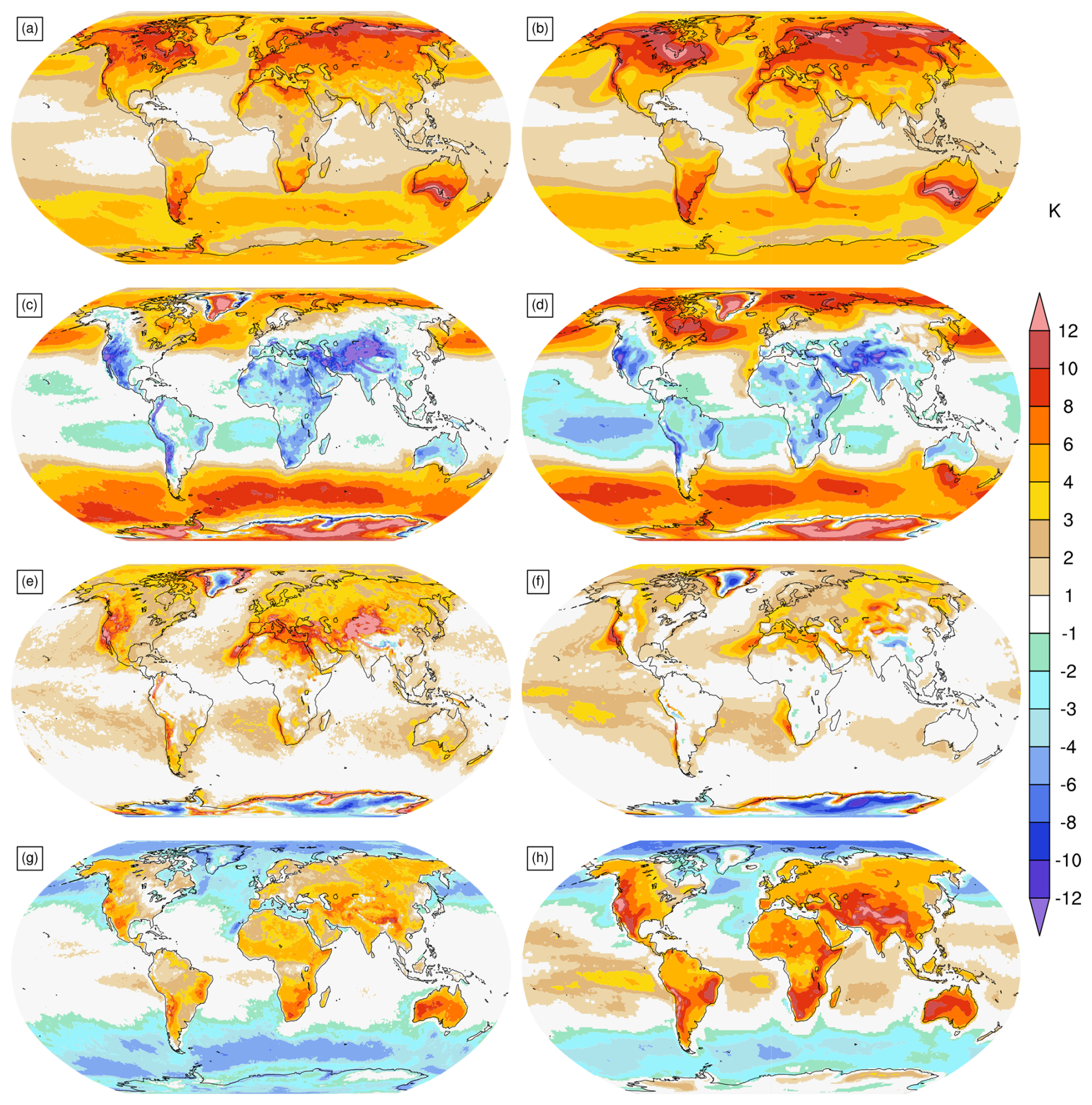
Figure 1 Global TX1day T^′ decomposition for the period 1980–2020 in ERA5 (a, c, e, and g), taken from Röthlisberger and Papritz (2023c), and in CESM2 (b, d, f, and h). Rows show (a, b) the TX1day T^′, (c, d) advective T^′, (e, f) adiabatic T^′ and (g, h) diabatic T^′, respectively.

3 Results

3.1 TX1day anomaly decomposition

We begin by examining global-scale patterns in the TX1day T^′ decomposition in ERA5 and CESM2 (Fig. 1). The qualitative patterns in the TX1day T^′ magnitude largely agree between ERA5 and CESM2 (Fig. 1a, b), with generally more intense TX1day events over land than over ocean and the globally most intense TX1day events over Siberia, Canada, and southern Australia. Also for the advective, adiabatic, and diabatic T^′, the qualitative patterns agree between the two data sets and reveal dominant advective contributions to TX1day events in stormtrack regions, considerable adiabatic contributions over subtropical ocean regions as well as some extratropical land regions, and pronounced diabatic T^′ over most tropical and extratropical land regions in both data sets (Fig. 1c–h).

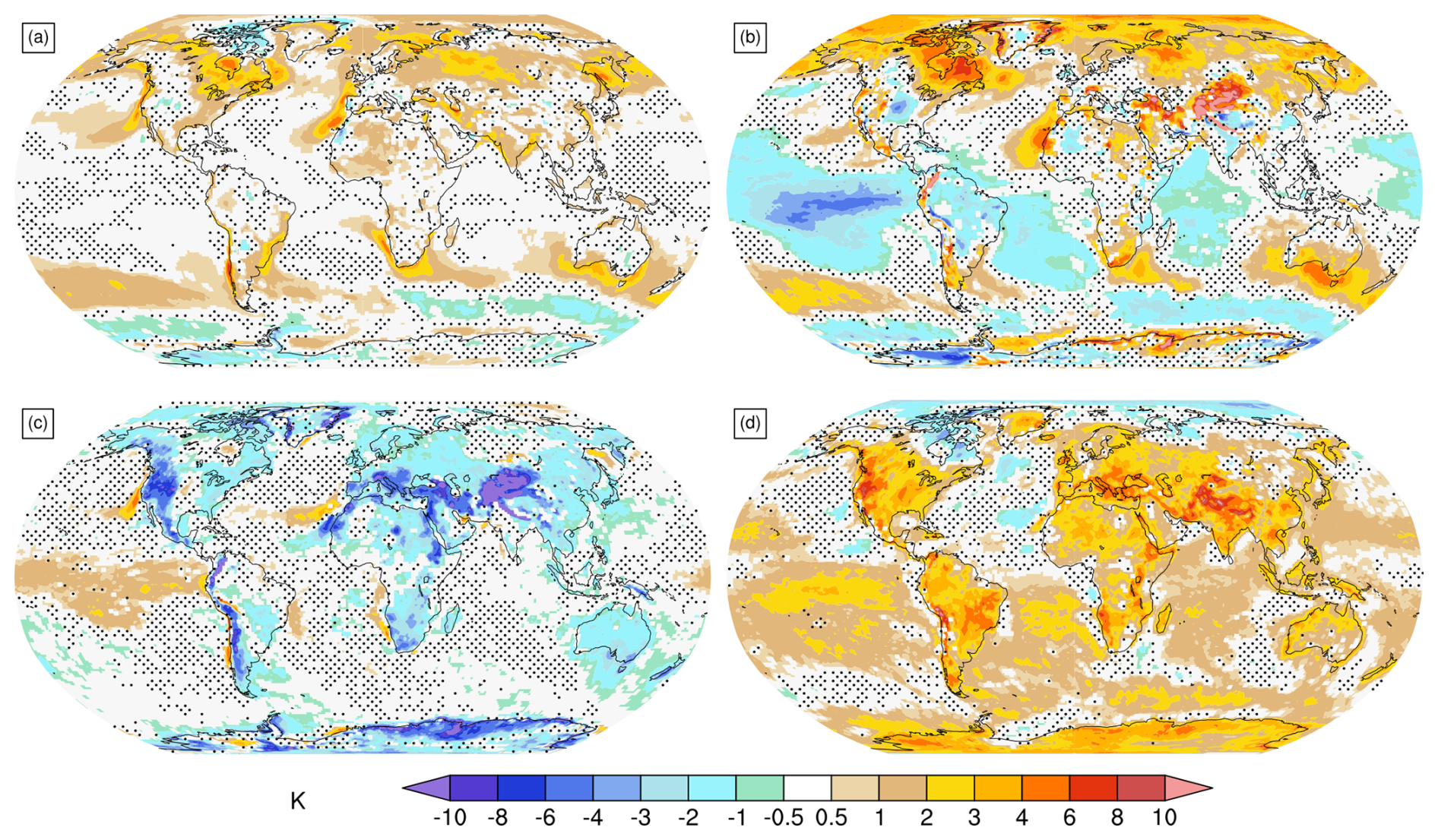
Figure 2 Climatological differences (CESM2 minus ERA5, for period 1980–2020) in TX1day T^′ and its contributions. Panels show (a) ΔT^′, (b) Δ advective T^′, (c) Δ adiabatic T^′, and (d) Δ diabatic T^′. Stippling in all panels indicates that the respective ERA5-value lies within the range of the respective values from the four CESM2 ensemble members.

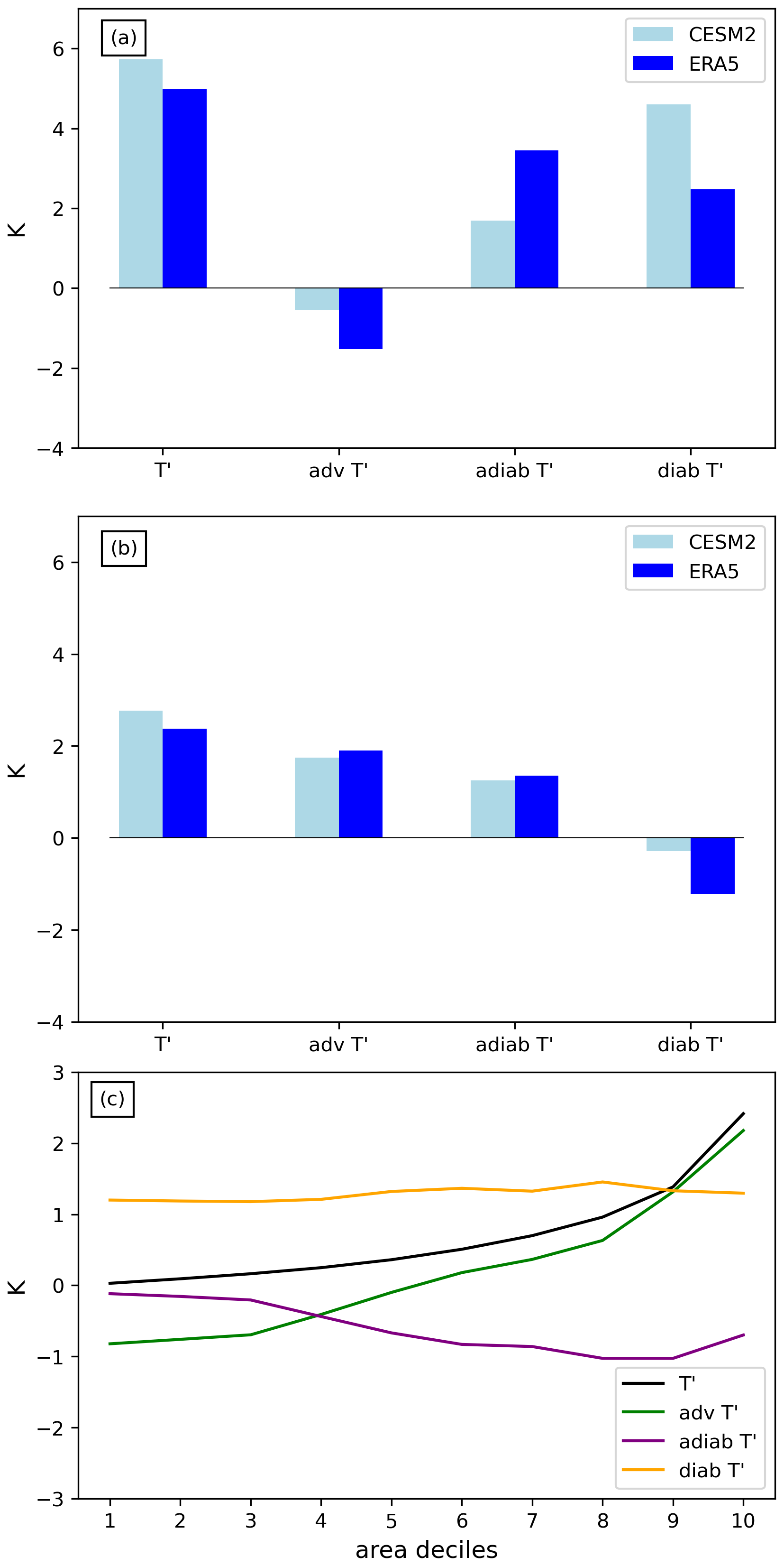
Figure 3 Climatological results for the period 1980–2020 of (a, b) TX1day T^′ decomposition in CESM2 (light blue) and ERA5 (blue) spatially aggregated over (a) land areas below 1500 $\mathrm{m}\mathrm{a}.\mathrm{s}.\mathrm{l}.$ (m above sea level), CESM2 topography) and (b) ocean regions. (c) shows differences (CESM2 minus ERA5) as a function of the magnitude of ΔT^′. All ocean and land grid points below 1500 $\mathrm{m}\mathrm{a}.\mathrm{s}.\mathrm{l}.$ have been binned into ten bins with equal area according to the magnitude of ΔT^′ (area deciles), from (left) the decile with the smallest to (right) the decile with the largest magnitude of ΔT^′. Colored lines depict the differences in TX1day T^′ and its decomposition, averaged for each area decile.

Quantitatively, however, systematic discrepancies in both the magnitude of T^′ and the contributions from the different processes to TX1day T^′ are found across the globe. Averaged globally, TX1day T^′ magnitudes are overestimated in CESM2 by 0.49 K (0.70 K when only considering land regions), while absolute values of the differences in ΔT^′ are smaller than 1 K in 80 % of all regions below 1500 $\mathrm{m}\mathrm{a}.\mathrm{s}.\mathrm{l}.$ (Figs. 2a and 3c), they reach substantial values in some areas. For example, in western Russia and eastern Canada, TX1day T^′ in CESM2 exceeds the respective value in ERA5 by more than 3 K (Fig. 2a). Similarly, substantially more intense TX1day events in CESM2 are found over the eastern North Atlantic and North Pacific, off the coast of Namibia as well as in the seas south of Australia. Negative values of ΔT^′ are far less widespread than positive values; they are prevalent in the Southern Ocean and in few land regions including the western United States (Fig. 2a).

Considering differences between CESM2 and ERA5 in the three contributions to TX1day T^′ over land, they are particularly large for the adiabatic and diabatic T^′ (Figs. 2 and 3a), also in regions where ΔT^′ magnitudes are modest, e.g., in Europe, vast parts of Africa and Australia. Over almost all land regions, the adiabatic T^′ is considerably smaller in CESM2 compared to ERA5 (Fig. 2c). Averaged across all land regions with altitudes below 1500 $\mathrm{m}\mathrm{a}.\mathrm{s}.\mathrm{l}.$ in CESM2, the adiabatic T^′ in CESM2 (1.69 K) is less than half that in ERA5 (3.45 K), while the diabatic T^′ in CESM2 (4.61 K) is much larger than in ERA5 (2.48 K, Fig. 3a). Furthermore, in regions of complex topography, there is poor quantitative agreement between the two datasets regarding the TX1day T^′ composition. This, however, is an expected result, as the topography is less well resolved in CESM2, with significant effects on trajectories of near-surface air parcels.

Also over ocean regions, systematic differences in the TX1day T^′ composition are apparent between the two data sets. Averaged across all ocean regions, CESM2 TX1day events feature −0.29 K diabatic T^′, compared to −1.21 K in ERA5 (Fig. 3b). Furthermore, in several subtropical and tropical ocean regions (in particular the tropical Pacific), there are larger negative advective contributions to CESM2 TX1day events compared to those in ERA5 (Fig. 2b). In the tropical Pacific, the more intense negative advective contributions in CESM2 are offset in part by more positive adiabatic T^′. Note, however, that both the magnitude of TX1day T^′ as well as its difference to ERA5 ΔT^′ is small over tropical ocean regions. Interestingly, advective T^′ is overestimated mainly in regions where the general amplitude of TX1day T^′ is also overestimated (e.g., over eastern Canada and southern Australia; Fig. 2a and b).

Figure 3c, which shows differences of the T^′ composition as a function of the magnitude of ΔT^′, reveals some additional interesting aspects. Consistent with the previous discussion, differences in advective T^′ are positive at the grid points with the largest differences ΔT^′, and they are negative at grid points where ΔT^′ is small. At these grid points the negative differences in advective T^′ is mainly balanced by positive differences in diabatic T^′. Interestingly, the average differences in diabatic T^′ are fairly independent of ΔT^′ (flat orange curve in Fig. 3c). In contrast, the differences in adiabatic T^′ are always negative but strongly increases in magnitude at grid points with larger ΔT^′, compensating the differences in diabatic T^′ at the grid points with the largest values of ΔT^′.

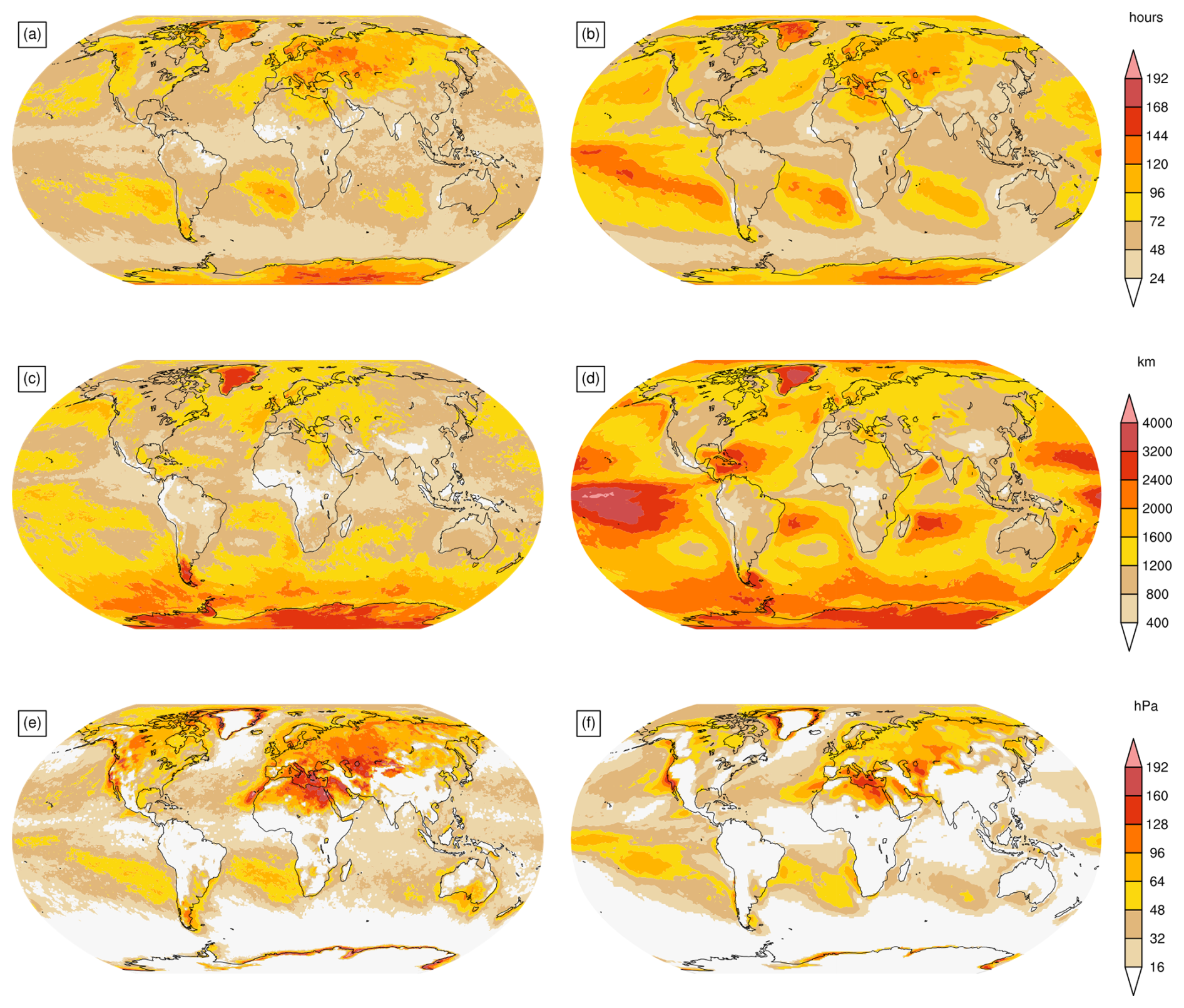
Figure 4 Maps of the TX1day T^′ characteristics: (a, b) age, 𝒜, (c, d) formation distance, 𝒟, and (e, f) vertical displacement, 𝒫 in panels (a), (c), and (e) for ERA5 and (b), (d), and (f) for CESM2.

3.2 Spatiotemporal characteristics of TX1day anomalies

Next we consider the temporal, horizontal, and vertical scales over which near-surface TX1day anomalies form in the two data sets, by examining the Lagrangian characteristics age, 𝒜, formation distance, 𝒟, and vertical displacement since anomaly genesis, 𝒫 (Figs. 4 and 5). The large-scale patterns in 𝒜 and 𝒫 largely agree between the two data sets, in particular for TX1day events over land. Oldest TX1day anomalies are found in both data sets over western Russia, Greenland, and in subtropical anticyclones (Fig. 4a and d). However, in particular for TX1day events in the tropical Pacific, CESM2 substantially overestimates 𝒜 (by up to 4 d, while in ERA5 𝒜 in these regions is typically less than 3 d, Figs. 5a and 4a, b). Nevertheless, over land regions, 𝒜 differences are typically less than 10 h and the spatial patterns in 𝒜 agree remarkably well between the two data sets (Fig. 4a and b). Similarly, also the spatial patterns in 𝒫 agree very well (Fig. 4e and f), with globally largest 𝒫 in the Mediterranean region and around major orography. Quantitatively, however, CESM2 systematically underestimates 𝒫, in particular over land regions (Fig. 5c), as 𝒫 is 40 hPa in ERA5 and only 13 hPa in CESM2 when averaging across all TX1day events occurring at land grid points below 1500 $\mathrm{m}\mathrm{a}.\mathrm{s}.\mathrm{l}.$ in the CESM2 topography. That is, air parcels contributing to TX1day events in CESM2 subside less after anomaly genesis than their counterparts in ERA5, which points to a different combination of physical mechanisms leading to heat extremes in CESM2 compared to ERA5.

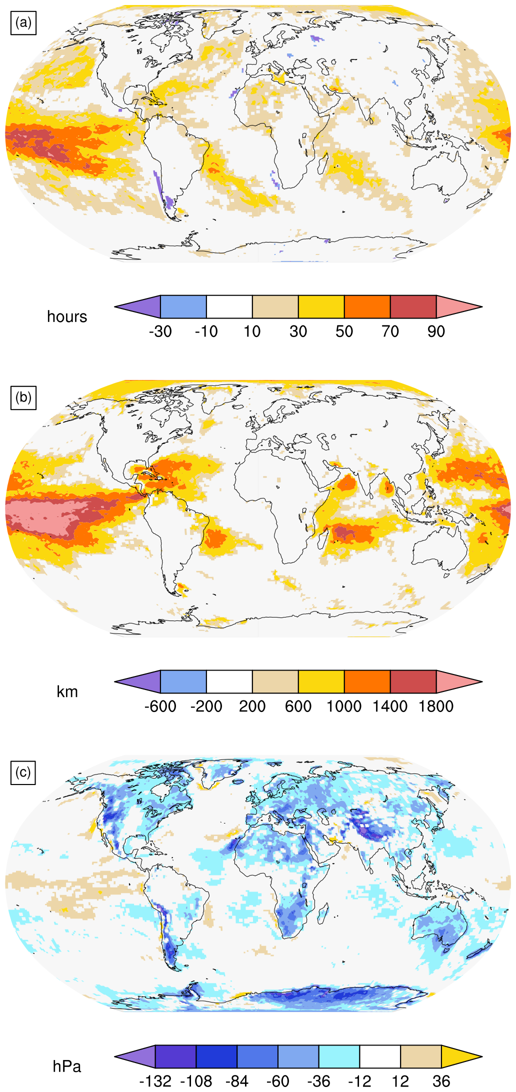
Figure 5 Difference maps (CESM2 minus ERA5) of the TX1day T^′ characteristics: (a) age, 𝒜, (b) formation distance, 𝒟, and (c) vertical displacement, 𝒫.

Furthermore, for the formation distance 𝒟, considerable differences are apparent already in its large-scale patterns (Fig. 4c and d). Over vast tropical and subtropical ocean regions, 𝒟 in CESM2 exceeds 𝒟 in ERA5 by more than 1000 km (Fig. 5b), which in many regions constitutes a difference of more than 100 %. That is, while in ERA5 TX1day T^′ over tropical and subtropical oceans form over hundreds to typically less than 1500 km, the CESM2 TX1day T^′ in the same region form over several thousand kilometers. Hereby, the overestimation in 𝒟 is particularly large for TX1day events in the tropical Pacific, in agreement with the overestimation of the age, 𝒜, in this region (Fig. 5a and b). Clearly, these large discrepancies in the spatiotemporal characteristics of TX1day T^′ over tropical and subtropical oceans are worrying and warrant further investigation. Nevertheless, note that over land regions the patterns of 𝒟 are qualitatively similar in the two data sets, and they even quantitatively rarely differ by more than 250 km. Moreover, over land even comparatively small-scale spatial variations in 𝒟 are often reproduced, e.g., in Spain, where TX1day events feature 𝒟 of less than 1000 km in both data sets, while in Scandinavia 𝒟 typically exceeds 1500 km.

So far our analyses have revealed that (a) CESM2 overestimates the magnitude of TX1day events in many regions, and, moreover, these particular regions feature also larger advective T^′ in CESM2 compared to ERA5. (b) CESM2 systematically overestimates the diabatic contribution and underestimates the adiabatic contribution to TX1day T^′, in particular over land regions. (c) Over land regions, 𝒜 and 𝒟 of TX1day T^′ are comparable between CESM2 and ERA5 (not over oceans, however), while 𝒫 is substantially underestimated in CESM2, which is consistent with the underestimated adiabatic T^′. In the remainder of this paper we focus on the key findings (a) and (b) and further investigate their potential causes.

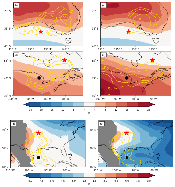
Figure 6 Comparison of $\stackrel{\mathrm{‾}}{T}$ at 900 hPa (shading, relative to the value at the grid point marked by the red star) and genesis location densities for TX1day anomalies (yellow contours with values of 0.01, 0.02, 0.05 and 0.1) between (left) ERA5 and (right) CESM2 in the vicinity of selected grid points, denoted by red stars, at (a, b) 37° S/131° E in the Great Australian Bight, (c, d) 55° N/70.5° W, in eastern Canada, and (e, f) 38° N/95° W in the central US. Genesis location densities denote the fraction of all genesis events of TX1day anomalies at the red star that occur within 200 km radius of the respective grid point. In panels (a) and (b) daily mean T is considered for 1 January and in panels (c)–(f) for 1 July 2000, respectively.

3.3 Differences in TX1day T^′ magnitude and their relation to advective T^′

3.3.1 Example cases

The co-occurrence of large magnitudes of ΔT^′ and Δ advective T^′ in many regions in Fig. 2a and b is striking and suggests that understanding differences in the advective T^′ during TX1day events is key to understanding differences in TX1day magnitude. On a conceptual level, differences in advective T^′ could have two underlying reasons: (1) a “circulation difference conditional to TX1day events” (hereafter shortened to “circulation difference”), i.e., differences in the circulation leading up to TX1day events in CESM2 and ERA5, which would result in different trajectories of air parcels contributing to TX1day events. (2) a “mean-state difference”, i.e., differences in horizontal gradients of the temperature climatology $\stackrel{\mathrm{‾}}{T}$ between CESM2 and ERA5, such as differing climatological land-ocean contrasts or meridional temperature gradients. Such mean state differences would yield differences in advective T^′ even in the absence of any circulation difference. Of course, a combination of (1) and (2) is also plausible, and we should mention that we cannot expect a freely-running climate model to perfectly reproduce the circulation of the 41 considered TX1day events in ERA5. In the following, we examine, based on three example cases as well as a systematic global analysis, to what extent circulation and mean-state differences are relevant for explaining Δ advective T^′ (and thus also ΔT^′).

We first consider the grid point at 37° S/131° E (note that whenever we refer to a location specified with latitude and longitude values we mean the grid point closest to that location in either dataset), in the Great Australian Bight, where the advective T^′ is 9.36 K in CESM2 and 5.04 K in ERA5. Figure 6a and b reveals that this difference is largely due to a circulation difference. The spatial distribution of the genesis locations of TX1day T^′ differs considerably between the two data sets and a sizable fraction of air parcels contributing to TX1day events in ERA5 approaches 37° S/131° E from the west (Fig. 6b), while in CESM2 TX1day air parcels almost exclusively approach 37° S/131° E from the northeast, i.e., from the Australian continent (Fig. 6a). Moreover, the $\stackrel{\mathrm{‾}}{T}$ gradients at 900 hPa (where in both data sets the respective air parcels acquire their T^′, see Fig. 4e and f) are nearly identical between CESM2 and ERA5 (Fig. 6a and b) and their difference thus cannot contribute considerably to Δ advective T^′ in this region.

A different picture emerges when examining 900 hPa $\stackrel{\mathrm{‾}}{T}$ and genesis locations of TX1day T^′ at 55° N/70.5° W, in eastern Canada (Fig. 6c and d). There, the advective T^′ in CESM2 and ERA5 are, respectively, 11.07 and 4.47 K. Differences in the spatial distribution of the respective TX1day T^′ genesis locations hint to some circulation differences conditional on TX1day events, with more genesis locations further southwest in CESM2 compared to ERA5. However, a further striking difference is found in the near-surface $\stackrel{\mathrm{‾}}{T}$ field. In particular, far stronger northeast to southwest gradients are found in CESM2 compared to ERA5 (resulting from a climatologically warmer central North America in CESM2 compared to ERA5 at that pressure level). This difference in gradients implies that even in absence of any circulation differences, much larger advective contributions result in CESM2 compared to ERA5. For instance, if an air parcel moved isobarically on 900 hPa from 45° N/85° W (the black circle in Fig. 6c and d) to 55° N/70.5° W, it would acquire 14.62 K advective T^′ in CESM2 but only 7.53 K in ERA5. That is, at 55° N/70.5° W both circulation and mean-state differences contribute to Δ advective T^′.

Finally, at 38° N/95° W, in the central US, Δ advective T^′ is related almost exclusively to differences in $\stackrel{\mathrm{‾}}{T}$ (Fig. 6e and f), i.e., to a large mean-state difference. There, the advective T^′ is −3.93 K in CESM2 and −0.45 K in ERA5. In both datasets the bulk of the TX1day T^′ values have their genesis in the area of 28–38° N/95°–103° W, and thus air contributing to TX1day events approach 38° N/95° W from almost exactly the same regions in both data sets. However, at near-surface levels (where these T^′ form, see also Fig. 4e and f), $\stackrel{\mathrm{‾}}{T}$ substantially differs between the two data sets (Fig. 6e and f), again resulting from the climatological warmer central North America in CESM2 compared to ERA5. Consequently, an air parcel moving isobarically on 900 hPa from 25° N/95° W (the black circle in Fig. 6e and f) to 38° N/95° W would acquire an advective T^′ of roughly −5.38 K in CESM2 but only −0.25 K in ERA5. The grid point at 38° N/95° W thus illustrates that considerable differences in the advective T^′ can occur despite TX1day air parcels approaching the respective location from a very similar region in the two data sets.

These three examples illustrate qualitatively that both circulation and mean-state differences can contribute to differences in advective T^′ at individual grid points. How large these contributions to Δ advective T^′ are at a global scale is explored in the next section.

3.3.2 A systematic quantification of contributions of circulation and mean state differences on differences in advective T^′

The following analysis is technically the most involved of this study, and requires careful explanations. Quantifying the contributions of the circulation and mean-state differences to Δ advective T^′ can be achieved by first interpolating ${\stackrel{\mathrm{‾}}{T}}_{\text{ERA5}}$ to the CESM2 grid (as detailed in Appendix B), and, second, tracing the interpolated ${\stackrel{\mathrm{‾}}{T}}_{\text{ERA5}}$ (hereafter referred to as ${\stackrel{\mathrm{‾}}{T}}_{\text{ERA5}}^{\ast }$) along CESM2 TX1day trajectories. The basic idea behind this is to investigate the resulting temperature anomalies when considering the CESM2 trajectories moving through the ERA5 temperature climatology. Knowledge of the values of ${\stackrel{\mathrm{‾}}{T}}_{\text{ERA5}}^{\ast }$ along these trajectories then allows computing the advective T^′ acquired by a CESM2 trajectory between its t_g (defined based on ${\stackrel{\mathrm{‾}}{T}}_{\text{CESM2}}$) and t_X relative to the (interpolated) ERA5 climatology ${\stackrel{\mathrm{‾}}{T}}_{\text{ERA5}}^{\ast }$. This quantity corresponds to the advective T^′ a CESM trajectory would have in the $\stackrel{\mathrm{‾}}{T}$ field of ERA5, and is hereafter referred to as advective $T^{\prime \ast }$, and formally defined as

$$\begin{array}{}\text{(2)}& \text{advective}{T}^{\prime \ast }=-\underset{t_{\mathrm{g}}}{\overset{t_X}{\int }}\mathbf{v}\cdot {\mathrm{\nabla }}_{\mathrm{h}}{\stackrel{\mathrm{‾}}{T}}_{\text{ERA5}}^{\ast }\mathrm{d}\mathit{\tau },\end{array}$$

analogously to the advective T^′ (see second term on the r.h.s of Eq. 1). Upon introducing advective $T^{\prime \ast }$, the expression for Δ advective T^′ can be rewritten as

$$\begin{array}{}\text{(3)}& \begin{array}{rl}\mathrm{\Delta }\text{advective}{T}^{\prime }& =\left(\text{advective}{T}_{\text{CESM2}}^{\prime }-\text{advective}{T}^{\prime \ast }\right)\\ & +\left(\text{advective}{T}^{\prime \ast }-\text{advective}{T}_{\text{ERA5}}^{\prime }\right),\end{array}\end{array}$$

whereby advective $T_{\text{CESM2}}^{\prime }$ and advective $T_{\text{ERA5}}^{\prime }$ denote the advective T^′ computed in either data set in the standard way, i.e., the fields depicted in Fig. 1c and d. Note that the first bracket on the r.h.s. of Eq. (3) denotes the difference in advective T^′ that results for CESM2 trajectories when computing advective T^′ with either temperature climatology. This term thus quantifies the effect of differences in horizontal gradients of $\stackrel{\mathrm{‾}}{T}$ between CESM2 and ERA5 on the resulting advective T^′, and is hereafter referred to as “mean state difference” term. Conversely, the second bracket denotes the difference in advective T^′ (computed relative to the ERA5 climatology) that arises when considering CESM2 trajectories (advective $T^{\prime \ast }$) as opposed to ERA5 trajectories (advective $T_{\text{ERA5}}^{\prime }$). This term thus quantifies the effects of circulation differences (i.e., differing trajectories) on advective T^′ and is hereafter referred to as “circulation difference” term.¹

The resulting advective $T^{\prime \ast }$ as well as the mean-state and circulation differences are shown in Fig. 7. The large-scale patterns in advective $T^{\prime \ast }$ strongly resemble those of advective T^′ for CESM2 or ERA5 (compare Figs. 7a and 1c, d). This is an expected result given the similarity of the large-scale patterns in advective T^′ in these two data sets. Yet, quantitatively, advective $T^{\prime \ast }$ differs from advective T^′ in either data sets, which leads to non-zero mean-state and circulation differences in Fig. 7b and c. The mean-state difference term (Fig. 7b) features local peaks exceeding 3 K for TX1day events in eastern Canada and lowest values below −3 K in the Southern Ocean. Consistent with the detailed analysis for the grid point at 55° N/70.5° W (eastern Canada, Fig. 6c and d), CESM2 trajectories for TX1day events in eastern Canada acquire far more advective T^′ relative to ${\stackrel{\mathrm{‾}}{T}}_{\text{CESM2}}$ than relative to ${\stackrel{\mathrm{‾}}{T}}_{\text{ERA5}}^{\ast }$. In particular over most land regions, however, the mean-state term is typically less than 1 K. Also, averaged over all land regions below 1500 $\mathrm{m}\mathrm{a}.\mathrm{s}.\mathrm{l}.$, the mean state term is 0.11 K.

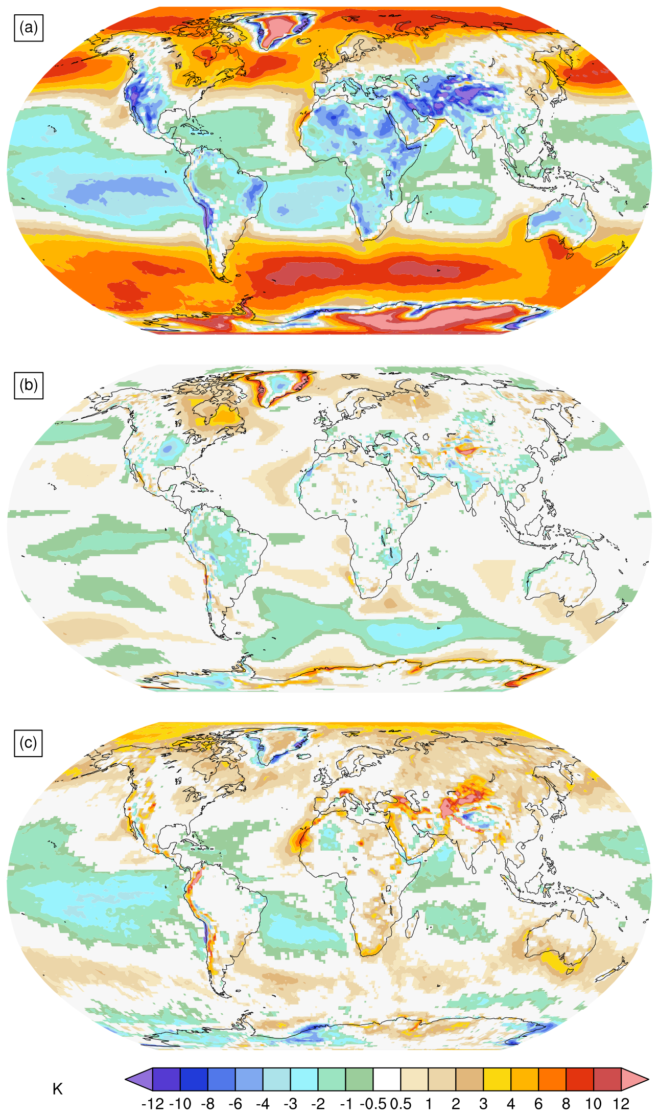
Figure 7 (a) Advective $T^{\prime \ast }$, (b) the mean state term (advective $T_{\text{CESM2}}^{\prime }$ – advective $T^{\prime \ast })$, and (c) the circulation term (advective $T^{\prime \ast }$ – advective $T_{\text{ERA5}}^{\prime })$. See text for details.

The circulation difference also features large spatial variability, with peak magnitudes in excess of 5 K even away from major orography and large areas of negative values over tropical oceans (Fig. 7c). Over land, however, the circulation difference is mostly positive and amounts to 0.88 K when averaging over all land regions below 1500 $\mathrm{m}\mathrm{a}.\mathrm{s}.\mathrm{l}.$ That is, the overestimation of the advective T^′ in CESM2 over land (and likely related to that the overestimation of TX1day T^′) is predominantly due to circulation differences associated with TX1day events rather than differences in the background $\stackrel{\mathrm{‾}}{T}$ fields (Fig. 7b and c).

In summary, the analyses illustrated in Figs. 6 and 7 imply that at a regional scale, both differences between CESM2 and ERA5 in $\stackrel{\mathrm{‾}}{T}$ (i.e., mean-state differences) as well as in the circulation can contribute to the differences in advective T^′. In particular in eastern Canada, where both ΔT^′ and Δ advective T^′ are large (Fig. 2a and b), the mean-state term contributes significantly to Δ advective T^′, and thus also to ΔT^′. However, in most other land regions with large ΔT^′, circulation differences appear to be key for explaining large values of Δ advective T^′. Given the frequent co-occurrence of positive ΔT^′ and positive Δ advective T^′, we thus conclude that circulation differences conditional to TX1day occurrence are key to explaining the widespread overestimation of the TX1day magnitude in CESM2.

3.4 Differences in adiabatic T^′ and diabatic T^′

Next, we focus on the differences in the physical mechanisms during TX1day events in CESM2, and examine potential causes of Δ adiabatic T^′ and Δ diabatic T^′. Specifically, we examine two hypotheses: (a) the differences in adiabatic and diabatic T^′ could result from resolution differences between the two data sets (assuming that the resolution of the wind fields impacts the trajectories' (vertical) motion); (b) the overestimation of diabatic T^′ in CESM2 is related to a different partitioning of heat fluxes (i.e., stronger sensible and weaker latent heat fluxes) during and preceding TX1day events in CESM2 compared to ERA5, as suggested for other models in previous studies (e.g., Mueller and Seneviratne, 2014; Wehrli et al., 2018).

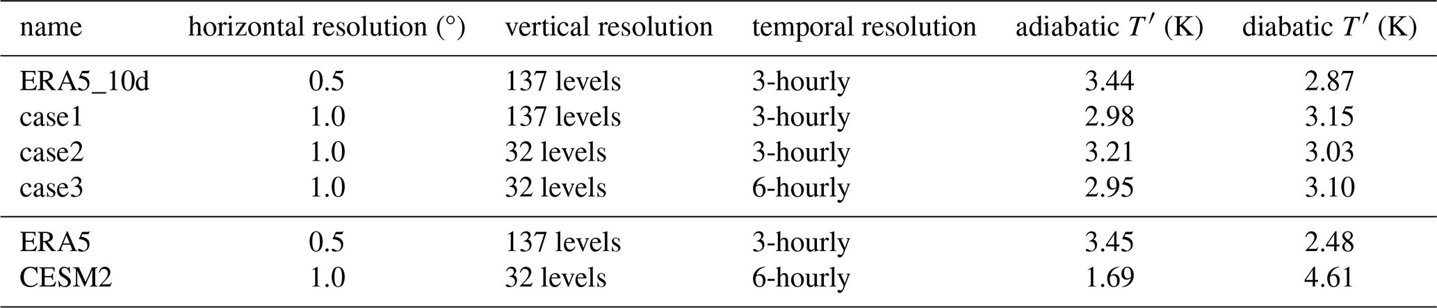
Table 1 Key characteristics of interpolation experiments. The fifth and sixth column denote the adiabatic and diabatic T^′ in each experiment averaged across all land areas below 1500 $\mathrm{m}\mathrm{a}.\mathrm{s}.\mathrm{l}.$, respectively. The experiments in the first four rows considered the decomposition of near-surface T^′ during the 5 hottest days at each grid point in the years 2020 and 2021, while the last two rows correspond to the standard analyses in this study, i.e., to the results displayed in Fig. 1.

3.4.1 Resolution dependence

Recall that the two data sets (as used here) feature the following spatial and temporal resolutions: in the horizontal 0.5° in ERA5 vs. approximately 1° in CESM2, in the vertical 137 levels in ERA5 vs. 32 in CESM2, and temporally 3 h in ERA5 vs. 6 h in CESM2. Such resolution differences could affect our results in two ways. Firstly, there could be purely kinematic effects on the computation of trajectories. That is, trajectories computed from one single data set (e.g., ERA5) but with input wind fields at different resolutions most likely differ. If such kinematic effects were large, they would to some degree compromise the interpretability of results obtained from the Lagrangian T^′ decomposition, as the results would then depend on the resolution of the input data rather than the physical mechanisms of the analysed events. Secondly, differences in the native resolution between different data sets could entail that certain processes are better resolved in one data set, while they are less adequately resolved in the other. Such differences in model physics and numerics too could result in differences in advective, adiabatic, and diabatic T^′. These differences, however, directly result from model deficiencies rather than the method to identify them (i.e., the Lagrangian T^′ decomposition) and can hence be considered as “model biases”.

In the following we perform several interpolation experiments, where we first interpolate ERA5 data to different horizontal, vertical, and temporal resolutions, then re-calculate the backward trajectories with the interpolated fields, and finally use the Lagrangian T^′ decomposition to decompose the same near-surface T^′ in each of the interpolated data sets. For computational reasons, these experiments were restricted to 2 randomly selected years in ERA5 (2020 and 2021), and instead of considering TX1day events only, the 5 hottest days at each grid point based on daily mean T2m were selected, which yields 10 events at each grid point (compared to two if only selecting TX1day events). Differences between re-gridded versions of ERA5 are then interpreted as the above mentioned “kinematic effects” (same model, different resolution), while the “remaining differences” are considered as model biases due to unresolved processes.

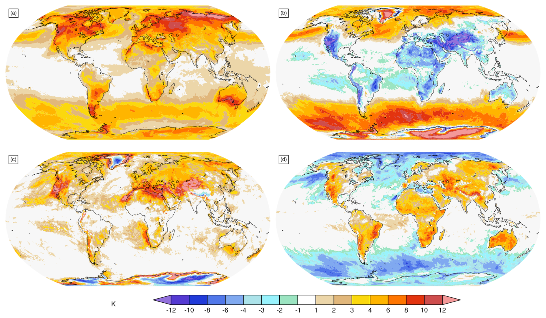
Figure 8 Results for the ERA5_10d experiment (see text for details), showing (a) T^′ and its (b) advective, (c) adiabatic, and (d) diabatic components.

Specifically, we perform the following experiments, whose key characteristics are detailed in Table 1: Analogously to the TX1day T^′ decomposition, we first decompose near-surface T^′ during the 10 selected hot days at each grid point, using the standard ERA5 fields. This experiment is hereafter referred to as ERA5_10d and serves as control experiment for the experiment detailed below. The results of the ERA5_10d experiment are shown in Fig. 8, which reveals that near-surface T^′ during the considered days in 2020 and 2021 broadly feature similar characteristics as the TX1day anomalies (identified over 41 years) shown in Fig. 1 (albeit with slightly smaller T^′ in most regions, and more noisy fields, since fewer and less extreme events are considered).

Next we interpolate the 2020 and 2021 ERA5 data horizontally to a resolution of 1°, while retaining the full vertical resolution and the three-hourly temporal resolution. This dataset will be referred to as case 1. Next, the fields from case 1 are vertically interpolated to 32 levels, while again retaining the three-hourly temporal resolution (case 2), and finally these fields are additionally temporally restricted to the 6-hourly values (case 3). For all cases we repeat the decomposition of the respective near-surface T^′ during the 10 hot events at each grid point, yielding fields analogous to those shown in Fig. 8 for each experiment.

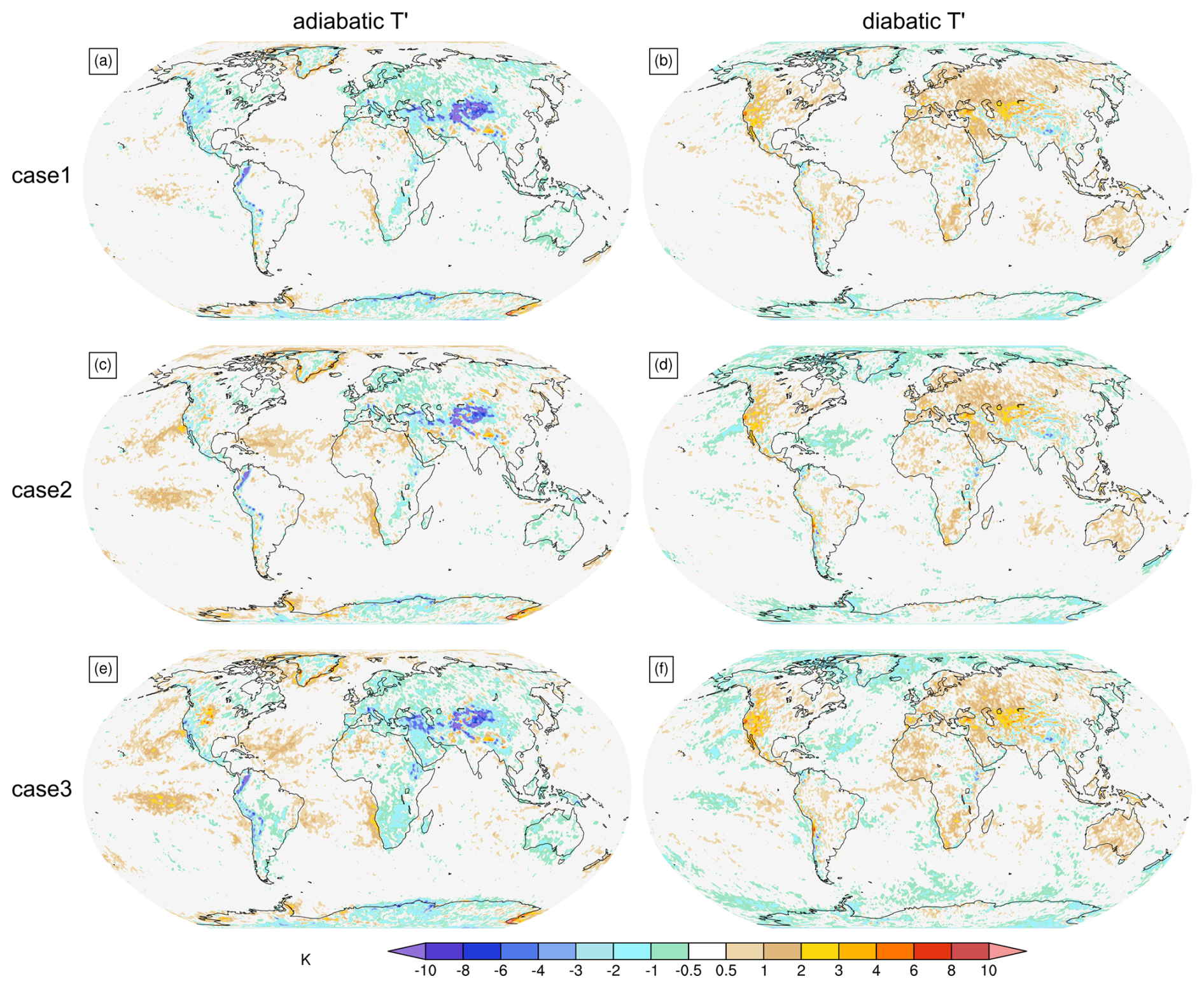
Figure 9 Differences of (a, c, e) adiabatic T^′ and (b, d, f) diabatic T^′ between the three cases and ERA5_10d for near-surface T^′ during the hottest 5 d in 2020 and 2021 at each grid point. The rows depict the three resolution modification cases as indicated, the respective resolution modifications are detailed in Table 1.

Differences in the adiabatic and diabatic T^′ between the three cases and ERA5_10d are shown in Fig. 9 and Table 1 (differences are taken as, e.g., case 1 minus ERA5_10d, etc.). They reveal that indeed there is some resolution dependence of the Lagrangian T^′ decomposition, which explains some of the differences detailed in Fig. 2. Over land regions, the adiabatic T^′ is smaller for all three cases than for ERA5_10d (largest difference of 0.49 K for case 3, when averaging over land areas below 1500 $\mathrm{m}\mathrm{a}.\mathrm{s}.\mathrm{l}.$, Table 1), while the diabatic T^′ is somewhat larger (largest difference of 0.28 K for case 1). Moreover, there are large differences near major orography, as one might expect (Fig. 9). However, the magnitude of these differences is considerably smaller than the ones depicted in Fig. 2. When averaging over all land regions below 1500 $\mathrm{m}\mathrm{a}.\mathrm{s}.\mathrm{l}.$, Δ adiabatic T^′ and Δ diabatic T^′ are −1.77 and 2.13 K, while the magnitude of the difference in adiabatic T^′ between the three cases and ERA5_10d is less than 0.5 K for adiabatic T^′ and less than 0.3 K for diabatic T^′ (Table 1). Thus, at least away from high topography, the resolution dependence does not explain the bulk of the differences in Fig. 2. Consequently, these differences in adiabatic and diabatic T^′ have to be mainly interpreted as differences in the physical mechanisms leading to TX1day events in ERA5 and CESM2.

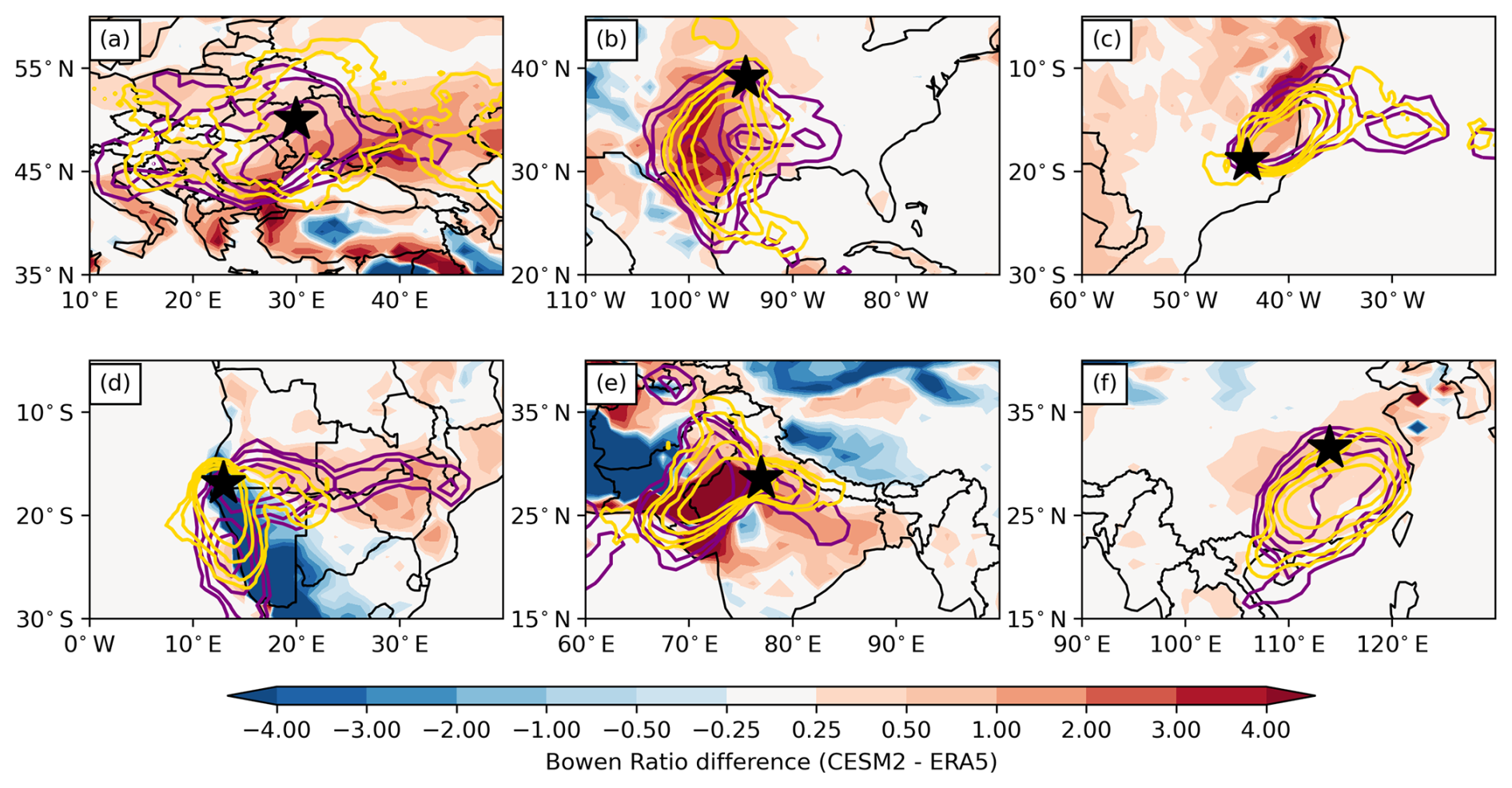
Figure 10 Shading depict differences in the mean Bowen ratio averaged for all TX1day events at the location indicated with the black star. Red colors (i.e., larger Bowen ratios in CESM2 compared to ERA5) indicate a heat flux partitioning with more dominant sensible and attenuated latent heat fluxes during TX1day events in CESM2. Purple and yellow contours depict genesis densities of TX1day anomalies in CESM2 and ERA5, respectively, in the same units as in Fig. 6. Black stars denote the locations of (a) Kyiv, Ukraine, (b) Kansas City, United States, (c) Belo Horizonte, Brazil, (d) the Epupa Falls, at the border between Namibia and Angola, (e) Delhi, India, and (f) Wuhan, China.

3.4.2 Heat flux partitioning during heat extremes

Inspired by Wehrli et al. (2018), we next examine whether differences in the heat flux partitioning in CESM2 might explain differences in diabatic T^′. To this end, we select grid points in regions with particularly large Δ diabatic T^′ and compute the mean Bowen ratio (i.e., sensible heat fluxes divided by latent heat fluxes) during the TX1day events at these grid points in CESM2 and ERA5, respectively. Bowen ratio differences (CESM2 minus ERA5) are shown in Fig. 10. As a caveat we should note here that surface fluxes are most likely also not unbiased in ERA5, as they are poorly constrained by observations and therefore the data assimilation procedure (Muñoz-Sabater et al., 2021).

We first examine the grid point near Kyiv, Ukraine (Fig. 10a), where the diabatic T^′ in CESM2 and ERA5 is 6.1 and 1.9 K, respectively. During TX1day events there, essentially all of eastern Europe features larger Bowen ratios in CESM2 than in ERA5, implying more dominant sensible and attenuated latent heat fluxes in CESM2 compared to ERA5. At numerous grid points in Europe, the overestimation and underestimation of sensible and latent heat fluxes (we pretend here that ERA5 values are closer to reality – see caveat mentioned above), respectively, exceeds 50 % of the respective ERA5 values (not shown). Given that the formation of the respective TX1day T^′ occurs in eastern Europe (see contours of genesis densities in Fig. 10a), these results strongly suggest that differences in the diabatic contributions to TX1day T^′ in Kyiv are related to differences in the partitioning of heat fluxes, i.e., too little evapotranspiration in CESM2 compared to ERA5, potentially related to too dry soils. A similar picture emerges for TX1day events in Kansas City (Fig. 10b), Belo Horizonte, Brazil (Fig. 10c), Delhi (Fig. 10e), and Wuhan (Fig. 10f). During heat extremes at all these locations, more intense sensible heat fluxes and reduced latent heat fluxes in CESM2 compared to ERA5 are observed in widespread regions around the respective location.

A different, inconclusive picture emerges for TX1day events at the grid point nearest to the Epupa Falls, at the border between Namibia and Angola (Fig. 10d). There, the Bowen ratio difference is negative, and the “source regions” of TX1day T^′ seem to differ considerably between CESM2 and ERA5, and cover regions with Bowen ratio differences of either sign.

Evidently, the degree to which these case study results can be generalized needs to be evaluated further. However, as we have selected the grid points based on the magnitude of Δ diabatic T^′, the analyses presented in Fig. 10 show that at least some of the globally largest diabatic T^′ differences are likely related to a different partitioning of heat fluxes in the source regions of air contributing to TX1day events in the respective regions.

4 Discussion, summary and conclusions

4.1 Discussion

The differences in the magnitude and physical mechanisms leading to heat extremes in CESM2 identified in this study relate to several known deficiencies in current climate models: Positive biases in the magnitude of simulated heat extremes have been documented previously for CMIP5 and 6 models (Wehner et al., 2020; Hirsch et al., 2021; Li et al., 2021). However, the spatial patterns of these biases considerably differ depending on the model (compare Fig. 2a in this study with Fig. 1h in Hirsch et al., 2021), and depending on whether the heat extreme magnitude is quantified with absolute values or anomalies (Wehner et al., 2020; Li et al., 2021). Here we find that differences in TX1day magnitude between CESM2 and ERA5 are related to differences in the circulation conditional to TX1day events, at least when aggregating over all land regions below 1500 $\mathrm{m}\mathrm{a}.\mathrm{s}.\mathrm{l}.$ Subsequent studies should thus assess whether this is also the case for other climate models and, if so, examine in detail the flow features within which heat extremes form in regions of overestimated heat extreme magnitude.

Importantly, however, the differences in the TX1day T^′ magnitude are far smaller (15 % when considering all land regions below 1500 $\mathrm{m}\mathrm{a}.\mathrm{s}.\mathrm{l}.$) compared to differences in the composition of their respective T^′ (−51 % for adiabatic T^′ and +86 % for diabatic T^′ in the same region). Rather worryingly, our results thus suggest that CESM2 reproduces the magnitude of TX1day T^′ rather well, however, the relative contributions of physical mechanisms are strongly biased compared to ERA5 and thus the TX1day events partly occur for the wrong reasons – at least in several land regions.

This may have implications for the robustness of heat extreme projections under future warming. For instance, in regions of large Δ diabatic T^′, intensifying land–atmosphere interactions (Mueller and Seneviratne, 2014; Sippel et al., 2017) could affect simulated heat extremes more strongly than in reality, yielding erroneous projections of heat extremes under global warming. However, such effects would likely also depend on the (observed and simulated) base state regarding soil moisture, as further drying in already too dry regions may be underestimated in simulations (Ficklin et al., 2016). Likewise, projected changes in atmospheric blocking (which are currently rather uncertain) and, related to that, changes in subsidence warming might have little effect on changes in simulated heat extremes under global warming, due to the widespread underestimation of adiabatic T^′ over most land regions. Evidently, the results of this study should be considered when pondering about changes in heat extremes under global warming, in particular if they are related to intensifying land–atmosphere interactions (e.g., Sato and Nakamura, 2019), or changes in blocking (Woollings et al., 2018).

Furthermore, very large differences between CESM2 and ERA5 were found for TX1day events over tropical and subtropical oceans in terms of the Lagrangian age, 𝒜, and the formation distance, 𝒟, of the respective temperature anomalies. While the magnitude of TX1day events is modest in these regions, these differences are still worrying, as they point to a rather different physical mechanism leading to TX1day events in CESM2 compared to ERA5 in these regions. Specifically, these differences imply that in CESM2 anomalously warm air (which later contributes to TX1day events) is transported over longer distances and time periods than in ERA5. Various factors could contribute to such differences, for instance too strong trade winds (Simpson et al., 2018), or an erroneous representation of low clouds, which affects the surface radiation budget in these regions (Richter, 2015). We note that these results about oceanic TX1day events do not necessarily translate to the process relevant for marine heat waves. Given the much longer timescale of these heat waves, potential model biases associated with their occurrence would need to be studied separately.

Moreover, the analyses presented here suffer from at least three caveats, which should be considered when interpreting our results. Firstly, the analyses presented in Fig. 10 hint to one cause of the considerable Δ diabatic T^′, but do not quantify the effect of a potentially biased partitioning of sensible and latent heat fluxes during heat extremes. Subsequent studies could attempt to further decompose the diabatic T^′, e.g., by considering heating tendencies from ERA5 and climate models along air parcel trajectories, as has been done in Attinger et al. (2019) for one specific numerical weather prediction model. Such even more detailed Lagrangian analyses could further pinpoint the physical causes of the considerable Δ diabatic T^′ found in this study. Secondly, we performed analyses with only one model, which prevents making any general statements about the physical mechanisms leading to heat extremes in state-of-the-art models. Clearly, our analyses should be repeated in subsequent studies with various models. However, such analyses are currently severely hampered by the lack of publicly available high-frequency and vertically complete climate model data, which is a prerequisite for computing air parcel trajectories needed for our Lagrangian decomposition of T^′. We thus urge the climate modeling community to provide such high-frequency (at least six-hourly output) and vertically complete data (i.e., from all model levels) for at least a few decades of simulations per model (e.g., one member covering the last few decades), such that our analyses could be repeated with other models and that a more robust understanding could be established of the capability of climate models in simulating the physics of heat extremes. Thirdly, We acknowledge that with the approach of Röthlisberger and Papritz (2023c) we cannot exclude the possibility that some of the differences we identify for TX1day events also emerge when comparing CESM2 and ERA5 mean circulation and heat fluxes (i.e., differences might not be specific to TX1day events). Yet, for addressing the question “Do heat extremes in CESM2 form for the right physical reasons?” it is important to unravel the full biases in the functioning of heat extremes.

Finally, we mention that an alternative Lagrangian approach to decompose temperature anomalies during heat extremes into advective, adiabatic and diabatic components has recently been proposed by Mayer (2025), who found that “horizontal transport is attributed the primary role for heat extremes globally”. At first sight, this finding contrasts Fig. 1 and the results of Röthlisberger and Papritz (2023c). However, in our view, this contrast emerges from the fact that the two studies, Röthlisberger and Papritz (2023c) and Mayer (2025), addressed slightly different research questions: Recall that Röthlisberger and Papritz (2023c) assessed whether temperature anomalies contributing to heat extremes at a particular location X form because (a) air from a climatologically warmer region reaches location X, (b) because air subsides prior to the heat extreme, or (c) because that air is heated diabatically. In some contrast, Mayer (2025) compared the Lagrangian characteristics of air contributing to heat extremes at a location X to Lagrangian characteristics of “climatological” air at location X. Thereby, they construct their “Lagrangian climatology” from air parcels with any temperature anomaly (hot and cold). That is, they assess how anomalous the horizontal transport, adiabatic warming or cooling, and diabatic heating or cooling is compared to climatological air (see Sect. 4 in Mayer, 2025). Evidently, their research question differs from that of Röthlisberger and Papritz (2023c).

Nevertheless, we do note that the finding of Mayer (2025) that “horizontal transport is attributed the primary role for heat extremes globally” contrasts a vast body of literature that highlights the key role for the formation of heat extremes of adiabatic warming (e.g., Fink et al., 2004; Black et al., 2004; Bieli et al., 2015; Sousa et al., 2018; Schumacher et al., 2022; Hotz et al., 2024) and of diabatic warming (e.g., Fischer et al., 2007a; Seneviratne et al., 2010; Miralles et al., 2014, 2019). We propose that the seeming unimportance of adiabatic and diabatic warming for heat extremes in the analyses of Mayer (2025) might be a consequence of the definition of their “Lagrangian climatology”. Recall that Mayer (2025) compared adiabatic warming of air parcels contributing to heat extremes (i.e., anomalously warm air) with the adiabatic warming of all air parcels arriving at a certain location, including often anomalously cold airstreams like dry intrusions (Raveh-Rubin, 2017), which for buoyancy reasons are expected to subside more strongly than anomalously hot air. Nevertheless, this does not exclude the possibility that (the comparatively modest) subsidence warming of already anomalously warm air in an anticyclone might be key to the formation of near-surface heat. Similarly, sensible heating of near-surface air is strongly influenced by the temperature contrast between near-surface air and the Earth's surface. The larger that contrast, the larger the heating/cooling (heating rates far larger than those contributing to heat extremes are observed, for instance, during cold air outbreaks over warm ocean surfaces, e.g., Papritz and Spengler, 2017). Therefore, diabatic heating of already anomalously hot air through sensible heat fluxes from the surface is unlikely to be large compared to that of climatological or anomalously cold air. This, however, again does not render the diabatic heating of anomalously warm air unimportant for near-surface heat. Again, the choice of “Lagrangian climatology” by Mayer (2025) likely explains the contrast between their result (diabatic heating is largely unimportant for heat extremes, their Fig. 3c) with the results of previous studies suggesting the opposite (e.g., Fischer et al., 2007a; Seneviratne et al., 2010; Miralles et al., 2014, 2019).

4.2 Summary

In this study the physical mechanisms leading to heat extremes simulated with CESM2 are evaluated, by comparing near-surface T^′ during TX1day events. In a four-member CMIP-type CESM2 simulation as well as in ERA5, the T^′ is decomposed into its advective, adiabatic, and diabatic contributions, as computed in Röthlisberger and Papritz (2023c). This comparison reveals a good qualitative agreement in the large-scale patterns of TX1day T^′ and its contributions: (i) In both datasets we find more intense TX1day events over land (peak intensities in western North America and Russia exceeding 10 K) than over ocean (least intense TX1day events over tropical and subtropical oceans, with lowest TX1day T^′ magnitudes of less than 1 K); (ii) advective contributions dominate the TX1day T^′ over extratropical storm track regions, where in both data sets air moves poleward on near-surface levels before approaching the respective heat extreme location; (iii) in both data sets, adiabatic T^′ is large for TX1day events in the regions of the climatological subtropical anticyclones, as well as over northern hemispheric extratropical land regions; and (iv) diabatic T^′ is generally positive over land and small or negative over oceans in both data sets, and in both data sets particularly large in subtropical dry regions, such as Australia.

Quantitatively, however, there are large discrepancies between the datasets regarding the advective, adiabatic, and diabatic contributions to TX1day T^′, and, moreover, CESM2 overestimates the magnitude of TX1day T^′ in numerous regions, in particular in the mid-latitudes (averaged globally, the difference in Δ TX1day T^′ is 0.49 K, which is 15 % of the global average of TX1day T^′ in ERA5). Interestingly, regions with large differences in TX1day T^′ also feature large (and same-signed) differences in the advective T^′, suggesting a tight relationship between the two. Detailed analyses of the underlying causes for the differences in advective T^′ reveal that at a regional scale, differences in circulation leading to the TX1day events (i.e., differences in the air parcel trajectories) and differing horizontal gradients of $\stackrel{\mathrm{‾}}{T}$ contribute both to the differences in advective T^′, albeit with larger contributions from circulation differences when aggregating over all land areas below 1500 $\mathrm{m}\mathrm{a}.\mathrm{s}.\mathrm{l}.$

Furthermore, CESM2 systematically underestimates the adiabatic T^′ over land (averaged globally across land regions below 1500 $\mathrm{m}\mathrm{a}.\mathrm{s}.\mathrm{l}.$, the difference in Δ adiabatic T^′ is −1.77 K or a 51 % underestimation compared to ERA5), and systematically overestimates the diabatic T^′ over most land and ocean regions (Δ diabatic T^′ of 2.13 K averaged over land regions below 1500 $\mathrm{m}\mathrm{a}.\mathrm{s}.\mathrm{l}.$, overestimation of 86 %). The underestimation of the adiabatic T^′ is related to less subsidence between t_g and t_X for air contributing to TX1day events in CESM2 compared to ERA5. For TX1day events over land, the average 𝒫 is 40 hPa, while in CESM2 it is only 13 hPa (note that peak values of 𝒫 exceed 150 hPa in either data set, though). At the current time it is unclear why CESM2 underestimates the subsidence involved in heat extreme formation. Experiments with trajectories based on ERA5 wind fields interpolated to fewer vertical levels indicate that vertical resolution is not a major reason for this underestimation.

The overestimation of the diabatic T^′ in CESM2 was investigated at six selected grid points in regions of peak Δ diabatic T^′. In all six cases, differences in diabatic T^′ appear to be related to a different partitioning of surface heat fluxes in upwind regions during TX1day events. Hereby, the (upward) sensible heat fluxes in most upwind regions of the respective locations are larger in CESM2 than in ERA5, while the converse is true for the latent heat fluxes. This finding is consistent with numerous previous studies who documented a similarly biased land–atmosphere coupling during heat extremes in current climate models (Mueller and Seneviratne, 2014; Sippel et al., 2017; Wehrli et al., 2018).

4.3 Conclusions and recommendations for subsequent studies

We draw the following conclusions from the results presented and discussed above:

1. It is reassuring to see that CESM2 adequately reproduces the large-scale patterns in TX1day T^′ and its contributions. This is particularly noteworthy, as the advective, adiabatic, and diabatic T^′ are highly derived quantities resulting from Lagrangian diagnostics. Their qualitatively adequate representation in CESM2 testifies to the ability of this model to realistically simulate regional variations in the processes leading to heat extremes.

2. Nevertheless, differences in the physical mechanisms of CESM2 heat extremes compared to ERA5 exist and they are multifaceted. They are related to regionally varying circulation differences (compared to ERA5) conditional on TX1day events, as well as to too little subsidence of air contributing to TX1day events over land. Moreover, they involve multiple components of the climate system, in particular the land and the atmosphere as well as their coupling. This complexity and heterogeneity of differences across regions suggests that there is likely no single “knob to turn” (or “bug to fix”) to reduce these differences. However, our results point towards potential starting points for model improvements, for instance, the partitioning of heat fluxes during heat extremes over land.

3. The underestimation of adiabatic T^′ and the overestimation of diabatic T^′ are clearly worrying, as these differences indicate that the physical mechanisms underlying TX1day events in CESM2 differs from the ones underlying ERA5 TX1day events. That is, the magnitude of CESM2 heat extremes in some regions of the world is “right for partly the wrong reasons”. Importantly, this result cannot be explained solely by the fact that the Lagrangian T^′ decomposition has been applied to data with different resolution. Rather detailed interpolation experiments underline that CESM2 has considerable biases in the physical mechanisms of heat extremes. This issue clearly warrants further investigations, and urgently requires substantial improvements, in particular in light of the high societal demand for accurate heat extreme projections, which are based on climate models such as CESM2.

4. Extending the current analysis to other climate models is vital to maintain and foster the trustworthiness and robustness of projections of heat extremes in a future climate. However, to enable such detailed process-based model evaluation studies, high-frequency and vertically complete data from various models needs to be stored and should be made publicly available by the climate modeling community. Hereby, high-frequency and vertically complete data from even just one single member covering the last few decades would enable a vast array of process-based evaluation studies.

5. Lastly, future research should also examine changes in the advective, adiabatic, and diabatic contributions to heat extremes as the climate warms. However, based on the results presented here, we advise performing such analyses with an ensemble of models, whose biases regarding advective, adiabatic, and diabatic contributions to heat extremes first need to be evaluated.

Appendix A: Details about calculation of the anomaly genesis time

In Röthlisberger and Papritz (2023c), the anomaly genesis time, t_g, was identified, by following a trajectory backwards in time, as the last time step t when $T^{\prime }\left(\mathit{x}\right(t),t)$ had the same sign as $T^{\prime }(\mathit{x},t_X)$. This approach leads to a residual termed res1 in Röthlisberger and Papritz (2023c), which corresponds to $T^{\prime }\left(\mathit{x}\right(t_{\mathrm{g}}),t_{\mathrm{g}})$ and which arises because T^′ is never exactly zero along a discrete trajectory. This original definition of t_g implies that res1 is always of the same sign as $T^{\prime }\left(\mathit{x}\right(t_X),t_X)$ but it can be relatively large when $T^{\prime }\left(\mathit{x}\right(t),t)$ jumps rapidly from a slightly negative value to a considerable positive value between the time step preceding t_g and t_g. To reduce the magnitude of res1 in our CESM2 analyses, we thus adopt the identification of t_g implemented by Papritz and Röthlisberger (2023), which first identifies the last crossing of $T^{\prime }=\mathrm{0}$ and then defines t_g as the time step when $T^{\prime }\left(\mathit{x}\right(t_{\mathrm{g}}),t_{\mathrm{g}})$ has the smaller magnitude from the two trajectory time steps closest to the time when $T^{\prime }=\mathrm{0}$. This slightly modified definition of t_g in CESM2 data only has a marginal effect on the results presented in this study.

Appendix B: Vertical interpolation of ERA5 data to the CESM2 resolution

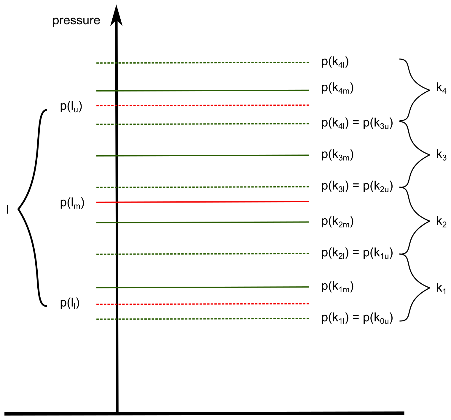
Figure B1 Schematic illustrating the vertical interpolation of ERA5 model level data to the CESM2 model levels. Red solid and dashed lines depict the midpoint and interface pressure values of one CESM2 level l, respectively, while green solid and dashed lines depict the midpoint and interface pressure values for four ERA5 levels. In the case shown here, the mass-weighted average of a variable ϕ_ERA5 at ERA5 levels k₁, k₂ and k₃ would yield the interpolated value of ϕ_ERA5 at CESM level l, ${\mathit{\varphi }}_{\text{ERA5}}^{\ast }\left(l\right)$, as for these three ERA5 levels the midpoint pressure is between the interface pressure values of the CESM2 level.

Vertical interpolation from the ERA5 model levels to the fewer CESM2 model levels is not straightforward. To explain our procedure, we introduce the notation ϕ_ERA5(k) and ϕ_CESM2(l) for vertical profiles of a variable ϕ in the two data sets, with l and k being the indices of the model levels in CESM2 and ERA5, respectively. Vertical profiles of model-level ERA5 data have been interpolated to the CESM2 model levels l in the following way (illustrated in Fig. B1): First, the pressure at each grid point and model level mid point and interface is computed in both ERA5 and CESM2. Then for any CESM2 level l all ERA5 levels k are identified whose midpoint pressure p(k_m) is between the pressure of the lower and upper interface of CESM2 level l (p(l_l) and p(l_u)). This set of levels is referred to as 𝒦. The interpolated value (^∗ denotes interpolation), ${\mathit{\varphi }}_{\text{ERA5}}^{\ast }\left(l\right)$, is then computed as mass weighted average of ϕ_ERA5(k) over all levels k∈𝒦, i.e.,

$$\begin{array}{}\text{(B1)}& {\mathit{\varphi }}_{\text{ERA5}}^{\ast }\left(l\right)={\displaystyle \frac{\mathrm{1}}{M}}\sum _{k\in \mathcal{K}}{m}_k{\mathit{\varphi }}_{\text{ERA5}}\left(k\right),\end{array}$$

whereby M is the sum of the mass in all ERA5 levels k∈𝒦 and m_k is the mass in level k.