Storylines of extreme summer temperatures in southern South America

Understanding the sources of uncertainty in future climate extremes is crucial for developing effective regional adaptation strategies. This study examines projections of summer maximum temperature (TXx) over four regions of southern South America: northern, central-eastern, central Argentina, and southern areas. We analyse simulations from 26 global climate models and apply a storyline approach to explore how different climate drivers combine to shape future changes in TXx for the late 21st century (2070–2099).

The storylines are based on changes in key physical drivers, including mid-tropospheric ridging, regional soil moisture, sea surface temperature in Niño 3.4 region and an OLR gradient index that reflects changes in atmospheric stability and the positioning of convective phenomena over the South Atlantic Ocean. A multi-linear regression framework reveals that the dominant drivers of the projected warming in TXx vary substantially across regions. In northern areas, warming is primarily influenced by remote drivers such as tropical sea surface temperatures and OLR changes in the subtropical South Atlantic. The central-eastern and central Argentina regions exhibit mixed local and remote influences, while southern areas of South America are predominantly affected by changes in local drivers (soil drying and atmospheric blocking). Together, these drivers explain up to 56 % of the inter-model spread in future projections of TXx. However, their ability to account for the uncertainty in percentile-based indices and regional heatwave characteristics is more limited, suggesting that complex heat metrics may be influenced by additional processes.

1 Introduction

Global mean surface temperature has been approximately 1.1 °C higher in 2011–2020 than in 1850–1900, with larger increases over land than over the oceans (IPCC, 2023). As a result of this warming, significant negative impacts have already been observed across various sectors of the society, including e.g. risks in water and food security (e.g., El Bilali et al., 2020; Stringer et al., 2021) or severe health effects driven by the increasing frequency of heatwaves (e.g., Amengual et al., 2014; Anderson and Bell, 2009; Ballester et al., 2023; Chesini et al., 2022). While it is unequivocal that human influence has contributed to atmospheric warming, its manifestations and impacts vary across different regions. Particularly, in South America (SA), the Sixth Assessment Report of the Intergovernmental Panel on Climate Change (IPCC) indicates that near-surface temperatures have been increasing over the past several decades, but with pronounced regional variations (IPCC, 2023). For instance, southwestern SA, particularly the Andean region, has experienced an outstanding warming (e.g., Suli et al., 2023; Vuille et al., 2015), with temperatures rising faster than the global average (IPCC, 2021). Likewise, observed trends in temperature extremes are uneven across the SA region. Northern SA reports the strongest trend in the number of days exceeding the 90th percentile during 1950–2018 (Dunn et al., 2021). However, central-southeastern SA shows contrasting results, with some studies reporting decreasing trends in warm extremes (e.g., TXx and TX90) during the austral summer (Rusticucci et al., 2017; Skansi et al., 2013; Wu and Polvani, 2017), and others indicating significant increases in the frequency of warm season heatwave days over central Argentina (Suli et al., 2023). Finally, in the southernmost part of SA, there is insufficient evidence to determine clear trends in hot extremes due to limited data availability (IPCC, 2023).

Global Climate Models (GCMs) from the Coupled Model Intercomparison Project (CMIP) have been widely used as the main tool to assess future changes in the mean and extreme values at global and continental scales (Almazroui et al., 2021b; Tebaldi et al., 2021). In SA, there are several studies on climate change projections (Almazroui et al., 2021a; Bustos Usta et al., 2022 and references therein; Feron et al., 2019; Gulizia et al., 2022; Ortega et al., 2021; Salazar et al., 2024). For instance, Almazroui et al. (2021a) evidence a substantial warming across SA, with annual mean temperature increases ranging from 2.8 to over 5.0 °C under the high-emission scenario SSP5-8.5 by the end of the century (2080–2099). The strongest warming is expected in tropical regions, particularly in the Amazon and at high altitudes such as the Andes. The latter has also been identified as a hotspot by Salazar et al. (2024), who suggest that amplified warming in the Andes may be linked to elevation-dependent responses. In southern SA, Almazroui et al. (2021a) report a weaker warming (∼ 3 °C) than in other regions, which contrasts with North America, where higher latitudes tend to exhibit stronger warming signals (Almazroui et al., 2021c). In spite of this, for 3 °C global warming levels, southeastern SA could experience a ∼ 25 % increase in warm days (TX90) compared to the 1981–2000 period (Gulizia et al., 2022).

Uncertainties in GCM projections evidenced in the multi-model ensemble cannot be directly interpreted in a probabilistic sense (Shepherd, 2019). To address structural uncertainties, Zappa and Shepherd (2017) propose a storyline-based approach, which provides physically coherent representations of plausible changes at regional scale. Each storyline is constructed by combining climate change responses based on well-known drivers that characterise the regional climate. The combination of storylines manages to capture the range of uncertainty in the future projections from multi-model ensembles (Zappa, 2019). This methodology has been applied in various regions worldwide (e.g., Bjarke et al., 2024; Gibson et al., 2024; Mindlin et al., 2020; Schmidt and Grise, 2021; Zappa and Shepherd, 2017), focusing mainly on atmospheric circulation patterns and their impacts on precipitation and droughts. Moreover, Garrido-Perez et al. (2024) extended its application to explore the uncertainty of future summer warming over Iberian Peninsula. Similarly, Mindlin et al. (2024) applied the storyline approach to examine climate impact drivers over southwestern SA, including temperature-based indices.

Various studies have demonstrated the influence of both local and remote forcings on temperature extremes in SA (Cai et al., 2020; Reboita et al., 2021; Rusticucci et al., 2003). In particular, midlatitudes of SA are strongly influenced by large-scale extratropical circulation patterns, such as waveguides, which often cause enhanced ridging activity over southern SA (O'Kane et al., 2016). Rossby wave trains also favour the strengthening of the subtropical jet over SA, increase the advection of cyclonic vorticity over southeastern SA and transport warm and moist air from the north into this region (Grimm and Ambrizzi, 2009). Likewise, Rossby wave activity is closely linked to the El Niño-Southern Oscillation (ENSO), one of the primary modes of interannual variability affecting SA (Barreiro, 2010; Cai et al., 2020; Fernandes and Grimm, 2023; Grimm and Tedeschi, 2009; Reboita et al., 2021; Rusticucci and Kousky, 2002). Most studies about ENSO impacts over SA have focused on precipitation, while its influence on summer extreme temperatures remains less explored. Although the strongest ENSO-related temperature signals in southern SA have been documented during austral winter (Cai et al., 2020; Müller et al., 2000), Rusticucci et al. (2017) reported that El Niño events are associated with a reduced diurnal temperature range north of 40° S in austral summer, suggesting a modulation of extreme temperatures during summer as well (McGregor et al., 2022).

Other remote drivers influencing the mid and low-level circulation in SA are the subtropical high-pressure systems, namely the South Atlantic High and South Pacific High. For instance, variations in the position and/or extension of the South Atlantic High can favour anomalous warming across different regions of SSA (Suli et al., 2023). Another key climatological feature of austral summer in SA is the South Atlantic Convergence Zone (SACZ) (Barros et al., 2000; Carvalho et al., 2004; Collazo et al., 2024). Particularly, an active SACZ promotes subsidence conditions over southeastern SA, favouring the development of an anticyclonic circulation there, which in turn causes warming particularly given the relatively dry conditions of the warm season (Cerne and Vera, 2011). In this context, Zilli et al. (2019) and Zilli and Carvalho (2021) identified a poleward shift of the SACZ in response to climate change, based on satellite-gauge precipitation data and CMIP5 GCM simulations. However, the disagreement among GCMs and ensemble members on simulated precipitation changes introduces substantial uncertainty in future projections of the SACZ (Carvalho and Jones, 2013).

The uncertainty associated with changes in thermodynamic components such as temperature is also modulated by non-dynamical drivers like soil-moisture coupling (Cheng et al., 2017; Hsu and Dirmeyer, 2023; Ma and Xie, 2013; Trugman et al., 2018; Vogel et al., 2017; Zhou et al., 2024). SA has been identified as a key hotspot for land–atmosphere interactions (Sörensson and Menéndez, 2011; Spennemann et al., 2018), where soil-moisture plays a crucial role in modulating surface air temperature variability (Coronato et al., 2020; Guillevic et al., 2002; Menéndez et al., 2019; Seneviratne et al., 2010). Ruscica et al. (2016) found a strong land-atmosphere coupling in central Argentina during the summer for both present and future climates. However, in northern Argentina, Uruguay, and southern Brazil, this interaction was projected to weaken in the future.

These findings underscore the complexity of assessing future projections of temperature extremes due to the multiplicity and heterogeneity of drivers across SA regions. To address this challenge, this study employs a storyline approach to dissect the climate change responses of maximum summer temperature in four regions of southern SA (SSA), aiming to better understand the drivers of structural uncertainties in GCM projections. This approach reconstructs regional projections and their associated uncertainties based on changes in different drivers of the regional climate change (e.g. Garrido-Perez et al., 2024; Mindlin et al., 2020; Zappa and Shepherd, 2017).

This paper is structured as follows. Section 2 describes the datasets and methodology used to identify key drivers for each SSA region and to construct the storylines. Section 3 presents the results, including the projected changes in the drivers, the sensitivity of the maximum summer temperature changes to these drivers, and a quantitative analysis of SSA summer temperature responses obtained from the storylines. Finally, the main findings are summarised and discussed in Sect. 4.

2 Data and methodology

2.1 Data

We used daily maximum temperature at 2 m (T2m) from the ERA5 reanalysis over SSA ([25, 60]° S and [80, 40]° W) with a regular 2.5° resolution during the austral warm seasons (October–March) of 1979–2023 (Hersbach et al., 2020). We also employed data from 26 GCMs of the Climate Model Intercomparison Project Phase 6 (CMIP6, see Table S1 in the Supplement for details). To maximise the number of models, we considered one ensemble member per GCM. Although this strategy does not remove internal variability – an issue that may require large ensembles (e.g. Deser et al., 2020, and references therein) – it does increase the sample size available for constructing the storylines (requiring three or more ensemble members per model would have reduced the ensemble to less than half its original size). Daily maximum near-surface (2 m) air temperature (TX) was used for the definition of extreme temperature indices. In addition, monthly fields of sea surface temperature (SST), soil moisture content (SM, within the top 0–10 cm of the soil), 500 hPa geopotential height (Z500) and outgoing longwave radiation (OLR) were employed for the construction of the drivers (see Sect. 2.3). GCM historical simulations (Eyring et al., 2016) over the period 1979–2014 and Shared Socioeconomic Pathway projections (SSP5-8.5, O'Neill et al., 2016) for the 2015–2099 period were obtained from the CMIP6 archive. A common 2.5° × 2.5° horizontal grid and the austral summer season (December–January–February, DJF) were considered for both reanalysis and GCM simulations. Bilinear interpolation was used for TX, SST, Z500 and OLR data, while a conservative remapping was applied to SM data to avoid spurious values (Jones, 1999).

For most of the analyses, extreme temperature conditions are diagnosed based on the summer maximum of TX (TXx). This index emphasizes the magnitude of extreme events, rather than their frequency or duration, assuming that extremes occur every summer. TXx is computed at each grid point, and at regional scales, using the regions defined in the next section. Regional TXx was calculated by first averaging TX over the region and then selecting the maximum value for each summer in order to ensure warm widespread conditions at the regional level.

2.2 Regionalisation

To identify spatially coherent regions, we followed the clustering procedure of Suli et al. (2023). Herein, the identification of homogeneous regions is based on clustering grid points with a high co-occurrence of local temperature extremes. To do so, we identified extremely warm days at each grid point as sequences of at least three consecutive days in which T2m exceeded the local daily 90th percentile of the 1981–2010 baseline period, using a 31 d moving window. Then, we applied the bottom-up Ward's hierarchical clustering method (Ward, 1963) to identify land grid points with a high co-occurrence of extremes (see Sect. 2.2 of Suli et al., 2023, for further details). As a result, five climatologically homogeneous regions were identified in SSA, which are consistent with those obtained from station-based data in Suli et al. (2023). The identified regions are depicted in Fig. 1, and named as northern SSA (NS), central-eastern SSA (CES), central Argentina and northern Argentinian Patagonia (CA), central Chile (CCH), and southern SSA (SS), including Argentinian Patagonia and southern Chile.

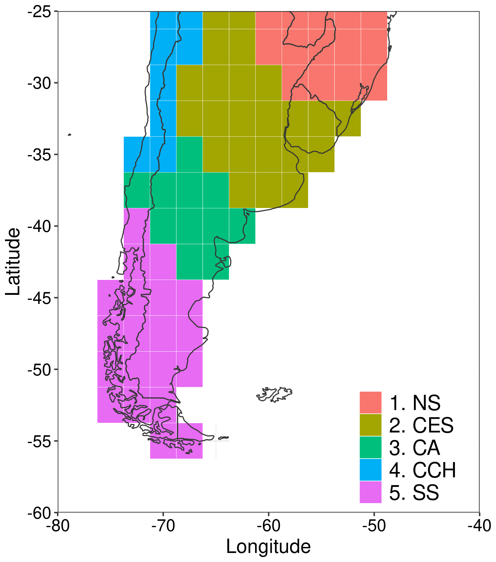
Figure 1 Regionalisation of SSA based on the co-occurrence of hot days during the warm seasons of 1979–2023. Grid points are coloured and numbered from 1 to 5, according to the region they belong: C1 – northern of SSA (NS), C2 – central-eastern of SSA (CES), C3 – central Argentina and northern Argentinian Patagonia (CA), C4 – central Chile (CCH), C5 – Argentinian Patagonia and southern Chile, southern SSA (SS).

To ensure consistency in the spatial analysis, the same SA regions of Fig. 1 were also applied to each CMIP6 GCM. However, the CCH was excluded from the analysis due to substantial temperature biases associated with unresolved topography in GCMs, which can reach magnitudes of up to ∼ 8 °C in northern Chile (Salazar et al., 2024). Note that this regionalisation aims to provide a robust characterisation of regional extremes, rather than to identify areas of homogeneous changes or high uncertainty in future projections. The latter approach would maximise the ensemble spread at regional level but would also shift the focus away from the behaviour of spatially coherent regional phenomena and their underlying drivers.

2.3 Definition of drivers

For the regional analysis, the following drivers were considered using a hybrid approach that combines linear regression analysis (Sect. 3.2) with physical reasoning (see the Introduction section, and references therein). They are grouped into local and remote drivers. Local drivers are proximate factors that directly influence regional temperature, whereas remote drivers represent large-scale influences or teleconnections affecting the region:

• Sea surface temperature in Niño 3.4 region (N3.4, remote driver): mean summer SST in the Niño 3.4 region ([5° N–5° S; 120–170° W]).

• Mid-tropospheric ridging (Z500${}_{\mathrm{HL}}^{*}$, local driver): mean summer Z500^* averaged over high latitudes (HL) of SSA [40–55° S, 60–80° W] domain (green box in Fig. 3h), where Z500^* denotes the departure of Z500 from its zonal mean. This index is used as a proxy for regional ridging activity and associated intensity of the westerlies over SSA. Positive Z500${}_{\mathrm{HL}}^{*}$ values indicate enhanced high-latitude blocking, whereas negative values reflect mid-latitude high-pressure systems (Fig. S1 in the Supplement), thus capturing the range of regional circulation patterns that favour extremely high temperatures across SSA (Suli et al., 2023).

• Regional soil moisture (SM_i, local driver): mean summer SM, averaged over the region i, with i being one of the SSA regions (SS, CA, CES or NS). We also tested the performance of drivers extending across more than one SSA region, and selected consequently a northern Argentinian subregion (SM_north, [21–31° S, 54–66° W]).

• Gradient of Outgoing Longwave Radiation (OLRg, remote driver): difference in summer mean OLR between two domains spanning 10° of latitude and 15° of longitude ([25–35° S, 10–25° W and [33–43° S, 30–45° W]], as depicted in Fig. 3b, d and f). This OLR gradient reflects regional convection patterns linked to variations in atmospheric stability. Additional analyses (Fig. S2) confirm that, on interannual scales, a strengthening of the OLR gradient is associated with an intensified or zonally elongated subtropical Atlantic anticyclone, as well as with poleward shifts in SACZ-related precipitation (Liebmann et al., 2004).

2.4 Storyline methodology

For each region, storylines describe the combined effect of the drivers' changes on summer TXx projections. Climate change responses, denoted as Δ, are computed for TXx and the drivers as the difference of the summer mean between the far future (2070–2099) and the historical period (1979–2014). The methodology used in this study follows the framework proposed by Zappa and Shepherd (2017) and is briefly described below. Firstly, we computed the climate change responses of the drivers for each region and each GCM. Secondly, the regional ΔTXx response was modelled separately for each region using an ordinary multi-linear regression (MLR, Eq. 1). In this regression, ΔTXx is the dependent variable (target), while two drivers act as independent variables (predictors):

$$\begin{array}{}\text{(1)}& {\displaystyle \frac{\mathrm{\Delta }\text{TXx}}{\text{GW}}}=a_x+b_x\cdot {\left({\displaystyle \frac{\mathrm{\Delta }{D}_{\mathrm{1}}}{\text{GW}}}\right)}_m^{\prime }+c_x\cdot {\left({\displaystyle \frac{\mathrm{\Delta }{D}_{\mathrm{2}}}{\text{GW}}}\right)}_m^{\prime }.\end{array}$$

We only considered two drivers per region in order to limit the number of storylines (given by 2ⁿ, with n being the number of drivers). Limiting the selection to two drivers also facilitates the interpretation of the storylines and helps avoid overfitting in the MLR caused by interdependencies among the predictors. In Eq. (1), ΔD₁ and ΔD₂ represent the changes in the two drivers for each model m. The symbol (^′) indicates the standardised change relative to the multi-model mean (MMM), a_x, b_x and c_x are the regression coefficients: a_x denotes the MMM intercept, representing the expected mean response when there is no deviation in the driver responses relative to the MMM; b_x and c_x quantify the sensitivity of regional ΔTXx to each driver. Both the target (ΔTXx) and the drivers (ΔD₁ and ΔD₂) were scaled by global warming (GW) defined as the corresponding change in the area-weighted global mean near-surface temperature. The MLR is based on 26 values (GCMs) and was computed separately for each region.

Once the sensitivity coefficients were obtained, regional ΔTXx can be estimated for given values of GW and drivers' responses. Combining opposite (strong or weak) responses of the two drivers for each region results in four different storylines, which reflect the corresponding effects in ΔTXx. The final ΔTXx response follows Eq. (2):

$$\begin{array}{}\text{(2)}& {\displaystyle \frac{\mathrm{\Delta }\text{TXx}}{\text{GW}}}=a_x+b_x\cdot t+c_x\cdot t.\end{array}$$

Here, t denotes the storyline index, which measures the magnitude of the driver responses (in standard deviations; SDs). In this case, the changes of the two drivers were selected to have equal standardised amplitudes, which also allows us comparing their relative effects in ΔTXx. As described by Zappa and Shepherd (2017), t was chosen to lie within the 80 % confidence region of the drivers' responses (see black stars in Fig. 4), which was obtained by fitting a bivariate normal distribution (t ∼ ±1.26 SD). Full details of the methodology can be found in Zappa and Shepherd (2017), in Appendix A of Mindlin et al. (2020) and in Garrido-Perez et al. (2024). In the construction of storylines, we assume that model biases remain constant in the future, and therefore do not substantially influence the climate change signals. Figure S3 supports this hypothesis by revealing no statistically significant relationship between model biases in TXx and their projected changes, ΔTXx. Furthermore, recent studies indicate that CMIP6 models reproduce the climatology and seasonal variability of the aforementioned drivers reasonably well over SSA when compared with ERA5, including challenging variables like SM (Qiao et al., 2022).

3 Results

3.1 Variability of projected changes

Figure 2 shows the MMM summer projections of TXx and the drivers used in this study for 2070–2099 (with respect to 1979–2014). Consistent with Almazroui et al. (2021a), tropical regions in northern SA exhibit a strong significant warming by the end of the century, exceeding 5 °C. In SSA, the largest TXx increases are projected along the Andes Mountains (Fig. 2a), aligning with Salazar et al. (2024), who reported a warming of up to 6 °C in northern Chile. In contrast, central SSA regions display a more homogeneous and less pronounced warming of approximately 4 °C (Lagos-Zúñiga et al., 2024).

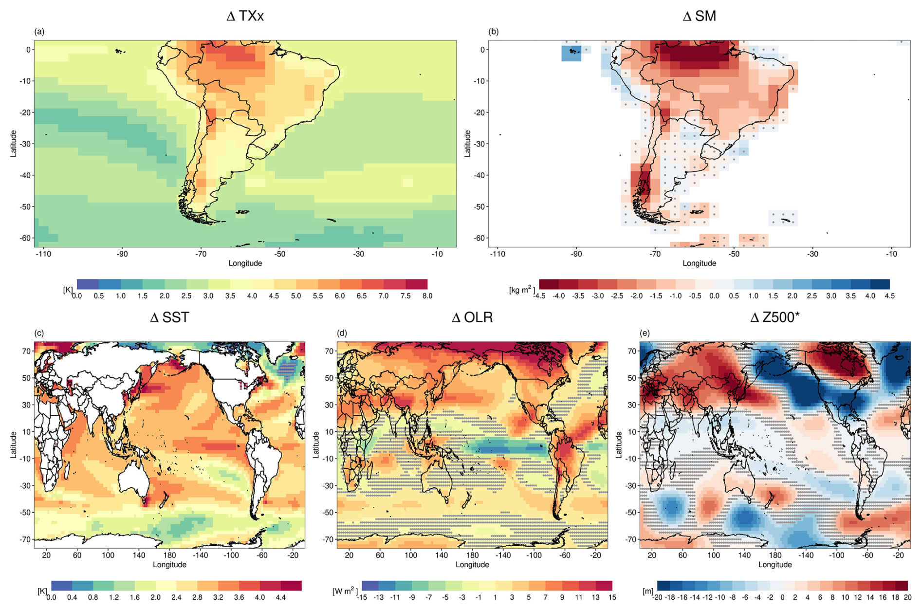
Figure 2 Multi-model mean (MMM) summer (DJF) changes in (a) Maximum Temperature (TXx, K), (b) Soil Moisture (SM, kg m⁻²), (c) Sea Surface Temperature (SST, K), (d) Outgoing Longwave Radiation (OLR, W m⁻²) and (e) Geopotential Height at 500 hPa with the zonal mean removed (Z500^*, m). Changes are computed as the difference between the periods 2070–2099 and 1979–2014. Grey dots indicate areas where changes are not statistically significant at the 95 % confidence level, based on a two-tailed t test.

Concerning the projected changes in the climate drivers, SM is expected to decrease significantly over northern SA, especially in the Amazon and along the Andes Mountains (see Fig. 2b), consistent with Cheng et al. (2017). In contrast, future SM projections for central-eastern SSA remain uncertain. In this region, CMIP5 GCMs projected positive SM changes for 2061–2080 compared to 2006–2025 under a high emission scenario (Cheng et al., 2017). However, more recent CMIP6 projections under SSP5-8.5 show no consistent changes in regional SM (Cook et al., 2020). As this region is characterised by strong soil-atmosphere coupling, the uncertainties in SM projections are expected to propagate to summer temperature changes.

Regarding SSTs, the central-eastern Pacific is projected to warm by up to 4 °C above historical values by the end of the century (Fig. 2c). This warming enhances convection over the region as it can be seen by negative changes in OLR (Fig. 2d). Pronounced warming is also observed in the western Pacific Ocean near southeastern Australia (Fig. 2c), as noted by other authors (Lenton et al., 2015; Oliver et al., 2014). Although the direct impact of the western Pacific Ocean warming on SA remains uncertain, Sun et al. (2023) suggested that air-sea coupling in the tropical Pacific greatly amplifies the atmospheric response of the South Pacific to ENSO. Indeed, ΔZ500^* exhibits alternating anomalies over the Pacific that resemble a Rossby wave pattern extending from southern Australia (Fig. 2e), which has been associated with heatwaves in the subtropical SA (Cerne and Vera, 2011; Shimizu and de Cavalcanti, 2011). In addition, enhanced anticyclonic conditions are projected in southern SA, particularly at high latitudes, which may be linked to an increasing zonal asymmetry of the Southern Annular Mode during DJF (Campitelli et al., 2022).

3.2 Selection of drivers

To identify remote and local drivers of ΔTXx, we examined the regression patterns of several variables and constructed indices displaying a strong and physically consistent relationship with regional TXx. Figure 3 illustrates the linear regression patterns of these field responses onto regional ΔTXx. Figure 3a shows significant positive SST regression coefficients over the tropical Pacific (yellow box) suggesting that enhanced El Niño events contribute to increase ΔTXx in NS. Although El Niño is currently associated with cooler TXx conditions in this region compared to La Niña (Arblaster and Alexander, 2012), future projections suggest a weakening of the ENSO-related temperature signal over SSA (McGregor et al., 2022). Consequently, El Niño events may exert a reduced cooling effect in the future, resulting in higher TXx values relative to the present, and thus contributing to a positive ΔTXx response. In addition, changes in the OLR gradient (ΔOLRg) act as an important remote driver of NS ΔTXx (Fig. 3b). In particular, enhanced mid-latitude convection (negative ΔOLR in the poleward box) and/or suppressed subtropical convection (positive ΔOLR in the equatorward box) is associated with amplified warming over this region.

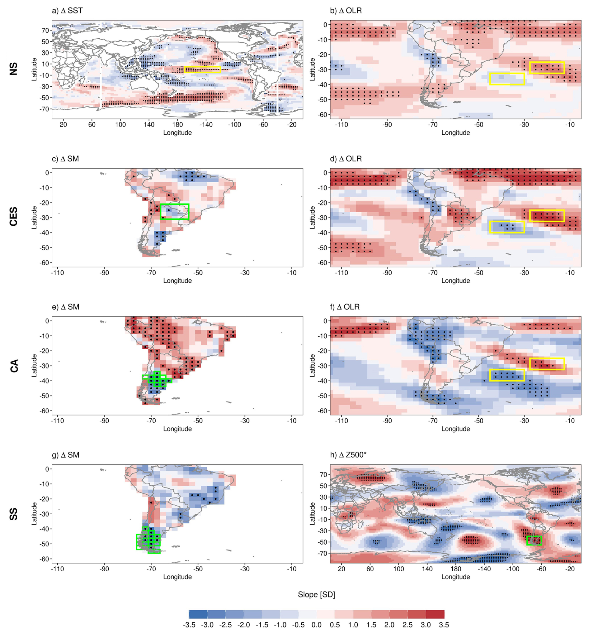
Figure 3 Regression-based summer changes in several fields (expressed in SD with respect to the MMM) corresponding to a 1 K K⁻¹ regional scaled warming (ΔTxx/GW, 2070–2099 minus 1979–2014) for: NS: (a) ΔSST and (b) ΔOLR; CES: (c) ΔSM and (d) ΔOLR; CA: (e) ΔSM and (f) ΔOLR; SS: (g) ΔSM and (h) ΔZ500^*. Boxes indicate the regions used to construct regional driver indices for the MLR analysis. Local drivers are denoted in green and remote drivers in yellow. Stippling denotes statistically significant regression coefficients at p < 0.1, after a two-tailed t test.

For the other regions, ΔOLRg also acts as a remote driver of ΔTXx in CES, where regional warming concurs with an anomalous configuration of the subtropical Atlantic anticyclone, or with modified SACZ-related convection (Suli et al., 2023). Furthermore, projected drying over northern Argentina and Paraguay (green box in Fig. 3c) is consistent with a CES warming response, although significance is limited to few points, possibly reflecting a weakened soil–atmosphere coupling under future climate conditions (Ruscica et al., 2016). Regarding CA (Fig. 3e–f), the results show that GCM projections with larger decreases in SM_CA or an enhanced OLRg display more pronounced TXx warming. Finally, the largest warming in SS (Fig. 3g–h) is associated with reduced SM_SS and an anomalously high Z500^* over SSA. The influence of SM_SS is consistent by Collazo et al. (2024), who found that southern SA exhibits strong soil-atmosphere coupling during the warm season, despite its aridity. Likewise, the Z500${}_{\mathrm{HL}}^{*}$ driver captures high-latitude blocking, which has been linked to SS heat extremes (Suli et al., 2023). Previous studies also indicate that anticyclonic anomalies over southern SA can trigger heatwaves in this region (Cerne and Vera, 2011; Collazo et al., 2024; Jacques-Coper et al., 2016).

In the following, different MLR models (see Eq. 1), based on the climate change responses of TXx and the regional drivers described in Sect. 2.3 were performed for each SSA region. Sensitivity tests were also conducted to assess whether lagged relationships between the changes in the drivers and regional TXx could improve the model performance. However, no significant improvement was found when introducing temporal lags. Therefore, we focused on simultaneous summer responses in both drivers and TXx. We also verified that the selected drivers were not significantly correlated with each other (i.e. Pearson correlation coefficients with p values > 0.1) to avoid redundant information that would add unnecessary complexity to the model and the interpretation of the drivers.

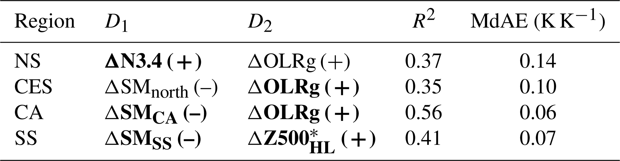
The final combination of drivers is outlined in Table 1, along with the sign of their regression coefficients ($+/-$) and the corresponding explained variance (R²). The selected drivers vary across SSA regions. In NS, the warming response in TXx is substantially affected by changes in remote drivers (ΔN3.4 and ΔOLRg), while in SS only local drivers are identified (ΔSM_SS and ΔZ500${}_{\mathrm{HL}}^{*}$). In contrast, both local and remote drivers (ΔSM_i and ΔOLRg) affect the warming of extremes in CES and CA. For all regions, the uncertainty in the drivers' changes is significantly correlated with that in TXx, except for CES, where ΔSM_north does not show a significant response in ΔTXx. Although this region exhibits a strong soil-atmosphere coupling on interannual timescales (Jung et al., 2010; Ruscica et al., 2015; Sörensson and Menéndez, 2011), the lack of significance indicates that SM_north cannot explain the spread of TXx projections in this area. For all regions, R² exceeds 35 %, with the highest values observed in SS (R² ∼ 41 %) and CA (R² ∼ 56 %).

Table 1 Drivers used to perform the MLR (Eq. 1) for each SSA region. The symbol in parentheses (“+” or “–”) specifies the sign of the regression coefficient and bold values denote statistically significant coefficients (p < 0.1). The last columns indicate the coefficient of determination (R²) and the median absolute error (MdAE, in K K⁻¹) obtained from the MLR.

3.3 Storylines analysis

Four storylines (herein labelled as ST#, with # ranging from 1 to 4) of future summer TXx changes were constructed based on the combination of the two most influential drivers of ΔTXx in each region described in Sect. 3.2. Figure 4 depicts the scatterplots of the two drivers' responses within the CMIP6 ensemble, along with the standardised change amplitudes selected to construct each storyline (represented by black stars), following the regression framework described in Sect. 2.4. GCMs that displayed a systematic outlier behaviour across all regions were excluded from the analysis. The results show considerable uncertainty in driver responses. Some drivers show consistent changes in sign but have uncertain magnitudes (e.g., N3.4 and the SM_SS index, see Fig. 4a and d), while for others, both the sign and magnitude of the change are uncertain (e.g., SM_CA or OLRg, see Fig. 4c). For all drivers, the spread of responses across the multi-model ensemble is clearly distinguishable from the internal variability. To illustrate this, we compared the magnitude of the projected changes in the selected drivers with an estimate of the internal variability based on the interannual standard deviation of the detrended series, following the approach in Mindlin et al. (2020, their Appendix B). The results (Table S2) show that the variability within individual models is significantly lower than across models (inter-model variability), indicating that the spread in driver projections is primarily driven by model uncertainty rather than by internal variability.

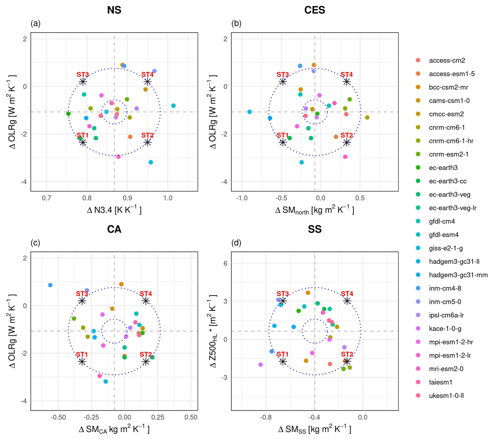
Figure 4 Drivers' responses scaled by global warming (GW) for each GCM (colour circles) across SSA regions: (a) NS, (b) CES, (c) CA, and (d) SS. Black stars indicate the four storylines of ΔTXx derived from extreme responses of the two most influential drivers (see Eq. 2). Dashed black ellipses indicate the 80 % confidence region, obtained by fitting a bivariate normal distribution to the GCM responses. Each quadrant displays the combination of the two drivers associated with each storyline.

Each storyline characterises the summer ΔTXx as the combined response in b_x and c_x (see Eq. 2), yielding distinct patterns of warming depending on how the two drivers change. For instance, ST1 for the NS region (Fig. 4a and first row of Table 2) is characterised by lower-than-MMM changes in both N3.4 and OLRg, while ST4 represents the opposite pattern. Similarly, ST2 and ST3 correspond to opposing changes in these two drivers. The specific combination of drivers for each ST and region, as obtained from Fig. 4, is summarised in Table 2.

Table 2 Combination of drivers selected to create the corresponding storylines (ST1 to ST4, columns) of ΔTXx for each region (rows).

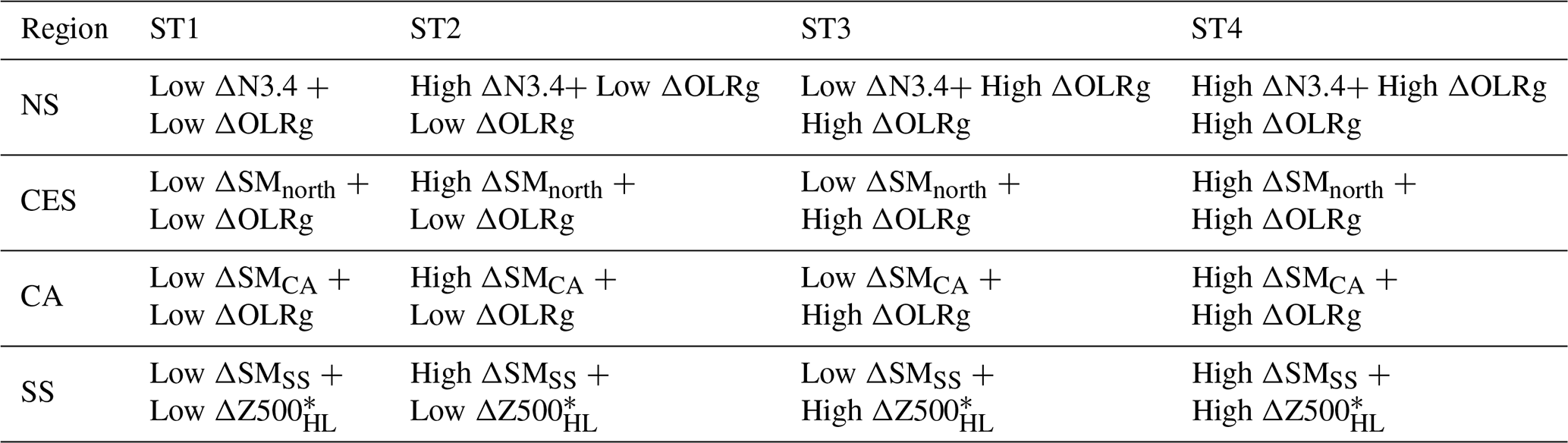
Figure 5 illustrates the scaled summer ΔTXx for each GCM (coloured circles), including the MMM (black diamond) and its 1 SD range (grey shading), as well as the reconstructed storylines of ΔTXx (coloured squares) based on the combination of drivers' responses. This figure also reveals which combination of drivers leads to the largest and smallest warming in each region, i.e. the worst-case and best-case scenarios, respectively. Overall, TXx warming appears unavoidable, as even the best-case scenario shows an increase of ∼ 0.9 K K⁻¹ across all regions. Moreover, the TXx warming response in the worst-case storyline is 29 % to 54 % higher than in the best-case scenario. To measure the robustness of the storylines, we compared the difference between opposite storylines (Fig. 5) with the median absolute error (MdAE) of the MLR (Table 1) for each SSA region, similar to Mindlin et al. (2020). In most regions (NS, CA and SS), the MdAE represents less than ∼ 25 % of the storyline responses. In CES, the MdAE represents a higher fraction of the differences between storylines (∼ 35 %), which may be due to the lack of significance of one of the drivers. Overall, these results confirm that the regression-based framework provides a meaningful representation of the TXx responses across SSA. Indeed, the inter-storyline variability reasonably encompasses the range of uncertainties in ΔTXx projections, represented by the grey-shaded areas in Fig. 5a–d. In the remainder, the two remaining storylines will not be discussed, as they exhibit an intermediate result.

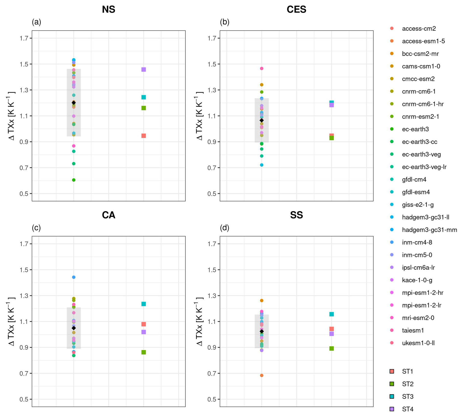
Figure 5 Summer (DJF) TXx responses (2070–2099 minus 1979–2014) per degree of GW (K K⁻¹) for each GCM (coloured circles) and for each SSA region: (a) NS, (b) CES, (c) CA, and (d) SS. The black diamond denotes the MMM and the grey-shaded area indicates its 1 SD. The four storylines are depicted with filled colour squares.

In NS, the largest warming in TXx (ST4, purple square; Fig. 5a) results from the combination of a warming in the tropical Pacific and a strengthening of the OLRg relative to the MMM changes. This storyline determines a 54 % greater increase in ΔTXx compared to the opposite combination of drivers' responses. Differenly, Mindlin et al. (2024) found a larger increase in October–April mean TX over southwestern SA under a low Pacific warming storyline (i.e. a relative cooling of both eastern and central El Niño), whereas a high Pacific warming produced the opposite response. The discrepancies with our findings may stem from differences in the selected drivers, target variables, seasonal definitions, and/or regional domains. CES and CA storylines are constructed using similar drivers (as seen in Table 1). However, the response in ΔTXx differs between the two regions. For CES, ΔOLRg is the only driver with significant influence on ΔTXx (Table 1; Fig. 5b). This is reflected in the separation between the storylines. ST1 and ST2 are associated with a weakening of the OLRg, whereas ST3 and ST4 correspond to a weak intensification of the OLRg (Fig. 4b and Table 2), with the latter yielding an additional ∼ 29 % increase in ΔTXx. Comparatively, the difference in ΔTXx between ST1 and ST2, as well as between ST3 and ST4, is negligible. This pattern highlights that the spread of ΔTXx projections over CES is primarily driven by OLRg variations, likely linked to changes in the subtropical Atlantic anticyclone or in SACZ-related precipitation, while ΔSM_north does not play a significant role. In contrast, in CA, the combination of strong drying and an intensification of the OLRg leads to a ΔTXx warming ∼ 44 % higher than that associated with the opposite storyline (Fig. 5c). Finally, the storyline characterised by the largest warming in SS ΔTXx (ST3, blue square; Fig. 5d) is determined by the combination of enhanced drying and anticyclonic activity relative to the MMM, with an additional 30 % increase in ΔTXx warming compared to the best-case storyline (ST2, green square).

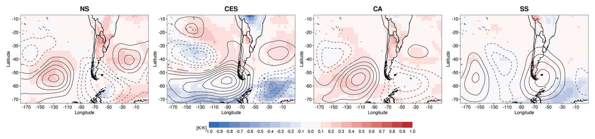
Figure 6 Differences between the composites of projected changes in TXx (shading, K K⁻¹) and Z500^* (in contours, m K⁻¹) for the GCMs with the strongest (worst-case storyline) and weakest (best-case storyline) warming in regional TXx: (a) NS, (b) CES, (c) CA, and (d) SS. Contours are shown every 1 m K⁻¹, with solid (dashed) black lines representing positive (negative) ΔZ500^*. Values are expressed per degree of GW.

For better interpretation of the differences in the storylines of ΔTXx, Fig. 6 shows the composite difference of the spatial patterns of ΔTXx (shading) and ΔZ500^* (contours) between the GCMs following the worst- and best-case storyline of regional ΔTXx (i.e. GCMs falling within the 80 % confidence interval of the corresponding quadrant in Fig. 4). Enhanced warming under the worst-case outcome is evident across all regions, particularly in NS. In contrast, in CES, the ΔTXx differences between extremal storylines are small, consistent with the poorer MLR performance and the weak influence of one of its drivers. The worst-case scenarios of each region are also accompanied by distinctive circulation anomalies, featuring Rossby wave trains with different pathways and latitudes depending on the region, which are consistent with the enhanced regional ΔTXx responses. Likewise, in NS, CES, and to a lesser extent CA, the drivers associated with the largest warming in ΔTXx lead to anticyclonic anomalies over the South Atlantic Ocean. This is consistent with Suli et al. (2023), who found that heatwaves in these regions are triggered by shifts/intensification of the subtropical semi-permanent high-pressure systems. The influence of the subtropical anticyclone is missing in the worst-case storyline of SS, where extremely warm days are related to co-located anticyclonic anomalies (blocking) and jet meandering.

Overall, these findings underscore the importance of identifying region-specific drivers and exploring physically plausible scenarios beyond the MMM. For all regions, we find that changes in both thermodynamic (regional SM, N3.4) and dynamic (Z500${}_{\mathrm{HL}}^{*}$, OLRg) drivers contribute to the spread of future projections in regional ΔTXx, stressing the importance of understanding dynamical aspects of climate change in the region.

4 Conclusions and discussion

In this study we assessed the sources of uncertainty in maximum summer temperature (TXx) projections over Southern South America (SSA) using historical and future simulations of 26 global climate models (GCMs) from the Coupled Intercomparison Project Phase 6 (CMIP6). To do so, we applied a storyline approach to TXx changes (ΔTXx) in four subregions of SSA: northern SSA (NS), central-eastern SSA (CES), central Argentina (CA) and southern SSA (SS). Storylines were created for each region based on the climate change responses in key drivers of ΔTXx, including mid-tropospheric ridging (Z500${}_{\mathrm{HL}}^{*}$), regional soil moisture (SM), sea surface temperature in the Niño 3.4 region (N3.4), and the gradient of outgoing longwave radiation over the South Atlantic Ocean (OLRg). The main results can be summarised as follows:

• Future changes in the drivers of SSA temperature extremes: the multi-model mean (MMM) changes at the end of the century (2070–2099) reveal a strong soil drying in central northern SA and along the Andes mountains, while SM changes over central SSA remain uncertain. The central-eastern Pacific is projected to warm by up to 4 °C above historical values, enhancing convection over the region. Moreover, changes in Z500^* feature a Rossby wave pattern with alternating high-low-pressure anomalies over the high latitudes of SA and the mid-latitudes of the adjacent oceans. However, these elements can have competing effects on regional ΔTXx, and their responses to climate change are affected by substantial uncertainty, which propagates to that in the future projections of regional ΔTXx.

• Relevant regional drivers of SSA temperature extremes: several physically coherent drivers were considered, and the most relevant combinations were identified for each SSA subregion. After that, a multi-linear regression (MLR) was applied to study the regional TXx responses to the drivers' changes previously found. Different drivers influence ΔTXx depending on the region: in NS, ΔTXx was primarily linked to remote influences (ΔN3.4 and ΔOLRg). For CES and CA, both remote and local factors contributed, namely ΔSM and ΔOLRg. In contrast, in SS, the projected warming was mainly explained by proximate factors, particularly regional soil drying and ridging. The MLR accounted for 35 % to 56 % of regional ΔTXx variance, with significant predictors in most regions, except for SM in CES, where its influence was negligible.

• Storylines of changes in regional temperature extremes: The magnitude of the projected summer warming in regional ΔTXx depends on specific combinations of its climate drivers, which vary from region to region. The storylines capture the inter-model variability of ΔTXx and help explain the physical mechanisms behind their uncertainties. Differences between the best- and worst-case storyline ranged from 29 % to 54 %, with NS region showing the greatest sensitivity to drivers' combinations. In this region, the highest warming in ΔTXx resulted from enhanced central-eastern Pacific warming with respect to the MMM, which is associated with El Niño events, and OLRg intensification, leading to a ∼0.5 K K⁻¹ (over 50 %) increase compared to the opposite combination of drivers' responses. In SS, the strongest warming in ΔTXx was linked to enhanced soil drying and anticyclonic activity, while soil drying and OLRg intensification resulted in the worst-case storyline for CA. Finally, in CES, the warming in ΔTXx is primarily driven by the strengthening of the OLRg, with soil moisture playing a negligible role.

Therefore, future projections of TXx in SSA show spatial variations, and their uncertainties are governed by different drivers, which often encompass local and remote factors representing thermodynamic and dynamical aspects of climate change. Given this, it is also relevant to assess whether such drivers depend on the specific aspect of the extreme event that is being scrutinized (i.e. the extreme index). Additional analyses reveal that regional ΔTXx drivers show varying skill to explain uncertainties in future projections of more complex metrics, such as the percentage of summer days exceeding the 90th percentile (TX90). The regional responses of TX90 to the aforementioned drivers are generally weaker than those in TXx, being mostly non-significant (see Table S3), with a reduction in the explained variance of 0.13–0.35 across most regions (not shown). Statistically significant responses were only found in CA and SS, where enhanced ΔTX90 was associated with strong regional soil drying and intensified anticyclonic activity, respectively. However, the remaining drivers of ΔTXx in these regions did not show a significant response in TX90, and none of the ΔTXx drivers in NS and CES explained a significant fraction of ΔTX90 variance. Similar results are found for heatwave attributes (i.e. duration, areal extent, and intensity; Table S3) derived from a spatio-temporal tracking algorithm (Sánchez-Benítez et al., 2020) applied to characterise heatwaves in Argentina (Collazo et al., 2024).

These differences suggest that the drivers of absolute summer temperature differ from those based on relative thresholds like TX90, arguably reflecting different sensitivities to changes in the mean and variability of extremes (Barriopedro et al., 2023, and references therein). Garrido-Perez et al. (2024) found similar results when analysing extreme temperature responses in the Iberian Peninsula from a variety of indices. Regardless of the causes, the observed differences indicate that the drivers and associated storylines of extremes should not be generalised to all indices and attributes. The use of emerging tools, including artificial intelligence (e.g., Pérez-Aracil et al., 2025) may help uncover additional drivers on extended spatio-temporal scales, and the differences across extreme indices.