Multi-model high-resolution analysis of Tropical-Like Cyclone Daniel with WRF and ICON: peculiarities and sensitivity to convection schemes

Medicane Daniel (September 2023) featured a multi-stage transition from a baroclinic disturbance to a compact tropical-like vortex, culminating in a rapid barotropic alignment on 9 September, challenging short-range prediction. This study delivers a side-by-side, high-resolution (∼ 2 km) assessment of Daniel using two state of the art weather forecasting models, WRF and ICON, configured to be as comparable as possible in terms of domain, forcing and vertical discretizations. Seven numerical simulations are compared assessing also sensitivity to the convection scheme: fully explicit, deep-cumulus parameterized and independent shallow-convection options (plus ICON's grayzone setting). Analysis methods include an objective cyclone tracker that combines mean sea-level pressure and lower tropospheric geopotential structure, intensity metrics (central pressure and 10 m wind) along the track, precipitation anomalies regridded against IMERG observations (Integrated Multi-satellitE Retrievals for GPM). Tropical characteristics are examined with Hart's Cyclone Phase Space and Temporal Annular Symmetric Mean (TASM) of equivalent potential temperature and wind to distill three-dimensional, time-mean storm structure during the peak warm-core phase.

Both models reproduce Daniel's life cycle and produce realistic tracks. Intensity of the cyclone sharply varies from simulation to simulation, with different behavior of each model at changes in convection scheme.

The study emphasizes the different responses of the two models both in reproducing such an extreme meteorological phenomenon and in the variation of the convection scheme. Practical suggestions are established depending on the case study and the resolution used.

1 Introduction

The Mediterranean Sea frequently experiences cyclones that either originate within the basin or migrate from surrounding regions. Some systems undergo rapid intensification and may even develop tropical-like characteristics, producing strong winds, heavy rainfall and coastal flooding, which can lead to significant regional impacts (Carniel et al., 2024).

Formally

a “MEDiterranean hurriCANE” (medicane) is a mesoscale cyclone that develops over the Mediterranean Sea and displays tropical-like cyclone characteristics: a warm core extending into the upper troposphere, an eye-like feature in its center with spiral cloud bands around, an almost windless center surrounded by nearly-symmetric sea-surface wind circulation with maximum wind speed within a few tens of km from the center (Miglietta et al., 2025).

Hence, the terms medicanes and Mediterranean Tropical-Like Cyclones (TLCs) should be considered equivalent.

Although formation mechanisms are partially understood (Miglietta, 2019), the catastrophic effects resulting from strong winds and heavy rainfall underscore the importance of correctly forecasting these phenomena, for early warning, prevention, and adaptation (Khodayar et al., 2025).

Several studies have shown that the predictability of intense cyclones in the Mediterranean area is very low (Doiteau et al., 2024). Furthermore, there is no consensus on which model performs best in simulating TLCs, as results can vary depending on the specific event, model configuration and evaluation metrics used. Many studies have already performed sensitivity analysis on the microphysics parameterizations, the Planetary Boundary Layer schemes and on the initialization time or dataset (Ricchi et al., 2017; Pytharoulis et al., 2018; Ricchi et al., 2019), showing extreme variability of the results, especially on the track of the medicanes. Among the many options available, the cumulus parameterization can play a key role, not only in terms of the path and intensity of the cyclone (Biswas et al., 2014; Miglietta et al., 2015; Saraceni et al., 2023), but also for the amount and location of the precipitation.

From this perspective, we propose to evaluate the performance of two consolidated Numerical Weather Prediction (NWP) models: WRF (Weather Research and Forecasting) and ICON (ICOsahedral Nonhydrostatic).

WRF is a mesoscale model developed by the National Center for Atmospheric Research (NCAR), the National Oceanic and Atmospheric Administration (NOAA), and the Air Force Weather Agency (AFWA). It is widely used thanks to its flexibility, scalability and a comprehensive set of physical parameterizations (Skamarock et al., 2021).

ICON is a model developed by the Deutscher Wetterdienst (DWD) and the Max Planck Institute for Meteorology (MPI-M). It employs a unique grid structure based on an icosahedral mesh, which allows efficient parallelization and improved representation of atmospheric processes at various scales from global to limited area (Zängl et al., 2015).

The choice of these two models is motivated by their widespread use in both research and operational forecasting. Specifically, a horizontal grid spacing of ≈ 2 km is representative of the current convection-permitting operational standard adopted by major national meteorological services and regional research institutes like ICON-D2 at ∼ 2.2 km by DWD (2026), ICON-2I at ∼ 2.2 km by ItaliaMeteo (2026), ICON-CH2 at ∼ 2.2 km by MeteoSwiss (2026), WRF at ∼ 4–1 km by MeteoGalicia (2026), WRF at ∼ 3–1 km by CETEMPS (2026), WRF at ∼ 2 km by CMCC (2026).

The selected case study focuses on Medicane Daniel developed in September 2023. The event was marked by exceptionally low forecast predictability (Flaounas et al., 2025) and led to widespread and severe socio-economic consequences, causing extensive damage and loss in large parts of Greece and Libya (Diakakis et al., 2025).

One of the objectives of this study is to perform a systematic comparison between the WRF and ICON models in their ability to simulate the track, intensity evolution, precipitation structure and tropical-like characteristics of TLC Daniel. Particular attention is paid to evaluate how consistently each model reproduces the observed dynamical and thermodynamical features associated with the system, including its warm-core structure, the mesoscale organization and the moisture distribution. Furthermore, the study aims to quantify the sensitivity of both modeling frameworks to different representations of convective processes, specifically contrasting simulations employing explicit convection, partially parameterized schemes and fully parameterized approaches. By examining these configurations, we seek to identify the extent to which convective treatment influences the storm development, precipitation and track predictability. Ultimately, providing insights into model-dependent uncertainties relevant for the simulation of Mediterranean tropical-like cyclones.

The study is structured as follows: Sect. 2 provides insights into the selected case study. Section 3 describes the data and methods used, including model configurations, observational data and evaluation metrics. Section 4 presents the results of the simulations, focusing on track, intensity, precipitation and tropical characteristics. Section 5 discusses the findings, highlights the strengths and weaknesses of each model and provides conclusions and recommendations for future research.

2 Case study: Tropical-Like Cyclone Daniel

The TLC Daniel developed on 4 September 2023 and lasted until 12 September 2023 and still represents one of the most destructive Mediterranean cyclones on record. Its life-cycle can be subdivided into five main phases: genesis, extratropical development, transition, tropical-like maturity and dissipation (Fig. 1; data from ERA5; Hersbach et al., 2023b). The system caused catastrophic flooding in Greece during its initial stages and later in Libya at peak intensity during the tropical-like phase, resulting in severe socioeconomic impacts and loss of life (Hewson et al., 2024).

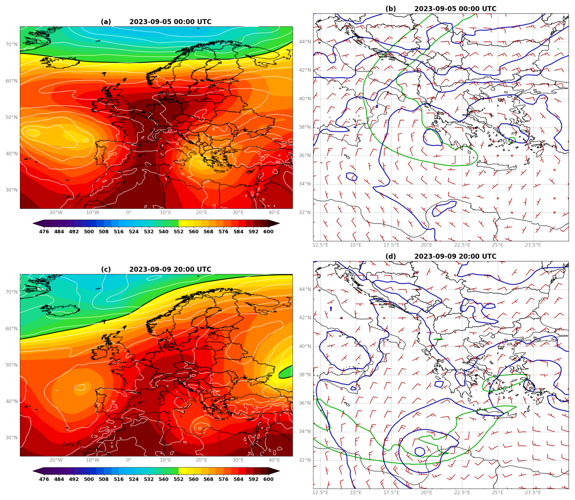
Figure 1 (a) Synoptic scale structure of TLC Daniel at: genesis stage 5 September 2023 00:00 UTC for 500 hPa Geopotential (gpdm, filled contours) and for MSLP (hPa, white contours); (b) 300 hPa 2 PVU (green contour), MSLP (blue contour) and 850 hPa wind (red barbs). At the tropical stage 9 September 2023 20:00 UTC: (c) the same as panel (a) and (d) the same as panel (b). Data from ERA5.

Daniel originated on 4 September 2023 over the Aegean Sea as an extratropical disturbance embedded within a pronounced omega blocking pattern over Europe (Fig. 1a). The anticyclonic Rossby wave breaking resulted in the intrusion of an upper-level PV streamer into the central Mediterranean basin, triggering cyclogenesis near the coast of Greece (Fig. 1b).

On 5–6 September, the low-pressure system, centered in southwestern Greece, induced persistent easterly to northeasterly flow over mainland Greece. This circulation pattern facilitated strong low-level moisture transport from the Aegean and Black Seas. As a result, widespread thunderstorms developed, with cloud tops exceeding 13 km, producing extreme precipitation and severe flooding throughout central and eastern Greece, as well as parts of Bulgaria and Turkey. Surface stations recorded more than 750 mm of daily rainfall and up to 1235 mm in 4 d in the eastern parts of the Thessaly region (Lagouvardos et al., 2017).

By 7–8 September, during a slow southward drift toward the central Mediterranean, the cyclone moved over progressively warmer waters, diabatic processes intensified, marking the onset of a subtropical transition. TheSea Surface Temperature (SST) in the south of Greece and near the Libyan coast approached 28 °C, providing an anomalously large energy reservoir for the system (Argüeso et al., 2024).

On 9 September, Daniel underwent a marked structural transformation. The surface pressure continued to decrease, the winds intensified and the vortex barotropically aligned (Fig. 1c, d). These characteristics are consistent with a tropical-like cyclone, or medicane.

Daniel made landfall near Benghazi at approximately 01:00 UTC on 10 September 2023. At peak intensity, the cyclone produced strong winds up to 70–80 km h⁻¹ and exceptional accumulated rainfall in northeastern Libya. Observed precipitation ranged from 150 to 240 mm in many locations: Al-Bayda recorded a daily accumulation of 414.1 mm, establishing a new national rainfall record. The extremely large runoff led to the collapse of two ageing dams near Derna, resulting in catastrophic flooding that destroyed entire neighbourhoods and caused thousands of fatalities (IOM, 2023; WMO, 2023).

After the landfall, Daniel began to weaken as it moved eastward on land, reducing its marine energy source. By 11 September, the cyclonic circulation persisted at low levels in the east of Libya and the north of Egypt. During this phase, counter-clockwise flow around the system facilitated the uploading and advection of mineral dust from the Western Desert of Egypt, generating a significant dust outbreak observed in satellite imagery. Dust transport continued until 12 September as the system further dissipated.

In summary, the impact of Daniel can be divided into two distinct stages: the cyclogenesis phase that impacts Greece and the mature tropical-like phase that impacts Libya. Forecast skill differed markedly between these stages. Medium-range ensemble predictions exhibited limited skill in forecasting cyclogenesis beyond lead times of 4–5 d, mainly due to difficulties in accurately representing the PV streamer intrusion. In contrast, once the cyclone had formed, the ensemble forecasts showed greater confidence in predicting its track and eventual landfall in Libya (Flaounas et al., 2025).

3 Data and Methods

3.1 Models configuration

The NWP models used for the simulations are WRF v4.6.0 and ICON v2.6.6 in Limited Area Model (LAM) configuration. In order to ease the comparison, the differences between the two models are reduced by setting the running configurations as close as possible.

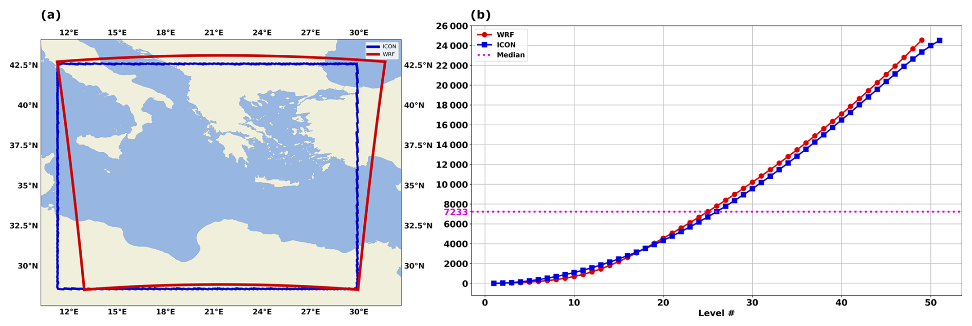
Figure 2 (a) The domains outline for WRF (red) and ICON (blue) models. (b) The vertical levels distribution for WRF (red) and ICON (blue) models; in purple dashed line the height of the median of the levels distribution.

Only one domain is used for both models, the WRF one was built first. The Lambertian conformal conical projection facilitates the creation of a domain whose contour does not intersect high mountain ranges along the edges or especially at the corners, avoiding possible disturbances that could result from the orography. Then the ICON domain in a rectangular plan was then adapted as best as possible to cover the same area as WRF (Fig. 2a). The resulting domains extend approximately in the range [11.3° E, 31.6° E, 28.5° N, 43.1° N].

The spatial resolution was set to 2 km, because operationally this is approximately the resolution used by both models.

Consequently, in compliance with the Courant-Friedrichs-Lewy condition, the timestep was set to 6 s for both models. The runs are initialized at 00:00 UTC on 4 September 2023, and end at 00:00 UTC on 12 September 2023, with output every hour. The analyses produced with the Integrated Forecasting System (IFS) by the European Centre for Medium-Range Weather Forecasts (ECMWF) (ECMWF, 2023) are used as Initial (IC) and Lateral Boundary Conditions(LBC), with Boundary Conditions every 6 h with a nominal spatial resolution of 0.8° × 0.8°. In order to validate the long simulation carried out for Daniel, three separate simulations were performed, initialized according to the three major phases described, covering the entire event with approximately 72 h each. But the outcome is a deterioration in the reproduction of the track and tropical characteristics, probably due to the spin-up (cold start) of each re-initialised run; a dedicated analysis is left for future work.

The choice of a single domain with a grid spacing of ≈ 2 km was carefully evaluated. Given the ≈ 9 km LBCs, a direct downscaling to 1 km would introduce severe boundary reflections, while intermediate nests introduce cascading interpolation artifacts and complex dynamical noise (Miglietta et al., 2023). Furthermore, differing structural nesting ratio constraints between the models (e.g., odd integers in WRF versus powers of 2 in ICON) would produce unmatched parent domains, compromising a clean model intercomparison. Physically, ≈ 2 km represents an optimal intermediate “sweet spot” between coarse parameterizations and fully resolved ones (Brumer et al., 2026). The grid-spacing regime, ≈ 2 km is classified as convection-permitting rather than a classic deep-convection gray zone (typically 3–10 km); nevertheless, it sits squarely in the physical gray zone for shallow convection, boundary-layer turbulence, and individual updraft dynamics, which remain only partially resolved.

Vertical discretization is one of the important characteristics of the model to be taken into account when configuring it. In fact, a good representation of the lower layers is necessary where the cyclone interacts with the sea surface, as well as a good representation of the upper layers, where the jet stream and upper tropospheric disturbances are located. Both models use the hybrid coordinate: WRF uses a hybrid sigma-pressure coordinate, while ICON uses a hybrid height-based Gal-Chen coordinate, each of which requires specific parameters that are difficult to match. To obtain a distribution of vertical levels as similar as possible between the two models, an algorithm was developed in Python, that includes the translation of the internal code of the models, obtaining an output like in Fig. 2b. The algorithm acts as follows:

1. Set the parameters in common to the two models: number of vertical levels, height in meters of the lowest layer, maximum distance in m between two adjacent levels;

2. Set the height in Pascals of the highest layer for WRF and find all possible distributions varying the stretching parameters for the lower and upper layers in the range [1.0, 2.0];

3. Select the WRF configuration having half of the layers (i.e. the median) as close as possible to 5500 m (mid-troposphere);

4. Automatically set ICON parameters according to WRF distribution;

5. Find all possible ICON distributions varying the stretching factor in the range [0.0, 2.0];

6. Select ICON distribution closer to the selected one for WRF;

7. Correct the choice on WRF to improve the median matching.

Hence, the main variables are set as follows:

• number of vertical levels = 50,

• height of the lowest layer = 20 m,

• maximum distance between two adjacent levels = 1000 m,

• height of the highest layer = 5000 Pa – 24 500 m.

The chosen physical parameterizations are summarized in Table 1.

Lim and Hong (2010)Seifert and Beheng (2006)Iacono et al. (2008)Hogan and Bozzo (2018)Hong et al. (2006)Raschendorfer (2001)Niu et al. (2011)Schrodin and Heise (2001)Choi and Hong (2015)Orr et al. (2010)Han and Pan (2011)Kwon and Hong (2017)Tiedtke (1989)Bechtold et al. (2008)

Table 1 Settings for the physical parameterizations for WRF and ICON models.

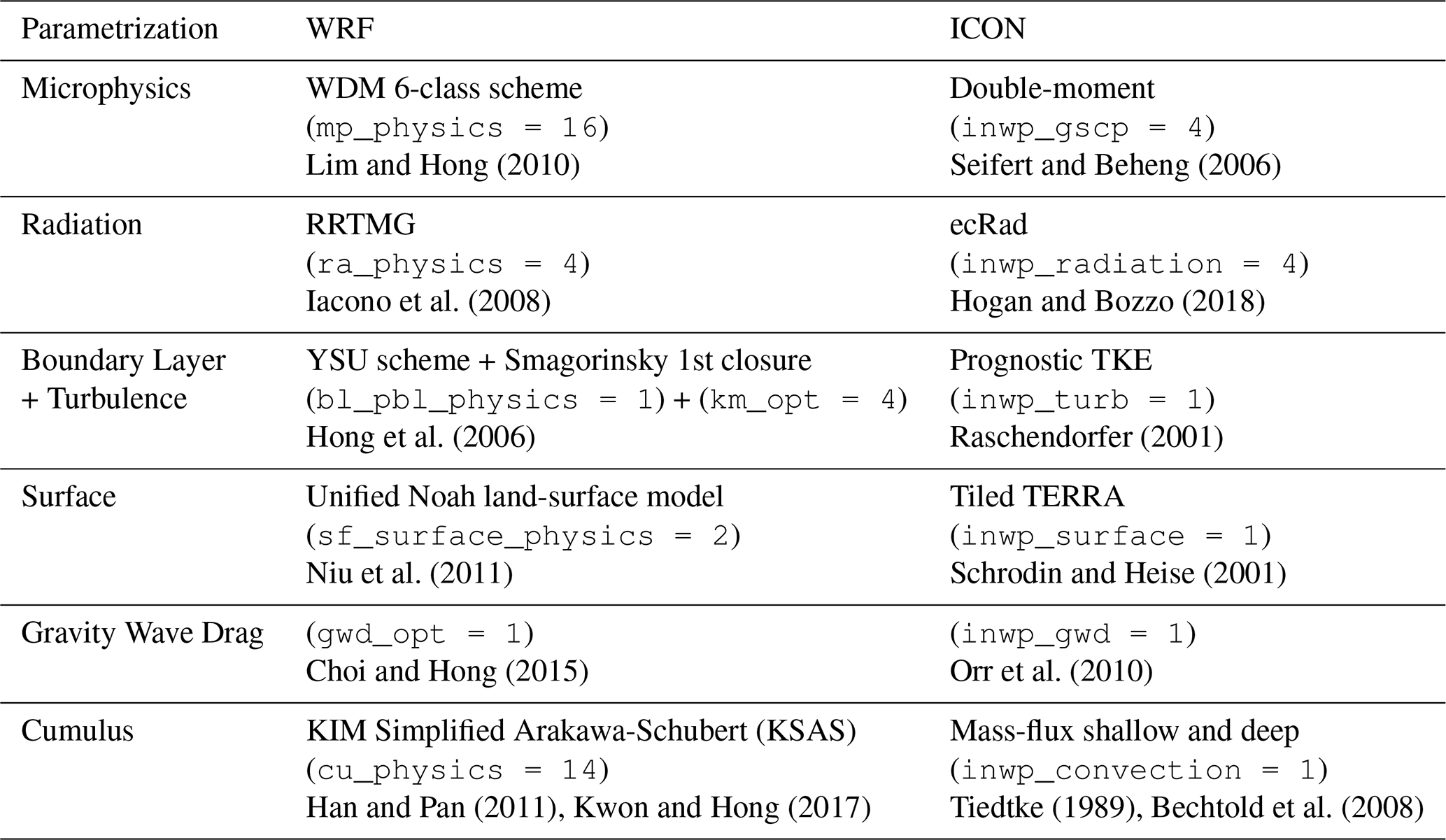
Despite the effort to balance the configurations for the two simulations as much as possible, the physical parameterization suites of WRF and ICON could not be fully harmonized, reflecting the independent development lineages of the two modelling systems (Table 1). For each physics category we retained each model's standard, operationally validated configuration rather than forcing an artificial correspondence that neither code is designed to support. The most consequential divergence concerns cloud microphysics: the WDM6 scheme (Lim and Hong, 2010) predicts number concentration only for the warm-rain species, retaining a single-moment treatment for the ice-phase hydrometeors, whereas the two-moment scheme (Seifert and Beheng, 2006) used in ICON prognoses both mass and number concentration across all hydrometeor categories, including the ice phase. Radiative transfer is likewise computed by conceptually distinct codes, with RRTMG (Iacono et al., 2008) following a correlated-k approach, in contrast to the more modular, multi-solver architecture of ecRad (Hogan and Bozzo, 2018). Boundary-layer turbulence differs in closure order: the non-local, first-order YSU scheme (Hong et al., 2006), paired with a first-order Smagorinsky closure for residual 3D mixing in WRF, compared to ICON's prognostic, 1.5-order TKE-based scheme (Raschendorfer, 2001). Surface exchanges are computed by the single-tile Unified Noah land-surface model in WRF (Niu et al., 2011), as opposed to the explicitly tiled TERRA scheme in ICON (Schrodin and Heise, 2001), which resolves sub-grid land-cover heterogeneity relevant to the complex coastlines of the Mediterranean basin. Gravity-wave drag is included in both configurations, though following distinct orographic formulations (Choi and Hong, 2015; Orr et al., 2010). Finally, convection is parameterized by mass-flux schemes of different heritage: the KIM Simplified Arakawa–Schubert scheme in WRF (Han and Pan, 2011; Kwon and Hong, 2017), versus the Tiedtke–Bechtold scheme in ICON (Tiedtke, 1989; Bechtold et al., 2008), the latter treating shallow and deep convection as explicitly separate regimes. These structural differences, intrinsic to the two model architectures, represent an additional, model-dependent source of uncertainty that should be considered alongside the dynamical and resolution-related aspects of the comparison discussed above.

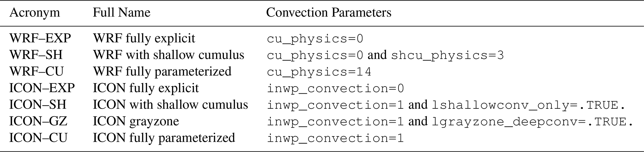
In addition, we are also testing the sensitivity to the convective schemes because the two models have differences in the choice of configuration. The following numerical experiments are performed:

• WRF explicit, i.e. no active convection parameterization (WRF–EXP),

• WRF fully parameterized calculation, both deep and shallow convection (WRF–CU),

• WRF independent shallow cumulus option WRF–SH (not tied to deep convection and GRIMS shallow cumulus from YSU group)

• ICON explicit, i.e. no active convection parameterization (ICON–EXP),

• ICON fully parameterized calculation, both deep and shallow convection (ICON–CU),

• ICON shallow cumulus option tied to deep convection (ICON–SH)

• ICON grayzone parametrization tied to deep convection, (ICON–GZ).

The grayzone parametrization used in ICON–GZ is a NWP-specific tuning of the deep convection scheme in order to reduce the activity of the convection scheme to just a bit more than pure shallow convection. It includes an increased entrainment rate for parcel ascent calculations and a modified CAPE closure in order to suppress widespread convective drizzle (Deutscher Wetterdienst, 2025).

A summary of the numerical experiments is in Table 2.

Table 2 Numerical experiments performed using WRF and ICON using several configurations.

3.2 Observations

Observation plays a key role in validating the results of numerical simulations, providing the necessary benchmark to assess their accuracy and realism. However, in meteorological events such as TLC Daniel, which evolved primarily over offshore regions, the spatial density and temporal frequency of available observations are markedly scarce. Therefore, any comprehensive validation effort is challenging. During the initial extra-tropical phase of the event, a reasonable number of surface pressure and wind measurements were available from several land-based meteorological stations, as well as from ships operating off the coast of Greece. Hence, a relatively reliable data set is available for the early development of the system. In contrast, during the following phase over the Ionian Sea, observational coverage became largely sparse. The situation is even more critical in Libya, where the number of official weather stations is limited and they are far from the area directly affected by the cyclone. These data were retrieved from official sources and used to estimate the sea-level pressure and wind at ground as mentioned in Hérincs (2023) and are drawn on the map to highlight the position of the data and the displacement from the center of the cyclone (Fig. 3a).

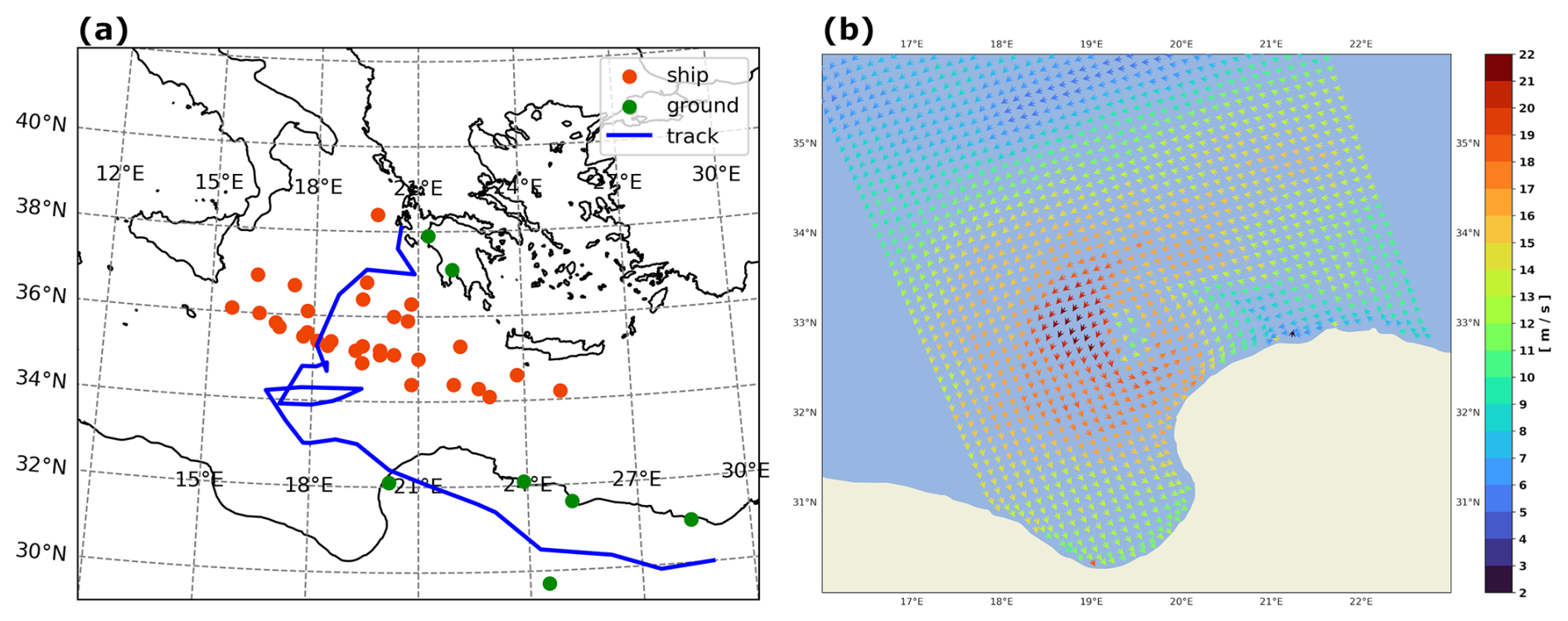
Figure 3 Available observations used for the estimation Central Sea Level Pressure and wind speed (Hérincs, 2023). (a) Location of ships, ground and buoys stations. In blue the track of the cyclone, in green the land-based stations, in orange ships and buoys. (b) The ASCAT MetOp-C wind speed measurements, at average time 20:02 UTC on 9 September 2023, wind arrows for direction in color shade according to wind speed.

In the open sea, intermittent satellite-based wind observations were available from the Advanced Scatterometer (ASCAT) instruments onboard the MetOp-B and MetOp-C satellites, operated by the European Organization for the Exploitation of Meteorological Satellites (EUMETSAT). These measurements are valuable for estimating surface wind fields on the sea side, but it is well known that ASCAT tends to underestimate wind speeds in regions affected by deep convection, as is typical in the case of tropical or tropical-like systems (Miglietta et al., 2025) (Fig. 3b).

During the genesis and extra-tropical phases, the dense National Observatory of Athens automatic network (NOANN/METEO) (Lagouvardos et al., 2017) provides high-resolution surface and rainfall observations. However, offshore over the open Ionian Sea and in Libya, there is a dramatic lack of ground-based observations. For the sake of consistency, we have decided to use satellite-derived precipitation estimates for the evaluation over the whole domain. During extreme weather events, Satellite-based rainfall products are recorded with sufficient accuracy, not only the amount of rainfall but also its spatial distribution (Kolios and Papavasileiou, 2024; Katsanos et al., 2024). In particular, data from the Integrated Multi-satellitE Retrievals for Global precipitation measurement (IMERG) (Huffman et al., 2023) product are used to evaluate the two-dimensional cumulative precipitation fields, offering a more complete representation of the atmospheric conditions during the peak of the event. The dataset refers to the “final” run v07 satellite-gauge product merged into half-hourly 0.1° × 0.1° (roughly 10 × 10 km nominal spatial resolution) fields.

IMERG Final incorporates gauge information only through a monthly climatological adjustment and underestimated the observed maxima over Thessaly during this event (Flaounas et al., 2025); model overestimates diagnosed over Greece against IMERG should hence be read as upper bounds.

3.3 Cyclone track

One of the interesting information for a cyclone is definitely the track, that is the path that the cyclone traces during its life. Therefore, an analysis of it is performed: first, the observed track is built and used as reference; then, the simulated one is computed based on the model results; finally, the distance between these two is computed.

3.3.1 Observed track

The observed track is obtained through the High Resolution Visible (HRV) images produced by the Spinning Enhanced Visible Infra-Red Imager (SEVIRI) Meteosat Second-Generation (MSG) satellite and provided by EUMETSAT. A Python algorithm is used to manually select the location of the center of the cyclone. For each available image, the algorithm acts as a graphical interface, showing the image and allowing the user to select the point where the pressure minimum is assumed to be located. This selection is made by selecting the center of the eye, where present, or the point of maximum convergence of the convective system. The longitude, latitude, and date are extracted from the selection. The temporal resolution of the track is set to 3 h and a nominal spatial resolution of 1 km, but with an uncertainty of about 15 km due to the difficulty in identifying the exact position of the cyclone center.

3.3.2 Tracking algorithm

For what concerns the tracks of the model simulations, an “ad hoc” algorithm is newly developed. Basically, the tracking technique consists of following the minimum mean sea level pressure. However, this can cause errors. The high-resolution simulations for deep convection events may develop a few deep pressure minima located beneath the most intense cells, which forces the algorithm to deviate by the deepest minimum. To overcome this issue, our algorithm is built by choosing the centroid of the cells with values of mean sea level pressure lower than the 5th percentile in a radius of 150 km from the previously detected cyclone center. To ensure the track toward the deepest minimum, this constraint is also applied to the geopotential levels between 900 and 800 hPa, to allow for good tracking even in a baroclinic atmosphere. The final result is an average of the individual minimum and centroid points. To ease the visual representation of the cyclone track a smoothing is applied using a 3 h moving mean window.

In order to evaluate the goodness of the simulated tracks, we use the mean error (μ), the standard deviation (σ) and the Root Mean Squared Error (RMSE) computed on the geodetic distance w.r.t. the observed track. Since the uncertainty on the observed track applies equally to all simulations and through the track, it does not affect the error evaluation of the configurations, but it is still taken into account while evaluating the statistical significance of the results.

3.4 Meteorological variables

To analyse this event, several models meteorological variables are used:

• Sea Level Pressure (SLP), both Mean SLP (MSLP) and Central SLP (CSLP), i.e. minimum MSLP at the center of the cyclone, which provide an indication of cyclone intensity; the observational data are drawn from Hérincs (2023), which relies on records from ships, buoys, and official weather stations, with the underlying trend then reconstructed by means of the UKMet analysis.

• Wind speed, at 10 m above ground, which can be compared with the Saffir-Simpson Hurricane Wind Scale (SSHWS) to estimate cyclone strength; the observational data are drawn from Hérincs (2023), which relies on records from ships, official weather stations and satellite data.

• Precipitations patterns, accumulated amount and location

The following parameters are analysed along the cyclone track as follows: time series are built for the CSLP and the 10 m maximum wind (MW10); the minimum pressure and the maximum wind are extracted at each timestep within a radius of 150 km of the cyclone center and plotted separately highlighting landfall and absolute extremes. Moreover, the simulated total accumulated precipitation over the whole duration of the event is compared with the IMERG one.

Model-minus-IMERG difference maps of the event-total precipitation, computed on the common verification grid (Fig. S4 in the Supplement), show that the leading error structure along the track is a displacement dipole rather than a uniform intensity bias. WRF overestimates accumulation over the Pindus slopes, ICON underestimates it on the southern flank of the cyclone, and the dipole amplitudes are smallest in the SH configurations of both models.

The Fractions Skill Score (FSS) is used to evaluate rainfall. Both observed and model rainfall are regridded in a common spatial domain. The FSS is defined as (Roberts and Lean, 2008):

$$\begin{array}{}\text{(1)}& {\mathrm{FSS}}_{\mathit{\tau }}=\mathrm{1}-{\displaystyle \frac{{\sum }_w{\left(p_{w,\mathit{\tau }}^{\mathrm{O}}-p_{w,\mathit{\tau }}^{\mathrm{S}}\right)}^{\mathrm{2}}}{{\sum }_w{\left(p_{w,\mathit{\tau }}^{\mathrm{O}}\right)}^{\mathrm{2}}+{\sum }_w{\left(p_{w,\mathit{\tau }}^{\mathrm{S}}\right)}^{\mathrm{2}}}}\end{array}$$

where τ is a fixed threshold, w is the dimension of the window, $p_{w,\mathit{\tau }}^{\mathrm{O}/\mathrm{S}}$ number of Observed/Simulated grid cells in the window w whose accumulated precipitation exceeds the value τ and ∑_w is the sum over all window sizes ranging from 1 cell to 171 cells (maximum extension equal to almost the entire domain). The following thresholds are defined:

• 6th percentile = 1 mm

• 50th percentile = 16 mm

• 85th percentile = 108 mm

• 95th percentile = 193 mm

• 99th percentile = 308 mm

• 99.9th percentile = 428 mm

The FSS evaluates the spatial overlap of fractional coverage between model and observations, ranging from 0 (complete mismatch) to 1 (perfect forecast). Because the score is symmetric, a low FSS value indicates a general mismatch in fractional coverage, which can stem equally from spatial displacement, over-forecasting, or under-forecasting. To rigorously assess the spatial scale at which a model becomes skilful, we employ the “useful scale” criterion introduced by Roberts and Lean (2008). A forecast is considered skilful when the FSS exceeds a target value defined as ${\mathrm{FSS}}_{\mathrm{useful}}=\mathrm{0.5}+f_{\mathrm{0}}/\mathrm{2}$, where f₀ is the domain-average fractional coverage of the observed event. Since f₀ is inherently very small for localized extreme precipitation (such as the upper percentiles analysed here), the target threshold is effectively FSS_useful≈0.5. The minimum window size required to reach this value represents the spatial scale at which the model provides a reliable precipitation forecast.

3.5 Physical processes of the event

3.5.1 Cyclone Phase Space Diagram (CPS)

The analysis of the physical mechanisms of the phenomenon is focused on the tropical characteristics of the cyclone. A kind of cyclone identity card can be created by exploiting the three-dimensional Cyclone Phase Space Diagram (CPS) developed by Hart (2003).

The three parameters used to describe the general structure of cyclones are the lower-tropospheric thermal asymmetry (B) and the thermal wind ($-V_{\mathrm{T}}^{\mathrm{L}}$), and the upper-tropospheric thermal wind ($-V_{\mathrm{T}}^{\mathrm{U}}$). The first phase space diagram generated is the storm-motion-relative thickness asymmetry (B vs. $-V_{\mathrm{T}}^{\mathrm{L}}$) identifying areas symmetric/non-frontal versus asymmetric/frontal. The second is the vertical derivative of the horizontal height gradient ($-V_{\mathrm{T}}^{\mathrm{U}}$ vs. $-V_{\mathrm{T}}^{\mathrm{L}}$) that describes the structure of cold- versus warm-core via the thermal wind relationship. The parameters are calculated according to Hart (2003) using values in a circular area around the center of the cyclone with a radius R=300 km.

Medicane-adapted CPS variants employ smaller radii and shifted layers (e.g., 100 km and 925–700–400 hPa; Picornell et al., 2014; Miglietta et al., 2025). A sensitivity test on ICON–SH, varying the radius between 100 and 500 km and testing both layer sets, shows that the numerical values of B, $-V_{\mathrm{T}}^{\mathrm{L}}$ and $-V_{\mathrm{T}}^{\mathrm{U}}$ fluctuate between setups while the effect sizes remain small (mean Cohen's d between −0.28 and 0.35), and that the adopted configuration (300 km, standard layers) lies near the centre of the tested ensemble (mean absolute z-score 0.24). The original Hart framework is retained for comparability with the existing literature on tropical and tropical-like cyclones. The coloured thresholds in Figs. 8–9 are indicative, qualitatively inspired by the SSHWS, and serve only as a visual aid for comparing simulations.

3.5.2 Temporal Annular Symmetric Mean (TASM)

The equivalent potential temperature (θ_e) is used to explore the internal structure of the cyclone during the tropical phase. This variable is used because it accounts for both dry potential temperature (sensible heating) and amount of water vapor (latent heating) and it is conserved along the process, making it a good tracer for humid air-masses and easily comparable at different heights.

Vertical cross-sections of θ_e are often employed to inspect the moist thermodynamic and warm-core structure of tropical and tropical-like cyclones (Emanuel, 2018; Miglietta and Rotunno, 2019). This approach is easy to use for tropical cyclones, where the symmetric structure is well defined and the required spatial resolution is not too high. However, when applied to TLCs in the Mediterranean, it is highly dependent on the direction of the cutting for the cross-section since symmetry is not so defined and the need for high-resolution simulations makes the field even more variable. For this reason, we used what we will call “Temporal Annular Symmetric Mean” (TASM). Assuming a symmetric cyclone structure, the horizontal field is divided into concentric circular coronas, centered on the cyclone's core and of thickness ΔR. Both θ_e and the wind speed are averaged within each corona for all levels, thus generating the Annular Symmetric Mean (ASM). To overcome the temporal dependence, the ASM is repeated for at least 8 consecutive time steps, including the absolute minimum of CSLP. This results in a TASM for a good indicative tropical-like period. The results are evaluated according to the known structure of Tropical Cyclones (Emanuel, 2018; Tous and Romero, 2011).

4 Results

4.1 Track

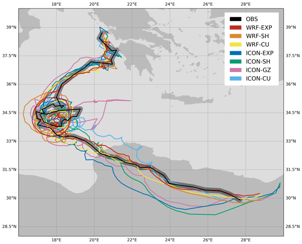
At first, the model tracks of the cyclone are compared with the observed one. They are shown in Fig. 4 with the following color code: WRF–EXP in red, WRF–SH in orange, WRF–CU in yellow; ICON–EXP in blue, ICON-SH in green, ICON-GZ in magenta, ICON-CU in light-blue. The observed track is the black line. Overall, all simulations reproduce the general path of the cyclone, which moves from the Ionian Sea to Libya and then turns eastward towards Egypt. However, there are significant differences in terms of spatial and temporal accuracy.

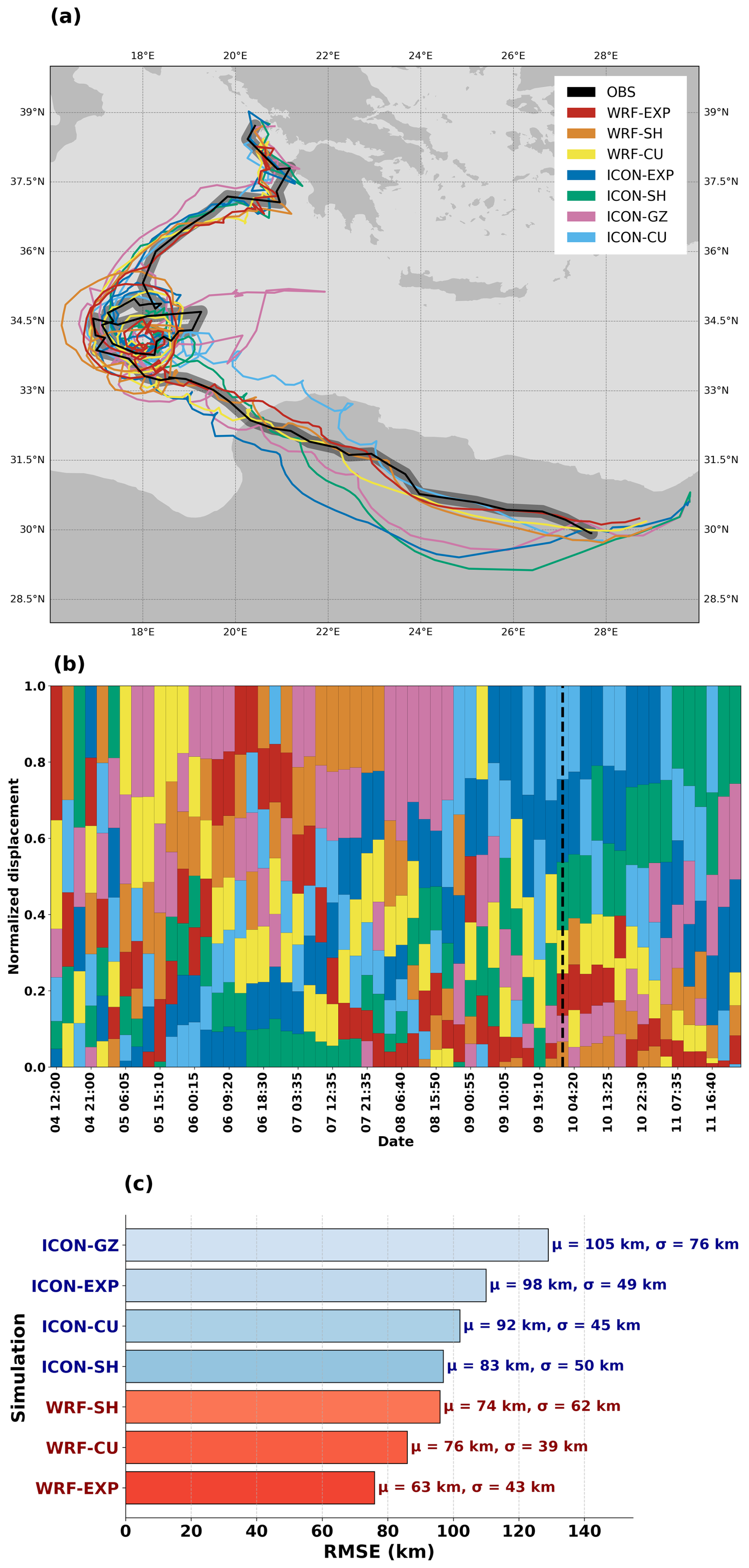
Figure 4 (a) The cyclone tracks for: WRF–EXP in red, WRF–SH in orange, WRF–CU in yellow; ICON–EXP in blue, ICON–SH in green, ICON–GZ in magenta, ICON–CU in light-blue, observed track is the black line with a shadowed buffer indicating the estimated 15 km error. (b) Normalized error in km w.r.t. the observed track; bars are stacked vertically for each timestep, i.e. lower is better; same colors of panel (a). (c) RMSE, mean value and standard deviation of each simulation.

To objectively evaluate the goodness of the models track the mean error and RMSE are computed using as reference the observed HRV track. The WRF–EXP simulation shows the best performance, with a mean error of 63 km and a RMSE of 76 km (Fig. 4c). The cyclone is accurately tracked throughout its life cycle, with a slight eastward bias during the landfall phase. The WRF–SH simulation has a mean error of 74 km and a RMSE of 96 km. The cyclone is correctly tracked in the early phase, but it deviates significantly during the landfall phase, with a westward bias. The WRF–CU simulation has a mean error of 76 km and a RMSE of 86 km. The cyclone is poorly tracked in the early phase, with a northward bias, but the track improves during the landfall phase, with a slight eastward bias.

The ICON–EXP simulation has a mean error of 98 km and a RMSE of 110 km. The cyclone is well tracked in the early phase, but it deviates significantly from the observed track during the landfall phase, with a westward bias. The ICON–SH simulation has a mean error of 83 km and a RMSE of 97 km. The cyclone is poorly tracked in the early phase, with a northward bias, but improves during the landfall phase, with a slight eastward bias. The ICON–GZ simulation has a mean error of 105 km and a RMSE of 129 km. The cyclone is poorly tracked throughout its life cycle, with a significant northward bias. The ICON–CU simulation has a mean error of 92 km and a RMSE of 102 km. Again, the cyclone is poorly tracked in the early phase, with a northward bias, but it improves during the landfall phase, with a slight eastward bias.

While WRF exhibited a lower mean track error compared to ICON, rigorous significance testing accounting for serial correlation demonstrates that this difference is not statistically significant (p=0.28), being largely overshadowed by the substantial variability along the cyclone life cycle. In particular, WRF better reproduces the barotropic conditions (TL phase) than the baroclinic ones, whereas ICON seems to be better in the baroclinic storm phase (Fig. 4b). The choice of cumulus parameterization also affects the performance. Although explicit and shallow cumulus schemes yielded lower absolute mean errors in our sample compared to fully parameterized schemes, these improvements are statistically indistinguishable once serial correlation is accounted for. Therefore, a strict ranking of individual configurations based solely on track error cannot be robustly supported for this specific event.

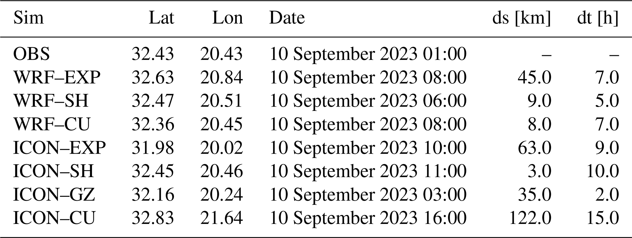
A detailed analysis of the landfall phase shows that ICON–SH has the smallest spatial error, but a time delay of 10 h. The best time synchronization is provided by ICON–GZ, but with a spatial error of 35 km. The best overall simulation appears to be WRF–SH, which has a spatial error of only 9 km and a delay of 5 h. The other simulations show larger displacements, ranging from 35 to 122 km in space and from 2 to 15 h in time. A summary of this analysis is shown in Table 3.

Table 3 Summary of landfall data including location, date, displacements in space and in time w.r.t. satellite observation of landfall.

4.2 Meteorological variables

The comparison among the models meteorological variables and the observed one is now presented. The time series of CSLP and MW10 along the cyclone track are shown in Fig. 5a and b respectively. The observed time series (OBS) are retrieved from Hérincs (2023). Hérincs (2023) reconstructs the pressure evolution from buoy, ship and land-station records (shown in our Fig. 3a), cross-checked against the UK Met Office analysis, and derives the wind estimates from station and satellite data. We cross-validated these estimates against ECMWF ReAnalysis v5 (ERA5) (Hersbach et al., 2023a) and a higher-resolution Copernicus European Regional Reanalysis (CERRA) (Schimanke et al., 2021). The comparison (Fig. S9) shows a consistent temporal evolution across datasets, with two systematic differences. First, the Hérincs pressures are slightly lower than the reanalysis values, while the absolute minimum is similar. Second, in Hérincs (2023) the minimum occurs offshore before landfall, whereas the reanalyses place it several hours later, over land. We consider the offshore timing more consistent with the expected behaviour of a marine warm-core cyclone: over the sea the vortex continues to extract latent and sensible heat from the surface, while the low surface roughness limits frictional spin-down; both supports are cut off at landfall. The land-based minimum in the reanalyses likely reflects their coarse effective resolution and the scarcity of in-situ MSLP data over the southern Ionian, which limit the analysed depth of a small-core vortex until it reaches the better-observed coast. For the wind, the reanalyses show a positive bias of up to 10 m s⁻¹ with respect to Hérincs (2023), but the temporal trend is consistent. On this basis we retain the Hérincs (2023) dataset as a qualitative reference for the temporal evolution. All simulations manage to reproduce the general trend of the variables, with a decrease in CSLP and an increase in MW10 during the most intense phase of the cyclone. However, there are significant differences in terms of intensity and timing.

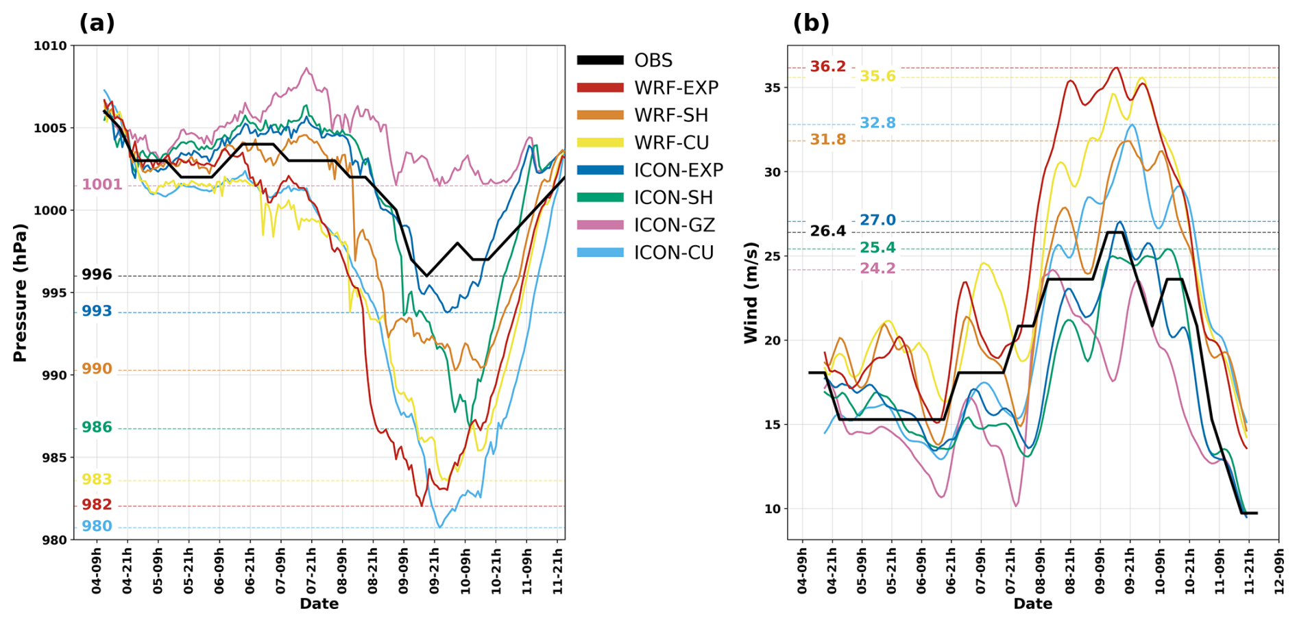
Figure 5 Timeseries of the cyclone variables: (a) CSLP every 6 h for observation and 1 h for the simulations; (b) maximum wind speed within a radius of 150 km from cyclone center every 6 h for observation and 1 h for simulations using a 6 h running mean. WRF–EXP in red, WRF–SH in orange, WRF–CU in yellow; ICON–EXP in blue, ICON–SH in green, ICON–GZ in magenta, ICON–CU in light-blue. Reference behaviour of the observations in black.

To be noticed, the observed minimum CSLP of 996 hPa may be an overestimation due to the lack of data in the area where the cyclone reached its peak intensity. In fact, the Benina International Airport, which is the closest available observation to the cyclone, recorded a surface pressure of 984 hPa at an elevation of approximately 132 m above sea level and reported a sea level pressure of 999.3 hPa at 00:00 UTC on 10 September 2023, more than 50 km away from the cyclone's center. Similar considerations can be made for the wind speed. The ASCAT Metop-C passing over the cyclone at 20:02 UTC on 9 September 2023, shows a maximum wind speed of 22 m s⁻¹, but it is known that scatterometer measurements tend to underestimate the real value in situations of deep convection (Miglietta et al., 2025).

As a reference of strength of the cyclone, according to the SSHWS, an hurricane can be classified in category C1 if the maximum sustained wind speed is between 33 and 42 m s⁻¹. While according to the observed value from ASCAT it should be categorized as a Tropical Storm.

During the most intense phase of the cyclone, significant differences are found among the model simulations in terms of the minimum central sea level pressure (CSLP) (Fig. 5a) and the maximum 10 m wind speed (MW10) (Fig. 5b). For what concerns the WRF simulations: WRF–EXP produced the lowest minimum CSLP of 982 hPa, with MW10 approximately 36.2 m s⁻¹ around the cyclone center during its maximum intensity; WRF–SH yielded a higher minimum CSLP of 990 hPa, with MW10 of 31.8 m s⁻¹, while the WRF–CU configuration produced a minimum CSLP of 983 hPa, with MW10 of 35.6 m s⁻¹.

Similarly, for the ICON simulations: ICON–EXP produced a minimum CSLP of 993 hPa and MW10 of 27 m s⁻¹; ICON–SH yielded 986 hPa with MW10 of 25.4 m s⁻¹; ICON–CU reached a minimum CSLP of 980 hPa, accompanied by MW10 of 32.8 m s⁻¹, representing the most intense results among the ICON configurations. In contrast, the ICON–GZ setup exhibited the weakest system, with a minimum CSLP of 1001 hPa and MW10 of 24.2 m s⁻¹.

Overall, the WRF configurations tend to produce lower CSLP values and larger MW10 speeds compared to the ICON ones, indicating a generally more intense cyclone representation. While the shallow parameterization for WRF decreases both the intensity and the strength of the cyclone, on the contrary for ICON it tends to allow a greater deepening in terms of CSLP while decreasing MW10. Fully parameterized configurations increase both the intensity and strength of the cyclone, likely by creating deep convection cells that rotate in phase around an axis. This is particularly true for ICON, where ICON–CU reaches the lowest CSLP and the strongest MW10; while in WRF the WRF–CU experiment reaches intensities similar to those of WRF–EXP.

The observed CSLP minimum is used only as a qualitative reference for the temporal evolution; the quantitative statements in this section only compare the simulations with one another.

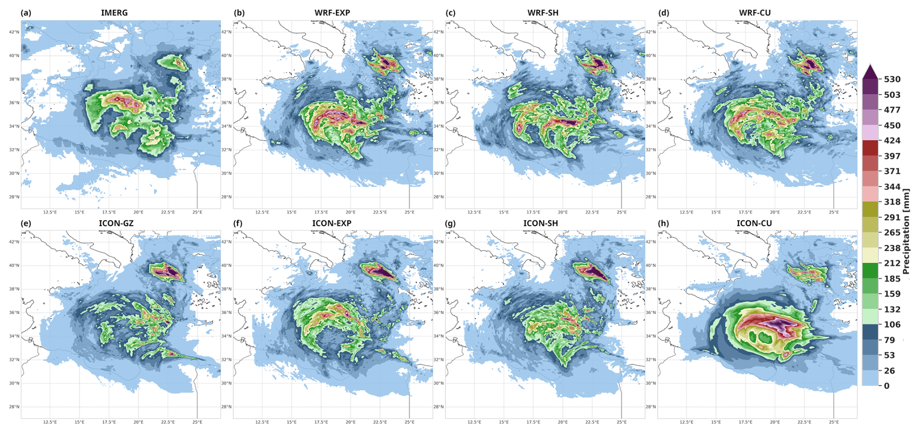
Figure 6 Accumulated total precipitations during the event (4–12 September 2023). (a) Observations from IMERG, (b) WRF–EXP, (c) WRF–SH, (d) WRF–CU, (e) ICON–GZ, (f) ICON–EXP, (g) ICON–SH, (h) ICON–CU. Color shades as for FSS percentile thresholds in Fig. 7.

The total accumulated precipitation during the whole event (4–12 September 2023) is shown in Fig. 6. All simulations are able to reproduce the general pattern of the precipitation, with a maximum over the Ionian Sea and the northwestern Greece. However, there are significant differences in terms of quantity and location.

The mean accumulated precipitation per grid cell is an indicator of the total rainfall in the domain. This quantity has been computed as the spatial average of the event-total accumulated precipitation over the full analysis domain, on the common verification grid shared by both models and IMERG. The following values are obtained: 31.4 mm for IMERG, 34.8 mm for WRF–EXP, 33.3 mm for WRF–SH, 34.3 mm for WRF–CU, 29.3 mm for ICON–EXP, 27.0 mm for ICON–SH, 39.1 mm for ICON–CU, 23.9 mm for ICON–GZ. These values show that the precipitation is systematically larger for the WRF experiments, while the ICON simulations are generally drier, although ICON–CU produces the largest accumulated rainfall value and ICON–GZ is markedly drier than the other configurations.

The spatial distribution of the precipitation shows that WRF produces (Fig. 6b, c, d) a pattern consistent with observations, highlighting the three circular structures related to the different precipitation phases. On the other hand, ICON–SH shows (Fig. 6g) a remarkable improvement with respect to the other ICON configurations (Fig. 6e, f, h).

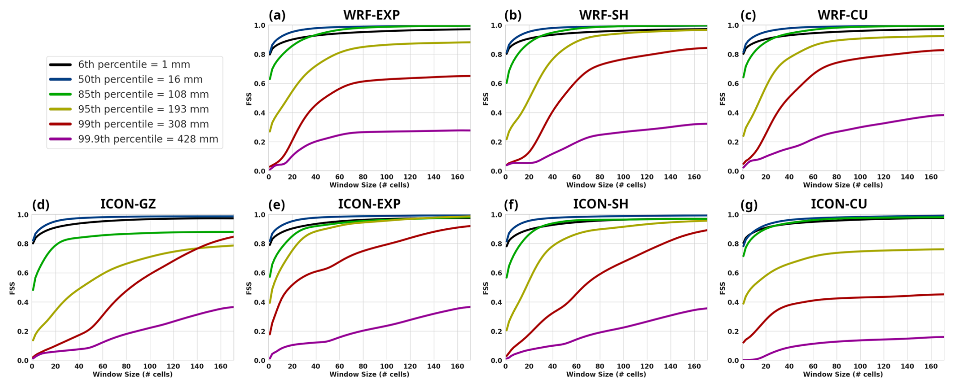
Figure 7 FSS scores for each simulation with respect to IMERG. On the x-axis the window size used for the FSS computation. Color shades based on percentiles consistent with Fig. 6.

The FSS is now used for a quantitative analysis of the simulated precipitation fields. Assessing the FSS as a function of the neighbourhood window size highlights the specific spatial capabilities of each simulation. High FSS values at small window sizes indicate an accurate spatial localization of the precipitation. Conversely, when the FSS only rises at larger window sizes, it implies that the model captures the overall precipitation frequency but suffers from significant displacement errors at the grid scale. At low thresholds, all models exhibit high skill scores, rapidly exceeding the FSS_useful≈0.5 criterion even at small spatial scales (Fig. 7a–d, black and blue lines). Noticeable differences emerge starting from the 85th percentile, where the fully parameterized ICON–CU scheme achieves the best performance at finer scales (Fig. 7g, green line). However, as the threshold rises to the 95th percentile, the best grid-scale result for WRF is obtained with the SH configuration, while ICON–EXP demonstrates the highest skill among the ICON simulations at small window sizes (Fig. 7b and e, yellow line). The 99th and 99.9th percentiles highlight the most dramatic discrepancies among the experiments. WRF–SH is the only configuration achieving an FSS > 0 at the native grid scale (1×1) for both extreme thresholds (Fig. 7b, red and violet lines), indicating some exact spatial overlap for extreme local accumulations. Conversely, ICON–CU yields the lowest overall FSS at these extremes (Fig. 7g, violet line), reflecting a severe mismatch in fractional coverage. ICON–SH and ICON–EXP, while exhibiting displacement errors at the native grid scale, show a sharp increase in skill at larger window sizes, ultimately attaining the highest overall FSS values (Fig. 7e and f, red lines). This indicates that although these setups struggle to pinpoint the exact location of extreme cells, they successfully reproduce the correct fractional coverage of extreme precipitation over broader areas, reliably crossing the FSS_useful threshold at synoptic scales. Overall, taking both peak accumulations and spatial scales into account, ICON–EXP attains the most robust FSS performance.

Examining the minimum skillful (FSS≥0.5) window sizes across configurations and thresholds reveals that nearly all simulations achieve skill at the grid scale (1 grid-cell) up to the 85th percentile, whereas none reach skillfulness at the 99.9th percentile threshold. The main differences emerge at the 99th percentile threshold, where ICON–EXP achieves skillfulness at the smallest window size (19 grid-cells), followed by WRF–CU (41 grid-cells), WRF–EXP and WRF–SH (49 grid-cells), ICON–SH (67 grid-cells), and ICON–GZ (85 grid-cells). ICON–CU fails to reach an FSS threshold of 0.5. The frequency distributions of event-total precipitation, evaluated on the common verification grid (Figs. S5–S6), show agreement with FSS scores.

4.3 Physical structure of the cyclone

In this section, the tropical characteristics of the cyclone are analysed to the aim of understanding its physical structure. The CPS diagrams for the lower symmetry (B vs. $-V_{\mathrm{T}}^{\mathrm{L}}$ plane) and core characteristics ($-V_{\mathrm{T}}^{\mathrm{U}}$ vs. $-V_{\mathrm{T}}^{\mathrm{L}}$ plane) are shown respectively in Figs. 8 and 9. All simulations show a general similar behaviour in the B vs. $-V_{\mathrm{T}}^{\mathrm{L}}$ plane, with an initial phase of decreasing asymmetry and increasing warm core until reaching a maximum value of $-V_{\mathrm{T}}^{\mathrm{L}}$. During this tropical-like phase the symmetry tends to oscillate around zero, keeping the structure in the expected range.

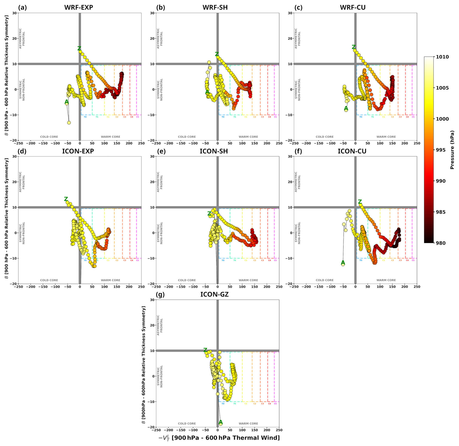
Figure 8 CPS B vs. $-V_{\mathrm{T}}^{\mathrm{L}}$ plane: core lower tropospheric symmetry. The letters A to Z indicate the cyclone life cycle, with time moving forward along the trajectory, from the labelled A to Z. The shading of the markers corresponds to the intensity of the cyclone (in hPa), with light color as the weakest and dark color as the most intense. Rainbow dashed lines indicate the thresholds for the cyclone phase classification.

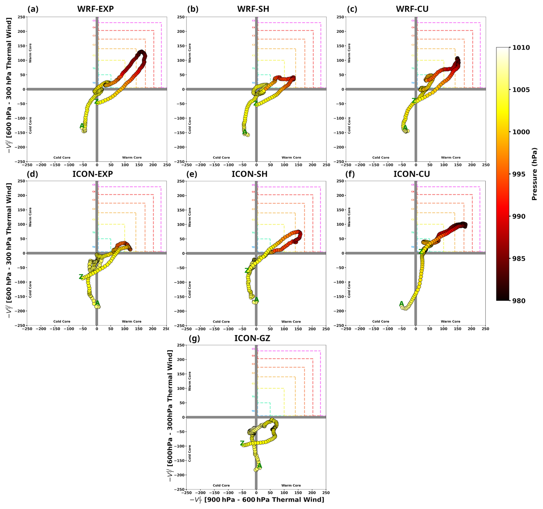
Figure 9 CPS $-V_{\mathrm{T}}^{\mathrm{U}}$ vs. $-V_{\mathrm{T}}^{\mathrm{L}}$ plane: core temperature and deepness. The letters A to Z indicate the cyclone life cycle, with time moving forward along the trajectory, from the labelled A to Z. The shading of the markers corresponds to the intensity of the cyclone (in hPa), with light color as the weakest and dark color as the most intense. Rainbow dashed lines indicate the thresholds for the cyclone phase classification.

But differences are found for the two models: WRF shows (Fig. 8a–c) a gradual increase in core temperature ($-V_{\mathrm{T}}^{\mathrm{L}}$) while oscillating in symmetry until the dissipation stage, which is characterized by a rapid decrease of the core temperature and an increase in the asymmetry. On the other hand, ICON tends to warm up the core later than WRF but more rapidly (Fig. 8d–f). Moreover, as expected from the track analyses, ICON–GZ does not develop a Tropical-Like Cyclone, keeping a cold core and disorganized structure (Fig. 8g).

Also for the $-V_{\mathrm{T}}^{\mathrm{U}}$ vs. $-V_{\mathrm{T}}^{\mathrm{L}}$ plane, all simulations show a similar behaviour, with an initial phase of contemporaneous warming in the upper and lower levels until reaching a peak in upper right section, followed by a phase of cold and shallow core. However, there are significant differences in terms of balance in the lower and upper warming. WRF–SH and ICON–EXP seem to have difficulties in transferring energy to the upper layers resulting in a colder core in the $-V_{\mathrm{T}}^{\mathrm{U}}$ axis (Fig. 9b and d, respectively). As previously pointed out ICON–GZ does not even reach the threshold to enter a tropical-like classification (Fig. 9g).

To better understand the structure of the cyclone produced by the two models, a further analysis is performed using the Temporal Annular Symmetric Mean which allows for exploring the internal structure of the cyclone during the tropical phase. The typical structure of a vertical cross–section of θ_e for a Tropical Cyclone reveals a pronounced warm column all around the center extending from the lower troposphere to approximately 200 hPa. Usually at the 500 hPa there is a relative minimum due to subsidence and reduced moisture that inhibit deep convection creating the eye of the cyclone. Around it, larger values of θ_e form a sort of pillars representing the vigorous ascent and strong diabatic heating of the eye wall. Beyond it, θ_e decreases steadily with distance from the center (Emanuel, 2018).

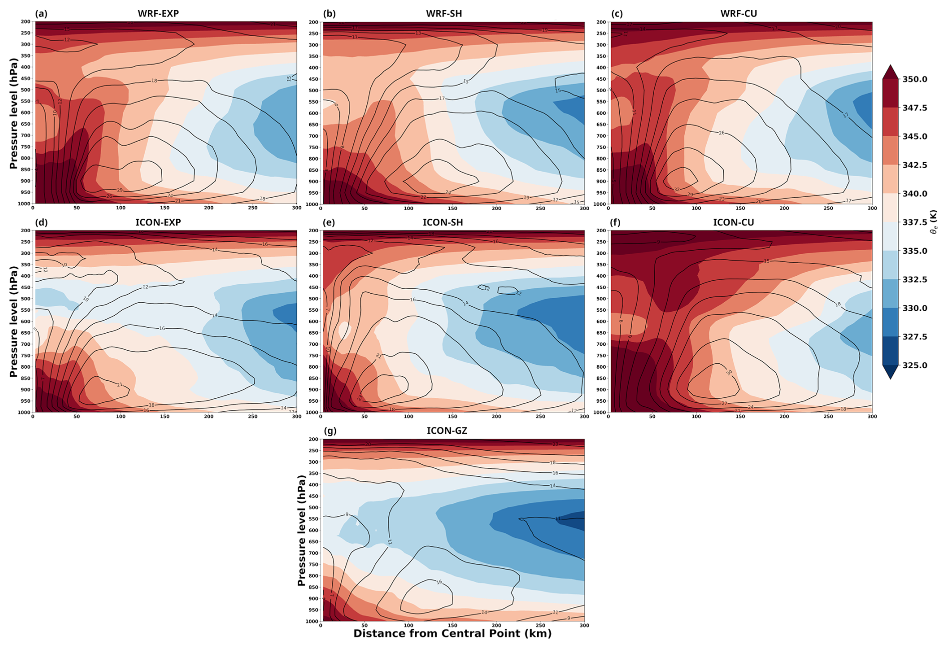
Figure 10 TASM: wind speed (m s⁻¹, black contours) and equivalent potential temperature (K, filled contours) for the simulations using different cumulus parameterizations. Each panel is averaged over 8 timesteps before landfall. (a) WRF–EXP from 10 September 2023 01:00 to 08:00 UTC. (b) WRF–SH from 9 September 2023 23:00 UTC to 10 September 2023 06:00 UTC. (c) WRF–CU from 10 September 2023 01:00 to 08:00 UTC. (d) ICON–EXP from 10 September 2023 03:00 to 10:00 UTC. (e) ICON–SH from 10 September 2023 04:00 to 11:00 UTC. (f) ICON–CU from 10 September 2023 09:00 to 16:00 UTC. (g) ICON–GZ from 9 September 2023 20:00 UTC to 10 September 2023 03:00 UTC.

The simulations of both models show maximum values of θ_e in the lower levels, close to the cyclone center, increasing up to 800 hPa and gradually decreasing horizontally away from it (Fig. 10). This indicates strong diabatic heating in the lower troposphere near the minimum SLP and the extraction of heat from the sea. However, there are significant differences among the simulations in terms of vertical extent and horizontal distribution.

WRF–EXP and WRF–CU show (Fig. 10a and c, respectively) a well-defined warm core extending up to approximately 300 hPa, with a clear eye wall structure and a relative decrease of θ_e in the range of 650–600 hPa and a horizontal extension of a few tens of km. The wind contours are packed near the eyewall reaching maximum values at 50–100 km far from the center at 900 hPa. Similarly for WRF–SH (Fig. 10b) but producing a less pronounced eyewall and a relative minimum of θ_e around 550 hPa. The wind contours are less packed than for WRF–EXP, but they are still following the eyewall, the maximum values can be found at 100–150 km far from the center at 900 hPa.

ICON–EXP shows (Fig. 10d) a warm core extending up to 550 hPa, with poor connection with the upper layers. Wind contours are packed approaching the cyclone center with maximum values 50-100 km from the center below 900 hPa. ICON–SH shows (Fig. 10e) a warm core extending up to 300 hPa, with an eyewall extremely close to the center and a relative minimum of θ_e around 625 hPa, but not aligned with the central axis. The wind contours are packed in the first tens of kilometers from the center with maximum values at 50–100 km at 900 hPa. ICON–CU shows (Fig. 10f) values of θ_e reaching larger values than the other ICON simulations, with similar characteristics, except for a deep intrusion of θ_e from the upper layers, suggesting the presence of intense cells that rotate organized around a minimum pressure, but without the development of a real tropical-like cyclone. ICON–GZ shows (Fig. 10g) a very weak cyclone structure with a thick layer of low θ_e values from 650 to 400 hPa and wind contours distant from each other with almost half the values compared to other simulations.

These results suggest that the ICON simulations are more sensitive to the cumulus scheme used than the WRF ones.

5 Discussion and Conclusion

In this study, an inter-comparison of high-resolution simulations of Medicane Daniel between two leading weather forecasting models, WRF and ICON, is presented. The objective is to understand the role of convective parameterization at the ≈ 2 km “grayzone” resolution and the different representations of the event by the two models. In order to ensure a robust comparison, the following model settings were constrained to be similar: domain, vertical discretizations, initial and lateral boundary conditions (IC/LBC) and physical parameterizations. Despite the effort to balance the configurations for the two simulations as much as possible, the physical parameterization suites of WRF and ICON could not be fully harmonized, reflecting the independent development lineages of the two modelling system. These structural differences, intrinsic to the two model architectures, represent an additional, model-dependent source of uncertainty.

The experiments reveal that the transition from a baroclinic disturbance to a tropical-like cyclone (TLC) is primarily driven by sub-grid scale convection. Although both models capture the broad life cycle of Daniel, significant differences in wind intensity, surface pressure, accumulated precipitation and internal structure highlight the strong control exerted by physical parameterizations, even within convection-permitting regimes.

Both models show differences in the storm structure that vary during the stages of the storm. ICON demonstrates good accuracy during the initial extratropical phase, likely benefiting from its global-model heritage and efficient representation of large-scale baroclinic dynamics. In contrast, WRF exhibits a reduced track error and greater consistency among configurations during the mature tropical-like phase, suggesting that its mesoscale-focused physics may be better tuned for the diabatic processes dominating TLC Daniel maintenance in these simulations.

The inclusion of a shallow convection (SH) parameterizationin this experiment proved to be important for both models, significantly improving landfall accuracy near Benghazi compared to fully explicit (EXP) or fully parametrized (CU) configurations. This suggests that at ≈ 2 km resolution, the explicit computation of shallow non-precipitating clouds is insufficient at least for the Daniel case. Instead, parameterizing these clouds is fundamental to modulate boundary layer moisture flux and preconditioning the environment for organized deep convection, thereby refining the storm's trajectory.

The sensitivity to the shallow-convection treatment admits a consistent physical reading. At 2 km grid spacing, non-precipitating shallow cumuli are not resolved. The shallow schemes (GRIMS in WRF, the shallow-only Tiedtke–Bechtold mode in ICON) vent boundary-layer moisture into the lower free troposphere; the sub-cloud layer dries, grid-scale moisture convergence weakens and the onset of resolved deep convection is delayed, so that latent heating is released over a wider area rather than in a few grid-point updrafts. This mechanism is consistent with the weaker but better organised cyclone in WRF–SH, with the improved localisation of extreme rainfall (Fig. 7b) and with the smoother eyewall structure in the TASM diagnostics (Fig. 10). In the CU experiments, instead, the parameterized deep heating acts on top of the resolved convection and feeds a positive feedback between heating and central pressure fall, consistent with the over-intensification of ICON–CU. This interpretation is diagnostic; a quantitative attribution would require moisture-budget and heating-profile analyses beyond the scope of this study.

Numerical simulations reveal a systematic bias regarding the intensity of the cyclone: WRF consistently produces deeper central sea-level pressures (CSLP) and stronger maximum 10 m winds (MW10) than ICON. Physically, this is explained by the different vertical structures identified in the Temporal Annular Symmetric Mean (TASM) diagnostics. The WRF configurations generate a vertically coherent warm core that extends up to 300 hPa, with a distinct eyewall-like θ_e maximum. This vertical alignment favours barotropic intensification and reduces tilt-induced ventilation, enhancing hydrostatic pressure falls through the thermal wind relationship. In contrast, ICON–EXP exhibits a shallow warm anomaly, largely confined below 550 hPa, which limits the depth-integrated thickness anomaly and subsequent surface pressure deepening. The ICON–GZ (grayzone) experiment represents a critical failure mode, as it over-damps convective development and prevents the transition to a diabatic, Wind-Induced Surface Heat Exchange (WISHE)-like maintenance mechanism. This suggests that, at this resolution, the GZ parameterization suppresses the updraft generation too much without compensating for the missing energy with advective flow, inhibiting the development of deep convection necessary for the tropical transition. Moreover, an over-intensification of the cyclone is obtained by WRF–CU and ICON–CU simulations, which schemes trigger an unrealistic positive feedback loop between latent heat release and pressure deepening, leading to extreme CSLP values. However, the internal structure of the cyclone differs; while WRF–CU maintains a concentrated eye-wall structure, ICON–CU exhibits a broader moisture distribution and lacks a distinct structural “pillar”, suggesting that while deep-convection schemes can produce intense pressure drops, they may struggle to realistically organize inner-core dynamics at high resolution.

These structural discrepancies are mirrored in the precipitation analysis. WRF tends to over-produce precipitation, while ICON under-produces it with respect to IMERG data. The Fraction Skill Score (FSS) analysis indicates that WRF–SH uniquely attains skill on the grid scale for extreme rainfall thresholds. This suggests that a hybrid approach, allowing explicit deep convection while retaining shallow parameterization, enhances the localization of convective cores without over-smoothing updrafts. Overall, the EXP and SH configurations retain the largest FSS values for both models, particularly ICON–EXP.

The results must be interpreted in light of Daniel's intrinsic peculiarity as a long-lived, multi-stage Mediterranean cyclone. Unlike systems that rapidly attain a mature structure, Daniel evolved through a prolonged sequence of physically distinct stages: an initial baroclinic phase, a tropical transition and a mature TLC phase. This temporal persistence across heterogeneous regimes makes the event a stringent benchmark for testing model physics, requiring a single framework to represent large-scale forcing and mesoscale convective organization with comparable skill.

Several factors limit the generalization of these findings. First, the lack of high-frequency, in-situ surface observations over the open Mediterranean necessitates reliance on satellite-derived tracks and reanalysis for validation. Second, as a single-case design, these results may be specific to Daniel's unique dynamical pathway, especially given the high variability reported in the literature for other medicanes. Furthermore, the role of microphysics interacting with convection and air-sea feedback (e.g., sea spray and wave-induced drag) remains an unquantified source of uncertainty that may account for some intensity differences.

The present findings sit consistently within the medicane sensitivity literature. The first-order control of the convective treatment on track and intensity confirms the single-case results of Miglietta et al. (2015), and the benefit of a dedicated shallow-convection treatment at kilometre scale agrees with Saraceni et al. (2023). The large spread among configurations, with no single setup performing best across all phases and metrics, mirrors the multi-physics results of Ricchi et al. (2017, 2019) and Pytharoulis et al. (2018). Daniel departs from most previously studied events in its prolonged, multi-stage evolution, which stresses model physics across heterogeneous regimes within a single integration. Accordingly, the operational indications given below are to be read as case-specific: findings established for Daniel under the present configurations, findings consistent with prior studies, and hypotheses that remain to be tested across additional cases and initialization times.

For Daniel under the present configurations, retaining a shallow-convection parameterization improved some aspects of the simulation, especially for selected precipitation and structure metrics. Here, a hybrid approach using shallow convection schemes acts as a “bridge”, allowing models to resolve organized deep convection while parameterizing necessary smaller-scale mixing. However, the failure of ICON–GZ and the over-intensification of CU schemes underlines that scheme portability cannot be assumed. At this resolution, the solution is governed by the combined action of physical parameterizations and the numerical framework; therefore, the same physical option may not be dynamically equivalent across different models due to differences in discretization, diffusion and vertical coordinates. It follows that each model requires dedicated and finely tuned calibration.

Part of the systematic WRF–ICON contrast may stem from the unmatched physics rather than from the convective treatment. The single-moment ice phase in WDM6, as opposed to the fully two-moment Seifert–Beheng scheme, plausibly alters the vertical distribution of latent heating and hence the warm-core depth diagnosed in the TASM; the non-local YSU mixing, compared with ICON's prognostic-TKE closure, modulates the boundary-layer moisture supply and the near-surface wind maxima. Cross-model statements in this study should hence be read as differences between full model configurations, whereas causal statements about the convection scheme are restricted to the within-model experiments.

The large sensitivity found in this work reinforces the need for case-specific forecast strategies. For long-lived systems like Daniel, researchers should not assume that a single “optimal” setup is robust across all phases; instead, an in-depth sensitivity analysis should be performed on a case-by-case basis. Future research should expand to multi-physics ensembles to assess the coupling between boundary layer schemes and the successful shallow-convection setups identified here. In physically heterogeneous areas such as the Mediterranean basin, model deficiencies during the transition from baroclinic to tropical-like regimes may propagate into substantial errors in rainfall distribution, amount and landfall timing. Hence, early-warning systems should not rely exclusively on nominal horizontal resolution, but also on demonstrated model skill for the specific class of high-impact events being targeted. Additionally, investigating the role of Gravity Wave Drag (GWD) in modulating the upper-level PV streamer's interaction with the surface vortex could provide further insights into the predictability of the transition phase. Finally, high-resolution coupled atmosphere–ocean simulations are needed to determine how SST feedbacks modulate vertical warm-core depth and whether such feedbacks could mitigate the intensity biases observed in WRF and ICON.