Detection and global climatology of two types of spatio-temporal clustering of extratropical cyclones

The swift succession of multiple extratropical cyclones during a short period of time is often associated with weather extremes and characterised by a strong atmospheric jet and enhanced baroclinicity. While several diagnostics exist to detect cyclone clustering, they mostly focus on regional assessments or rely on statistical measures that do not allow for a direct association with individual storms. Hence, we introduce a global detection for spatio-temporal clustering of extratropical cyclones, inspired by the original idea of cyclone families by Bjerknes and Solberg, in which individual cyclones follow a similar track. We further subdivide cyclone clusters into two types, a sequential type and a stagnant type. The former is associated with cyclones that follow each other over a minimum distance, whereas the stagnant type requires a proximity over time, while not moving much in space.

We find that spatio-temporal cyclone clustering is most frequent along the storm tracks, with more cyclone clustering during winter compared to summer. The majority of cyclone clustering occurs just south of the main storm tracks in the Atlantic and Pacific basins. In the Southern Hemisphere, most cyclone clustering is found in the South-Indian Ocean.

Sequential type cyclone clustering is associated with stronger cyclones compared to non-clustered cyclones, while for the stagnant type this intensity difference is less pronounced. This effect is strongest for the North Atlantic and North Pacific, while clustered cyclones in the South Indian Ocean are generally not much stronger. The cyclone intensity within the sequential type does not decrease during a cluster, while in contrast ensuing cyclones of the stagnant type are significantly weaker than the respective primary cyclone. This suggests that these two types of spatio-temporal cyclone clustering are dynamically different.

1 Introduction

The rapid succession of extratropical cyclones during a short period of time is often associated with European weather extremes, such as extensive wet spells (Moore et al., 2021) and strong wind gusts yielding large economic losses (Priestley et al., 2018). The idea that several cyclones follow a similar track dates back to the concept of cyclone families by Bjerknes and Solberg (1922). However, given that not all periods adhere to the Bjerknes and Solberg model of cyclone families, the term serial cyclone clustering has been introduced to define these periods (Dacre and Pinto, 2020). To automise the detection of cyclone clustering, algorithms have either been based on regional definitions using cyclone frequencies (Pinto et al., 2014; Priestley et al., 2017) or on a statistical analysis of storm recurrence (e.g. Mailier et al., 2006; Vitolo et al., 2009). While the former uses a local time constraint, which is especially meaningful for regional impact studies, the other statistically assesses unusual spatial occurrence. Given the separation of space and time for individual cyclone tracks in these two approaches, we introduce an approach using the spatio-temporal vicinity of cyclone tracks to define cyclone clusters. Our method can readily be applied globally and allows for a separation into different types of clusters based on the type of space-time proximity, enabling a more dynamical assessment of the detected clusters and characteristics of the clustered cyclones.

Based on the idea that cyclones occur more regularly over time in some regions, Mailier et al. (2006) defined cyclone clustering (serial clustering in their paper) using a dispersion diagnostic, comparing local occurrence of cyclones with a random Poisson process. They refer to a region as underdispersive when the monthly cyclone occurrence at a particular location is less variable than expected from a Poisson process. In contrast, a region is overdispersive when cyclone occurrence is more variable compared to a Poisson process. The latter is associated with cyclones clumping together in time as clusters and is mainly found at the exit regions of the North Atlantic and North Pacific storm tracks. Similar algorithms have been applied by Kvamstø et al. (2008); Vitolo et al. (2009); Pinto et al. (2013); Economou et al. (2015). Future changes in this dispersion statistic are generally small and have large uncertainties (Economou et al., 2015). A downside with this statistical definition, however, is that it defines clustering in a relative sense. To investigate the dynamical mechanisms behind cyclone clustering, it would be preferable to be able to diagnose why certain cyclones follow a similar track, posing the need to detect the specific cyclones that are part of a cluster. The dispersion diagnostic, however, does neither quantify how many cyclones and clusters pass at a particular location nor identify which cyclones are part of a particular cluster.

Another set of diagnostics for serial clustering of cyclones counts the number of cyclones at a particular location during a defined period of time (Pinto et al., 2014; Priestley et al., 2017; Bevacqua et al., 2020). For example, Priestley et al. (2017) defined clustering off the coast of western Europe as the occurrence of at least 4 cyclones in a period of seven days within a radius of 700 km around that location. Using composites of clustered events in this way, they found that clustering at the storm track exit is related to a strong extended jet, flanked by double sided Rossby wave breaking. A similar algorithm was used by Bevacqua et al. (2020), but using a maximum temporal distance between cyclones of one day, instead of counting cyclones in the seven day running mean. While these algorithms detect individual cyclones as part of a cluster, they rely on a locally confined definition of cyclone clustering as well as the pre-selection of the most intense cyclones.

Priestley et al. (2020b) extended the method of Priestley et al. (2017) to distinguish if detected cyclones form along the trailing cold front of a previous cyclone. This allows to distinguish between primary and secondary cyclones, which is a useful classification, as clustering is often associated with secondary cyclogenesis, while other mechanisms include the role of the eddy driven jet, Rossby wave breaking, and downstream development (Pinto et al., 2014). Priestley et al. (2020b) found that about 50 % of the cyclones are clustered along the Atlantic storm tracks. Although this algorithm is less local than the previous algorithms, it relies on both a frontal as well as a cyclone detection. Detecting fronts relies on several choices and is thus sensitive to the chosen variable for detection (Thomas and Schultz, 2019). Furthermore, this algorithm cannot detect clustered cyclones that form due to other mechanisms than secondary cyclogenesis.

Synoptically, clustering over the Atlantic is often associated with strong, elongated jets and secondary cyclogenesis along trailing cold fronts of preceding cyclones (Pinto et al., 2014; Priestley et al., 2017; Weijenborg and Spengler, 2020). Stronger jets correspond to higher baroclinicity, which explains that clustered storms tend to be more intense (Vitolo et al., 2009). However, given that several cyclones follow a similar track, in general one would expect that the baroclinicity is reduced after each cyclone. Therefore, one needs to explain how this baroclinicity is maintained. Given the importance of latent heating for the maintenance of baroclinicity (Hoskins and Valdes, 1990; Papritz and Spengler, 2015), Weijenborg and Spengler (2020) proposed that cyclone clustering could be caused by latent heating along trailing cold fronts. Ideally a clustering algorithm should thus detect cyclone clustering events to investigate if this is a preferred cyclone development mechanism.

There have also been attempts to investigate the similarity of tracks of extratropical cyclones, for example Blender et al. (1997) used k-means clustering based on the cyclone displacement relative to its genesis location. They divided North-Atlantic cyclone tracks into zonal, north-east moving, and stationary types. While this definition of clustering ensures that different cyclones follow tracks in a similar direction, it does not take the temporal component into account. Therefore, this definition puts all cyclones traveling in a zonal direction in the same cluster, independent if they occur shortly after each other or not. Individual cyclone tracks in such a cluster can thus be dynamically unrelated if they do not also occur in a certain proximity in time.

The diagnostics outlined above thus either define serial clustering with a local criteria for proximity in time or use statistical measures that cannot distinguish between individual cyclone tracks. However, to be able to disentangle the dynamical mechanisms of different types of cyclone clustering, irrespective of their geographic location, and potential differences of cyclone characteristics therein, there is a need for an algorithm that ideally:

• checks if cyclone tracks are in space-time proximity over a considerable amount of distance and/or time

• detects which cyclones are members of a specific cluster

• is unbiased with respect to the clustering mechanism

• does not require a strict intensity threshold on cyclones

• is applicable globally

Such an algorithm allows to address new questions about cyclone clustering, such as: What are preferred regions for spatio-temporal clustering of cyclones? Are there regions where cyclones cluster more locally in time without necessarily moving much in space, or where they cluster in space and time, i.e., they move along similar paths? Are the different types of cyclone clustering associated with different mechanisms and do the cyclones of the respective types feature different dynamic characteristics?

Motivated by these questions, we introduce an algorithm that defines cyclone clustering based on spatio-temporal vicinity of cyclones tracks. Our proposed algorithm can be applied globally, which also helps to alleviate the sparse focus on clustering in the North Pacific and the Southern Hemisphere (Dacre and Pinto, 2020). We also introduce two types of clusters, one resembling the original idea of Bjerknes and Solberg (1922) with cyclones following a similar track over a longer distance and another where cyclones do not move much over their lifetime. We present a global climatology of both types and discuss differences in intensity between clustered and non-clustered cyclones as well as differences between cyclone intensity within the different types of clusters.

2 Data and Methodology

We use the ERA-Interim reanalysis from the European Centre for Medium Range Weather Forecasts (ECMWF) (Dee et al., 2011), which is available at a triangular truncation of T255 with a 6-hourly time interval providing analyses at 00:00, 06:00, 12:00, and 18:00 UTC. We interpolated the data onto a 0.5° grid and use the mean sea level pressure to detect and track extratropical cyclones. Preliminary tests using ERA5 (Hersbach et al., 2020) basically yielded very similar results (not shown).

We use the University of Melbourne cyclone detection and tracking algorithm (Murray and Simmonds, 1991a, b). The algorithm detects cyclones as maxima in the Laplacian of the mean sea level pressure and tracks them over time using a nearest-neighbourhood method together with the most probable direction of propagation (Murray and Simmonds, 1991a, b; Michel et al., 2018). We use the same parameters as in Tsopouridis et al. (2021) and select cyclone tracks that last at least 24 h. However, in contrast to Tsopouridis et al. (2021), we do not pre-select any threshold on storm intensity and do not apply any requirements on a minimum distance travelled by cyclones. We decided against these additional criteria, because we want to investigate if clustered cyclones are stronger compared to non-clustered cyclones. We do not include a distance criterion to detect all cyclones belonging to the stagnant type. To minimize the influence of orography, we discard cyclones located above 1000 m.

2.1 Detection of spatio-temporal clustering of extratropical cyclones

Conceptually, spatio-temporally clustered cyclones follow each other for a significant distance and/or time. Hence, for every pair of cyclone tracks we first check if they are close enough to each other in space and time (See Fig. 1). We check if the spatial distance between pairwise points along two tracks is within δx_local of one Rossby Radius of deformation ($L_{\mathrm{R}}=NH/f_{\mathrm{0}}$) and within a temporal period δt_local of 36 h (indicated by the red dots in Fig. 1a). The Rossby radius of deformation is a measure of the wavelength of maximum growth for baroclinic instability (Holton, 2004) and therefore sets the typical size of an extratropical cyclone. The choice of 1.5 d is roughly the median time passed between the occurrence of mid-latitude cyclones in the North Atlantic and North Pacific storm track regions in winter (not shown).

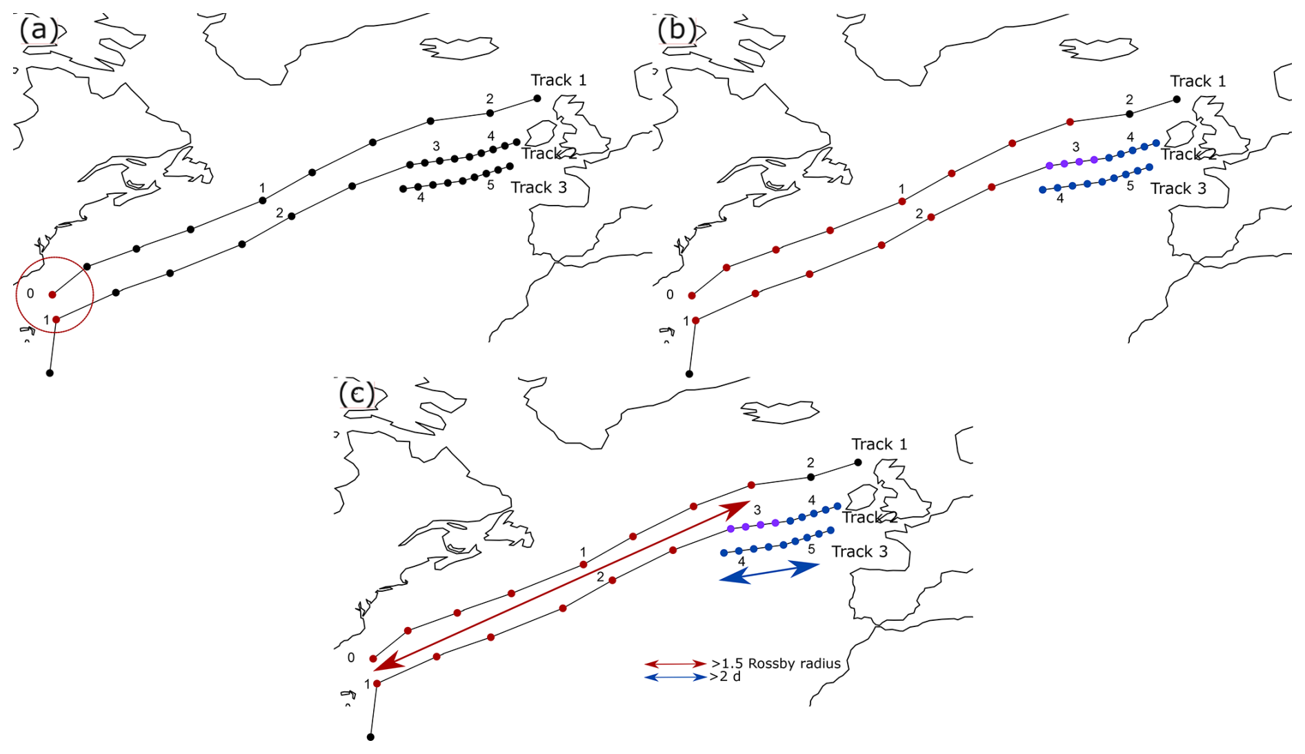
Figure 1 Schematic of spatio-temporal cyclone clustering detection. Black lines indicate three different cyclone tracks. Time in days since track 1 started is indicated by the timestamp next to each point. (a) Red radius indicates the distance threshold (Rossby radius of deformation) for one example point along track 1. (b) All points connected according to the criteria for the local space-time proximity are indicated by coloured points, with red points indicating a connection between track 1 and 2, and blue points indicating a connection between track 2 and 3, and purple points along track 2 are connected to both track 1 and 2. (c) Indication of the overlap in space (red arrow) and time (blue arrow) used in the second step of the algorithm. In this example, track 1 and 2 satisfy the length overlap criterion, while tracks 2 and 3 satisfy the time overlap criterion.

The approach described in Fig. 1a is very similar to other approaches detecting cyclone clustering. The main difference is that instead of only checking for local proximity of two cyclone tracks, we check for every pair of cyclone track points along two tracks if they are close together in space-time (coloured dots in Fig. 1b). In this first step, we only determine if two individual cyclones have a space-time proximity. In a second step, we assess the overlap between the identified cyclone couples traveling along a similar track in space δx_overlap and/or time δt_overlap (coloured dots in Fig. 1b).

The overlap distance is defined as the maximum distance between all cyclone couples in step 1, measured by the great circle distance between the first and last red dot in Fig. 1c. Similarly, the time overlap is defined as the total time elapsed between the first and last red dot in Fig. 1c. For all the connected points in step 1, we check if this maximum distance between them is either larger than 1.5 Rossby radius or that the temporal difference between them is more than 2 d. If either one of the two conditions is satisfied, the two cyclone tracks are connected as a cluster. The final step is combining these uniquely connected cyclone tracks, where each cyclone track in a cluster is connected to at least one other cyclone track, but not to any other cyclones outside the cluster (see Fig. 1c).

We choose a length overlap δx_overlap of at least 1.5 Rossby radius to have a minimum length of overlap significantly longer than the typical size of a cyclone. The time overlap δt_overlap of 2 d comprises a significant part of the cyclone lifetime. One could also have chosen slightly less strict thresholds, e.g. 1 Rossby radius and 1.5 d. However, while not qualitatively altering the results, these choices would lead to extremely long clusters, especially in the Southern Hemisphere (not shown). A further argument to choose the more strict parameters is to prevent that cyclones from different clusters end up in the same cluster. We tested the sensitivity by changing both the space-time proximity, as well the overlap thresholds. When altering these thresholds, the absolute frequencies of detected clusters changes, but there are no qualitative changes for the regions where clustering is most abundant. Our overlap thresholds are maybe on the lower end, though this allows to detect a larger variety of clusters, enabling the investigation of dynamical differences among the clusters.

Using the above method, we obtain all cyclone clusters, regardless if cyclones follow each other over a long distance or an extensive period of time. However, as the two types of clusters might be dynamically different, we distinguish between them and present climatologies for each category. We refer to these as the sequential type and stagnant type, dependent on if they fulfill the length or time criterion, respectively. We explicitly exclude the length criterion for the stagnant type, because they should represent clusters that do not move much in space. However, the sequential clusters might still satisfy the time criterion. For the schematic example in Fig. 1c, tracks 1 and 2 form a sequential type cluster, while tracks 2 and 3 are part of a stagnant cluster.

The sequential type is close to the cyclone families described by Bjerknes and Solberg (1922), though we do not specifically require that cyclones have to form on the same (polar) front. The stagnant type, on the other hand, represents cyclones that mainly cluster in time and that do not travel a significant distance along a similar track. As an individual cyclone can be simultaneously part of a sequential and a stagnant type cluster, there is a chance for double counting cyclones. For example, in Fig. 1, cyclone 2 is part of both a sequential as well a stagnant cluster. Hence, the cyclone track densities of sequential and stagnant type clustered cyclones are not additive and the sum can thus be larger than the density of all clustered cyclones.

As in Priestley et al. (2020b), we define cyclones that are not part of a cluster as “solo” cyclones. We compare both differences in location as well as in intensity between solo and clustered cyclones. To distinguish between primary and secondary cyclones, cyclones are ordered by the first time step they are connected with any cyclone in that cluster (coloured dots in Fig. 1). This time step might be different than the genesis location. For example, the first time step for track 2 in the example in Fig. 1 is not “clustered”.

To test the hypothesis that clustered cyclones are stronger, we use the maximum Laplacian of the mean sea level pressure in a small 1.25° radius around the cyclone centre during its lifetime to define the cyclone strength (similar as in Tsopouridis et al., 2021 and Michel et al., 2018). As the geostrophic relative vorticity is inversely proportional to the Coriolis parameter, and therefore the latitude ϕ, we normalise the Laplacian of the mean sea level pressure with sin (ϕ).

We choose the maximum of the normalised Laplacian of the mean sea level pressure instead of minimum pressure, as it is directly related to the geostrophic vorticity and thus the strength of the wind speed associated with a cyclone. Qualitatively, however, the results are not sensitive to this choice, given that cyclones with a larger Laplacian of mean sea level pressure are commonly associated with a deeper minimum in pressure. Furthermore, we define the intensity of a cluster using the maximum normalised Laplacian of mean sea level pressure of the strongest cyclone in a cluster. The results are qualitatively similar when choosing the mean intensity of cyclones in a cluster (not shown).

3 Climatology of clustered cyclone tracks

3.1 Winter

The occurrence of clustering in winter generally aligns with the climatological storm tracks for both the North Atlantic as well the North Pacific with clustered cyclones occurring about 10 %–14 % (Fig. 2b). In contrast, very few clustered cyclones are found in the Mediterranean and Barents Sea. While this is similar to Priestley et al. (2020a), though with slightly lower absolute values, our findings are in contrast to Mailier et al. (2006), who detected serial clustering mostly at the storm track exits. This difference is mainly due to our diagnostic determining absolute number of clustered storms, which is highest along the storm tracks. The dispersion diagnostic from Mailier et al. (2006), on the other hand, determines irregularities in the occurrence of cyclones in a given month, which is highest at the storm track exit, where the variability of the location of the jet is largest (Woollings et al., 2010).

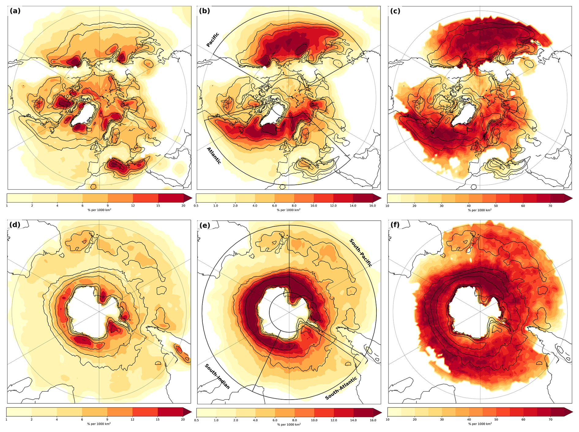
Figure 2 Cyclone densities defined as the fraction of time steps with a cyclone occurring per unit area of 1000 km² area. (a) Density of solo cyclones (not clustered) for DJF in the Northern Hemisphere. (b) and (c) as (a), but for clustered cyclones and Fractional density of clustered cyclones, respectively (shading). (d)–(f) as (a)–(c), but for JJA in the Southern Hemisphere. Black boxes in (b) and (e) indicate chosen regions in Sect. 4, and black contours in each panel indicate climatological storm tracks of all cyclones (contours at 10 %, 15 % & 25 % per 1000 km²).

The method of Priestley et al. (2017) uses a threshold of having at least 4 cyclones in a 7 d running of cyclone occurrence to detect cyclone clusters, which gives similar results in the storm tracks region if applied globally (see top left panel in Fig. S1), even when only using the more intense cyclones (see top right panel Fig. S1). When only retaining the most extreme cyclones, the signal shifts towards the exit of the storm track (see lower panel of Fig. S1). Hence, the reason that the frequency of cyclone clustering is highest at the end of the storm tracks for the Priestley et al. (2017) algorithm is due to the concomitant choice of a specific region as well as a threshold on cyclone intensity.

In contrast to the clustered cyclones, solo cyclones occur more regularly at other regions, e.g. at the storm track exit, the Barents Sea, and the Mediterranean Sea (Fig. 2a). Moreover, there are several additional regions where solo cyclones occur more regularly in the North Atlantic: in the lee of the Rocky mountains and over the Mediterranean sea. Priestley et al. (2020b) identified similar regions with high solo cyclone density, though with less solo cyclones around the Norwegian coast. Reason for this difference is most likely that they detect much fewer cyclones in this region in general (compare to their Figs. 3 and 4). In the Pacific basin, solo cyclones occur more often at the storm track exit.

The fraction of cyclone track densities associated with clustered cyclones in the Northern Hemisphere is about 50 % to 60 % of the total number of cyclone track densities (see Fig. 2c). Priestley et al. (2020b) detected cyclone families, consisting of primary and secondary cyclones, with the latter forming along the cold front of a primary cyclone. Even though our algorithm does not a priori detect secondary cyclones, the fractional track densities of up to 50 % to 60 % over North Atlantic in Priestley et al. (2020b) are similar. This indicates that a large part of our detected clusters most likely also form upstream of antecedent cyclone development.

In the North Pacific, the fractional density of clustered storms is slightly higher than in the North Atlantic. Highest fractional densities are found just south of the main storm tracks in both the North Atlantic and North Pacific (see Fig. 2c). Moreover, the fractional densities are oriented less northward compared to the climatological storm tracks, especially in the North Atlantic. This indicates that clustering occurs more often for more zonally oriented storm tracks, which is also the case for cyclone clustering associated with secondary cyclogenesis (Priestley et al., 2020b). However, we also find large clustering frequencies along the Norwegian coast at the storm track exit in the North Atlantic.

There are two main genesis regions in the North Atlantic for clustered cyclones, firstly near the Gulf Stream, and secondly in an area near Greenland (not shown). These genesis regions are partly similar to Priestley et al. (2020b), who found that cyclones forming due to secondary cyclogenesis mainly have genesis in these regions. In the North Pacific, genesis occurs generally more often on the western side of the basin over the Kurushio region (not shown). This indicates that clustered cyclones travel over the entire basin in the North Atlantic and North Pacific.

For the Southern Hemisphere winter season, cyclone cluster densities are highest in a small band around Antarctica, with the highest densities over the South Indian Ocean (Fig. 2e). Absolute numbers of clustering are higher compared to the Northern Hemisphere, which is partially due to higher cyclone densities in general. The fraction of clustered cyclones is about 60 %–75 %, which is comparable to the Northern Hemisphere (Fig. 2f). Furthermore, the genesis region is less clear compared to the Northern Hemisphere, with genesis of clustering mainly occurring in the same band as the storm tracks (not shown). Solo cyclones mainly occur along the coast of Antarctica, as well as between Australia and New Zealand.

The sequential-type clusters occur all over the North Atlantic and North Pacific regions, but relatively more at the entrance and just south of the storm tracks (Fig. 3a). In contrast, the stagnant type occurs more at the storm track exit in the North Atlantic and North Pacific as well as more to the north of the main storm tracks compared to the sequential type (Fig. 3b). Moreover, we detect more cyclones of this type in the North Pacific.

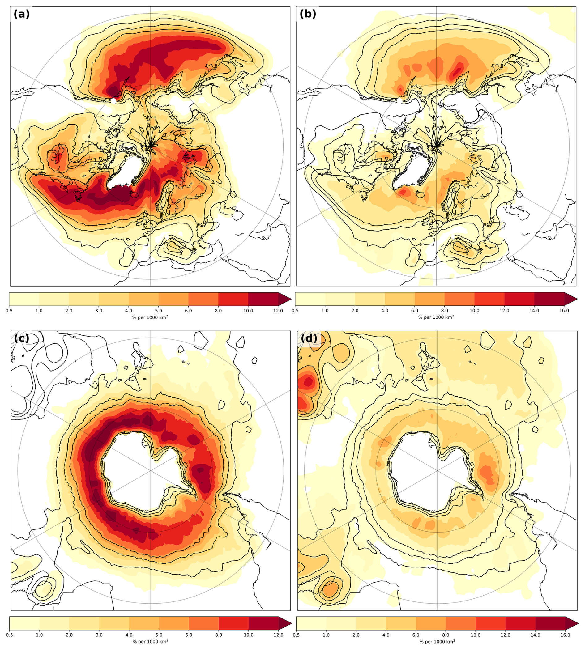
Figure 3 Densities for (left) sequential type and (right) stagnant type cyclone clusters for (top) Northern Hemisphere and (bottom) Southern Hemisphere for the respective winter season. Shading denotes fraction of times of a clustered cyclone at a location in a 1000 km² area. Black contours indicate clustered densities (at 2 %, 4 % and 6 % per 1000 km²)

In contrast, for the Southern Hemisphere, absolute numbers of stagnant type clustered cyclones are small (Fig. 3d). While sequential type clustered cyclones frequencies are about 6 %–12 % along the storm tracks (Fig. 3c), stagnant clustered cyclones frequencies are only 1 % to 4 %. The latter also occur frequently in subtropical regions, such as northwestern Australia, most likely demarcating the prevalent heat low in this location (Lavender, 2017), and around Madagascar.

3.2 Summer

For summer, the frequency of clustered storms in the Northern Hemisphere is significantly reduced and shifted to the western side of the basin, consistent with weaker storm tracks during summer (compare Figs. 2b and 4b). While Mesquita et al. (2008) found a northward shift of cyclones, especially on the western side of the basins, this is not evident for clustered cyclones in the Northern Hemisphere (Fig. 4b and c). Genesis is also slightly shifted to the west with less genesis of clustered cyclones in the lee of Greenland (not shown). For the Southern Hemisphere, there are no larger differences in the occurrence of clustered cyclones between summer and winter (compare Figs. 2e–f and 4e–f).

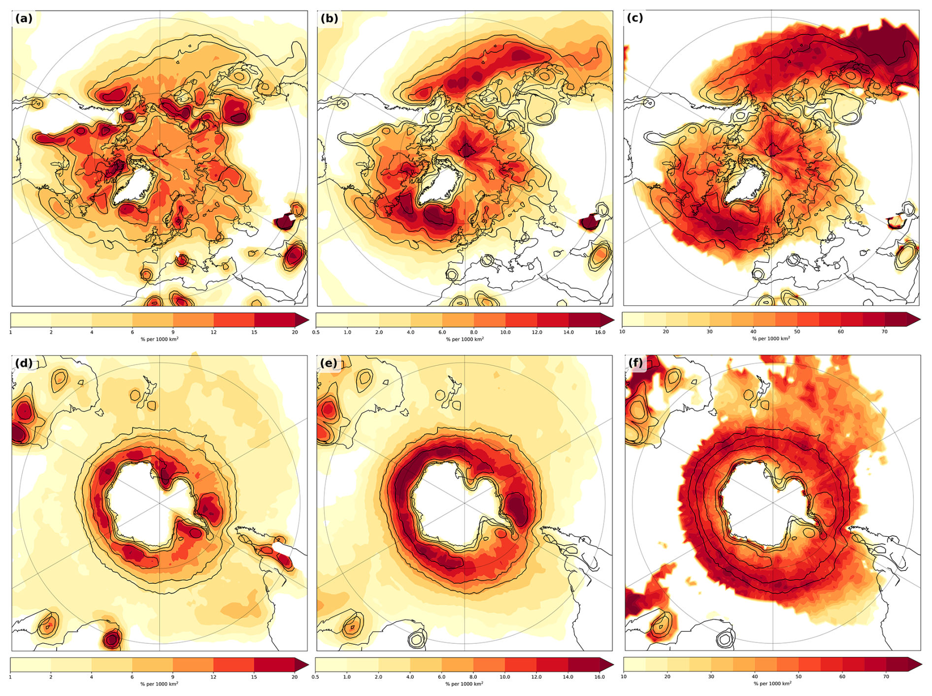
Figure 4 As Fig. 2, but for the respective summer seasons.

Solo cyclones in summer occur mainly within the storm tracks, suggesting a westward shift compared to winter (compare Figs. 2a and 4a). The shift to the west is less clear in the Southern Hemisphere (compare Figs. 2d–f and 4d–f), but densities for clustered cyclones are higher in the South Atlantic compared to further east in the South Indian Ocean.

The different cluster types are reduced in summer, with a stronger reduction in the sequential type (compare Figs. 3a–b and 5a–b). This is intuitive, as the jet strength is significantly reduced in summer, which mainly appears to affect the frequency of the sequential-type clusters (Fig. 5a). Furthermore, there is a shift towards the western side of the basins in the North Atlantic and North Pacific. However, for the stagnant clusters, cyclone densities are similar to winter. For the Southern Hemisphere, there is a decrease in the sequential-type clusters and a small increase in stagnant clusters (compare Figs. 3c–d and 5c–d).

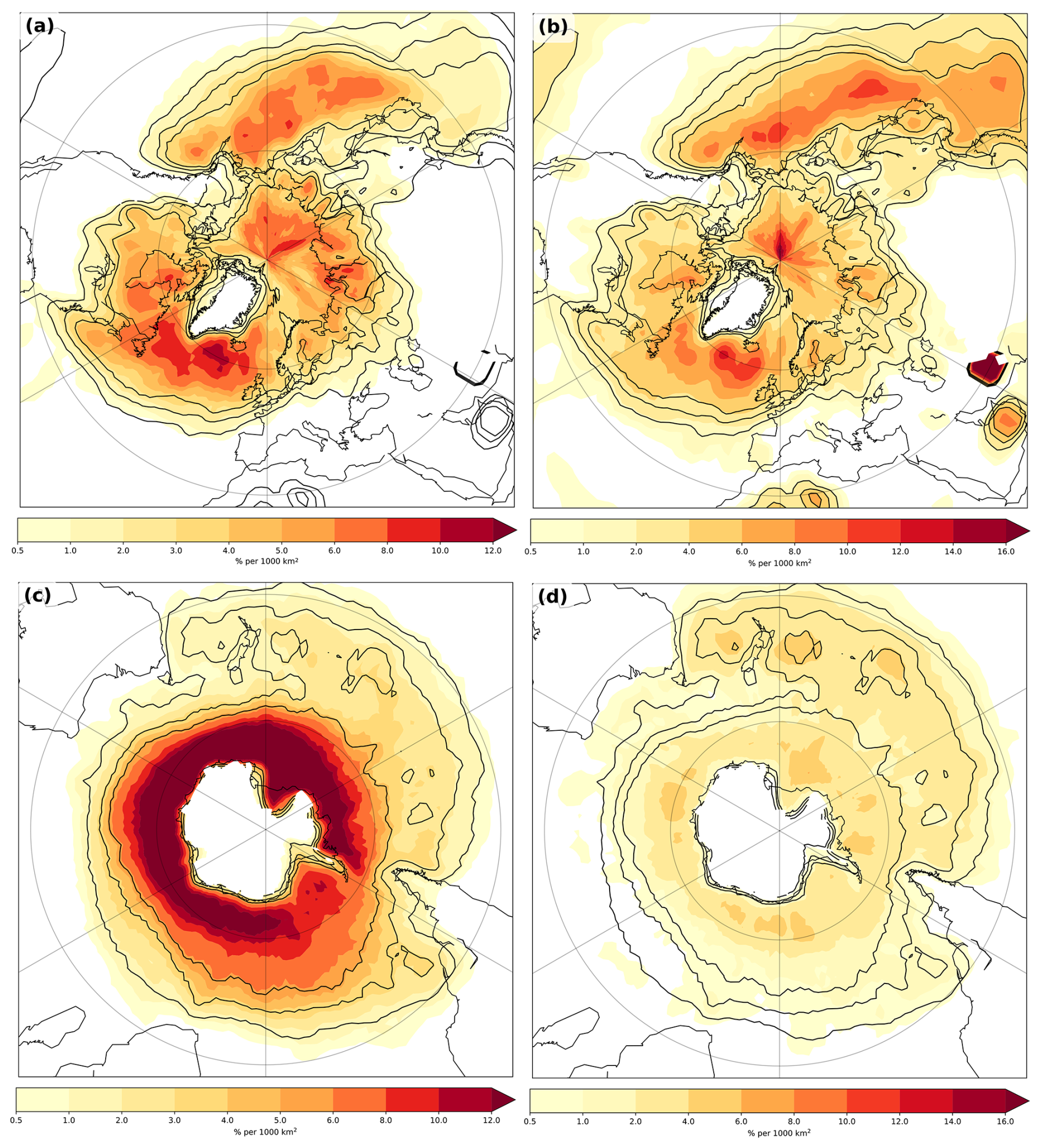
Figure 5 As Fig. 3, but for the respective summer seasons.

4 Characteristics of clustered cyclones

Some studies argue for a systematic mechanism associated with cyclone clustering (Priestley et al., 2017; Weijenborg and Spengler, 2020) and that clustering is generally associated with stronger cyclones (Vitolo et al., 2009). We test these findings by assessing differences in cluster size and storm intensity, both for all clusters as well for the two sub-types of clustering. In this section, we only investigate cyclones during the the respective winter seasons (DJF for the Northern Hemisphere, and JJA for the Southern Hemisphere), as extratropical cyclones have the highest occurrence and intensity during winter.

We define the size of a cluster as the number of cyclones in a cluster and limit out analysis to cyclones in the regions demarcated in Fig. 2b and d. In general, the likelihood of having a cluster of size n decays exponentially (Fig. 6a). This decay is stronger for stagnant clusters. While there are no big differences between the different basins, there are relatively more larger stagnant clusters for the North Atlantic and North Pacific (Fig. 6b–c) compared to the Southern Hemisphere (Fig. 6d–f). In contrast, specifically for the South Atlantic and South Indian Ocean, there are relatively few stagnant clusters (Fig. 6e).

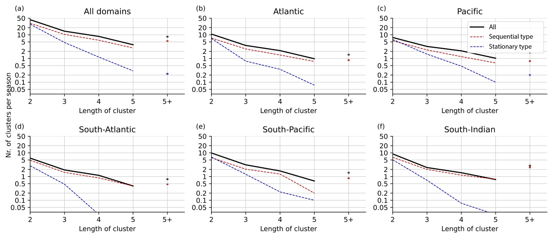
Figure 6 Number of clusters for the respective winter season as function of size of cluster for all clusters (black line), sequential type (red line), and stagnant type (blue line). (a) Top left for all regions. (b–f) For Atlantic, Pacific, South Atlantic, South Pacific, and South Indian Ocean, respectively.

4.1 Cyclone intensity

To investigate if clustered cyclones are stronger, we compare the intensity of the strongest cyclone in our detected clusters with the strongest cyclone in a cluster of same size with randomly assigned cyclones from the same region. We find that clustered cyclones are generally stronger and that solo cyclones are generally weaker (Fig. 7). The qualitative differences between the different basins are small with slightly stronger clustered cyclones in the North Atlantic and North Pacific. The differences in intensity for clustered and non-clustered cyclones is, however, less in the three basins in the Southern Hemisphere. Specifically the South Indian Ocean and South Pacific stand out with only a small difference in intensity. This indicates that clustering might be dynamically different for the storm tracks in the Northern and Southern Hemisphere. Results are similar when using the mean intensity instead of the strongest cyclone in a cluster (see Supplement, Figs. S2 and S3).

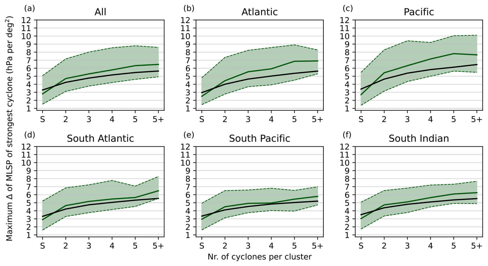
Figure 7 Cyclone intensity as function of size of cluster, i.e. the number of storms in a cluster. The bin denoted with ”S” indicates the strength of solo (non-clustered) cyclones. Green solid line indicates median values and variability between the 10 % and 90 % quantiles is indicated by shading. The black line indicates expected value from randomly chosen clusters.

The strongest cyclones in sequential type clusters are stronger compared to randomly selected cyclones (Fig. 8a). One might have anticipated this result for sequential type clustered cyclones, as they are most likely associated with a stronger jet and baroclinicity. This difference is largest for the North Atlantic and the North Pacific (Fig. 8b–c), while there are only small differences for the South Indian Ocean.

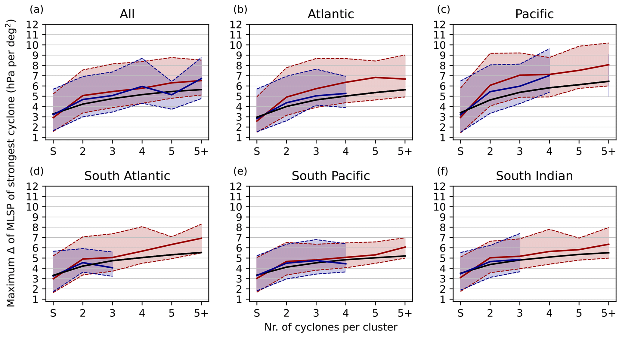
Figure 8 As Fig. 7 but for sequential type (red solid line and shading, for mean and 10 % to 90 % quantiles) and stagnant type (blue shading). Black line indicates expected value from randomly chosen clusters.

In contrast, the median of the strongest cyclones in stagnant clusters of size n falls between that of sequential type clusters and the expected value of a randomly chosen cyclone (Fig. 8a). The 90 % quantile for the stagnant type is also lower as that of the sequential type, with the difference in intensity being larger for the North Pacific compared to the North Atlantic (Fig. 8a and b). For the Southern Hemisphere the intensity of stagnant clustered cyclones and solo cyclones is very similar (Fig. 8d–f). These differences in intensity between the two types of clusters strongly suggest that there are dynamical differences between these two types.

To investigate the local impact of spatio-temporal clustered cyclones, we determine how often a cyclone is present with an intensity higher than the 90 % quantile of the intensity at that particular location. We therefore first determine the 90 % percentile of the Laplacian of the mean sea level pressure at each location and then count how often a cyclone has an intensity exceeding this threshold. We do this analysis for both clustered and non-clustered cyclones. Even though the number of clustered cyclones is lower, the absolute number of intense clustered cyclones is higher than that of intense non-clustered cyclones (Fig. 9a and b). This is especially the case along the storm tracks in the North Atlantic and North Pacific, as well as just north of the United Kingdom and along the coast of Norway. For the exit of the Pacific storm track, this is less clear, with even higher densities of intense non-clustered cyclones along the coast of the United States. However, along the storm track exit regions in both the Atlantic and the Pacific, the intensity of clustered cyclones is shifted towards higher intensities (Fig. 9c).

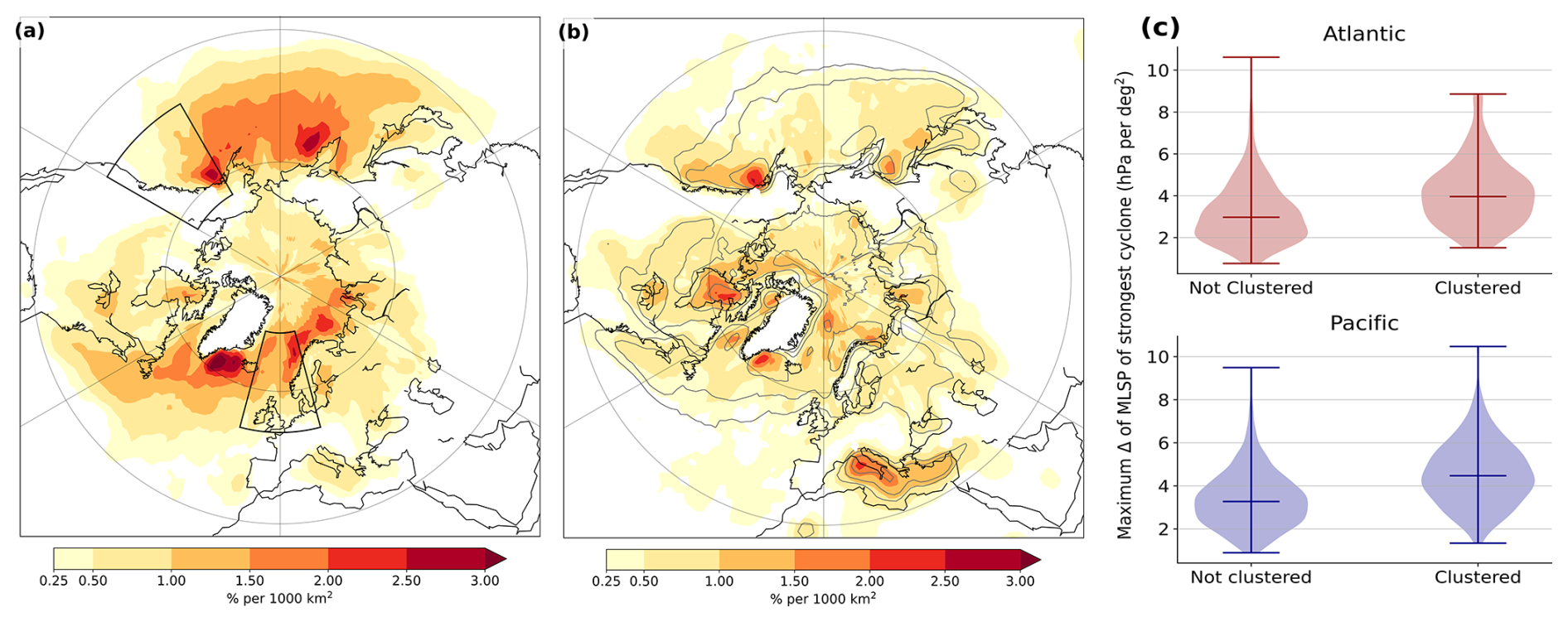
Figure 9 (a) Density of clustered cyclones with an intensity of at least the 90 % quantile at that location during the winter season. (b) as (a), but for non-clustered cyclones. (c) Violin plot of intensity of clustered and non-clustered cyclones at the storm track exit regions indicated by the black boxes in (a).

4.2 Cluster size and cyclone intensity

Given that sequential type clusters are most likely associated with a strong baroclinicity and jet, we investigate the relation between the strength of cyclones and the length of overlap δx_overlap along their tracks in space-time. If a cyclone is connected to multiple cyclones, the maximum overlap δx_overlap is used. This maximum overlap is a measure of how “clustered” a specific cyclone is (see Sect. 2.1 for more details). Solo (non-clustered) cyclones are put in the lowest bins (δx_overlap<1.5 Rossby Radius in Fig. 10a and δt_overlap<2 d in Fig. 10b).

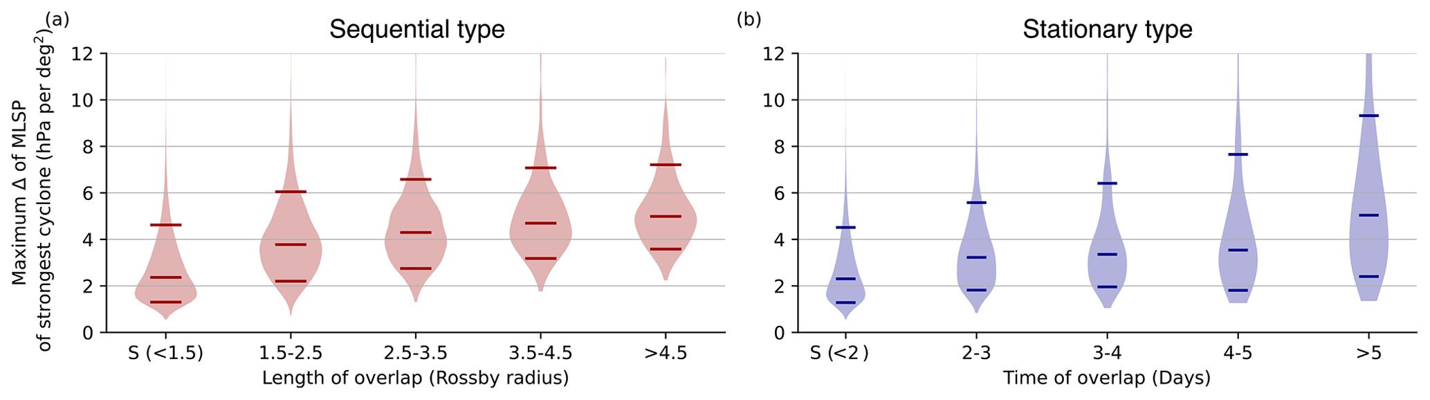
Figure 10 Violin plots for cyclone intensity for (a) sequential type clusters as function of Rossby radius and (b) Stagnant type clusters as function of time overlap. The bin denoted with “S” indicates the intensity of solo (non-clustered) cyclones. The Medians and 10 % and 90 % quantiles in each violin plot are indicated by solid lines.

There is an increase in cyclone intensity, with respect to the length of overlap (Fig. 10a), especially up to about three Rossby radius. Contrary to the sequential type clusters, clustered cyclones of the the stagnant type feature a weaker increase in intensity with increasing cluster size (Fig. 10b). The median for the stagnant type clusters increases up to 50 % compared to solo cyclones, while the median for cyclones of the sequential type clusters increases up to almost twice that compared to solo cyclones. This again indicates that the two types of clusters are dynamically different.

4.3 Cyclone intensity within a cluster

We showed that clustered cyclones are more intense than solo cyclones. To check if there are consistent differences in cyclone intensity within a cluster, we select clusters of at least size n=3 and distinguish between “primary” (first), secondary+, and final cyclones in a cluster.

There are only small intensity differences in intensity within sequential type clusters (Fig. 11a), suggesting the existence of processes that replenish baroclinicity during the clustering period, as suggested by Weijenborg and Spengler (2020). The last cyclone in a sequential type cluster is slightly less intense than the previous cyclones in the cluster. Using the minimum pressure instead of the maximum Laplacian of the mean sea level pressure as an intensity measure yields consistent results (Fig. S4).

In contrast, there is a decrease in cyclone intensity throughout the lifetime of stagnant clusters, with the primary cyclone being the strongest (Fig. 11b). While the primary cyclone is almost as strong as the primary cyclone in sequential type clusters, subsequent cyclones are less intense, with the final cyclone being the weakest. This decrease in intensity is both visible in the median as well as in the 10 % and 90 % quantiles.

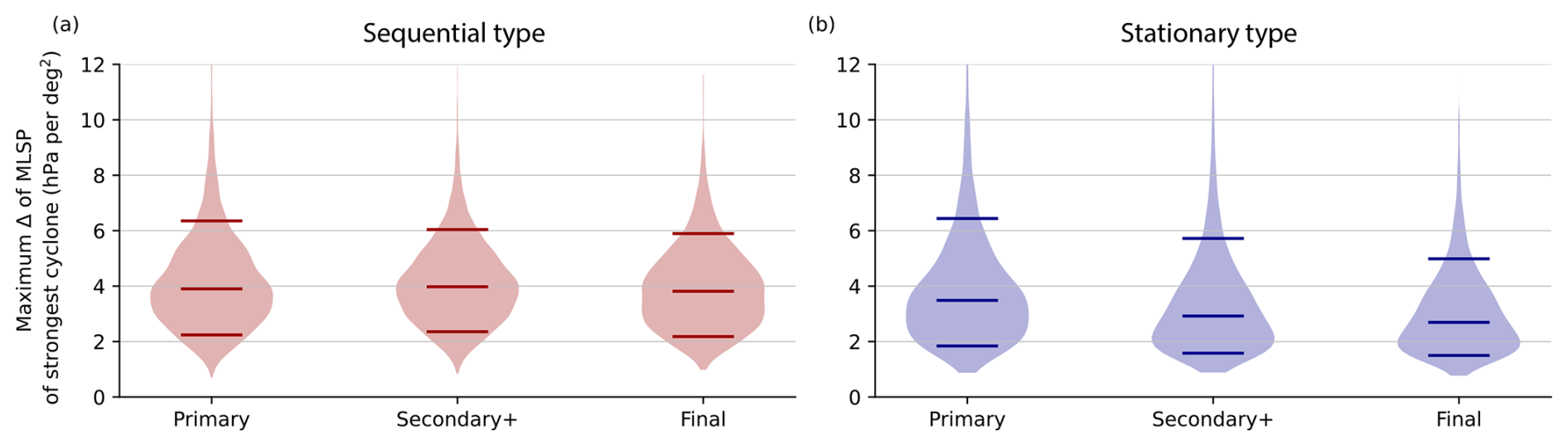
Figure 11 Violin plots for the intensity of cyclones for (a) sequential type and (b) stagnant type for the first (Primary), all secondary, and final cyclones in each cluster. Medians and 10 % and 90 % quantiles are indicated by horizontal lines.

5 Conclusions

We introduce a detection algorithm for spatio-temporal cyclone clustering that can be used globally, where we identify if multiple cyclone tracks are in close proximity in space and time. We subdivide cyclone clusters into two different sub-types, which we refer to as sequential and stagnant types, where cyclones in the former category need to travel over a minimum distance along a similar track, similar to cyclone families (Bjerknes and Solberg, 1922), whereas the latter contains less mobile cyclones occurring in a similar region over a given time.

Using our diagnostic, we find that cyclone clustering mainly occurs near the main storm tracks in the North Atlantic and North Pacific, with the highest fraction of clustered cyclones just to the south of the storm tracks. In the Southern Hemisphere, highest frequencies are found in the South Indian Ocean. In general the sequential-type cluster is found more towards the storm track entrance, while stagnant clusters are more frequent at the storm track exit.

Clustered cyclones are stronger than non-clustered cyclones, with this difference increasing with the number of cyclones in a cluster. This increase in intensity is stronger for sequential type cyclones, for which the intensity of cyclones also increases when the distance that cyclones follow each-other increases, suggesting a replenishment of baroclinicity during the clustering period. In contrast, cyclones from stagnant type clusters are not stronger compared to non-clustered cyclones, suggesting that the mechanisms for the two types clustering are different. There are also some regional differences between the Northern and Southern Hemisphere, with generally stronger clustered cyclones in the Northern Hemisphere.

Our results are consistent with previously published climatologies of cyclone clusters (Priestley et al., 2017, 2020b). As in Priestley et al. (2020b), clustering in the Northern Hemisphere winter mainly follows the storm track, with genesis occurring often at the storm track entrance at the Gulf stream and the Kuroshio regions. However, our results are different to Mailier et al. (2006), who found the highest frequency of clustering at the storm track exit. This difference can be attributed to the statistical nature of their algorithm. While their algorithm focuses on the regularity of cyclone occurrence in a given month, our algorithm determines the absolute number of spatio-temporally clustered cyclones.

Using our global detection and classification, future research can address underlying mechanisms of cyclone clustering and investigate regional differences. Furthermore, due to our sub-categorisation into two different types of cyclone clustering, one can assess dynamical differences in the initiation and evolution of sequential and stagnant type of cyclone clustering. Last but not least, given that our algorithm also distinguishes between primary and secondary cyclones in a cluster, one can further differentiate how cyclones within a cluster influence each other. The latter is of particular interest when considering the mechanism of secondary cyclogenesis and maintenance of baroclinicty during sequential type clusters.