Atmospheric blocking in an aquaplanet and the impact of orography

Many fundamental questions remain about the roles and effects of stationary forcing on atmospheric blocking. As such, this work utilizes an idealized moist general circulation model (GCM) to investigate atmospheric blocking in terms of dynamics, geographical location, and duration. The model is first configured as an aquaplanet, then orography is added in separate integrations. Block-centered composites of wave activity fluxes and height show that blocks in the aquaplanet undergo a realistic dynamical evolution when compared to reanalysis. Blocks in the aquaplanet are also found to have similar life cycles to blocks in model integrations with orography. These results affirm the usefulness of both zonally symmetric and asymmetric idealized model configurations for studying blocking. Adding orography to the model leads to an increase in blocking. This mirrors what is observed when comparing the Northern Hemisphere (NH) and Southern Hemisphere (SH), where the NH contains more orography and thus more blocking. As the prescribed mountain height increases, so do the magnitude and size of climatological stationary waves, resulting in more blocking overall. Increases in blocking, however, are not spatially uniform. Orography is found to induce regions of enhanced block frequency just upstream of mountains, near high pressure anomalies in the stationary waves, which is poleward of climatological minima in upper-level zonal wind, while block frequency minima and jet maxima occur eastward of the wave trough. This result matches what is observed near the Rocky Mountains. Finally, an analysis of block duration suggests blocks generated near stationary wave maxima last slightly longer than blocks that form far from or without orography. Overall, the results of this work help to explain some of the observed similarities and differences in blocking between the NH and SH and emphasize the importance of general circulation features in setting where blocks most frequently occur.

1 Introduction

Atmospheric blocks are quasi-stationary anticyclones that can cause temperature extremes (Sillman et al., 2011; Pfahl and Wernli, 2012), steer hurricanes and extratropical cyclones (Mattingly et al., 2015; Booth et al. 2017a, respectively), and induce persistent weather (Cassou et al., 2005; Dole et al., 2011; Brunner et al., 2018). For readers looking for a comprehensive review of blocking; see Woollings et al. (2018). Despite the expensive and sometimes deadly impacts of blocks, many fundamental questions remain regarding their behavior, and models tend to underpredict blocks in terms of their frequency and duration (D'Andrea et al., 1998; Matsueda et al., 2009). As such, this paper utilizes an idealized general circulation model to expand our understanding of blocks, focusing on the representation in models configured with and without mountains.

Some have argued that blocks are consequences of an interaction between eddies and stationary waves induced by orography (Egger, 1978; Charney and DeVore, 1979; Tung and Lindzen, 1979; Luo, 2005). These studies suggest mountains are critical for the overall existence of blocking and setting the location of climatological block frequency maxima. On the other hand, Shutts (1983) used a barotropic model to show that blocking flows do not necessarily need stationary forcing and can arise purely through interactions between transient eddies. Confirming this, Hu et al. (2008), Hassanzadeh et al. (2014), and Nabizadeh et al. (2019) have more recently shown that blocks do indeed occur in idealized models in the absence of zonally asymmetric forcing.

This suggests the extratropical cyclones (i.e., synoptic-scale eddies) that occur upstream of the blocking regions may be key. Colucci (1985) and Pfahl et al. (2015) show that extratropical cyclones can impact blocks downstream of the storm track exit region. In a related theory, blocks are linked to Rossby wave-breaking (Pelly and Hoskins, 2003; Berrisford et al., 2007; Masato et al., 2012), which primarily occurs in regions of weak westerly flow.

Hu et al. (2008) presents case studies that show blocks in an aquaplanet model behave in a realistic manner. They also find that blocks in their aquaplanet model occur more frequently than what is observed in nature, regardless of hemisphere, which is contradictory to the idea that stationary waves facilitate blocking episodes. The results of Hu et al. (2008), however, are complicated by known discrepancies within the community regarding the identification (e.g., Barnes et al., 2012) and seasonality (Barriopedro et al., 2010) of blocking. In Hu et al. (2008), results from their perpetual equinox aquaplanet are compared to Wiedenmann et al. (2002), who use a different block identification algorithm on reanalysis over all seasons. Thus, questions remain regarding the relative frequency of blocks with and without the presence of mountains.

The climatological spatial distribution of blocks is well documented. In the cool months of the Northern Hemisphere (NH), two main regions of blocking occur at the northeastern edges of the Atlantic and Pacific Ocean basins (Barriopedro et al., 2006; Croci-Maspoli et al., 2007; Dunn-Sigouin and Son, 2013). In the Southern Hemisphere (SH), one main region of blocking exists, located southwest of South America (Renwick, 2005; Parsons et al., 2016; Brunner and Steiner, 2017). Overall, blocking occurs more frequently in the Northern Hemisphere than the Southern Hemisphere. This difference in blocking frequency is assumed to related to the stronger stationary wave in the NH (Nakamura and Huang, 2018), often attributed to more prominent midlatitude topography and land–sea contrasts, e.g., Held et al. (2002). However, to our knowledge, no study has confirmed this assumption.

Previous work suggests that the spatial distribution of blocking frequency (hereafter, the blocking climatology) is dependent on the behavior of the stationary waves, jet streams, and storm tracks. Nakamura and Huang (2018), for example, propose that blocking is most ubiquitous in regions where the positive anomaly in the stationary wave maximizes and mean westerly flow is weak. Work by others on the effects of transient eddy forcing on blocks (Shutts, 1983; Nakamura et al., 1997; Takaya and Nakamura, 2001; Wang and Kuang, 2019) shows the importance of the storm tracks. The work presented here aims to better characterize the manner in which the spatial distribution of the stationary waves, jet streams, and storm tracks are linked to the blocking climatology.

This article focuses on four main research questions.

1. Are blocks in an aquaplanet dynamically similar to blocks in orographically forced simulations and reanalysis?

2. Does the presence of orography affect the hemispherically averaged frequency of blocking?

3. How does orography affect the spatial distribution of blocking frequency?

4. Does orography affect the duration of blocking events?

To address question 1, we use compositing analysis to compare the life cycles of blocks for an aquaplanet, reanalysis, and a model with orography. For questions 2 and 3, we compare the climatology of blocking, stationary waves, jet streams, and storm tracks for models with different orographic configurations. To answer question 4, we carry out an analysis that examines the sensitivity of block duration to mountains.

2 Methods

2.1 Reanalysis data

Although the focus of this paper is on idealized numerical modeling experiments, we also present results using reanalysis to motivate our work. The reanalysis used is the ECMWF ERA-Interim dataset (Dee et al., 2011). ERA-Interim (ERAI) has been shown to represent winter midlatitude storms as well as, and in some cases better than, other reanalyses (Hodges et al., 2011). Therefore, it likely does a reasonable job at capturing atmospheric blocking. ERA-Interim is produced using a model with roughly 0.67^∘ resolution, but it is available to download at different resolutions. Herein, we used data with a 1.5^∘×1.5^∘ horizontal resolution. For this analysis we focus only on the cool season from 1979-2017, which is defined as November–March and May–September for the Northern Hemisphere and Southern Hemisphere, respectively. Blocks are most abundant during these months (Tibaldi et al., 1994; Barriopedro et al., 2010).

2.2 Idealized model configuration

This work utilizes an idealized moist GCM described by Clark et al. (2018, 2019), which is modified from that introduced by Frierson et al. (2006, 2007) and later altered by Frierson (2007) and O'Gorman and Schneider (2008). The model is configured to use 30 unevenly spaced vertical sigma coordinate levels and T₄₂ spectral resolution, corresponding to 64 latitude by 128 longitude grid points when transformed to a latitude–longitude grid. Earth-like orbital parameters are used to simulate a full seasonal cycle in solar insolation. The model includes full radiative transfer and simplified physics parameterizations of convection (Frierson, 2007), boundary layer turbulence (Troen and Mahrt, 1986), and surface fluxes. There is no treatment of cloud radiative effects or condensed water in the atmosphere.

An aquaplanet configuration is run as the control integration. For the integrations with mountains, configurations of topographical forcing are simulated by modifying the model surface height and using a simplified treatment of land following Geen et al. (2018) and Vallis et al. (2018). Like Cook and Held (1992) and following Lutsko and Held (2016), perturbations to the surface height are introduced in the form of Gaussian mountains centered at 45^∘ N with half-widths of 15^∘ in both the latitude and longitude dimensions. Several configurations are examined in this work.

• a.

  Aquaplanet: idealized model with no orography;

• b.

  SingleMtn: four separate integrations with a single Gaussian mountain centered at 45^∘ N, 90^∘ E of variable peak height (1, 2, 3, and 4 km);

• c.

  TwoMtn: one integration with two asymmetrically placed 3 km high Gaussian mountains centered at 45^∘ N, 90^∘ E and 45^∘ N, 150^∘ W, respectively. This placement is to loosely mimic the wide (Pacific) and short (Atlantic) zonal extents of the NH ocean basins.

The 3 km SingleMtn and TwoMtn configurations are shown in Fig. 1. Ocean grid cells are represented using a slab ocean with a depth of 20 m. For simplicity we prescribe uniformly zero Q flux, meaning that we assume that in the time mean, the net flux of energy from the ocean to the atmosphere is zero at all surface grid cells. In the configurations with mountains, land grid cells are defined as locations where the height is greater than 1∕100th of the maximum surface height (3 km), corresponding to a height threshold of 30 m. As in Geen et al. (2018) and Vallis et al. (2018), land is simulated by reducing the slab ocean depth to 2 m (effectively reducing the heat capacity) and limiting evaporation using a bucket hydrology model. A uniform surface albedo of 0.26 is used to obtain a global annual mean surface temperature resembling that of the Earth. Each configuration is integrated for 40 years, but the first 10 years are discarded as spin-up time. Thus, the results presented here are for years 11–40 of each integration. The 6-hourly data sets are used for the analyses in this paper, and the results are presented for the Northern Hemisphere cool season, defined as the 5 months centered on the minimum in solar insolation. The model data are interpolated to the 1.5^∘×1.5^∘ horizontal ERA-Interim resolution prior to any analysis.

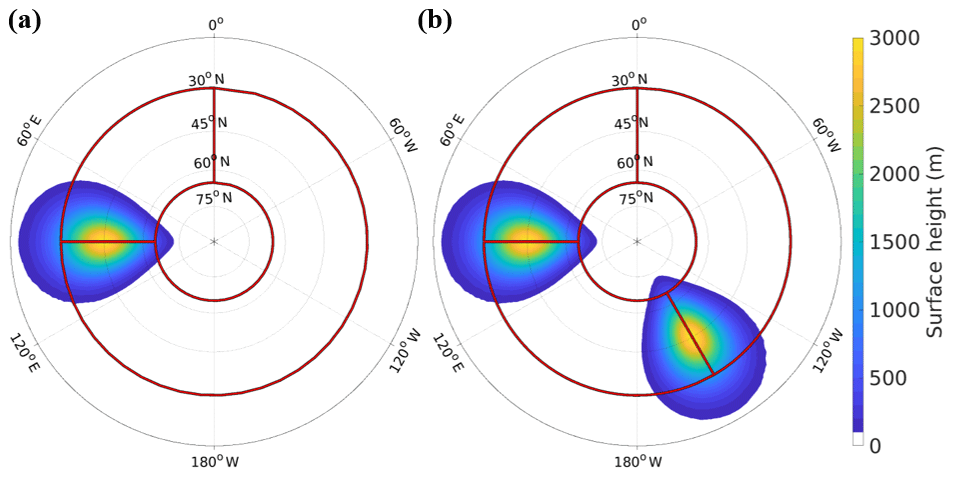
Figure 1 Surface height (shading) of the idealized model integrations with (a) a single 3 km high Gaussian mountain centered at 45^∘ N, 90^∘ E and (b) two 3 km high Gaussian mountains centered at 45^∘ N, 90^∘ E and 45^∘ N, 150^∘ W, respectively. The red outlines indicate the block genesis regions described in Table 1.

2.3 Block detection and tracking

Here we use a 500 hPa geopotential height (Z₅₀₀) hybrid metric that utilizes the Z₅₀₀ anomaly and meridional gradient. This metric was chosen for its robustness in terms of capturing high-amplitude events involving wave-breaking (Dunn-Sigouin and Son, 2013) and because it only requires the Z₅₀₀ field, which simplifies tracking when analyzing large datasets. Barnes et al. (2012) finds that utilizing a Z₅₀₀ metric produces similar blocking durations and climatologies to both potential vorticity and potential temperature based metrics. Blocks are detected and tracked using the algorithm described by Dunn-Sigouin and Son (2013), hereinafter referred to as DS13, which is an adaptation of previous methods by Barriopedro et al. (2010) and Sausen et al. (1995). This algorithm searches for large, contiguous regions of persistent, high-amplitude, positive anomalies in the Z₅₀₀ field. Within these regions, Z₅₀₀ must satisfy a meridional gradient reversal condition. What follows is an overview of the block identification algorithm, but specific details can be found in DS13.

1. Z₅₀₀ anomaly calculation: for each grid point poleward of 30^∘ N, from the raw Z₅₀₀ field subtract the running annual mean and mean seasonal cycle as computed in DS13.

2. Normalization of each anomaly value by the sin of its latitude divided by sin of 45^∘: $\frac{\sin \left({\mathit{\varphi }}_{ij}\right)}{\sin \left(\mathrm{45}{}^{\circ }\right)}$, where ϕ_ij is the latitude of an arbitrary grid point with longitude i and latitude j. This normalized anomaly will be referred to as $Z_{\mathrm{500}}^{\prime }$.

3. Calculation of the standard deviation, SD, of all $Z_{\mathrm{500}}^{\prime }$ values: for each month, in a 3-month window centered on a given month.

4. Amplitude threshold: identify contiguous regions of positive $Z_{\mathrm{500}}^{\prime }$, greater than or equal to 1.5^∘ S.

5. Size threshold: regions must be at least 2.5×10⁶ km² in area.

6. Gradient reversal: the meridional gradient of the Z₅₀₀ field within candidate regions must undergo a reversal in sign, as described by DS13.

7. Quasi-stationary condition: for each time step, regions must have a 50 % area overlap with its previous time step (modified from DS13's 2 d overlap, which was applied to daily mean data).

8. Duration condition: blocks must meet the above criteria for at least 5 d (i.e., 20 total 6-hourly time steps).

In case studies using ERAI and the idealized configurations described here, it was observed that two existing blocks sometimes merged with one another to form a single, larger block. We objectively identified this merging process based on extreme shifts in the location of the block centroid (defined as the grid point that is the centroid of the anomalous area associated with the block). If the centroid shifted by more than 1500 km from one 6-hourly snapshot to the next, we labeled the block as a merged event. These merged events represented 23 %–27 % of the total initial blocks found in the idealized model integrations. We judge these events to be unique in terms of their relationship between block duration. Furthermore, the merger blocks create uncertainty in terms of defining a block center for the sake of our block-centered composite analysis. Therefore, we have excluded the merged events from our block-centered compositing and block duration analyses. The blocking climatological analysis, on the other hand, retains all blocks since the primary focus is on the spatial distribution of block frequency, not the individual blocks themselves.

2.4 Analysis metrics

The metrics used to characterize climatological features and blocking in the idealized model data and reanalysis are outlined below.

2.4.1 Stationary wave and Eulerian storm track

The cool-season stationary wave at each point is defined as the anomaly with respect to the zonal mean of the cool-season climatology for the 250 hPa geopotential height field: ${\stackrel{\mathrm{‾}}{Z}}^{*}=\stackrel{\mathrm{‾}}{Z}-\left[\stackrel{\mathrm{‾}}{Z}\right]$, where brackets indicate the zonal mean and the overbar indicates the time mean over cool-season days for all years. This is computed separately for each grid point.

The Eulerian storm track is presented as the standard deviation of a 24 h difference of the daily mean Z₅₀₀ field during the cool season (Wallace et al., 1988; Guo et al., 2009; Booth et al., 2017b). Consider Z₅₀₀(t) to be the daily mean Z₅₀₀ value for an arbitrary grid point. To obtain the storm track:

1. The 24 h difference, $Z_{\mathrm{500}}^{\mathit{\tau }}$, at each grid point is taken as

   $$\begin{array}{}\text{(1)}& Z_{\mathrm{500}}^{\mathit{\tau }}=Z_{\mathrm{500}}(t+\mathrm{1})-Z_{\mathrm{500}}\left(t\right).\end{array}$$

2. Then the standard deviation of $Z_{\mathrm{500}}^{\mathit{\tau }}$ for all cool-season time steps at each grid point is taken to obtain the cool-season Eulerian storm track value at that point.

This is computed separately for each grid point.

2.4.2 Blocking and zonal wind climatologies

The spatial distributions of blocking frequency, referred to hereinafter as the blocking climatologies, are calculated by averaging the block identification flag (1 or 0 respectively) per grid point over all cool-season days. Thus, the blocking climatologies show the percent of cool-season time steps that a block (as defined here) is present. This is computed separately at each grid point.

The 250 hPa zonal wind climatology, hereinafter referred to as $\stackrel{\mathrm{‾}}{U_{\mathrm{250}}}$, is presented as the time mean of the 250 hPa zonal wind over the cool-season months at each grid point.

2.4.3 Wave activity flux vectors

To better characterize the dynamical evolution of blocks within each model, wave activity flux vectors (hereinafter, W) are calculated as described by Takaya and Nakamura (2001), hereinafter TN01. The wave activity flux relates eddy feedback onto the mean state and is essentially the pseudo-momentum associated with Rossby waves. Convergence of W is associated with blocking and an overall slowing or reversal of westerly flow. The formulation of W in TN01 includes a stationary term that dominates for quasi-stationary, low-frequency eddies (i.e., 8 to 30 d timescales), and a non-stationary, group-velocity-dependent term that is more relevant for higher-frequency eddies. Here we calculate only the stationary, horizontal component of W and focus on contributions solely from the low-frequency eddies.

Block-centered composites (as described in Sect. 2.5.1. of this paper) are computed using W for each block during various stages of the block's life cycle. The horizontal components of W are calculated as in TN01. For this, eddy fields are computed with an 8 to 30 d bandpass filter. This is what is described as low-frequency eddies in TN01 and Nakamura et al. (1997). W are given by

$$\begin{array}{}\text{(2)}& \mathit{W}={\displaystyle \frac{p\cos \mathit{\varphi }}{\mathrm{2}\mathrm{|}\mathit{U}\mathrm{|}}}\left(\begin{array}{l}U\left({v^{\prime }}^{\mathrm{2}}-\frac{{\mathrm{\Phi }}^{\prime }}{f}\frac{\partial v^{\prime }}{\partial x}\right)+V\left(-u^{\prime }{v}^{\prime }+\frac{{\mathrm{\Phi }}^{\prime }}{f}\frac{\partial u^{\prime }}{\partial x}\right)\\ U\left(-u^{\prime }{v}^{\prime }+\frac{{\mathrm{\Phi }}^{\prime }}{f}\frac{\partial v^{\prime }}{\partial y}\right)+V\left({u^{\prime }}^{\mathrm{2}}+\frac{{\mathrm{\Phi }}^{\prime }}{f}\frac{\partial u^{\prime }}{\partial y}\right)\end{array}\right).\end{array}$$

This calculation is performed on variables on the 250 hPa pressure surface. For each point p is the pressure and ϕ is latitude. U is the 30 d low-pass filtered horizontal wind vector with zonal and meridional components U and V, respectively. The anomalous zonal wind, meridional wind, and geopotential are given by u^′, v^′ and Φ^′, respectively. Derivatives are computed using finite differencing, where zonal derivatives are weighted by latitude. W is given in m² s⁻².

2.5 Analysis methods

2.5.1 Block-centered compositing

The $Z_{\mathrm{500}}^{\prime }$, W, and ∇⋅W fields are composited around the centroid of each block for the first, strongest, and final days of each block life cycle. To account for the convergence of meridians, relevant fields are projected onto equal-area grids before compositing. The initial time step of a block is the first time step that the block satisfies the amplitude, size, and reversal conditions. The strongest time step of a block is defined as the time step with the greatest $Z_{\mathrm{500}}^{\prime }$ (at a single latitude–longitude location) within a block. The final time step is the last time step that a block satisfies the amplitude, size, and reversal conditions.

The composites presented in this paper only include midlatitude blocks whose centroid are always south of 65^∘ N. This is because we find that the high-latitude blocks exhibit distinct physical behavior. From reanalysis data, high-latitude blocks in the Southern Hemisphere have different dynamical evolution and different impacts on the surrounding flow, as compared to midlatitude blocks (Berrisford et al., 2007). The 65^∘ N cutoff was chosen after estimates showed this to be near the minimum in the meridional potential vorticity gradient, and thus the northern limit of the midlatitude waveguide (e.g., Wirth et al., 2018). Compositing results were robust to changes in cutoff latitude of ±7.5^∘.

2.5.2 Separating blocks by region

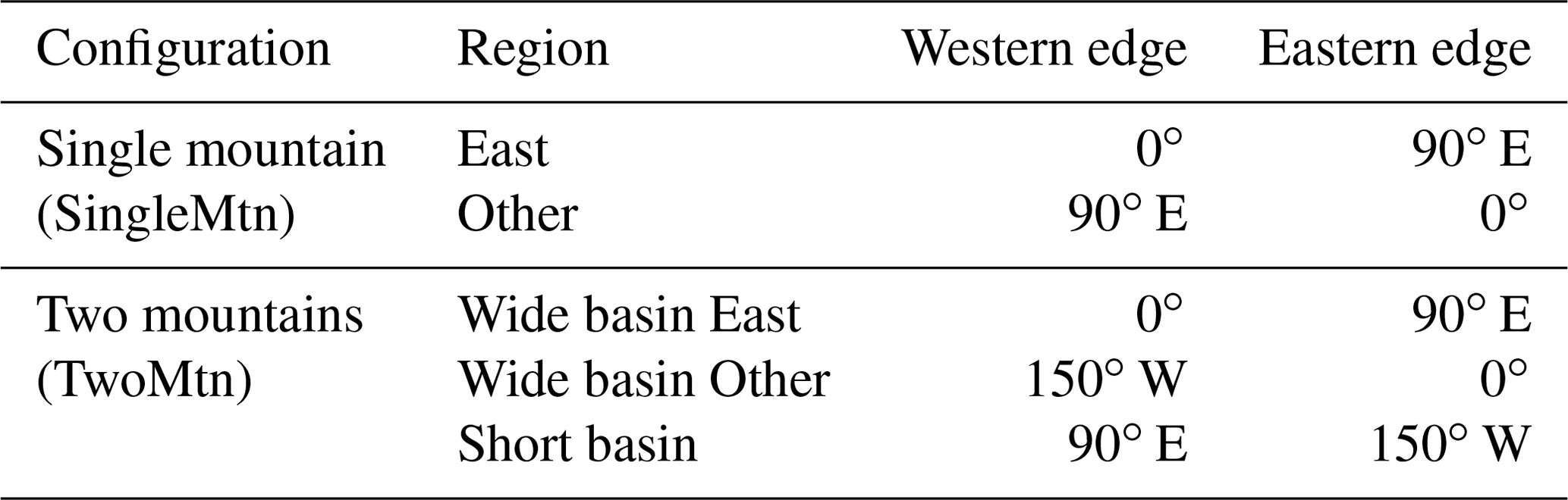
To compare the dynamical evolution of blocks originating near the eastern edge of the ocean basins (denoted as “East”, near the windward side of mountains and the high-pressure maxima of stationary waves) against blocks originating elsewhere (denoted as “Other”), blocks are sorted by their centroid location during their first time step. These regions are outlined in Table 1 and shown in Fig. 1. The East region spans 30–65^∘ N for 90^∘ of longitude upstream, inclusive of the mountain center. For the TwoMtn configuration, “East” and “Other” refer to two regions within the zonally larger ocean basin (which we refer to as the “wide basin”), whereas blocks originating within the zonally smaller ocean basin are denoted as being from the “short basin”.

Table 1 Regions used for subsetting blocks in the compositing and duration analysis. Each region spans 30–65^∘ N, for the longitudes listed in the table.

2.5.3 Block duration probability density distributions

Block duration is defined as the time interval from the initial identification time step to the end of that block's existence – based on the block identification algorithm (described in Sect. 2.3). Each block is thus assigned one duration value. The steps taken to obtain block duration probability density distributions are as follows.

1. Sort blocks into subsets by model configuration and/or basin.

2. Allowing replacement, randomly select a set of block durations within a given subset. The size of the random set is given by the number of blocks in the subset being analyzed.

3. Place the durations yielded by step 2 into n equal-sized bins (n=8 for figures in this paper) ranging from the minimum to maximum duration of cool-season blocks between all model configurations.

4. Steps 2 and 3 are then repeated m times (m=1000 for figures in this paper) to produce an ensemble of m probability density distributions for each subset.

5. For a given subset, the mean probability density distribution is computed by taking the mean of that subset's distributions. This is then smoothed using a running mean.

6. For a given subset, the standard deviation of probability density distribution is computed by taking the standard deviation of that subset's distributions.

The results of this paper are nearly constant with respect to changes in the values of n(±2) and m(±200). For all configurations, distributions and mean values presented for duration exclude any high-latitude blocking (blocks whose centroid are ever poleward of 65^∘ N); 65^∘ N was found to be the most appropriate cutoff in each configuration for the same reasons as described for the aquaplanet compositing.

2.5.4 Statistical significance

For a given grid point and cool season, a block frequency value is computed by averaging all the block identification flag values (1 or 0) for each time step of that cool season. This is done at every grid point for every cool season to yield a 3D matrix of dimensions latitude by longitude by number of years. For each grid point, the distributions of blocking frequency were found to approximately follow Poisson distributions (not shown). Mann–Whitney u tests are implemented for corresponding grid points between a given orographic configuration and a 250-year aquaplanet integration. One strength of the u test is that it does not rely on parametric fitting to any specific distribution. We therefore find this test to be more appropriate than other tests like the t test, which requires fitting to a normal distribution. A 250-year aquaplanet integration is used because the blocking climatology is more zonally symmetric when compared to climatology calculations that use less years. This is done to identify regions of enhanced and suppressed blocking frequency in the topographic integrations.

Significance testing for hemispherically averaged block frequency statistics are done by calculating area-averaged blocking frequency for each cool season. For each configuration, this yields a one-dimensional array of values with a length that matches the number of years in the simulation. A two-sample Welch's t test is then used to examine significant differences in hemispherically averaged block frequency between idealized model configurations. We find this t test to be appropriate for this analysis because it accounts for the variances of both samples, and distributions of hemispherically averaged blocking frequency were found to be normally distributed (not shown).

Significance testing for mean block duration also utilizes a u test to compare differences between the various configurations and regions. A 95 % confidence interval is imposed as the significance threshold for all significance testing.

3 Results

3.1 Blocking in the aquaplanet, dynamical aspects, and intermodel comparison

On average, 12.9 blocks per cool season are identified for each hemisphere of the aquaplanet. The presence of blocking in this model configuration is consistent with previous studies that also find blocking in GCM's with zonally symmetric forcing (Hu et al., 2008; Hassanzadeh et al., 2014; Nabizadeh et al., 2019). Figure 2 shows a snapshot of the first day of an arbitrary block in the aquaplanet. Upstream and coincident with the block, a Rossby wave pattern can be observed in both the Z₅₀₀ and $Z_{\mathrm{500}}^{\prime }$ fields (Fig. 2 – the Z₅₀₀ contours show a wave-like feature, and the $Z_{\mathrm{500}}^{\prime }$ field shows an alternating pattern of low and high anomalies in the zonal direction). The presence of these features during the formation of a block agrees with previous work for both simplified (Berggren et al., 1949; Rex, 1950; Colucci, 1985; Nakamura et al., 1997; Hu et al., 2008), and comprehensive models (TN01; Yamazaki and Itoh, 2013; Nakamura and Huang, 2018; Dong et al., 2018).

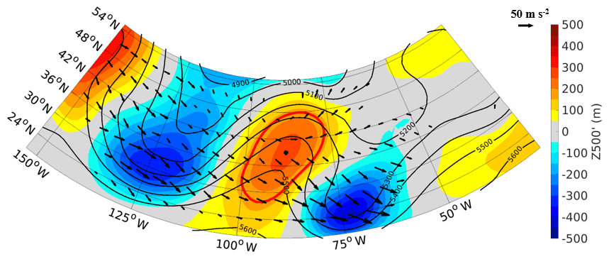
Figure 2 The 500 hPa geopotential height (black contours), 500 hPa geopotential height anomaly (shading), outline of blocked area (red contour), and wave activity flux vectors W (black arrows), for the first day of a blocking episode in the aquaplanet run. The black dot inside the block denotes the block centroid. Geopotential height contours are in 100 m intervals. W with magnitudes less than 20 m² s⁻² are removed.

In Fig. 2 near 75–85^∘ W, a characteristic overturning of the Z₅₀₀ contours indicative of anticyclonic Rossby wave breaking (Masato et al., 2012; Davini et al., 2012) is also observed. Concentrated, large magnitude W are found just upstream of, and propagating into, the block, and a relative absence of large magnitude W occurs downstream of the block. On the downstream equatorward flank of the block, converging W consistent with a slowing of the zonal mean flow is observed. The behavior of W during the genesis of this block case study agrees with Nakamura et al. (1997) and TN01 and is consistent with Nakamura and Huang's (2018) description of blocking as a traffic jam of wave activity fluxes.

Block-centered compositing analysis is used to confirm that, on average, the blocks identified in the aquaplanet model evolve in a dynamically similar manner to models with zonally asymmetric forcing. Figure 3 shows block-centered composites of $Z_{\mathrm{500}}^{\prime }$, W, and ∇⋅W for blocks over the NH oceans and for the SH as well (Fig. 3, rows 1 and 2, respectively). In both panels only blocks anchored in the midlatitudes are considered (i.e., occurring between 30 and 65^∘ in latitude). For the sake of comparison with the aquaplanet, blocks over land are excluded. For the idealized model, we show blocks from the aquaplanet (Fig. 3, row 3) and the East region (see Table 1 and Fig. 1) of the 3 km single-mountain configuration (3 km SingleMtn East, Fig. 3, row 4). The East region of the 3 km SingleMtn was chosen to isolate blocks generated in the model that form near the high-pressure anomaly of stationary waves. However, block-centered composites for all orographic configurations (i.e., 1, 2, 3 km, and TwoMtn), and each of their respective regions yielded similar results (not shown), with little to no regional variation – this result is discussed again below.

Figure 3 For cool-season blocking events, block-centered composites of positive 500 hPa geopotential height anomalies (solid contours), negative 500 hPa geopotential height anomalies (dotted contours), W (arrows), and ∇⋅W (shading). (a, e, i) Computed with NH blocks over ocean in ERA-Interim. (b, f, j) Computed with SH blocks in ERA-Interim. (c, g, k) Computed with blocks in the aquaplanet integration. (d, h, l) Computed with blocks in the 3 km single-mountain integration. The left, middle, and right columns are composites over the first, strongest, and last time steps of blocking episodes, respectively. Positive (negative) 500 hPa geopotential height anomaly contours are in 50 m (−10 m) intervals with outer contour 50 m (−30 m); magnitudes less than 20 m² s⁻² are removed. Latitude and longitude are defined relative to the composite block center.

The onset of blocking in the composites (Fig. 3, column 1) is qualitatively similar to that found in the case study (Fig. 2). The Z₅₀₀ anomalies all show a positive anomaly at the center of the composite and negative anomalies upstream. In the NH, this upstream anomaly has two closed centers (Fig. 3a), whereas the SH and the idealized configurations each have only one. We have subset the NH observations for the North Atlantic and North Pacific (not shown), and this difference is mainly due to the blocks in the North Atlantic.

The reanalysis and idealized model results all show W convergence (i.e., blue shading) on the downstream-equatorward flanks of composite blocks during onset (shading in Fig. 3, column 1). The W convergence is stronger in the SH and the aquaplanet (Fig. 3b and c) when compared to the NH, and the idealized configurations that include orography (Fig. 3a and d). W (vectors in Fig. 3) are weaker in the NH at onset (Fig. 3a) as compared to the SH and the idealized model. This difference is mainly attributable to the blocks in the North Pacific (not shown) and is likely due to the fact that the W shown are for low-frequency eddies only. As discussed in Nakamura et al. (1997), in the North Pacific contributions from low-frequency eddies plays a lesser relative role as compared to the North Atlantic.

For composites over blocks at maximum strength (Fig. 3, middle column), the positive Z₅₀₀ anomaly has strengthened, and a similar pattern of ∇⋅W is observed between the reanalysis and the models. Convergence of W on the downstream equatorward flank of the composite blocks are enhanced compared to onset, and the envelope of greatest W is now within the high-pressure center. Upstream, downstream, and equatorward low-pressure centers are also evident when the composite blocks are at peak strength, though the pattern is not as clean in idealized model composites (Fig. 3g and h) compared to reanalysis (Fig. 3e and f).

On the final day of the block life cycles (Fig. 3, third column), each respective composite block's Z₅₀₀ anomaly weakens, and low pressure is concentrated downstream from the block. Weak values of W exit the block downstream of the high-pressure maximum during this time (Fig. 3j, k, and i). A net divergence of W from the blocked region is indicative of a return to westerly zonal flow as the block dies out. The buildup of W upstream and inside the composite block during amplification and the release of W downstream during decay are consistent with downstream development, as described in Danielson et al. (2006).

Block-centered composites for the aquaplanet are qualitatively similar to composites for reanalysis, and the similarities are strongest between SH and aquaplanet (Fig. 3). This is consistent with the fact that the SH has less orography than the NH. However, we remind the reader that surface forcing in the SH is still asymmetric, as discussed in Berrisford et al. (2007). Overall, however, the similarities for the model and reanalysis, regardless of orography, show the potential utility of an aquaplanet model for understanding the fundamental physics of blocking. Similarities between blocks in the aquaplanet and the orographic configurations show that blocks behave in a similar manner with or without mountains as a source of zonally asymmetric forcing.

On the other hand, the differences between the NH and SH in observations are greater than the differences between the aquaplanet and the blocks in the model configured with mountains (and this result is true even if we use all blocks in the 3 km single-mountain model rather than just those near the anticyclonic anomaly of the stationary wave). Thus, the model is missing some details of the internal dynamics of the blocks, as it related to the presence of orography. With this in mind, we now shift our focus to the climatological flow features and blocking climatology.

3.2 Climatological analysis

The majority of theories on blocking formation and maintenance (summarized in the review by Woollings et al., 2018) imply that stationary waves, storm tracks, and upper-level mean flow all might play important roles setting the spatial distribution of blocking frequency. These quantities are now examined for the aquaplanet, reanalysis, and model integrations with mountains. In our discussion of the climatological features in reanalysis and the SingleMtn configurations, we have chosen the following approach: we first discuss the stationary wave because it is the most fundamental metric that changes when adding mountains; following this, we discuss blocking and its relationship to the jet stream. We close the analysis with a discussion of the storm tracks. This choice of the order is motivated by recent theory from Nakamura and Huang (2018) that put greater emphasis on the influence of the jet stream and stationary waves on blocking.

3.2.1 The aquaplanet

For the aquaplanet, the stationary wave, storm track, and $\stackrel{\mathrm{‾}}{U_{\mathrm{250}}}$ are zonally symmetric (Fig. 4a and b). However, the blocking climatology is not zonally symmetric after 30 years (Fig. 4b). We find that it takes 250 years for the aquaplanet blocking climatology to approach zonal symmetry (Fig. 4c and d). However, for the models with orography, the time to reach convergence is likely not as large. We deduced this from the following analysis: we generate 20-year climatologies using randomly sampled years from our 30-year integrations and compare them. For the configurations with orography, the blocking climatology is spatially consistent, whereas for the aquaplanet each climatology has a unique spatial distribution (not shown). Therefore, we believe that 30 years of model runs provides a usable level of convergence of the spatial climatology of blocking in the integrations with mountains.

Figure 4 (a, b) For 30 cool seasons (November–March) in the aquaplanet, (a) the stationary wave (shading) and storm track (heavy black contours), and (b) the blocking climatology (shading) and $\stackrel{\mathrm{‾}}{U_{\mathrm{250}}}$ (heavy black contours) for the idealized model aquaplanet integration. (c, d) Blocking climatology (shading) for (c) 100 and (d) 250 cool seasons in the aquaplanet. In (a) storm track contours are in 10 m intervals where the outer contour is 50 m. In (b) $\stackrel{\mathrm{‾}}{U_{\mathrm{250}}}$ contours are in 5 m s⁻¹ intervals where the outer contour is 30 m s⁻¹.

3.2.2 Reanalysis

The different orographic configurations of the Northern Hemisphere and Southern Hemisphere produce distinct spatial distributions of general circulation features and atmospheric blocking (Fig. 5). Stationary wave patterns can emerge due to land–sea heating contrasts, drag, and flow deflection by topography (e.g., Held et al., 2002). The two strongest regions of anomalous high-pressure in the NH are located on the windward side of the Rocky Mountains and near the western edge of Europe (Fig. 5a). In the SH, the high-pressure maximum is southwest of South America and a secondary maximum can be found southeast of Australia (Fig. 5b). These results are consistent with previous work (Valdes and Hoskins, 1991; Quintanar and Mechoso, 1995; Held et al., 2002; White et al., 2017).

Figure 5 (a, b) Cool-season stationary wave (shading) and storm track (heavy black contours) for the (a) Northern Hemisphere and (b) Southern Hemisphere in ERA-Interim. Storm track contours are in 10 m intervals where the outer contour is 50 m. (c, d) Cool-season blocking climatology (shading) and $\stackrel{\mathrm{‾}}{U_{\mathrm{250}}}$ (heavy black contours) for the (c) Northern Hemisphere and (d) Southern Hemisphere in ERA-Interim. $\stackrel{\mathrm{‾}}{U_{\mathrm{250}}}$ contours are in 5 m s⁻¹ intervals where the outer contour is 10 m s⁻¹.

Near the high-pressure stationary wave maxima (Fig. 5a and b), regions of suppressed $\stackrel{\mathrm{‾}}{U_{\mathrm{250}}}$ are apparent (Fig. 5c and d). These regions have been shown to be regions of local maxima for Rossby wave breaking (Abatzoglou and Magnusdottir, 2006; Bowley et al., 2019). These regions are also where blocks are found to occur most often (Fig. 5c and d), in agreement with previous work (Wallace et al., 1988; Barriopedro et al., 2006; Dunn-Sigouin and Son, 2013; Brunner and Steiner, 2017). According to Nakamura and Huang (2018), strong positive stationary wave anomalies and weak mean westerlies are conducive to blocking. These conditions act to slow down the “speed limit” on W, leading to “traffic jams” manifested as blocking episodes. Conversely, regions of strong westerlies and negative stationary wave anomalies have an opposite effect, hence the suppression of blocking in regions of maximal $\stackrel{\mathrm{‾}}{U_{\mathrm{250}}}$ (Fig. 5c and d) near climatological lows (Fig. 5a and b).

Focusing next on storm tracks, we see that the entrance of the storm tracks occurs on the northeast edge of the $\stackrel{\mathrm{‾}}{U_{\mathrm{250}}}$ maxima (Fig. 5a 5and c). The details for this relationship are discussed in Chang et al. (2002) and explored in detail for the North Atlantic in Brayshaw et al. (2009). In the SH, there are also two local maxima in the storm tracks, and they occur to the southeast of the respective $\stackrel{\mathrm{‾}}{U_{\mathrm{250}}}$ maxima. At the storm track exit region, transient eddies play an important role in the onset (Colucci, 1985) and maintenance of blocks (Shutts, 1983; Nakamura et al., 1997; Yamazaki and Itoh, 2013; Pfahl et al., 2015; Wang and Kuang, 2019). This region is also where the stationary wave and blocking maxima occur (Fig. 5). There is one exception in the SH; however, the SH storm track exit at the eastern terminus of the Indian Ocean (i.e., 90^∘ E) does not coincide with a maxima in blocking or the stationary wave – but it is a region of locally weak $\stackrel{\mathrm{‾}}{U_{\mathrm{250}}}$.

For the NH (SH) in this dataset, 485 (336) blocking events are found yielding a hemispherically averaged blocking frequency of 2.7 % (1.6 %). We find the differences in hemispherically averaged blocking frequency between the hemispheres to be statistically significant. The greater amount of blocking in the NH is typically assumed to be a result of the relative abundance of topographic features. Therefore, we will use configurations of the model to explore the effects of mountains on the spatial distribution and hemispherically averaged statistics of blocking frequency.

3.2.3 Orographic configurations: single mountain of varying height

Here, a single mountain is added to the aquaplanet to study the response of the idealized model blocking climatology to the presence of orography. Figure 6 shows the stationary waves, storm tracks, blocking climatologies, and $\stackrel{\mathrm{‾}}{U_{\mathrm{250}}}$ in the SingleMtn integrations. In each integration, a stationary wave is induced (Fig. 6a–d) with a high-pressure anomaly generated near the coastline on the windward side of the mountain and a low-pressure anomaly on the leeward side (Fig. 6a–d). This results in a meridionally tilted stationary wave pattern that extends into the subtropics leeward of the mountain. This pattern has been explained in previous idealized modeling work (Grose and Hoskins, 1979; Cook and Held, 1992; Lutsko and Held, 2016). The intensity and zonal extent of the stationary wave extrema increases with mountain height (Fig. 6a–d).

Figure 6 (a–d) Cool-season stationary wave (shading) and storm track (heavy black contours) for the (a) 1 km, (b) 2 km, (c) 3 km, and (d) 4 km mountain height integrations. Storm track contours are in 10 m intervals where the outer contour is 50 m. (e–h) Cool-season blocking climatology (shading) and $\stackrel{\mathrm{‾}}{U_{\mathrm{250}}}$ (heavy black contours) for the (e) 1 km, (f) 2 km, (g) 3 km, and (h) 4 km mountain height integrations. $\stackrel{\mathrm{‾}}{U_{\mathrm{250}}}$ contours are in 5 m s⁻¹ intervals where the outer contour is 10 m s⁻¹. Black (white) stippling in (e–h) indicates significantly greater (lower) block frequency at nearby grid points when compared to a 250-year aquaplanet integration. Dotted pink and black contours represent surface height, where the outer contour is the edge of the land mask and the inner contours are in 1 km intervals.

In the SingleMtn integrations, as the height of the mountain is increased, the local maximum in the $\stackrel{\mathrm{‾}}{U_{\mathrm{250}}}$ increases as well (right column, Fig. 6). This relationship between the strength of the local jet maxima and mountain height follows from the thermal wind relationship and the increased temperature gradient in the lower troposphere downstream of the mountain. This mechanism is also apparent in Brayshaw et al. (2009). The stronger temperature gradient is due to enhanced cold advection in the runs with taller mountains. This pattern of the $\stackrel{\mathrm{‾}}{U_{\mathrm{250}}}$ maximum occurring just downstream of mountains is the same as what occurs for the NH in observations (Fig. 5a). Across models, localized strengthening near the maximum $\stackrel{\mathrm{‾}}{U_{\mathrm{250}}}$ is accompanied by a weakening of $\stackrel{\mathrm{‾}}{U_{\mathrm{250}}}$ further downstream. In regions poleward of the midlatitude minimum in $\stackrel{\mathrm{‾}}{U_{\mathrm{250}}}$, blocking is most abundant (Fig. 6e–h). This region also coincides with the high-pressure maximum of the stationary wave (Fig. 6a–d). The weakened flow and positive stationary wave anomaly here are consistent with a region of lowered W “speed limit” (Nakamura and Huang, 2018) and thus enhanced block frequency. Figure 6e–h shows that these regions have significantly more blocking compared to the extended aquaplanet run. On the other side of the mountain, block frequency is significantly suppressed near the low-pressure stationary wave anomaly, poleward of the $\stackrel{\mathrm{‾}}{U_{\mathrm{250}}}$ maximum.

The presence of mountains also leads to localized storm track maximum in each of the SingleMtn configurations (Fig. 6a–d). The storm track maximum straddles the stationary wave minimum immediately downstream of the region where the $\stackrel{\mathrm{‾}}{U_{\mathrm{250}}}$ maximum also occurs (Fig. 6e–h). The storm track exit region in the idealized model does not coincide with the high-pressure stationary anomaly as it does in the NH. This allows one to work toward decoupling the response of blocking to each feature. The main blocking maximum occurs near the stationary wave maximum, which is 60^∘ longitude east of the storm track exits. Near the storm track exit region, where the stationary waves are near neutral (i.e., near 90^∘ W), there are suggestions of secondary blocking maxima (Fig. 6e–h). This region is perhaps related to the breaking of Rossby waves at the end of the storm track and a local block genesis region associated with strong extratropical cyclones. This would be consistent with theories linking blocking to Rossby wave-breaking (Pelly and Hoskins, 2003; Berrisford et al., 2007; Masato et al., 2012).

The zonal extent of the blocking climatology maximum increases when mountain height is increased (Fig. 6e–h). This agrees with the response of the stationary wave (Fig. 6a–d). The overall hemispherically averaged statistics of blocking frequency yields an increase in blocking when mountain height is increased (see Table 2). These increases for the 2–4k configurations are modest, however, and should be taken with some degree of caution. Still, it is clear that as mountain height increases, there is a greater area of significantly more blocking compared to the aquaplanet (Fig. 6e–h). Also worth noting is that the hemispherically averaged blocking frequency is significantly greater in the 2, 3, and 4k mountain runs when compared with aquaplanet. Next, we investigate the response of adding an additional mountain.

Table 2 Cool-season area-averaged block frequency and number of events in the idealized model integrations. Asterisks indicate values that are significantly different from the aquaplanet.

3.2.4 Topographic configurations: two mountains

For this analysis, two 3 km high Gaussian mountains centered at 45^∘ N with 120^∘ of longitude between them are added to the aquaplanet. The placement of the mountains is meant to create a wide and short ocean basin, as observed in the NH. The 3 km height is meant to be semi-realistic; the values are lower than the maxima for the Rockies and the Tibetan Plateau (∼4400 and ∼8800 m, respectively) – however, the mountains are substantial enough to generate obvious changes in the circulation (as evidenced in the single-mountain experiments).

The addition of a second mountain induces a second trough and ridge in the stationary wave and a second maxima for the blocking climatology, storm track, and $\stackrel{\mathrm{‾}}{U_{\mathrm{250}}}$ (Fig. 7). The intensity and zonal extent of these features, however, varies with respect to each mountain and is a result of interference between the forcing (Manabe and Terpstra, 1974; Held et al., 2002; White et al., 2017).

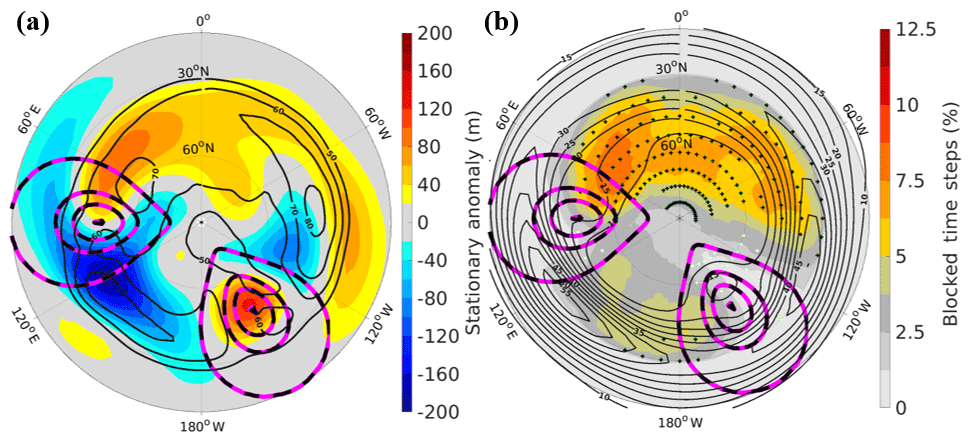
Figure 7 For the two-mountain idealized model integration, (a) the cool-season stationary wave (shading) and storm track (heavy black contours) and (b) the cool-season blocking climatology (shading) and $\stackrel{\mathrm{‾}}{U_{\mathrm{250}}}$ (heavy black contours) are shown. In (a) storm track contours are in 10 m intervals where the outer contour is 50 m. In (b) $\stackrel{\mathrm{‾}}{U_{\mathrm{250}}}$ contours are in 5 m s⁻¹ intervals where the outer contour is 10 m s⁻¹. Black (white) stippling in (b) indicates significantly greater (lower) block frequency at nearby grid points when compared to a 250-year aquaplanet integration. Dotted pink and black contours represent surface height, where the outer contour is the edge of the land mask and the inner contours are in 1 km intervals.

The TwoMtn configuration has a greater hemispherically averaged blocking frequency than the other configurations (Table 2) and is also significantly greater than the aquaplanet. This is despite the TwoMtn configuration having a lower total number of blocks than the 3 and 4 km SingleMtn configurations, respectively – meaning the blocks have a longer average duration in the two-mountain configuration (Table 3). Each mountain also creates regions of enhanced and suppressed blocking frequency (Fig. 7b). However, just like the general circulation features, there are differences in the blocking climatology for the two ocean basins.

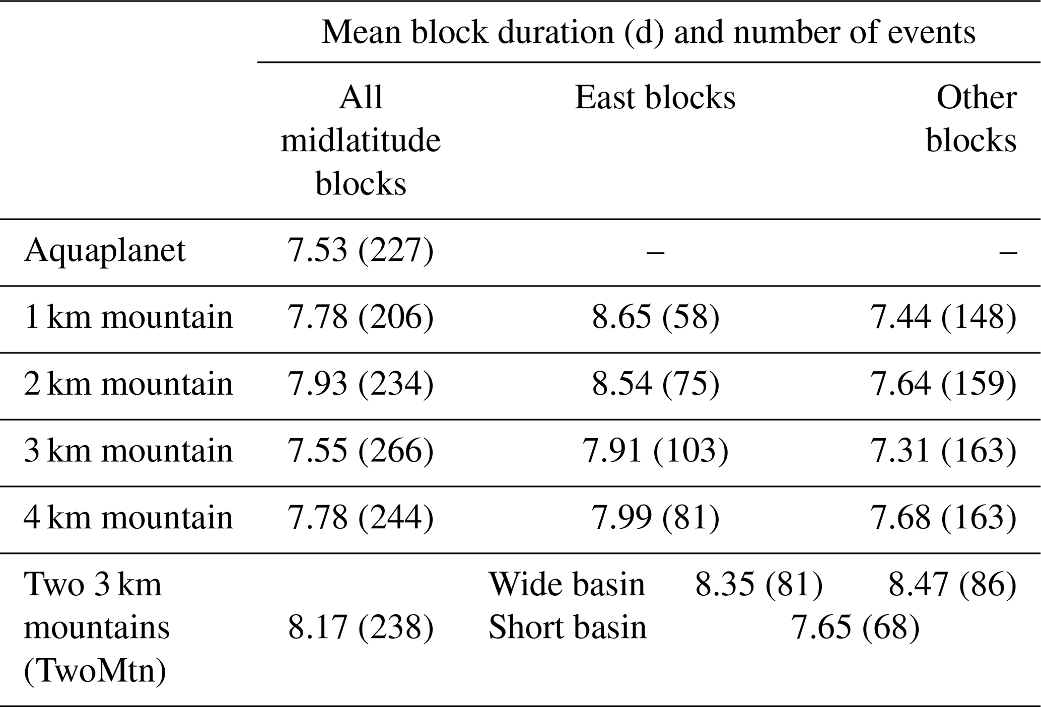
Table 3 Mean block duration and number of events in parentheses for midlatitude, cool-season blocks in each idealized model configuration.

Next, we examine the blocking climatology within each of the two ocean basins in the TwoMtn simulation (wide basin and short basin, respectively; see Fig. 1 and Table 1). In the wide basin, there is close to a basin-wide enhancement of blocking frequency when compared to the single-mountain cases (Figs. 6e–h and 7b). Consistent with this enhancement, the overall midlatitude $\stackrel{\mathrm{‾}}{U_{\mathrm{250}}}$ climatology is much weaker in the wide basin compared to the other ocean basin and SingleMtn integrations. In the short basin, a separate blocking maximum exists near the high-pressure stationary wave anomaly. This maximum, although much weaker than its wide basin counterpart, is still significantly more than what occurs in the same region for the aquaplanet.

The proximity of the storm track maximum in the short basin makes it more likely for there to be times in which storm development occurs just upstream of the mountain; this, coupled with a strong background westerly flow, would inhibit blocking and perhaps explains the discrepancies between the wide basin and short basin maxima. The shorter ocean basin containing much less blocking is not consistent with what is observed in the NH, where the Atlantic has a slightly stronger blocking maximum. It seems more elaborate landmasses than this simplified case are needed to better simulate what is observed between the Atlantic and Pacific blocking climatologies in the NH.

3.3 Block duration statistics

One of the characteristics that allows blocks to influence midlatitude weather is their persistence. As such, we examine the influence of mountains on block persistence using our duration metric. First, we find that adding mountains leads to at least a modest increase in the average midlatitude block duration (Table 3). All topographic configurations aside from 1 km SingleMtn also have 7–39 more blocks than the aquaplanet (Table 3). This helps to explain some of the climatological differences in block frequency between the idealized model configurations (Table 2), particularly for the 1 km SingleMtn case. Despite a 0.25 d greater mean block duration (Table 3), 1 km was found to have less hemispherically averaged blocking than the aquaplanet (Table 2) due to there being 21 less events. The blocks in the topographic integrations were then put into subsets based off those originating near the high-pressure stationary wave anomaly and those that were not.

Regions used to subset blocks are denoted as “East”, those originating at the eastern end of the ocean basin near the high-pressure stationary anomaly, and “Other”, those originating elsewhere in the midlatitudes (Fig. 1a and Table 1). Figure 8 shows the probability density distributions for the aquaplanet and East blocks from each configuration. With the exception of the 4 km run, the East regions of the single-mountain integrations have relatively fewer shorter duration blocks (i.e., 5–11 d) and relatively more longer duration blocks (11 d or more) compared to the aquaplanet (Fig. 8). Blocks from the East regions last longer on average than aquaplanet blocks (Table 3), but the 3 and 4 km enhancement of block duration are not significant to the 95th percentile. Mean block duration is greater for the East region compared to the Other in the single-mountain configurations (Table 3), with significant differences found in the 1 and 2 km integrations. This leads to a cautious suggestion that blocks that originate near mountains last longer on average than those that do not. However, the modest differences found in the 3 and 4 km integrations must be considered, and the nonlinear response of block duration to linear changes in topography attests the system's own internal variability.

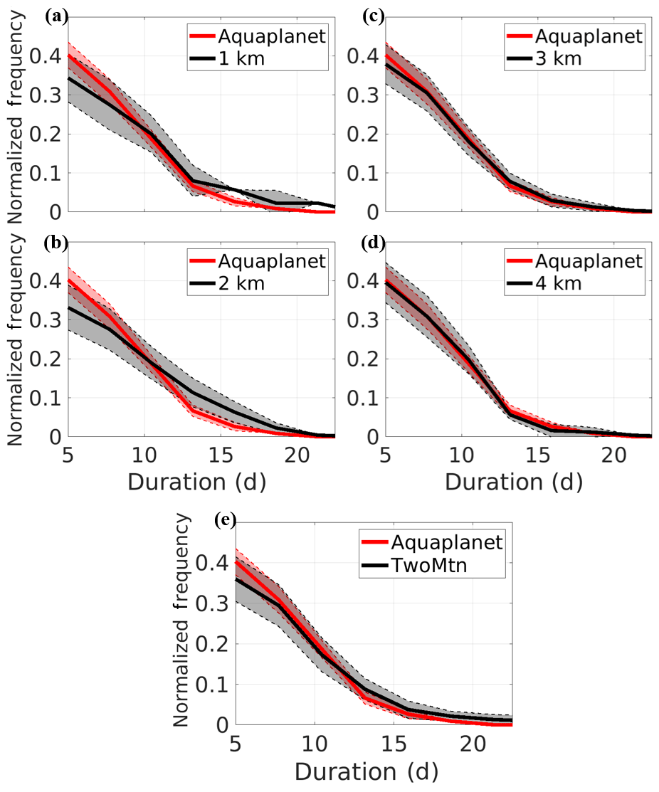
Figure 8 Block duration probability density distributions for the aquaplanet and “East” blocks (as defined in Table 1) in the (a) SingleMtn 1 km, (b) SingleMtn 2 km, (c) SingleMtn 3 km, (d) SingleMtn 4 km, and (e) TwoMtn configurations. Thick lines denote the mean probability density distribution for each configuration. Shaded regions bordered by dotted lines outline ± 1 full standard deviation from the mean.

The response of the TwoMtn configuration is much less straightforward. This integration is divided into three regions, wide basin East, wide basin Other, and short basin (Fig. 1b and Table  ); note that the short basin does not have distinct East and Other regions because of its shortened zonal extent. Average block duration in the Other region in the wide basin is slightly longer than the East region, but both regions are significantly greater than the short basin. This, coupled with more wide basin East events (Table 3), is consistent with the weaker maximum in the blocking climatology for the short basin (Fig. 7b). Perhaps this is related to the inhibition of blocking by the nearby storm track and $\stackrel{\mathrm{‾}}{U_{\mathrm{250}}}$ maximum in the short basin, but we do not seek to attribute a causal relationship here.

Our results suggest that blocks starting near mountains last longer on average than those that do not (Table 3). In reality we see a similar situation where the NH has more orographic forcing compared to the SH and also a longer average block duration (8.0 d for the NH and 6.9 d for the SH). In the idealized model, the compositing analysis for the aquaplanet shows similar forcing patterns by low-frequency eddies (∇⋅W) when compared to the SingleMtn East blocks (Fig. 3d–i), despite having a shorter average block duration. Perhaps these duration differences can be accounted for by considering block maintenance by high-frequency transients (Shutts, 1983; Nakamura et al., 1997; TN01; Yamazaki and Itoh, 2013; Wang and Kuang, 2019). High-frequency eddy forcing has yet to be investigated in these experiments, but this will be a topic of future work.

4 Discussion

To add some perspective on the role of mountains as compared to land masses with no orographic features, we analyze the response of an idealized model configuration with a single flat land mass, herein referred to as 0 km (Fig. 9). The results of 0 km are briefly mentioned here to primarily serve as a benchmark for this setup. This configuration is like the others that include mountains in that it imposes zonally asymmetric forcing in land–sea contrast. The difference, however, is that the flat land does not act as a direct barrier that deflects the flow as the mountains do, generating a unique stationary wave response (e.g., Held et al., 2002) (Figs. 6a–d, 7a, and 9).

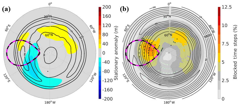
Figure 9 For an integration with one flat landmass, (a) the cool-season stationary wave (shading) and storm track (heavy black contours) and (b) the cool-season blocking climatology (shading) and $\stackrel{\mathrm{‾}}{U_{\mathrm{250}}}$ (heavy black contours). In (a) storm track contours are in 10 m intervals where the outer contour is 50 m. In (b) $\stackrel{\mathrm{‾}}{U_{\mathrm{250}}}$ contours are in 5 m s⁻¹ intervals where the outer contour is 10 m s⁻¹. Black (white) stippling in (b) indicates significantly greater (lower) block frequency at nearby grid points when compared to a 250-year aquaplanet integration. The dotted pink and black contours represent the outer edge of the land mask.

The response of $\stackrel{\mathrm{‾}}{U_{\mathrm{250}}}$ and the storm track (Fig. 9) in 0 km agree with results by Brayshaw et al. (2009). Compared to the single-mountain runs, the stationary wave pattern is shifted upstream in 0 km (Figs. 6 and 9). The blocking climatology maximizes (minimizes) poleward of regions where the midlatitude $\stackrel{\mathrm{‾}}{U_{\mathrm{250}}}$ minimizes (maximizes) (Fig. 9b). In the single-mountain integrations, the maximum in the blocking climatology is nearly co-located with the maximum in the stationary wave; for the 0 km integration, it is not. The high-pressure stationary anomaly seemingly plays less of a role in the flat case. The 0 km integration has a 3.42 % hemispherically averaged block frequency, which is greater than the aquaplanet and 1 km configurations but less than the others with taller mountains (Table 2).

5 Summary and conclusions

This work utilizes an idealized moist GCM to better understand atmospheric blocking. We start with an analysis of blocking in an aquaplanet, then systematically add mountains to investigate the influence of orography on blocking frequency and duration. Below, we recap the answers to the research questions posed in the introduction, followed by concluding remarks.

In regard to question 1, using the aquaplanet we confirm that blocks can be generated without any zonally asymmetric forcing from the surface, consistent with onset governed by eddy–eddy interactions. This result substantiates the results of Hu et al. (2008), Hassanzadeh et al. (2014), and Nabizadeh et al. (2019). To expand on the results of those previous studies, we examined the dynamical life cycle of the blocks in the aquaplanet. Block centered composites of $Z_{\mathrm{500}}^{\prime }$ and W show that block life cycles in the aquaplanet include:

1. large-scale Rossby wave features with W entering the block and converging on the downstream- equatorward flank during onset;

2. stronger W convergence and greater concentrations of W inside the block during peak strength;

3. a net divergence of W emitted downstream of the block into low-pressure regions during decay.

Similar behavior is shown for reanalysis and the idealized model configurations that include orography, affirming the usefulness of a simple idealized aquaplanet model in better understanding blocks observed in reality.

With regards to questions 2–4, in experiments with orographic forcing we modified the aquaplanet model in the following ways: (1) adding a single mountain of different heights in separate integrations; and, (2) in another integration, adding two 3 km high mountains placed in a manner that creates one wide and one short ocean basin. The addition of mountains to the idealized model led to several changes in blocking when compared to the aquaplanet integration.

• There is a significant increase in hemispherically averaged blocking frequency in integrations with mountains of height 2 km and greater (question 2).

• There are localized maxima in blocking upstream of mountains, near the high-pressure maximum of the stationary waves, and poleward and near climatological minima in $\stackrel{\mathrm{‾}}{U_{\mathrm{250}}}$ (question 3).

• There are localized minima in blocking downstream of mountains, near the low-pressure anomaly of the stationary wave, and poleward and near climatological maxima in $\stackrel{\mathrm{‾}}{U_{\mathrm{250}}}$ (question 3).

• There is an increase in block duration for blocks originating near mountains, though the statistics are not robust (question 4).

Based on ERA-Interim reanalysis, these results mirror what is observed for the NH and SH, where the NH contains more topography and blocking. In the idealized model, the enhancement of block frequency near the stationary wave maximum and $\stackrel{\mathrm{‾}}{U_{\mathrm{250}}}$ minimum is consistent with these regions being conducive to the convergence (or “traffic jamming”) of wave activity fluxes. These regions are found to be far from the storm track exit however, which is dissimilar to the NH in reanalysis. At the storm track exit region, previous work has shown that extratropical cyclones can seed blocks (Colucci, 1985) or maintain them (Pfahl et al., 2015). However, in those studies the storm track exit coincides or sits spatially close to the stationary wave maxima. In our single-mountain experiments, the storm track exit is far from the stationary wave maxima, and the result is that the blocks preferentially occur at the stationary wave maxima region. This suggests that the role of the cyclones in nature may be secondary to the role of the large-scale flow. That being said, secondary blocking maxima are found near the storm track exit in the idealized model, suggesting that this location also plays a key role in anchoring where blocks most frequently occur.

We note that the differences in blocking for model configurations with and without mountains is not identical to the differences between the NH and SH in observations. First, from the block-centered composites (Fig. 3), it is clear that the NH versus SH differences in observations for Z₅₀₀ anomalies and wave activity flux are larger than those found for the aquaplanet, as compared to the idealized configurations with orography. This is true for the case shown in Fig. 3 (3 km single mountain) and all other model configurations with orography. Additionally, as compared to the aquaplanet versus idealized model configurations with orography (Figs. 4 and 6), the hemispherically averaged blocking frequency in the NH is much larger than the SH in observations (Fig. 5). That being said, there are important aspects of the climatological blocking frequency in observations that are captured well by the model: there is a minimum at the storm track entrance and maximum near the anticyclonic peak of the stationary wave. For the NH, this behavior is clear in the ocean basins. For the SH, the storm track entrance is difficult to pinpoint, but the blocking minima (Fig. 5d) corresponds with a local maxima in near-surface baroclinicity (Nakamura and Shimpo, 2004).

Differences in blocking between the different idealized model configurations accentuate the primary role of the stationary wave in determining the preferred location of blocking. Furthermore, the fact that the compositing did not show the same differences for aquaplanet versus mountains cases as SH versus NH implies that the subtleties of the block-centered compositing dynamics do not determine the spatial distribution of the blocks. At the same time, secondary blocking maxima at the storm track exits in the single-mountain integrations suggest that synoptic forcing indeed plays an important role in blocking, consistent with the findings of previous work (Colucci, 1985; Nakamura et al., 1997; Yamazaki and Itoh, 2013; Pfahl et al., 2015).

One important caveat to these experiments is that land does not include orographic drag. Pithan et al. (2016) showed that orographic drag plays a key role in the tilting of the North Atlantic storm track and the frequency of European blocking episodes. The absence of drag in these experiments could be a reason for the relatively modest changes in hemispherically averaged blocking statistics, as well as the lack of regional variation in blocking within the idealized model. Furthermore, especially for the TwoMtn experiment, one must keep in mind the highly idealized nature of the orography, which does not contain Greenland or the elongated Eurasian and North American continents. Other differences (i.e., treatment of ocean, etc.) could also play a role in discrepancies in blocking between the idealized and reanalysis models, and more systematic investigation is needed.

Overall, this work elucidates fundamental information on the formation, dynamical evolution, spatial distribution, and duration of atmospheric blocking – both in an aquaplanet and configurations with zonally asymmetric forcing. One limitation in the two-mountain experiment is that each mountain simultaneously affects the stationary wave, jet, and storm track, making it difficult to tell the order of influence each has on the blocking climatology. Understanding the interplay and individual effects of these flow features is key to predicting the behavior of blocks in future climates, which is a topic of future work.