Abrupt transitions in an atmospheric single-column model with weak temperature gradient approximation

We document a feature of the tropical atmosphere that could be relevant to episodes of abrupt transitions in global climate that regularly occurred during the last ice age. Using a single-column model (SCM) incorporating the weak temperature gradient (WTG) approximation, we find that abrupt transitions occur as the sea surface temperature is steadily increased. Because these transitions arise from the interplay between local deep convection and the large-scale adjustments that are required to maintain weak temperature and pressure gradients, they are only present with the WTG approximation relevant for the tropics but may be of interest as a trigger for abrupt transitions in global climate. These transitions are marked by an abrupt change in the partitioning of rainfall between convective and large-scale (microphysics) subroutines in addition to various other features of the column, including cloudiness, vertical velocity, temperature, and humidity. We conclude that the transitions are initiated by a failure of evaporative cooling in the lower free troposphere. This leads to lower-column heating and a burst of convection that heats the upper free troposphere, increasing the large-scale rainfall rate, which allows for sufficient evaporative cooling to restabilize the column.

1 Introduction

Explanations for abrupt climate change during the last ice age have largely focused on the role of the ocean, particularly the Atlantic meridional overturning circulation sensitivity to a freshening of the North Atlantic (Clark et al., 2002; Jackson et al., 2010). It is not yet clear whether this mechanism is sufficient to explain observed changes in tropical climate, particularly its hydrologic cycle and its monsoons (Peterson et al., 2000; Wang et al., 2001; Cruz et al., 2005; Weldeab et al., 2007; Clement and Peterson, 2008; Stager et al., 2011). Previous experiments with advanced climate models (Okumura et al., 2009) that have tested the freshwater forcing hypothesis do not contain the sensitivity required to explain the 40 % reduction in atmospheric methane associated with cold stadials, an observation interpreted to reflect large reductions in tropical wetland extent (Brook et al., 1996, 2000; Fischer et al., 2008), although there may be complications in that interpretation (Kaplan, 2002; Kaplan et al., 2006). There is a need to explore more broadly how and why abrupt transitions in global climate have occurred, especially mechanisms within the tropical atmosphere (Wunsch, 2006; National Research Council, 2013).

Several studies document a relationship between sea surface temperature (SST) and either multiple equilibria or qualitative differences in rainfall behavior. Sobel et al. (2007) and Sessions et al. (2010) both find that rainy and dry states exist for the same boundary conditions under the weak temperature gradient (WTG) approximation designed by Sobel and Bretherton (2000) to parameterize large-scale tropical dynamics for limited-domain models. Using a single-column model (SCM), Sobel et al. (2007) find the existence of dry and rainy states to be sensitive to both SST and the horizontal moisture advection rate, while Sessions et al. (2010) find similar behavior in a cloud-resolving model. These multiple equilibria have been understood in the context of explaining the spatial structure of tropical rainfall, but the fact that different equilibria exist under the WTG approximation is also interesting in the context of abrupt climate change. Held et al. (2007) also find that warmer SSTs are associated with qualitatively different types of rainfall behavior. Using a large, doubly periodic, nonspherical and nonrotating domain run at typical general circulation model (GCM) resolution with an initialization appropriate for the tropics, Held et al. (2007) document higher fractions of large-scale rainfall and the appearance of what they call “gridpoint storms” – areas sometimes spanning multiple grid cells generating predominantly large-scale (as opposed to parameterized convective) rainfall – for higher SSTs.

In this paper, we find that under a simple forcing, namely a continuous increase in SST, the single-column mode of the Weather Research and Forecasting (WRF) model responds by abruptly transitioning to new configurations, with important consequences for rainfall. Rather than rainy and dry states, however, our experiments demonstrate the existence of multiple equilibria in the relative amounts of convective and large-scale rainfall. These transitions only occur when the WTG approximation is implemented in the columns, making the transitions of interest in the tropics. Because the fraction of large-scale rainfall correlates strongly with circulation and spatial rainfall patterns, including in the response to CO₂ forcing (Stephens et al., 2019), understanding these transitions and what role they may play in global climate models is worthy of investigation.

2 Experimental setup

The single-column model used in this study is the Weather Research and Forecasting (WRF) model version 3.5, compiled in single-column mode and modified by Wang and Sobel (2011) to implement the WTG approximation. SCMs generally do not account for interactions between local processes and large-scale dynamics; therefore the WTG approximation is useful because it restores the coupling between convection and large-scale dynamics in the less computationally expensive SCM setting. Under the WTG approximation, the resolved vertical motion, rather than being set to zero or some specified velocity profile, is calculated to keep free-tropospheric temperatures close or equal to a temperature profile representing radiative-convective equilibrium (RCE). The justification for the WTG approximation lies in geostrophic balance, which for the tropical free troposphere implies small horizontal pressure and temperature gradients (Charney, 1963) due to gravity waves quickly eliminating pressure and temperature anomalies (Bretherton and Smolarkiewicz, 1989).

The equations governing the evolution of potential temperature θ and the water vapor mixing ratio q in the WRF SCM with the WTG approximation are

$$\begin{array}{}\text{(1)}& {\displaystyle \frac{\partial \mathit{\theta }}{\partial t}}=W+Q_{\mathrm{r}}^{\mathit{\theta }}+Q_{\mathrm{c}}^{\mathit{\theta }}+Q_{\mathrm{s}}^{\mathit{\theta }}+Q_{\mathrm{m}}^{\mathit{\theta }}+Q_{\mathrm{b}}^{\mathit{\theta }}\text{ and}\end{array}$$

$$\begin{array}{}\text{(2)}& {\displaystyle \frac{\partial q}{\partial t}}=-\mathit{\omega }{\displaystyle \frac{\partial q}{\partial p}}+Q_{\mathrm{c}}^q+Q_{\mathrm{s}}^q+Q_{\mathrm{m}}^q+Q_{\mathrm{b}}^q,\end{array}$$

where all variables are functions of time t and height z (or pressure p). There are different ways to implement the WTG approximation in practice (for an “intercomparison” study exploring different methods and models for coupling convection to large-scale dynamics, see Daleu et al., 2015). One approach is to assume that the tropical free-tropospheric temperatures do not evolve in time at all (i.e., $\partial \mathit{\theta }/\partial t=\mathrm{0}$), but here the WTG approximation is implemented via “Newtonian relaxation”, meaning instead of holding free-tropospheric temperatures fixed, they are continuously nudged back toward a target vertical temperature profile θ_RCE on some timescale τ. W in Eq. (1) represents the WTG Newtonian relaxation back to the RCE “background” profile θ_BG,

$$\begin{array}{}\text{(3)}& W=-{\displaystyle \frac{\mathit{\theta }-{\mathit{\theta }}_{\mathrm{BG}}\left(z\right)}{\mathit{\tau }}}=-\mathit{\omega }{\displaystyle \frac{\partial \mathit{\theta }}{\partial p}}.\end{array}$$

As with the column resolution, a range of WTG relaxation timescales were tested, but the primary experiments were carried out with τ=180 min. The remaining forcing terms in Eqs. (1) and (2) are from radiation (subscript “r”), the deep-convective parameterization (“c”), the shallow-convective parameterization (“s”), cloud microphysics (“m”), and the boundary layer parameterization (“b”). (As a practical matter, within the WRF code, the WTG forcing W in Eq. (1) is combined with the boundary layer forcing $Q_{\mathrm{b}}^{\mathit{\theta }}$, but they can be separated again later for analysis.) Equation (3) allows the program to solve for the vertical pressure velocity ω, which is then used to evaluate the term $-\mathit{\omega }\frac{\partial q}{\partial p}$ in Eq. (2).

As mentioned above, it is possible to implement the WTG approximation such that the WTG term W exactly cancels the other forcing terms, and the change in temperature is zero. Here, because the WTG relaxation term is not constrained to exactly balance the diabatic forcing terms, the potential temperature at a given height or pressure level will depart from the background value in proportion to the total diabatic forcing at that level. Hence if ∑Q were to abruptly increase at a given height, the quasi-stationary temperature at that height would abruptly increase as well, despite the WTG relaxation scheme. A further complication arises from the fact that the WTG approximation does not counter the diabatic heating everywhere, but only in the free troposphere, defined here as levels above 850 mb. Below the free troposphere in the boundary layer, the vertical velocity is reduced linearly from its value at p=850 mb to zero at the ground.

Here we carry out WRF model experiments based on the Community Atmosphere Model (CAM) version 3.0 physics parameterizations, including for radiation, microphysics (Morrison and Gettelman, 2008), deep (Zhang and McFarlane, 1995) and shallow convection (Park and Bretherton, 2009), and boundary layer processes (Bretherton and Park, 2009). A complete description of the WRF model version 3.5 can be found on the University Corporation for Atmospheric Research (UCAR) website (Skamarock et al., 2008).

For radiation purposes, we set the column at a latitude of zero degrees. Because cloud-radiation feedbacks can complicate the interaction between convection and large-scale advection (which the WTG approximation is usually employed to study), WTG experiments often make use of prescribed radiative cooling such that the column cools via emission of longwave radiation at a rate matching tropical observations (Daleu et al., 2015). The WRF model as modified by Wang and Sobel (2011) includes this option of idealized cooling in the troposphere (they use a rate of −1.5 K d⁻¹). Because we are interested in how the standard CAM physics parameterizations behave under SST forcing, we use the realistic CAM radiation scheme in our primary experiments, though with no seasonal cycle. We have also tested the forcing under prescribed radiation, however, and we comment on those results below. As Wang and Sobel (2011) note, ice clouds in the upper troposphere can block outgoing radiation in a realistic tropical setting, an effect they do not account for but which is important in this study.

In testing these results' sensitivity to various model settings, a range of horizontal and vertical resolutions were ultimately used, but the standard SCM setup was for a 100 km horizontal resolution (WRF's single-column mode runs on a 3×3 stencil, and hence a horizontal resolution must be specified; we chose a resolution similar to that of a typical GCM) and 50 vertical levels up to a height of 20 km. The time step was set to 5 min.

We use the fraction of large-scale rain generated by the model as a basic diagnostic. Like a typical global atmospheric model, the WRF model generates both convective and large-scale rainfall (the latter is usually called “nonconvective” rain in the WRF context). In Stephens et al. (2019), f_LS was defined as the tropical (30^∘ S–30^∘ N) mean large-scale rainfall rate divided by the tropical mean total rainfall rate $f_{\mathrm{LS}}\equiv \sum P_{\mathrm{LS}}/\sum (P_{\mathrm{LS}}+P_{\mathrm{C}})$, where the total convective rain rate P_C included shallow-convective rainfall. Since here we are using a simpler one-dimensional model that does not automatically sum deep and shallow-convective rain, f_LS is defined as

$$\begin{array}{}\text{(4)}& f_{\mathrm{LS}}\equiv {\displaystyle \frac{P_{\mathrm{LS}}}{P_{\mathrm{LS}}+P_{\mathrm{D}}+P_{\mathrm{SH}}}},\end{array}$$

where P_LS, P_D, and P_SH are the SCM large-scale, deep-convective, and shallow-convective rainfall rates, respectively.

The SST-forcing experiments analyzed in this paper were all done similarly. Using 300 K as a typical tropical SST, the WRF SCM is first run to radiative-convective equilibrium with this surface temperature over a period of 180 d. The final 30 d of this experiment are then averaged to extract equilibrated pressure, temperature, height, and humidity profiles, which are then used to determine the background profile θ_BG for the WTG routine (Eq. 3), and then the experiments are started again at 300 K with the WTG approximation active. After an initial 90 d startup, the SST is continuously increased at a fixed rate (usually 0.5 K per month; varying the rate of SST increase or decrease does not have a strong effect on the SCM's behavior) for sufficient time to reach a specified maximum temperature (usually 304 K). The temperature is then held at the maximum value for a period of 90 d and then continuously reduced back to 300 K, where the SST is held for a final 90 d period. The experiments are all initialized with the same temperature and moisture profiles consistent with an SST of 300 K.

3 Findings

This section is divided into four subsections. In the first, we describe general observations we have made using the WRF SCM with and without the WTG approximation, including the rainfall behavior for both cases and how the column balances the temperature and moisture forcings in each case. In the second subsection, we document the hysteresis and multiple equilibria we have found within the column under the WTG approximation with SST forcing, and in the third subsection we describe in greater detail the abrupt transitions that have been our primary focus (to be further analyzed in the following Discussion section). In the final subsection, we briefly describe a unique state, characterized by f_LS=1, into which the column sometimes abruptly transitions and from which it never seems to recover.

3.1 RCE vs. WTG experiments: general observations

We begin by describing the typical features of our WRF SCM radiative-convective equilibrium experiments and how these experiments are typically affected by activating the WTG approximation without anomalous SST forcing. Figure 1 displays tropical temperature, humidity, and cloud profiles averaged from the last 30 d of two 180 d WRF SCM experiments: one a radiative-convective equilibrium experiment and one using the WTG approximation. The temperature plot includes ERA-Interim reanalysis data for reference. Figure 1 shows several important effects of the WTG approximation: along with significantly increasing the free tropospheric moisture, it induces strong, large-scale upward motion and hence condensation, causing large cloud fractions in the upper column. The warming effect of this condensation above ∼700 mb is evident in the temperature sounding for the WTG experiment, although the highest parts of the column show cooling. While the large cloud fractions are unrealistic, they are a persistent feature of WTG experiments using the (realistic) CAM radiation parameterization.

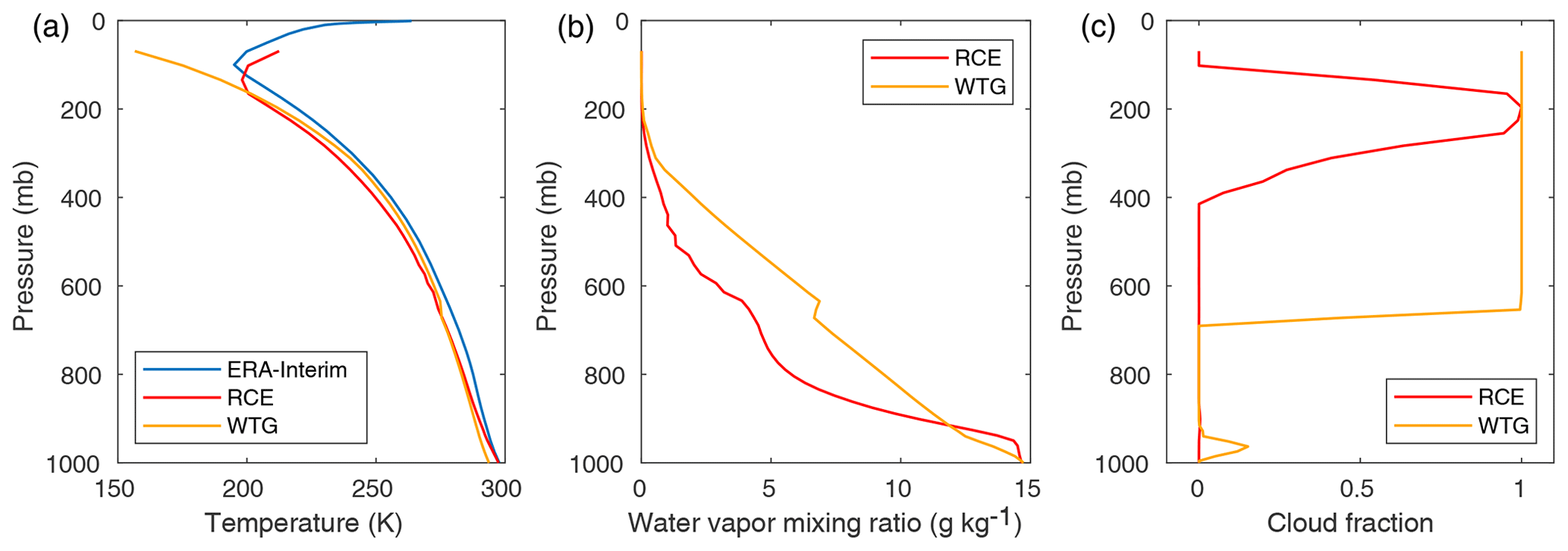
Figure 1 (a) Tropical soundings from ERA-Interim reanalysis (observational) data and averages over the last 30 d of two 180 d WRF SCM experiments: one an RCE experiment and one with the WTG approximation active, both with fixed 300 K SST. (b) Water vapor mixing ratio profiles from the same RCE and WTG experiments. (c) Cloud fraction profiles from the same RCE and WTG experiments.

Figure 2 (a, b) Column profiles of the potential temperature (θ) forcings from Eq. (1) averaged over the last 30 d of RCE (a) and WTG (b) experiments, both run for 180 d with fixed SST of 300 K. The forcings are from the deep-convective (blue), shallow-convective (green), boundary layer (black), radiative (cyan), and microphysics (red) CAM parameterizations and the WTG relaxation scheme (orange). (c, d) Column profiles of the water vapor mixing ratio (q) forcings for the same two experiments. The WTG background profile was calibrated to an SST of 300 K.

Figure 3 (a) The left axis shows f_LS for the WRF SCM over 800 d RCE (blue) and WTG (black) experiments. When running the SST-forcing experiment in an RCE configuration, the unfiltered f_LS has an average value of ∼0.28 and a standard deviation of ∼0.18. (The presented RCE f_LS data have been low-pass filtered for clarity.) (b) The left axis shows convective (blue) and large-scale (black) rain rates for the RCE experiment. These data have been low-pass filtered. (c) The left axis shows convective (blue) and large-scale (black) rain rates for the WTG experiment. The right axes for all plots give SST over the experiments.

Table 1 A series of quantities averaged over the last 30 d from 180 d RCE and WTG approximation experiments without anomalous SST forcing. After f_LS, the three types of precipitation (deep-convective P_D, large-scale P_LS, and shallow-convective P_SH) are shown, followed by the shortwave radiation to the surface (SWD), the outgoing longwave radiation from the ground (GLW), the outgoing longwave radiation at the top of the column (OLR), and the surface sensible (HFX) and latent (LH) heat fluxes.

The way the column balances the various forcing terms of Eqs. (1) and (2) changes dramatically when the WTG approximation is active. In the RCE case (Fig. 2, panels a and c), the dominant θ-forcing balance over a large part of the column is between convective heating and radiative cooling, and Eq. (1) becomes $Q_{\mathrm{r}}^{\mathit{\theta }}\approx Q_{\mathrm{c}}^{\mathit{\theta }}$. Meanwhile, the q-forcing terms are small above roughly 800 mb, with the convective and boundary layer schemes balancing each other below that level. With the WTG approximation active (Fig. 2, panels b and d), the balances are qualitatively and quantitatively different. Qualitatively, the WTG column now shows two different kinds of balance for the upper and lower troposphere. Above roughly 600 mb (the height of the cloud base), the dominant balance is between heating from condensation (microphysics) and cooling from the WTG relaxation, W≈Q^θm. In the lower column, the dominant balance is between convective heating and evaporative cooling (also microphysics), $Q_{\mathrm{m}}^{\mathit{\theta }}\approx Q_{\mathrm{c}}^{\mathit{\theta }}$, with shallow convection and the WTG relaxation playing more minor roles. Radiation plays a comparatively minor role in the WTG case, a consequence of the noted extreme cloudiness of the upper column; infrared radiation from below is absorbed at the cloud base, and longwave radiative cooling dominates at the top of the column, while shortwave radiation from space is almost all absorbed by high-level clouds (Table 1). Because of this, evaporation from the microphysics parameterization is the only available source of cooling in the lower column and plays a critical role in the abrupt transitions described below. As panels c and d of Fig. 2 show, the moisture forcings largely follow the θ forcings in the WTG case and indicate the much more important role played by moisture when the WTG approximation is active.

Quantitatively, the magnitudes of the forcings are much larger with the WTG approximation active, likely a consequence of a positive heating feedback active in the upper column (discussed further in the Discussion section). Of particular interest in this connection is the fact that while mixing via deep convection is now largely restricted to p≳650 mb – probably because of the reduced lapse rate and hence stabler profile near that level (see Fig. 1) – the deep-convective θ forcing is much larger than in the RCE experiments. The greater convective heating cannot be attributed to greater convective available potential energy (CAPE), which is much larger in the RCE case, wherein the upper column is cooler. Rather, the greater deep-convective θ forcing is likely due to the greater abundance of moisture and therefore larger condensational heating as convective plumes rise into cooler air.

Considering the very different temperature and moisture forcing balances within the column, it is unsurprising that the RCE and WTG cases show different rainfall behavior, both in rainfall rates and type (Table 1). Using the CAM physics options, a typical f_LS for the standard WRF SCM is about 0.3, while with the WTG approximation active f_LS is generally larger due to the greater upper-column microphysics activity.

Table 2 Average values for a series of quantities for the two distinct SCM equilibria (E1 and E2) shown in Fig. 4. After f_LS, the three types of precipitation (deep-convective P_D, large-scale P_LS, and shallow-convective P_SH) are shown, followed by the shortwave radiation to the surface (SWD), the outgoing longwave radiation at the top of the column (OLR), and the surface sensible (HFX) and latent (LH) heat fluxes.

The column response to increasing SST is very different with and without the WTG approximation active. As Fig. 3 shows, in the RCE case, an increasing SST leads to greater intensity of rainfall while reducing f_LS slightly. As the SST is decreased again, this pattern reverses. On the other hand, with the WTG approximation active, as SST increases the column begins to show stepwise abrupt transitions to larger f_LS, a robust outcome of such experiments (apart from the possible f_LS→1 behavior discussed below). It is apparent that when the column is run without the WTG approximation, higher SSTs result in greater convection, but with the WTG approximation active, the presence of a large-scale vertical pressure velocity ω allows the column an additional means of handling the upward redistribution of energy.

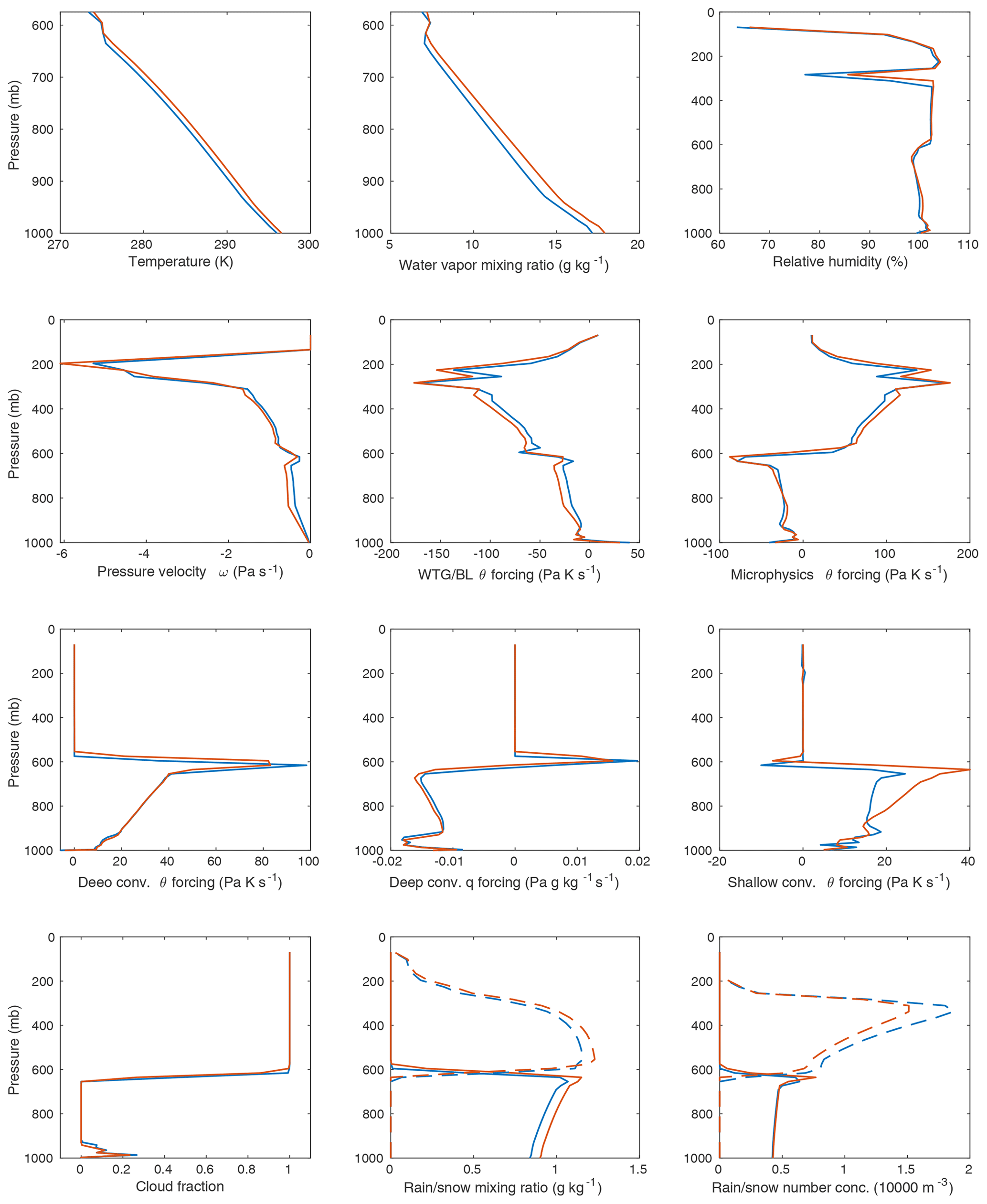
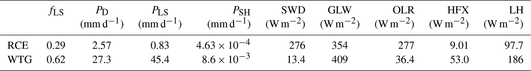
Figure 4 Average profiles for a number of variables for two SCM solutions at SST 304.5 K. Blue represents E1 (the equilibrium obtained during the warming phase), and red represents E2 (the cooling phase equilibrium). Forcing terms are mass-weighted in WRF, hence the units of pascals times kelvin per second. Note that the WTG forcing is combined with the boundary layer forcing here, but this quantity is dominated by the WTG forcing above the boundary layer. In the plots for rain or snow mixing ratio and number concentration, solid lines represent rain, and dashed lines represent snow. See also Table 2.

3.2 Hysteresis and multiple equilibria

Figure 3 confirms that with the WTG approximation active, the column exhibits hysteresis: the evolution of f_LS as the column warms is different from its evolution as the column cools. To document the implied multiple equilibria, we carried out a modified version of the experiment described in Sect. 2, wherein we began the temperature increase at 300 K as before, paused the SST increase at a “resting” SST of 303.5 K, allowed the model to run for 30 d at the resting SST, then continued the temperature increase to 304 K. We then allowed the model to rest for another 30 d at the same resting SST during the cooling phase.

Table 2 and Fig. 4 document two different SCM solutions averaged over those 30 d resting-SST periods, which we call E1 and E2. E1 is the solution obtained during the warming phase of the experiment, and E2 is obtained during the cooling phase. It is evident from Fig. 4 that in the case of E2, the model has settled into a warmer, wetter solution with stronger vertical motion, although there is nuance in how the model achieves balance between heating and cooling in this case relative to E1. The clearest difference is in the shallow-convective subroutine, where for E2 shallow convection plays a much greater role in heating the column between roughly 900 and 600 mb, while the rate of shallow rainfall P_SH (while small compared to deep-convective or large-scale rain) more than doubles (Table 2). Both deep and shallow convection also reach slightly higher into the column for E2. E2's enhanced shallow-convective heating is offset between 900 and 650 mb by both the WTG relaxation and evaporative cooling from the microphysics scheme; it is noteworthy that the microphysics parameterization is unable to balance the lower-column heating alone. Near 600 mb, however, E2 shows a net increase in heating from shallow convection. The deep-convection q forcing shows that the E2 solution is furthermore removing more vapor from below 600 mb and depositing slightly more above.

3.3 Abrupt transitions and quasi-stationary states

The results described in this section and analyzed in the Discussion section below are taken from an RCE experiment at an SST of 300 K and an SST-forcing experiment increasing the temperature from 300 to 304 K with a rate of increase of 0.5 K per month. The average f_LS for the last 30 d of the 180 d RCE experiment is 0.28. The WTG experiment first equilibrates with an f_LS of about 56.0 %, but as the SST is increased, the column shows three abrupt transitions to higher f_LS, roughly 62.7 %, 64.5 %, and finally 66.1 % (Fig. 5, upper left panel). As noted, the column shows additional abrupt behavior and hysteresis as SST is decreased, but a close analysis of the cooling phase is left for future work.

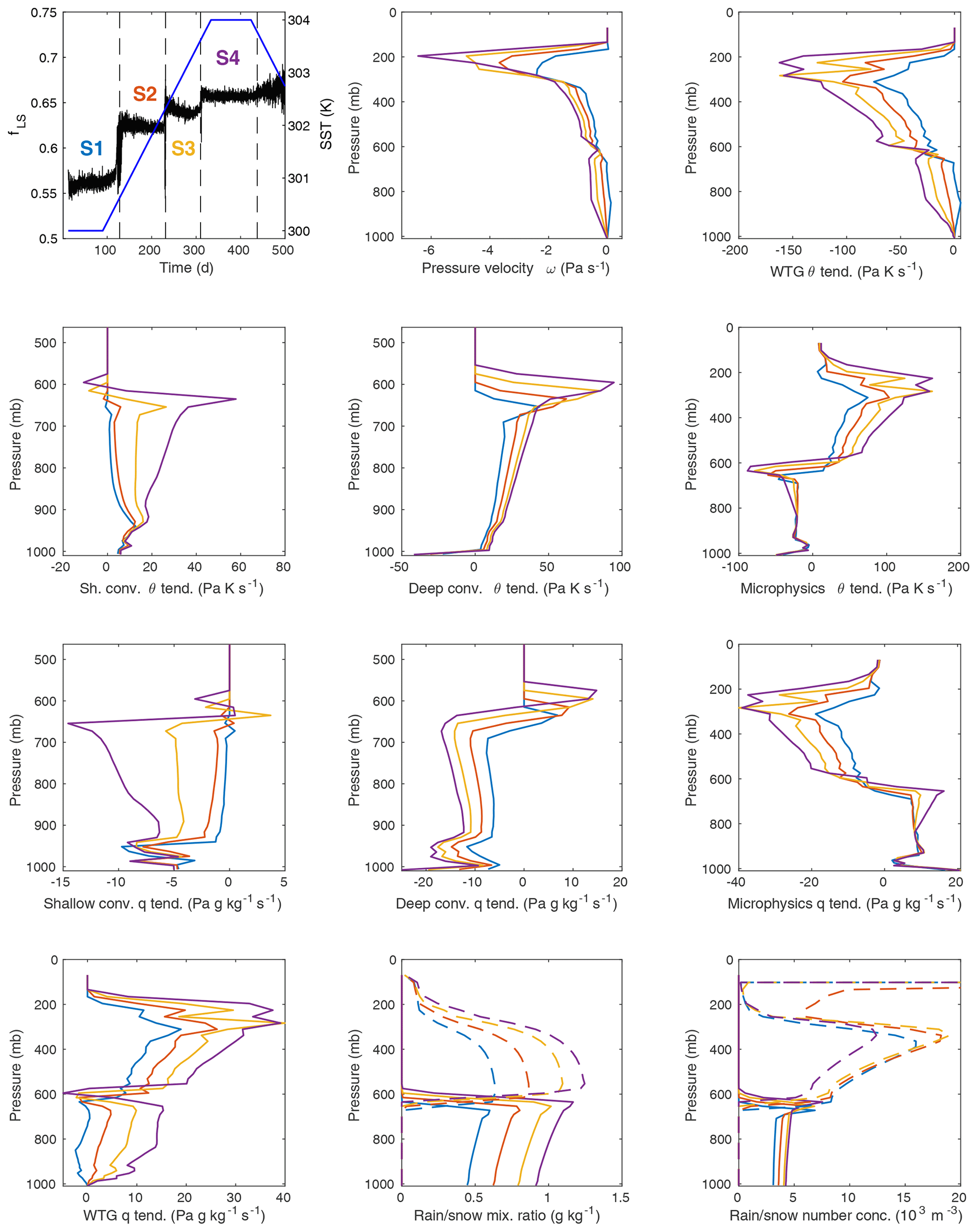
Figure 5 Four quasi-stationary states of the heating WRF SCM with WTG approximation. For the top left plot, the left axis shows f_LS for the WRF SCM over the first 500 d of an 800 d integration with the WTG approximation active and a background profile calibrated for 300 K SST. Four quasi-stationary states (S1, S2, etc.) are indicated. The right axis shows SST over the same integration. The remaining plots show vertical profiles for the labeled quantities, averaged over time for each of the four states (S1 blue, S2 red, S3 yellow, S4 purple). The four plots showing convective forcing profiles stop near 500 mb because they are zero above. WRF model forcings are mass-weighted, hence the units in terms of pressure. In the last two plots for rain or snow mixing ratio and number concentration, the solid lines represent rain and the dashed lines represent snow. See also Table 3.

Figure 5 and Table 3 show both the evolution of f_LS as the WRF SCM heats up and the major characteristics of the four quasi-stationary states (S1, S2, etc.) observed before and after the abrupt transitions. It is clear from the profiles of ω, the various θ- and q-forcing terms, and the rain and snow mixing ratios and number concentrations that, in general, the magnitudes of upward motion, heating, moistening, and rainfall grow as the surface temperature increases. There are, however, some features that show interesting qualitative changes as one state gives way to another. In particular – and as noted above in discussing the multiple equilibria at 304.5 K – the shallow-convection profile shows the most marked change, with both the magnitude and shape of its profile changing from state to state, with progressively greater activity higher above the surface. Moreover, both the deep and shallow-convective profiles reach higher into the column for higher SST. (Consistent with this observation, the cloud base moves higher with each transition.)

Table 3 Average values for a series of quantities for the four states from the experiment shown in Fig. 5. After f_LS, the three types of precipitation (deep-convective P_D, large-scale P_LS, and shallow-convective P_SH) are shown, followed by the shortwave radiation to the surface (SWD), the outgoing longwave radiation from the ground (GLW), the outgoing longwave radiation at the top of the column (OLR), and the surface sensible (HFX) and latent (LH) heat fluxes.

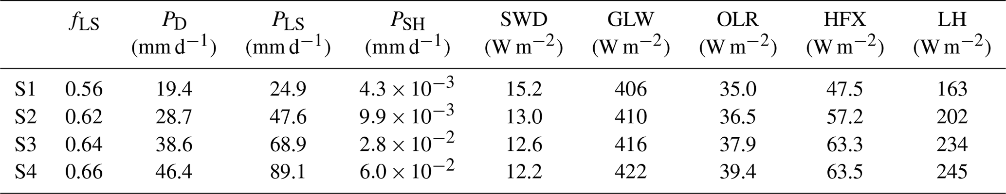
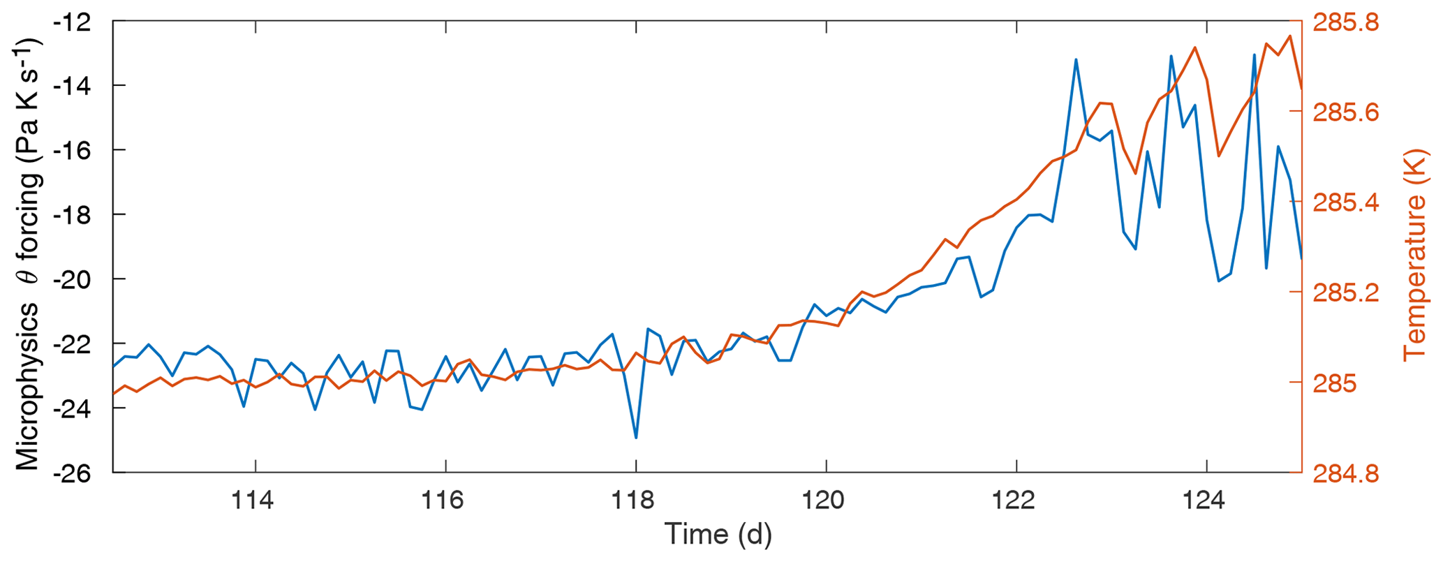
Figure 6 Left axis: the microphysics θ forcing at roughly 835 mb (blue) during the first abrupt transition. Right axis: the temperature at the same level (red).

Before looking closely at the abrupt transitions, it is worth noting some general features of the column evolution leading up to the transitions. As expected, temperatures near the surface begin to increase along with the SST forcing, but, for example, the temperature one level above the surface increases at only 0.15 K per month, much slower than the 0.5 K per month SST increase. (For comparison, in an identical SST-forcing experiment without the WTG approximation, the temperature one level above the surface increases at 0.46 K per month.) Also as expected, given the way the WTG approximation is designed to operate, as the height approaches p=850 mb, where the WTG relaxation becomes active, temperatures are more stable. More surprising, however, is the column behavior above roughly 650 mb. Here, temperatures increase even more quickly than near the surface (e.g., at a rate of roughly 0.35 K per month at p≈460 mb, with some higher levels showing even larger warming rates). This can only be an effect of the convective parameterizations removing heat from near the surface and moisture from throughout the lower column and depositing both near 650 mb (see Figs. 2 and 5), where the large-scale advection generated by the WTG relaxation takes over, carrying this moisture aloft into cooler air, where the microphysics generate the observed condensational heating. Moreover, convection is delivering this heat and moisture to the upper column at a growing rate; if the rate were constant, the WTG relaxation could stabilize the temperatures. This increasing rate of heat export from near the surface is probably consistent with the fact that the surface is heating so much more slowly than it would in the absence of the WTG relaxation. This general behavior causes the more stable “middle” part of the column, between roughly 900 and 650 mb, to grow increasingly out of sync with the regions heating above and below.

A close look at the abrupt transitions shows some features common to all. First, the forcing that most closely follows the lower-column heating is the microphysics, and within the microphysics routine it seems clear that a loss of evaporative cooling is the main driver of the rapid temperature increase at the transition. In the standard model output, this relationship is especially clear during the first transition (Fig. 6). And while the microphysics forcing grows noisier as SST rises, making the relationship slightly less clear in the standard output for the second and third transitions, unprocessed, high-resolution output obtained from the microphysics routine confirm the same pattern for the second and third transitions as well (not shown). As the evaporation starts to fail and temperature starts to increase, a new positive feedback develops: the WTG relaxation responds with cooling and stronger upward motion, advecting moisture upward and causing the mixing ratio and relative humidity to rapidly increase alongside temperature, despite the falling evaporation and likely exacerbating the evaporation shortfall. Moreover, the WTG relaxation plays a progressively greater cooling role in the lower column with each transition, while the microphysical cooling recovers but does not gain much ground between roughly 700 and 900 mb over the course of the SST forcing (see Fig. 5). It is possible that generally high relative humidity in the lower column limits evaporative cooling such that as the column warms, the microphysics ultimately cannot provide enough cooling to balance the heating from the convective routines. Growing local relative humidity, and therefore less ability to take up additional water vapor, might even be suggested as a trigger for the transition, but the relative humidity does not increase markedly before the first transition and is smoothly decreasing before the onset of the second and third transitions, most likely because the convective routines are quickly removing moisture from the lower column.

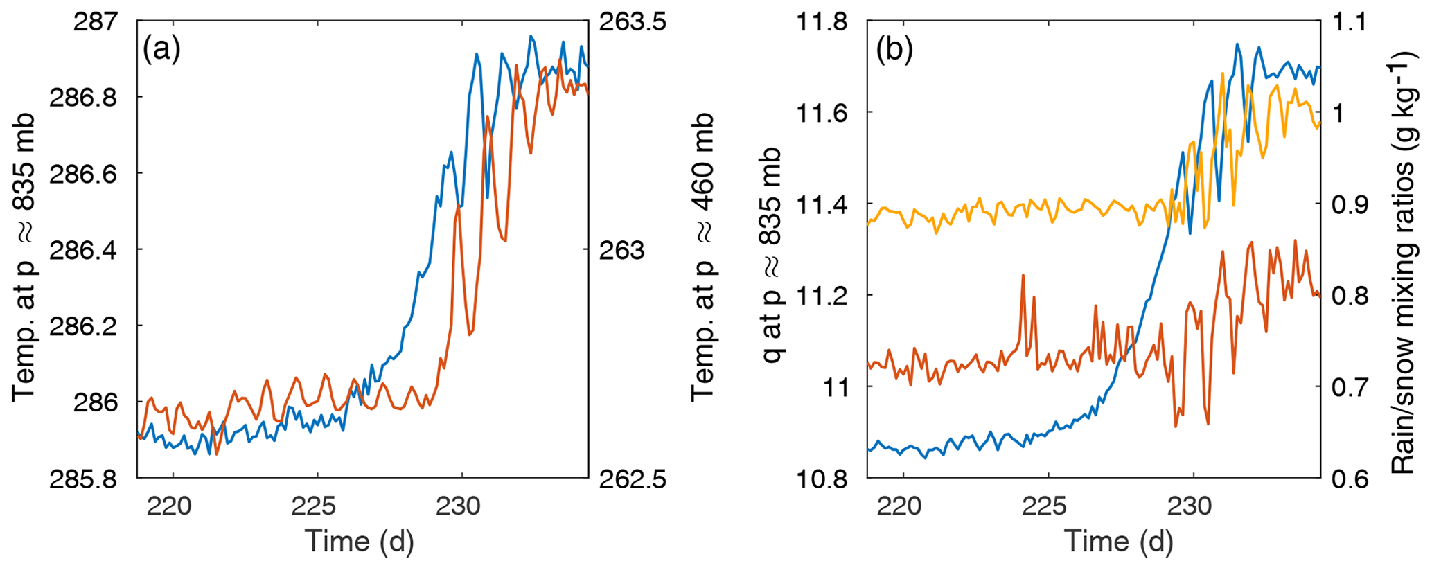
Figure 7 (a) Left axis (blue): temperature (T) evolution at a randomly selected level from the lower part of the column (p≈835 mb). Right axis (red): temperature evolution at a randomly selected level from the upper part of the column (p≈460 mb). (b) Left axis: water vapor mixing ratio (q) evolution at p≈835 mb (blue). Right axis: the rain (red) and snow (yellow) mixing ratios' evolution at p≈835 and p≈460 mb, respectively. The evolution of the latter (microphysics) variables is largely determined by the upper column.

Second, the upper and lower parts of the column experience the transitions differently. As seen in Fig. 7, over the few days during which a transition takes place, the upper-column temperatures temporarily stabilize (or even slightly decrease), while the lower-column temperatures show a rapid but fairly smooth increase. Consistent with this, the upper-column diabatic heating and WTG relaxation also temporarily stabilize or reverse their trends. Toward the end of the rapid temperature and moisture increase in the lower troposphere, the corresponding upper-column variables abruptly transition to new values. For clarity and simplicity, we refer to these two types of transition behavior as “rolling” for the lower column and “snapping” for the upper column.

Third, it seems clear that the transition's transmission to the upper column and termination are closely connected to the convective parameterizations: the convective scheme's θ and q forcings briefly spike near the end of the lower-column “roll” just as the upper-column variables “snap” into their new quasi-stationary values. These are among the rare occasions when the convective routine is able to penetrate above ∼600–650 mb, and after this burst of convection near the end of each transition, convective mixing reaches (usually one level) higher into the column than before. Aside from these spikes at the transitions, the deep-convective forcings grow quite linearly with SST.

Finally, while most variables follow the behavior of their corresponding part of the column (i.e., most lower-column variables show rolling behavior, while most upper-column variables show snapping behavior), some variables do not. The convective routines are one example, but the rain and snow mixing ratios (determined by the microphysics parameterization) also break the pattern, showing snapping behavior even in the lower column (Fig. 7, panel b). This is consistent with precipitation changes initiated in the upper column subsequently becoming apparent in the lower column as the rain and snow precipitate out.

In some cases, there are sudden changes in certain variables prior to the transitions, although a causal relationship is not clear. The most intriguing of these precursor events involve abrupt changes in the mixing ratios and number concentrations of water (lower column) and/or ice (upper column). These shifts may signal threshold-crossing behaviors in the microphysics subroutine as it responds to the heating environment. Figure 8 gives an example of this type of precursor behavior for the second and third abrupt transitions. In panel a, the rainwater number concentration N_r is shown against the temperature evolution; N_r clearly shifts abruptly at t≈180 d, again at the first temperature transition, and then there is another possible shift at t≈275 d before the second temperature transition. In panel b of Fig. 8, the rainwater mixing ratio q_r is shown against the water vapor mixing ratio. Again, it appears q_r shifts near t≈180 d, although a shift is less evident near t≈275 d. However, these plots are for one level only (around p≈835 mb) and are not representative of the entire column. The microphysics variables show rich behavior that is often difficult to interpret – no doubt a consequence of the richness of the microphysics routine, described briefly in the next section – but it is worth noting that the changes depicted in Fig. 8 do seem to coincide with the initiation of a slow temperature increase leading up to the transitions, clearer in the second and especially third transition than in the first. This may imply correlation or causation, but caution is warranted.

Figure 8 Potential precursor activity for the second and third abrupt transitions. (a) Left axis: temperature (T) evolution (blue). Right axis: raindrop number concentration evolution (red) with low-pass filtering shown in black. (b) Left axis: water vapor mixing ratio (q) evolution (blue). Right axis: the rainwater mixing ratio evolution (red) with low-pass filtering shown in black. All quantities are at p≈835 mb.

3.4 The f_LS→1 case

Under certain conditions, the WRF SCM under the WTG approximation can transition into a state with f_LS=1. In this state the convective parameterizations shut down completely, the column becomes cloudy almost top to bottom, the θ and q forcings grow to even larger magnitudes, and the lower-column pressure velocity ω becomes much larger than usual. Furthermore, once the column enters this state, it seems permanent; the column seems never to recover from the f_LS→1 transition even when the SST is decreased again.

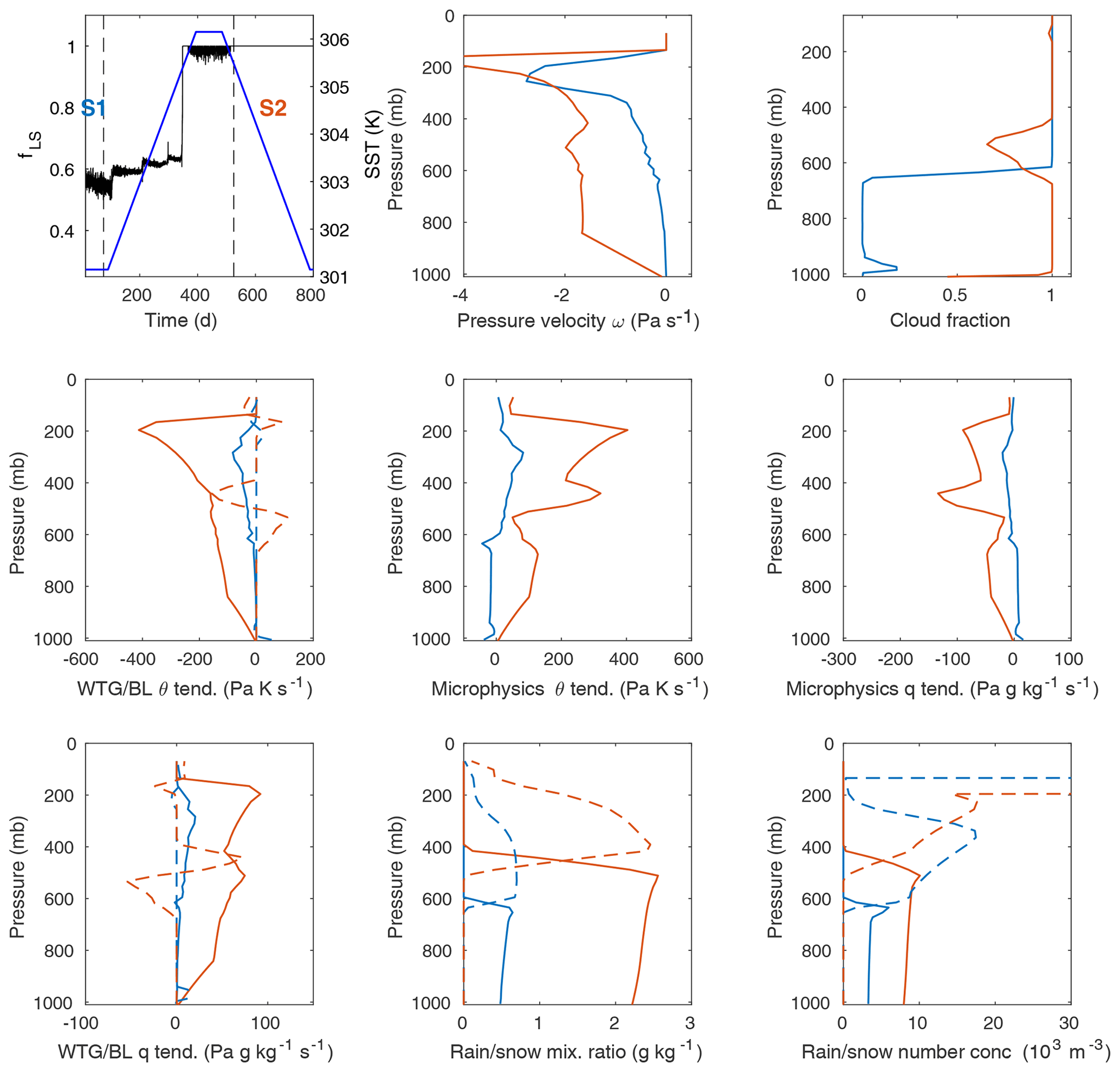
Figure 9 An experiment showing f_LS→1. The left axis of the top left plot shows f_LS for the WRF SCM over the heating phase of an 800 d integration with the WTG approximation active, a background profile calibrated for 301.15 K SST, and SST forcing from 301.15 K (28 ^∘C) to 305.15 K. A typical quasi-stationary state (S1, blue) and the f_LS=1 state (S2, red) are indicated. The right axis shows SST for the integration. The remaining plots show vertical profiles for the labeled quantities, averaged over time for each of the two states. In the WTG or boundary layer (BL) panels, solid lines show the WTG relaxation forcings, and dashed lines show the boundary layer forcings. In the plots for rain or snow mixing ratio and number concentration, solid lines represent rain, and the dashed lines represent snow. See also Table 4.

Table 4 Average values for various quantities for the S1 and S2 states from the f_LS→1 experiment shown in Fig. 9. After f_LS, the three types of precipitation (deep-convective P_D, large-scale P_LS, and shallow-convective P_SH) are shown, followed by the shortwave radiation to the surface (SWD), the outgoing longwave radiation from the ground (GLW), the outgoing longwave radiation at the top of the column (OLR), and the surface sensible (HFX) and latent (LH) heat fluxes.

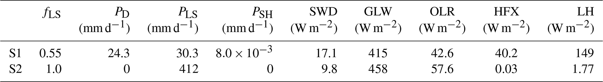
Figure 9 and Table 4 give average values for a number of variables for both a typical quasi-stationary state (S1) and the f_LS=1 state (S2) in an experiment showing the f_LS→1 transition just before the end of the SST increase. This experiment is identical to the experiment analyzed in Sect. 3.3, except that the SST forcing is from 301.15 K (28 ^∘C) to 306.15 K, and the WTG background profile is calibrated to SST 301.15 K.

Convective profiles are omitted from Fig. 9 as they are zero for the f_LS=1 state. Figure 9 also shows both the WTG relaxation forcings and the pure boundary layer forcings. Summed together, the cooling from the WTG and boundary layer θ and q forcings balance the heating from microphysics. The boundary layer–moist turbulence scheme acts higher in the column than usual, where it appears to play a role in mixing heat and moisture across the cloud base layer, similar in some ways to the function previously performed by the convective parameterizations.

As is evident from Table 4, convective rainfall not only ceases for f_LS=1, but the microphysics forcings and associated large-scale rainfall show dramatic increases, with forcings and rainfall rates an order of magnitude larger than those obtained for lower f_LS and as much as 2 or 3 orders of magnitude larger than the forcings and rates for a typical RCE experiment (see Fig. 2). Moreover, the balance of forcings in the column changes qualitatively again, with the WTG relaxation and boundary layer scheme now working together to balance microphysical heating (via melting or condensation) over the full depth of the column. Evaporation has now failed completely to cool the lower column and has switched over to warming.

4 Discussion

It seems clear that lower-column evaporative cooling plays an essential role in both initiating the abrupt transitions and keeping the column from falling into the f_LS→1 state. To better understand this, however, it is worth considering the overall balance of the column when the WTG approximation is active. We noted above that the magnitudes of the WRF SCM θ forcings are much larger in the WTG case than in the RCE case. This leads to a consideration of how the column stabilizes itself at the beginning of the WTG experiments, a close look at which suggests a positive heating feedback active (at first) in the upper column, which is ultimately balanced by a series of diabatic forcings (Fig. 10). Because heating in the upper column (whether coming from the convective or microphysics parameterizations) can only be balanced here by radiative cooling or the WTG relaxation – but more efficiently by the latter – heating at high levels generates an upward large-scale motion by Eq. (3), which then generates more heating due to condensation or freezing as water vapor is lifted into cooler air. The resulting cloudiness also blocks part of the outgoing infrared radiation from lower in the column, causing heating near the cloud base and causing the feedback to reach lower into the column. This feedback, which begins near the top of the column, causes upward motion lower and lower in the column until the falling precipitation reaches levels at which its melting or evaporation generates enough cooling to stop the feedback mechanism from reaching even lower into the column. Meanwhile, the large-scale rain resulting from this upper-column activity generates proportionally greater evaporative cooling below as the large-scale rain falls through the lower column, with this cooling balanced in turn by enhanced heating from the convective parameterizations. Finally, enhanced convection (especially coming from the shallow scheme) is able to deliver moisture and heat from the lower column to the layers around the cloud base, feeding the upper-column microphysics routine and thus allowing the balances depicted in Fig. 10 to hold for an overall warmer column.

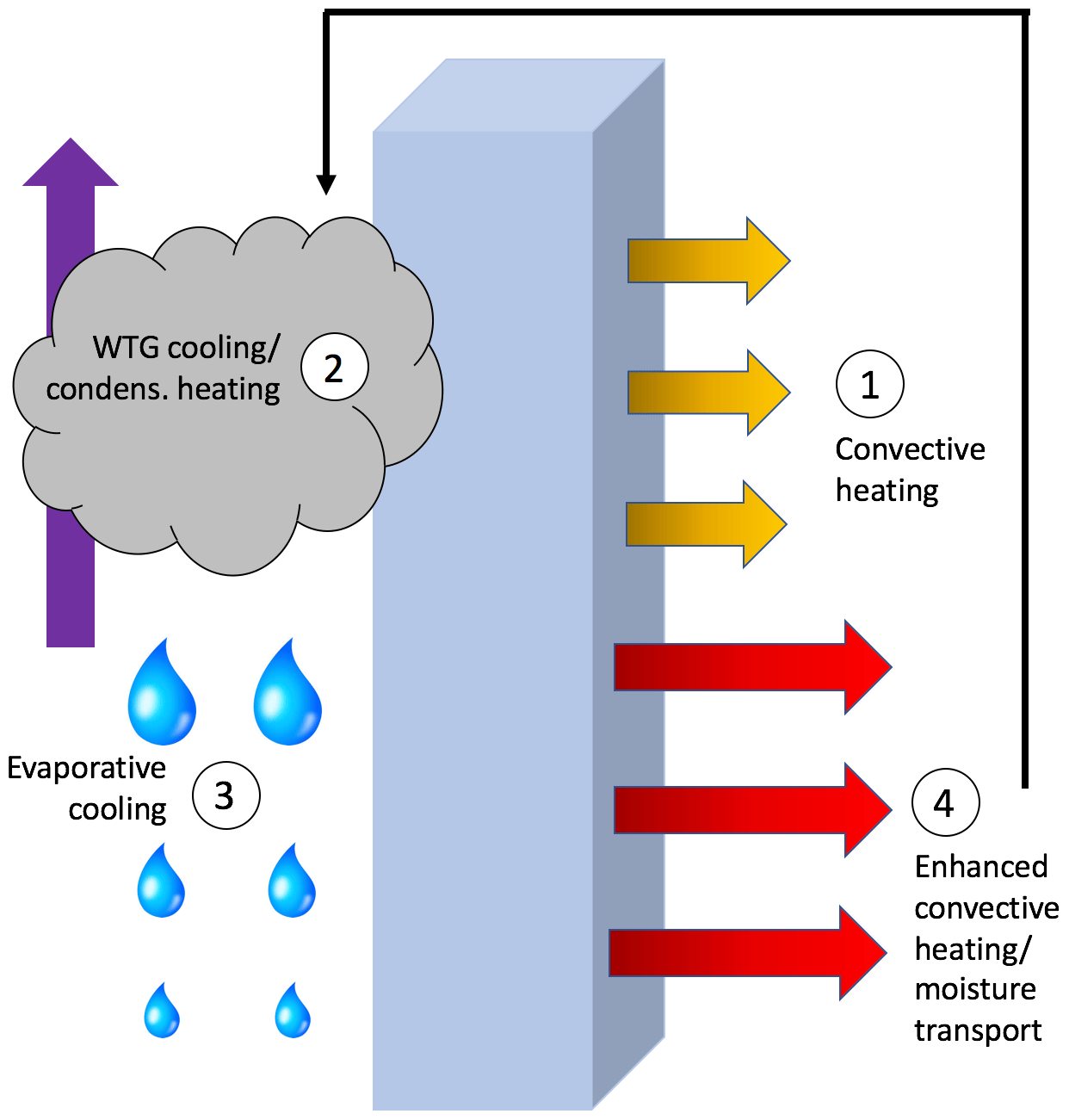
Figure 10 An illustration of the θ-forcing balances within the WRF SCM with WTG approximation and the order in which they appear to be established in the first few time steps. The 4→2 arrow signifies the convective parameterizations delivering moisture across the cloud base into the upper troposphere.

Some temperature forcings can respond quickly and without strong limits to temperature changes, while other forcings are limited such that the column equilibrium could become strained. The WTG relaxation simply adds or removes heat from the system (while inducing a vertical velocity) and has no inherent limitations. The shallow-convective parameterization too is unlimited in its vertical reach and precipitation rate; indeed, it can represent deep convection on its own if no deep-convective parameterization is employed (Park and Bretherton, 2009). It seems likely that this ability of the shallow scheme to work well beyond its “shallow” capacity is responsible for the proportionally greater increase in its heating role as SST increases (Fig. 5). On the other hand, the deep-convection scheme is limited by the CAPE-consumption timescale; it consumes CAPE at a rate proportional to the amount of CAPE (Zhang and McFarlane, 1995). Upper-column microphysical heating is limited by the availability of moisture there – if the convective routines and WTG lifting cannot deliver enough moisture, the condensational heating will not be maintained.

Similarly, lower-column evaporation is limited by the abundance of rainfall and its microphysical characteristics coming from above and by the local relative humidity. Because evaporative cooling provided to the lower column by the microphysics parameterization appears to be the first element of the Fig. 10 balance to fail as the system transitions to each new state – and because the lower-column heating closely follows the reduced evaporation – we attribute the transitions to nonlinearities within the microphysics routine.

The CAM microphysics routine is due to Hugh Morrison and various collaborators (Morrison et al., 2005; Morrison and Gettelman, 2008) and is based on diagnostic equations for the number concentration N and mixing ratio q of rain or snow droplets (but here the subscript “r” is for rain):

$$\begin{array}{}\text{(5)}& {\displaystyle }& {\displaystyle \frac{\mathrm{1}}{\mathit{\rho }}}{\displaystyle \frac{\partial }{\partial z}}\left(\mathit{\rho }{V}_{\mathrm{N}}{N}_{\mathrm{r}}\right)=-\sum _i{\left({\displaystyle \frac{\partial N_{\mathrm{r}}}{\partial t}}\right)}_i\text{(6)}& {\displaystyle }& {\displaystyle \frac{\mathrm{1}}{\mathit{\rho }}}{\displaystyle \frac{\partial }{\partial z}}\left(\mathit{\rho }{V}_q{q}_{\mathrm{r}}\right)=-\sum _i{\left({\displaystyle \frac{\partial q_{\mathrm{r}}}{\partial t}}\right)}_i,\end{array}$$

where V_N and V_q are the terminal fall speeds for rain (or snow) weighted by number and mass, respectively, and i indexes a number of terms due to various microphysical processes (condensation, melting, droplet growth by accretion or self-interaction, etc.), among which is evaporation of falling rain. Evaporation of rain in the CAM microphysics, of primary interest here, is given by

$$\begin{array}{}\text{(7)}& \begin{array}{rl}& P_{\mathrm{E}}=\\ & {\displaystyle \frac{\mathrm{2}\mathit{\pi }{N}_{\mathrm{0}}(S-\mathrm{1})\left[\mathrm{0.78}{\mathrm{\Lambda }}^{-\mathrm{2}}+\mathrm{0.32}{S}_{\mathrm{C}}^{\mathrm{1}/\mathrm{3}}{a}^{\mathrm{1}/\mathrm{2}}{\mathit{\nu }}^{-\mathrm{1}/\mathrm{2}}\mathrm{\Gamma }\left(\frac{b+\mathrm{5}}{\mathrm{2}}\right){\mathrm{\Lambda }}^{-(b+\mathrm{5})/\mathrm{2}}\right]}{\frac{L^{\mathrm{2}}}{K{R}_{\mathrm{v}}{T}^{\mathrm{2}}}+\frac{R_{\mathrm{v}}T}{e_{\mathrm{s}}{D}_{\mathrm{v}}}}}.\end{array}\end{array}$$

The numerator of Eq. (7) is related to the amount of available moisture, while the terms in the denominator account for evaporation's thermal and diffusive effects: N₀ and Λ are spectral parameters determining the raindrop size distribution (these are functions of N_r and q_r from Eqs. 5 and 6); a and b are empirically determined parameters giving the hydrometeor terminal fall velocity; $S\equiv e/e_{\mathrm{s}}$ is the ratio of ambient vapor pressure to saturation vapor pressure; ν is the kinematic viscosity; K and D_v are the thermal conductivity and mass diffusivity of water vapor in air, respectively; and $S_{\mathrm{C}}\equiv \mathit{\nu }/D_{\mathrm{v}}$ is the Schmidt number. (The thermal conductivity can be written as K=c_pρκ, where κ is the thermal diffusivity. In the WRF code, κ is replaced by the mass diffusivity D_v, acceptable for air–water vapor systems which have a Lewis number ($Le\equiv \mathit{\kappa }/D_{\mathrm{v}}$) of approximately 1.) The temperature and moisture dependence of Eq. (7) is quite complicated, with most of the variables determined by temperature and/or moisture.

As mentioned above, raw, high-resolution output taken from this equation during the WTG experiment confirms that the magnitude of P_E diminishes with each lower-column rolling temperature increase. Moreover, analysis of the individual terms of Eq. (7) indicates that the numerator is stable during the onset of the transitions, an expected result considering that the raindrop mixing ratio q_r and number density N_r – related to terms in the numerator – transition with the upper-column “snap” rather than with the lower-column “roll”. The saturation vapor pressure and thermal and diffusive terms, however, show rolling behavior alongside the temperature change, indicating that the local environment is more important in initiating the transition – that is, evaporation is not keeping pace with local heating.

The f_LS→1 behavior can be understood as a “runaway” case of the positive WTG heating feedback. If the only way in which the column can balance heating is via the WTG relaxation, this will generate additional heating above via lifting (and condensation) of moisture and heating below via absorption of infrared radiation at the newly generated cloud base. Indeed, a preliminary look at the θ forcings in several experiments showing the f_LS→1 transition reveals that near the transition, there is a point at which the evaporative cooling from the microphysics routine switches over into condensational heating. This means the deep- and shallow-convective routines and the microphysics parameterization are all working to heat the column at these levels; at this point, the only way the column can balance this heating is via radiative cooling or the WTG relaxation, the latter of which is again the more efficient. Hence the lower part of the column now experiences the WTG feedback, which spreads over the lower column, leading quickly to f_LS→1.

The extreme cloudiness shown by the WTG column, a consequence of using the realistic CAM radiation parameterization, would seem problematic. While cloud fractions can be fairly large in some areas of the tropics at high levels – for example, CALIPSO 2006–2014 data show cloud fractions as high as ∼0.8 for p<440 mb in the area of the Maritime Continent – the 100 % cloud cover consistently observed over the upper half of the WRF SCM column with the WTG approximation is unrealistic (although even higher fractions may be possible at smaller lengths and timescales). Prescribed radiative cooling seems to alleviate this problem (at least in the absence of anomalous SST forcing), keeping cloud fractions similar to their RCE values (which are also closer to observations), but this option is designed to isolate and study the interaction between convection and large-scale vertical advection. Since we are pursuing a different question involving the realistic case including cloud–radiation interactions, prescribed radiation is not an optimal solution. Furthermore, even with prescribed convection, SST forcing again generates the unrealistic 100 % cloud fractions in the upper column.

However, an intriguing possibility is that the high cloud and stratiform rainfall fractions can be interpreted in the context of mesoscale convective systems (MCSs). In a historical review of MCSs, Houze (2018) notes that mature MCSs typically show distinct convective and stratiform rainfall regions, with convective below and stratiform above, and – particularly in MCSs over the ocean – can have stratiform rainfall fractions as high as 70 %. The heating profile of such systems is top-heavy according to the amount of stratiform rain. These MCS features are consistent with the behavior of the WRF SCM under the WTG approximation, leading one to speculate whether the WTG approximation may emulate some behavior of mature MCSs under certain conditions. There are some discrepancies: the stratiform regions described by Houze (2018) are weakly buoyant, whereas those appearing in our simulations show intense upward motion.

As noted in the introduction, these transitions are a robust feature of the WRF SCM with CAM physics as long as the WTG approximation is implemented. Varying horizontal resolution has little effect on the transition behavior. Varying the WTG relaxation timescale τ has a more significant effect, with the f_LS→1 behavior more common and happening earlier for larger τ. Furthermore, we find broadly similar behavior with prescribed radiative cooling of −1.5 K d⁻¹ over the troposphere. The step-like transitions are not as common, and f_LS can show more oscillatory behavior, but the column can still transition to higher f_LS, and the f_LS→1 transition can still occur.

5 Conclusions

Using the WRF single-column model with CAM physics parameterizations and incorporating the weak temperature gradient approximation, we have found that abrupt transitions occur when SST is continuously increased, mimicking low-level convergence of sensible and latent heat. Beyond certain threshold temperatures, the column abruptly transitions to new configurations with larger fractions of large-scale (or nonconvective) rainfall. The stability of the column under WTG conditions appears to depend on delicate balances established between the various temperature and moisture forcings, and the SST-induced transitions appear to be initiated by a drop in the lower-column evaporative cooling coming from the microphysics parameterization. This breakdown can be traced to Eq. (7), which determines evaporative cooling; raw output from this equation suggests that the local temperature and moisture are more important than droplet number or mixing ratio in initiating the transitions.