the Creative Commons Attribution 4.0 License.
the Creative Commons Attribution 4.0 License.
 | 20 Oct 2020
Organization of convective ascents in a warm conveyor belt
Nicolas Blanchard
Florian Pantillon
Jean-Pierre Chaboureau
Julien Delanoë
Warm conveyor belts (WCBs) are warm, moist airstreams of extratropical cyclones leading to widespread clouds and heavy precipitation, where associated diabatic processes can influence midlatitude dynamics. Although WCBs are traditionally seen as continuous slantwise ascents, recent studies have emphasized the presence of embedded convection, the impact of which on large-scale dynamics is still debated. Here, detailed cloud and wind measurements obtained with airborne Doppler radar provide unique information on the WCB of the Stalactite cyclone on 2 October 2016 during the North Atlantic Waveguide and Downstream Impact Experiment. The measurements are complemented by a convection-permitting simulation, enabling online Lagrangian trajectories and 3-D objects clustering. Trajectories rising by 150 hPa during a relatively short 12 h window are identified as ascents and examined in the WCB region. One-third take an anticyclonic turn at upper levels, while two-thirds follow the cyclonic flow at lower levels. Identified trajectories that reach a 100 hPa (2 h)−1 threshold are further categorized as fast ascents. They represent one-third of the ascents and are located at lower levels mainly. Both radar observations and simulation reveal the presence of convective updrafts in the WCB region, which are characterized by moderate reflectivity values up to 20 dBZ. Fast ascents and updraft objects with vertical velocities above 0.3 m s−1 consistently show three main types of convection in the WCB region: (i) frontal convection along the surface cold front and the western edge of the low-level jet, (ii) banded convection at about 2 km altitude along the eastern edge of the low-level jet, and (iii) mid-level convection below the upper-level jet. Frontal and banded convection result in shallow ascents, while mid-level convection contributes to the anticyclonic WCB outflow. The results emphasize that convection embedded in WCBs occurs in a coherent and organized manner rather than as isolated cells.
- Article
(13955 KB) - Full-text XML
- BibTeX
- EndNote


Warm conveyor belts (WCBs) are large-scale, continuously poleward rising airstreams with significant cloud formation associated with extratropical cyclones (Harrold, 1973). They typically ascend by at least 600 hPa in 48 h (Wernli and Davies, 1997; Madonna et al., 2014) from the lower troposphere in front of the cyclone surface cold front and concentrate a wide range of cloud diabatic processes, leading to strong surface precipitation (Browning, 1999; Eckhardt et al., 2004; Flaounas et al., 2018).
During WCB ascent, latent heating from cloud diabatic processes modifies the structure of potential vorticity (PV) across the troposphere. Specifically, diabatic PV production (destruction) below (above) the heating maximum creates vertical PV dipoles within WCBs (Wernli and Davies, 1997; Joos and Wernli, 2012; Madonna et al., 2014). These diabatically generated PV dipoles can have an impact on flow evolution by strengthening the large-scale cyclonic (anticyclonic) circulation in the lower (upper) troposphere (Pomroy and Thorpe, 2000; Grams et al., 2011; Chagnon et al., 2013). The modification of PV within WCBs is mainly driven by latent heating resulting from condensation and water vapor deposition processes (Joos and Wernli, 2012; Chagnon et al., 2013; Martínez‐Alvarado et al., 2014; Joos and Forbes, 2016).
According to the classical WCB concept, cloud diabatic processes occur along large-scale slantwise airstreams with ascent rates that do not exceed 50 hPa h−1 (e.g., Browning, 1986). However, recent studies highlighted the occurrence of convective motions with faster ascent rates embedded in WCBs (Martínez‐Alvarado et al., 2014; Rasp et al., 2016; Oertel et al., 2019). These convective motions are mainly localized along the surface cold front (Martínez‐Alvarado et al., 2014; Rasp et al., 2016; Oertel et al., 2019). The associated diabatic heating is more intense than within slantwise WCBs ascents and induces the creation of mesoscale, horizontal PV dipoles with strong positive and negative values (Harvey et al., 2020; Oertel et al., 2020). In a North Atlantic case study, Harvey et al. (2020) suggested that PV dipoles occurring in multiple bands would be the natural result of parallel bands in heating in a larger-scale vertical wind shear environment. In a composite analysis, Oertel et al. (2020) showed that horizontal PV dipoles of a few tens of kilometers in diameter formed at the tropopause level above the center of convective updrafts embedded in a WCB. They suggested that convectively produced PV dipoles can merge to form elongated PV structures further downstream and locally accelerate the jet stream at the WCB outflow, thus impacting the upper-level dynamics.
Because of their impact on the large-scale flow, diabatic processes are considered a major source of model uncertainty at midlatitudes. Their representation influences the forecast skill of extratropical cyclones and high-impact weather downstream (Grams et al., 2011; Davies and Didone, 2013; Pantillon et al., 2013; Joos and Forbes, 2016). This motivated the North Atlantic Waveguide and Downstream Impact Experiment (NAWDEX; Schäfler et al., 2018), which took place from 19 September to 16 October 2016 with the use of many international facilities, including the deployment of four instrumented aircraft. The field campaign was specifically designed to investigate diabatic processes within WCBs and the evolution of large-scale flows in order to improve model forecasts over the North Atlantic and downstream over Europe.
This study is focused on the WCB of a cyclone known as the Stalactite cyclone (Schäfler et al., 2018) that occurred from 30 September to 3 October 2016 and was well observed during NAWDEX. Maddison et al. (2019) previously showed that the representation of the WCB of the Stalactite cyclone impacts the evolution of the downstream large-scale flow at upper levels. Here, detailed radar observations of this WCB are combined with a convection-permitting simulation over a large domain to investigate convective ascents and their organization and discuss their relationship with the mesoscale PV dipoles found in their vicinity.
The paper is organized as follows: Sect. 2 presents the radar observations made during the NAWDEX case study and describes the model simulation and analysis tools. Section 3 then details the identification of the large-scale cloud structure corresponding to the WCB and the Lagrangian trajectories that compose it, with a distinction between slow and fast ascents. Section 4 subsequently focuses on the characterization of the fast ascents that occur in the regions of observation, before generalizing the results to the entire WCB region. Section 5 discusses the impact of coherent convective ascents on the cyclone dynamics. Section 6 concludes the paper.
2.1 RASTA observations
RASTA (Radar Airborne System) is an airborne 95 GHz cloud radar (Delanoë et al., 2013). During the NAWDEX campaign, it was carried aboard the French Falcon 20 aircraft operated by SAFIRE (Service des Avions Français Instrumentés pour la Recherche en Environnement). RASTA measures both reflectivity and Doppler velocity along three antennas (nadir, backward and transverse) that allow for measuring three noncollinear Doppler velocities, from which the three wind components are reconstructed. The range resolution is 60 m with a maximum range of 15 km. The integration time is set to 250 ms for each antenna and leads to a temporal resolution of 750 ms between two consecutive nadir measurements. It corresponds to a 300 m horizontal resolution given a typical Falcon 20 speed of 200 m s−1. The minimum detectable reflectivity is approximately −35 dBZ at 1 km, depending on the antenna, with an accuracy of 1 to 2 dBZ (calibration is done using sea surface echo, Li et al., 2005; Ewald et al., 2019). On the afternoon of 2 October 2016, the aircraft flew over the WCB structure of the Stalactite cyclone (flight 7 of the Falcon 20 aircraft, Schäfler et al., 2018). Here we use the two legs that crossed the WCB between 14:48 and 15:18 UTC and between 15:21 and 16:02 UTC, hereinafter referred to as the 15:00 and 16:00 UTC legs, respectively (see the aircraft track in Fig. 1a).
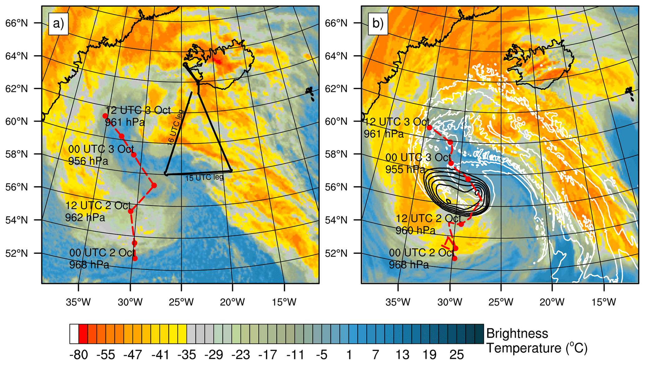
Figure 1The 10.8 µm brightness temperature (in ∘C) at 16:00 UTC (a) observed from MSG (raw data courtesy of EUMETSAT) and (b) simulated by Meso-NH. In panels (a) and (b), the cyclone track is shown (red dotted line, red mark every 6 h and MSLP minimum value every 12 h) for the ECMWF analysis and the Meso-NH simulation, respectively. In panel (a), the black line shows the track of the Falcon 20 aircraft and the 15:00 and 16:00 UTC legs. In panel (b), MSLP is shown with black contours every 1 hPa between 959 and 964 hPa and θe at 1 km altitude with white contours every 4 K between 300 and 316 K.
2.2 Meso-NH convection-permitting simulation
The nonhydrostatic mesoscale atmospheric Meso-NH model (Lac et al., 2018) version 5.3 is run over a domain of 2000 km × 2000 km covering the southeastern part of Greenland, Iceland, the Faroe Islands and the track of the Falcon 20 (Fig. 1). A horizontal grid mesh of 2.5 km is chosen allowing deep convection to be explicitly represented. The vertical grid has 51 levels up to 18 km with a grid spacing of 60 m in the first levels and about 600 m at high altitudes. The simulation uses the fifth-order weighted essentially non-oscillatory (WENO) advection scheme (Shu and Osher, 1988) for momentum variables and the piecewise parabolic method (PPM) advection scheme (Colella and Woodward, 1984) for the other variables. Turbulence is parameterized using a 1.5-order closure scheme (Cuxart et al., 2000), shallow convection with an eddy diffusivity mass flux scheme (Pergaud et al., 2009), microphysical processes in cloud with a single-moment bulk scheme (Pinty and Jabouille, 1998) and radiation with the European Centre for Medium-Range Weather Forecasts (ECMWF) code (Gregory et al., 2000). Fluxes exchanged between the surface and the atmosphere are represented by the Surface Externalisée (SURFEX) model (Masson et al., 2013).
The simulation starts at 00:00 UTC on 2 October 2016 when the Stalactite cyclone enters in the southwestern part of the domain and ends at 12:00 UTC on 3 October. Initial and boundary conditions are provided by 6-hourly ECMWF operational analyses with a horizontal resolution close to 9 km over the North Atlantic Ocean. To assess the simulated cloud fields, reflectivities and brightness temperatures (BTs) are calculated from the model hourly outputs and directly compared to the RASTA and Meteosat Second Generation satellite (MSG) observations, respectively. Synthetic reflectivities are computed using a version of the radar simulator developed by Richard et al. (2003) that has been modified to take into account gas absorption occurring at 95 GHz. Synthetic BTs are computed using the radiative transfer model for the TIROS Operational Vertical Sounder (RTTOV) code (Saunders et al., 2018), as done by Chaboureau et al. (2008) among many others. In the following, the results are shown for BT at 10.8 µm, which is mainly sensitive to the cloud top temperature.
2.3 Online trajectory calculation and clustering tools
Lagrangian trajectories are computed from three online passive tracers defined at each grid cell of the simulation domain (Gheusi and Stein, 2002). The tracers are initialized with their initial 3-D coordinates and are transported by PPM, a scheme with excellent mass-conservation properties and low numerical diffusion. Trajectories are analyzed during a 12 h window centered around the time of radar observations at 16:00 UTC. This time window is chosen to ensure that trajectories with high wind speed that cross the observation region at 16:00 UTC remain in the simulation domain. Increasing the time window quickly increases the number of incomplete trajectories, which strongly biases their general characteristics. Among the trajectories, ascents are defined as those for which the pressure decreases by at least 150 hPa in 12 h. This threshold is adapted for the 12 h duration of the trajectories from the usual WCB criterion of 600 hPa in 48 h (e.g., Madonna et al., 2014; Martínez‐Alvarado et al., 2014; Oertel et al., 2020). In contrast with previous studies, no condition is applied on the initial altitude of trajectories, which thus do not necessarily start in the boundary layer. Furthermore, the 150 hPa threshold does not ensure that selected trajectories perform a full ascent from the lower to the upper troposphere. The selected ascents are thus not all actual WCB trajectories but allow investigating upward motion that would otherwise be excluded with the usual criterion.
The clustering tool developed by Dauhut et al. (2016) is used to identify coherent structures. Here, updraft structures are defined as three-dimensional objects made of connected grid point for which the vertical velocity exceeds an arbitrary threshold. Two grid points sharing a common face, either horizontally or vertically, are considered connected, while diagonal connections are considered only vertically. No size criteria are applied. A threshold set to 0.3 m s−1 is found to identify the base of updraft structures well. This threshold is about 5 times higher than the typical ascent velocities of a WCB (around 10 km in 48 h, i.e., ≈0.06 m s−1). Similarly, negative PV structures are defined as regions of connected grid points with PV values less than −1 PVU (potential vorticity unit, 1 PVU=10−6 K kg−1 m2 s−1) and without any size criteria.
3.1 Cloud structures and track of the cyclone center
The observed BT in the simulation domain is shown at 16:00 UTC when the Stalactite cyclone was turning northeastward (Fig. 1a). A wide and elongated band of mainly high clouds (BT values less than −35 ∘C) indicates the WCB region in the southeastern quadrant of the domain. Mid-level clouds with BT values between −35 and 0 ∘C are also observed in the region. High clouds can also be distinguished close to Iceland further northwestward and suggest the outflow of the anticyclonic WCB branch (Martínez‐Alvarado et al., 2014). To the west, high and mid-level clouds wrap cyclonically around the cyclone center and illustrate the cloud head, which possibly merges with the cyclonic WCB branch. Between the WCB region and the cloud head, positive BT values locate the dry intrusion, whereas patches of negative BT values show the presence of isolated low-level clouds. The simulation correctly reproduces the main cloud structures (Fig. 1b), although with larger extent compared against MSG observations. As expected, the WCB region is characterized by high values of equivalent potential temperature (θe) at 1 km and is well covered by high and mid-level clouds. The cloudy region further northward, the cloud head and the dry intrusion are also well simulated.
The position of the mean sea level pressure (MSLP) minimum is shown along the 36 h duration of the simulation (dashed red line in Fig. 1). The MSLP minimum is tracked every 6 h within a radius of 250 km from its previous position in the ECMWF analysis and every 1 h within a radius of 160 km in the Meso-NH simulation. In the analysis, the Stalactite cyclone heads northward on the morning of 2 October, then jumps northeastward at 18:00 UTC and finally moves northwestward towards Greenland on 3 October. Thanks to hourly resolution, the simulated track reveals that the jump to the northeast is explained by the formation of a secondary MSLP minimum, as illustrated at 16:00 UTC in Fig. 1b. Overall, the simulation predicts the complete track from beginning to end well, including the jump and the deepening of the cyclone from 968 to about 955 hPa.
3.2 Identification of ascents
The location of air parcels fulfilling the ascent criterion of 150 hPa in 12 h is shown at 16:00 UTC as their spatial frequency (Fig. 2). It is integrated on all vertical levels and calculated on coarse meshes of 20 km × 20 km for better visibility. Surface fronts are identified with θe at 1 km altitude (colored contours). This reveals three high-frequency zones of ascending air parcels.

Figure 2Spatial frequency of air parcels belonging to identified ascents (shading) and θe at 1 km altitude (colored contours every 4 K between 288 and 312 K), all at 16:00 UTC. The black lines show the track of the Falcon 20 aircraft and the 15:00 and 16:00 UTC legs. The red box illustrates the mask used to focus on the WCB region.
The first zone is located between 56–64∘ N and 28–15∘ W above a region of homogeneous and relatively high θe. It corresponds to the WCB region overflown by the Falcon 20. Relatively high frequency of ascents is found in the core of this region, with local maxima identified in the middle of the 16:00 UTC leg and along the surface cold front. As expected, few or no ascents are detected in the dry intrusion, which is located upstream of the cold front and wraps around the pressure minimum. The red box in Fig. 2 is used as a mask to select the ascents in the WCB region at 16:00 UTC, which number more than 500 000 (out of nearly 3 million tropospheric trajectories contained in the red box, which means that about one-sixth are ascending). Thereafter, only these ascents are discussed.
The second zone is located in the western part of the simulation domain between approximately 54–64∘ N and 38–28∘ W. It corresponds to the cloud head, which wraps around the pressure minimum and is located above the bent-back front, marked by tight contours of θe. The third zone is located further north with two local maxima between 64–68∘ N and 40–25∘ W. The western maximum follows the Greenland coast, above the surface warm front of the Stalactite cyclone. Some of the ascents pass over the Greenlandic plateau (around 66∘ N between 40–35∘ W) and are likely due to a combination of warm frontal dynamics and the orographic forcing of Greenland. The eastern maximum is located between Greenland and Iceland around 66∘ N between 30 and 25∘ W, about 100 km behind the surface warm front. The origin of ascents in the second and the third zones is not addressed here, because the Falcon 20 did not fly over these zones at that time.
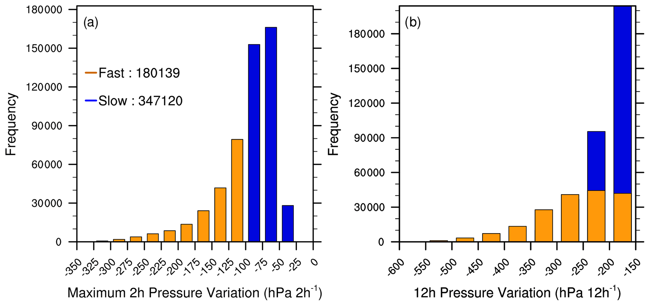
Figure 3Histograms of (a) maximum 2 h pressure variation (hPa 2 h−1) and of (b) 12 h pressure variation (hPa 12 h−1) along the selected ascents. Slow ascents are shown in blue and fast ascents in orange.
3.3 Distinction between slow and fast ascents
The properties of the more than 500 000 selected ascents are now examined. Following Rasp et al. (2016) and Oertel et al. (2019), trajectories are searched for short periods of enhanced upward motion. Figure 3a shows the frequency distribution of the maximum 2 h pressure variation along the trajectories from 11:00 to 21:00 UTC, a negative value of ΔP(2 h) corresponding to an upward motion. By construction, all trajectories underwent a maximum pressure variation stronger than 25 hPa in 2 h. This value corresponds to the typical slantwise ascent rate used for the identification of WCBs (i.e., 600 hPa in 48 h; Madonna et al., 2014). Two-thirds of trajectories underwent ascents between 25 and 100 hPa 2 h−1, i.e., 1 to 4 times the typical slantwise ascent rate. About 5 % of the trajectories reached ascent rates above 200 hPa 2 h−1 and some even 325 hPa 2 h−1 (<1 %). Such ascent rates have also been identified in recent studies combining convection-permitting simulation and online Lagrangian trajectories. Oertel et al. (2019) showed that 14 % and 3 % of the WCB trajectories identified in the NAWDEX cyclone Vladiana exceeded the ascent rates of 100 and 320 hPa in 2 h, respectively. Using a high ascent rate of 400 hPa in 2.5 h considered as convective, Rasp et al. (2016) found 55.5 % of trajectories meeting the threshold for an autumn storm over the Mediterranean Sea but none for a winter case over the North Atlantic. This shows that the proportion of fast ascents and their intensity varies a lot from case to case.
Hereafter, we define fast ascents as those reaching at least once a pressure variation greater than 100 hPa in 2 h between 10:00 and 22:00 UTC. The ascents that do not meet this criterion are defined as slow. This choice is motivated by the objective of determining the nature and characteristics of fast ascents. The specific value of the threshold has been set at a value equal to that used by Oertel et al. (2019) for comparison purposes. The use of another threshold would lead to a change in the proportion between slow and fast ascents. Thus, among the more than 500 000 trajectories, about one-third are categorized as fast ascents. Figure 3b shows that these fast ascents (in orange) had the strongest rise during the 12 h window, with about one hundred approaching 600 hPa in 12 h. However, most of them reached less than 300 hPa in 12 h. This suggests that strong upward motion occurs during a short period of time mainly, a typical feature of convection. In particular, fast ascents with a limited total rise likely encounter shallow convection, which will be discussed in the following section. In contrast, slow ascents (in blue) did not exceed a 250 hPa rise in 12 h and thus rather correspond to continuous slantwise motion.
3.4 Location of slow and fast ascents
An overview of the slow and fast ascents is given in Fig. 4. For the sake of visibility, only a sample of randomly selected trajectories is shown. At 10:00 UTC most slow ascents are located in the center of the region between 50–57∘ N and 20–15∘ W (red stars in Fig. 4a). A few isolated slow ascents are located further west, between 53–56∘ N and 23–20∘ W. Another group of slow ascents is located further north, between 57 and 60∘ N and between 25 and 20∘ W. At 16:00 UTC the slow ascents have moved with the large-scale flow and spread over the troposphere in the area overflown by the Falcon 20. Those located at an altitude z<8000 m (in blue, green and yellow) rise continuously and maintain a cyclonic turn until 22:00 UTC. They appear to wrap around the cyclone center and may belong to the cyclonic branch of the WCB, although WCB branches are typically considered at the outflow level (Martínez‐Alvarado et al., 2014). The slow ascents located higher in the troposphere (z>8000 m, in orange) take an anticyclonic turn and are located at higher latitudes (above 65∘ N) at 22:00 UTC and thus are likely part of the anticyclonic branch of the WCB.
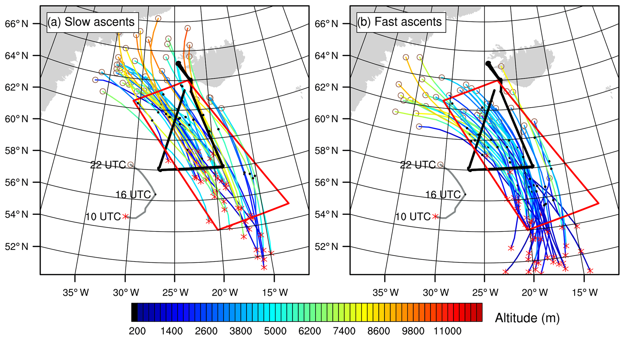
Figure 4Selected trajectories colored by altitude between 10:00 and 22:00 UTC for (a) slow ascents and (b) fast ascents. Only 40 trajectories are plotted for each category. Red crosses, black dots and brown circles show the location of the trajectories at 10:00, 16:00 and 22:00 UTC, respectively. The black lines show the track of the Falcon 20 aircraft, the grey curve the position of the MSLP minimum and the red box the region where the trajectories are selected at 16:00 UTC.
At first sight, Fig. 4b suggests that the fast ascents are colocated with the slow ascents. However, most fast ascents remain in the lower troposphere (z<4000 m, in navy blue) and keep a cyclonic turn during the 12 h window. Fast ascents in the middle troposphere ( m, in green and yellow) are advected further westward than those remaining in the lower troposphere. Only a few fast ascents, located in the upper troposphere (z>8000 m in orange), show an anticyclonic turn at 22:00 UTC. This suggests that the most elevated ascents, both slow and fast, are advected toward higher latitudes by the upper-level jet stream.
To distinguish the location of air parcels between slow and fast ascents, their spatial frequency is shown at 16:00 UTC for anticyclonic trajectories (Fig. 5a and b, respectively) and cyclonic trajectories (Fig. 5c and d, respectively). The distinction between cyclonic and anticyclonic trajectories is defined by their curvature during the last 2 h segment, i.e., between 20:00 and 22:00 UTC. With this definition, about one-third (two-thirds) of ascents are anticyclonic (cyclonic). While the slow and fast ascents partly overlap, along the cold front for instance, their location clearly differs depending on whether they take a cyclonic or anticyclonic turn.
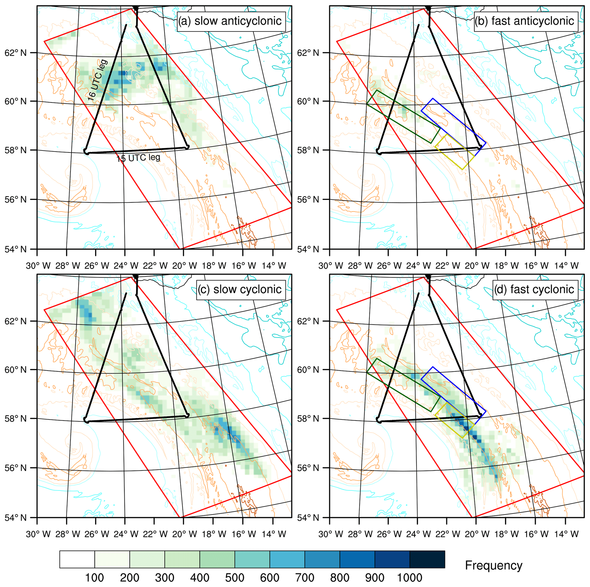
Figure 5As in Fig. 2 but for slow ascents with (a) anticyclonic and (b) cyclonic curvature and fast ascents with (c) anticyclonic and (d) cyclonic curvature zoomed on the region of selection (red box). In panels (b) and (d), the dark green, yellow and blue boxes are displayed for comparison with Fig. 10.
Slow ascents occur over much of the WCB region at 16:00 UTC (Fig. 5a and c). Most of slow ascents with anticyclonic trajectories are found between 60 and 62∘ N and between 28 and 20∘ W at that time (Fig. 5a). They account for two-fifths of the slow ascents. Slow ascents with cyclonic trajectories are located further northwest and southeast (Fig. 5c). They are mostly located in a region with relatively high and homogeneous values of θe at 1 km altitude, to the east of the dry intrusion. Hereafter, this region is defined as the core of the WCB. In contrast, few slow ascents are located along the western side of the WCB, near the surface cold front, and all show cyclonic trajectories. This contrasts with the case study of Martínez‐Alvarado et al. (2014), who found that the anticyclonic branch of the WCB originates from the cold front.
Fast ascent are mainly located along the surface cold front and more particularly in its southern part (Fig. 5b and d). This is consistent with the results obtained with a convection-permitting simulation by Oertel et al. (2019), who also found that the fastest ascents take place along the cold front and in its southernmost part especially. Here, most of the fast ascents take a cyclonic turn (Fig. 5d), whereas anticyclonic trajectories account for one-fifth of the fast ascents only (Fig. 5b).
3.5 Temporal evolution of the ascents
The temporal evolution of altitude and vertical velocity along the slow and fast ascents is shown in Fig. 6 between 10:00 and 22:00 UTC. These two categories are further subdivided between cyclonic and anticyclonic trajectories as explained in the previous subsection. To investigate the occurrence of convective motion, rapid segments are defined hereafter as the 2 h parts of ascents that rise by more than 100 hPa. They are further distinguished and shown separately depending on whether they belong to cyclonic or anticyclonic ascents. Note that, by definition, rapid segments can belong to fast ascents only.
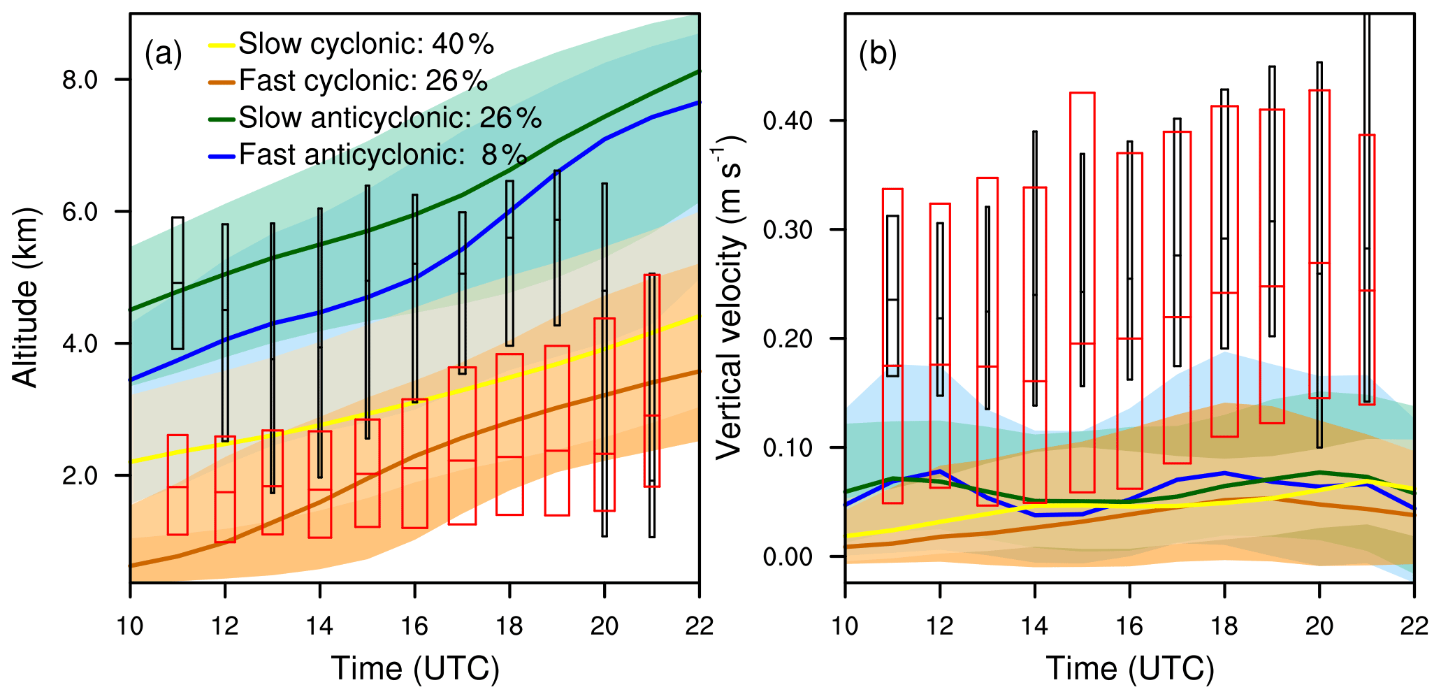
Figure 6Temporal evolution of (a) altitude (in km) and (b) vertical velocity (in m s−1) between 10:00 and 22:00 UTC. The median (colored bold curves) and the 25th–75th percentiles (shaded colors) are shown for slow cyclonic (yellow), fast cyclonic (red), slow anticyclonic (green) and fast anticyclonic (blue) ascents. The median and the 25th–75th percentiles for the 2 h rapid segments are shown with red and black boxplots for cyclonic and anticyclonic trajectories, respectively, with width proportional to their number.
All four categories of ascents exhibit a continuous rise during the 12 h window, as expected for WCB trajectories (Fig. 6a). On average, anticyclonic trajectories are located at higher altitudes than cyclonic trajectories. Anticyclonic ascents rise in the midtroposphere from z∼4 km at 10:00 UTC to z∼8 km at 22:00 UTC. Among them, fast ascents start ∼1 km lower on average, although the interquartile range shows a lot of overlap. Cyclonic ascents are concentrated in the lower troposphere between the surface and 2 km altitude at 10:00 UTC and rise to z∼4 km at 22:00 UTC. Fast cyclonic ascents also start ∼1 km lower than slow ascents on average but again with large overlap in the interquartile range. The fact that anticyclonic ascents are located higher than cyclonic ascents is consistent with the results of Martínez‐Alvarado et al. (2014) for WCB branches, although only anticyclonic trajectories reach typical altitudes of the WCB outflow here. The large overlap in altitude between fast and slow ascents suggests that convection is partly embedded in the slantwise flow, at least where their locations also overlap (e.g., near 58∘ N and 20∘ W in Fig. 5). While the altitude of trajectories clearly increases with time – by construction of the selection criterion – the altitude of rapid segments remains fairly stable with time, centered around 5 and 2 km along anticyclonic and cyclonic trajectories, respectively (black and red boxplots in Fig. 6a). Furthermore, their occurrence evolves but persists during the whole 12 h window (see width of the boxplots).
The vertical velocity signal is not as clear as the altitude signal (Fig. 6b). All four categories of ascents rise with vertical velocities below 0.1 m s−1 on average. Fast and slow ascents do not clearly contrast, which indicates that differences are diluted in the averaging process. In contrast, rapid segments reach vertical velocities of 0.2 m s−1 on average, which are greater along anticyclonic than cyclonic trajectories. As for their altitude, the vertical velocity of rapid segments remains fairly stable with time. This suggests that processes responsible for convective motion do not substantially change during the 12 h window.
Finally, and in contrast with results from Oertel et al. (2020), who found high graupel contents along convective trajectories, values largely remain below 0.1 g kg−1 here even in rapid segments (not shown). This is consistent with the relatively low values of vertical velocity.
This section focuses on the WCB region probed by the Falcon 20 aircraft along the 15:00 and 16:00 UTC legs. Observations, combined with simulation results, allow a more detailed characterization of the embedded fast ascents.
4.1 Mesoscale structures at 15:00 UTC
Infrared BT values obtained at 15:00 UTC from the MSG satellite show that the Falcon 20 flew westward from a band of high clouds into the dry intrusion and a few isolated low-level clouds below (Fig. 7a). These values are consistent with the vertical structure of reflectivity measured by RASTA (Fig. 7c). In the western part of the cross section, the dry intrusion is evidenced by reflectivities below −20 dBZ. Some isolated shallow clouds are actually located below 2 km altitude, below the dry intrusion. The most intense cell, with reflectivities greater than 15 dBZ suggesting a convective origin, extends over a 20 km width. Cirrus clouds indicated by reflectivities observed up to the aircraft altitude of 8.5 km are at the same location as BT values below −35 ∘C. Reflectivity values then increase below z∼7 km, except at the edges of the cloud. Local peaks up to 20 dBZ are measured at 2 km altitude. They indicate the melting level of frozen hydrometeors into liquid water. Peaks in reflectivity are of the same order of magnitude as observed previously in a WCB and associated with convection (e.g., Oertel et al., 2019). The horizontal wind speed measured by RASTA (black contours in Fig. 7c) allows us to approximately locate the jet stream above z∼5 km and the low-level jet around z∼1 km in the cloud structure.
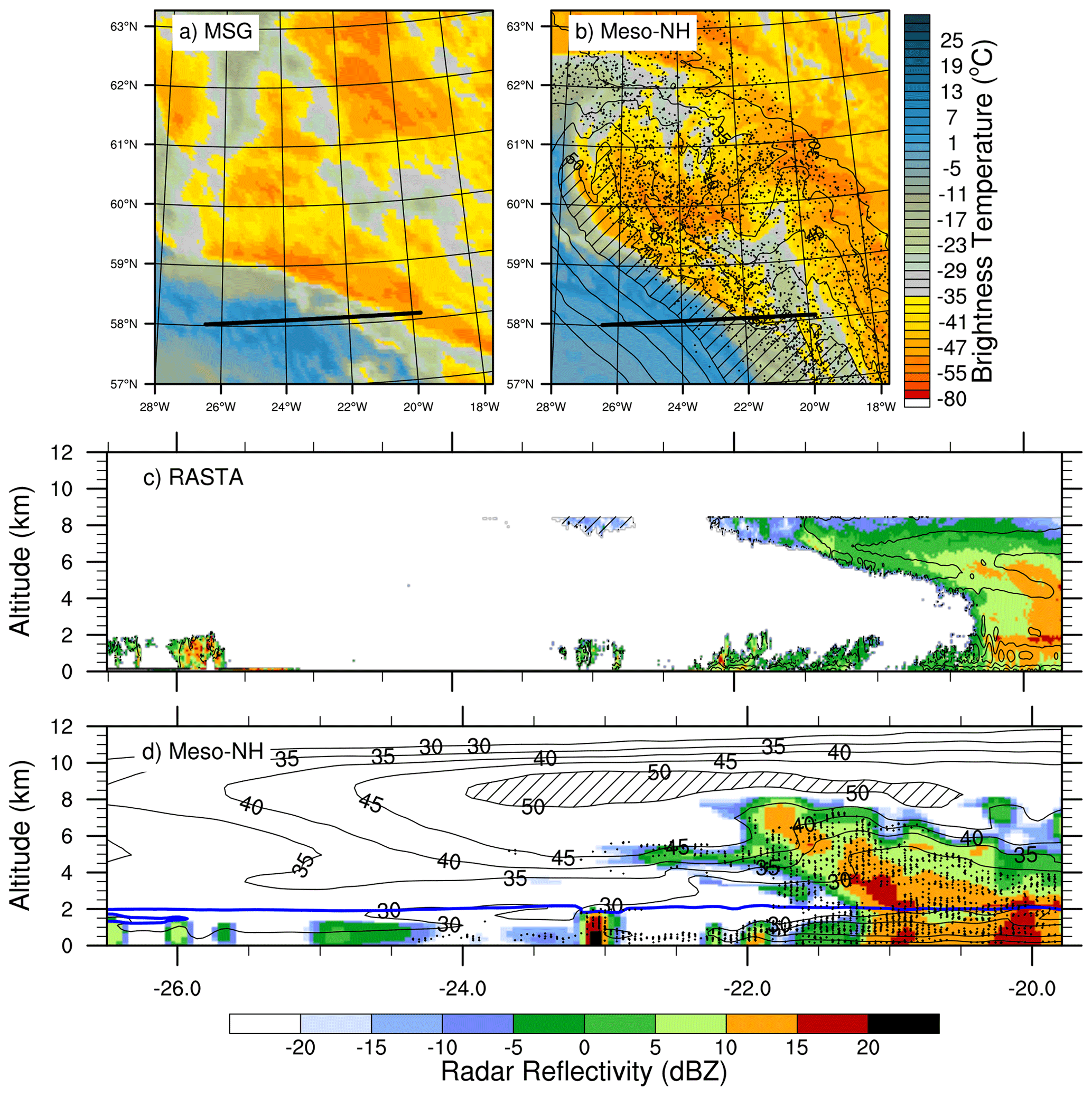
Figure 7Results at 15:00 UTC. (a, b) The 10.8 µm brightness temperature (in ∘C) (a) observed by MSG (raw data courtesy of EUMETSAT) and (b) simulated by Meso-NH. In panel (b), the black contours show the horizontal wind speed at 320 K with hatching for values greater than 50 m s−1. Central and bottom panels: reflectivity (in dBZ) (c) measured by RASTA and (d) simulated by Meso-NH along the black line shown in panels (a) and (b), respectively. The black contours show the horizontal wind speed (in m s−1) with hatching for values greater than 50 m s−1. In panels (b) and (d), the black dots indicate the position of the ascents (one trajectory every 60 in panel b). In panel (d), the blue contour shows the melting level.
The dry intrusion and the high cloud band are well reproduced by the simulation despite a more meridional inclination of the cloud band (Fig. 7b). The location, vertical extent and shape of the simulated cloud structure approximately correspond to the observations (Fig. 7d). Below the dry intrusion, an intense cell, with reflectivity values over 15 dBZ, extends over a 10 km width around 23∘ W. Another vertically developed, intense cell is simulated near 20∘ W. It extends above the melting level, which lies at about 2 km altitude. The jet stream core is located above the top of the clouds around z∼9 km between 24 and 20∘ W. The low-level jet extends from the surface up to z∼2 km over more than 2∘ of longitude. These horizontal wind structures correspond to those observed. The black dots show the location at 15:00 UTC of the selected ascents (fast and slow). Most of them are located in the cloud region, which thus corresponds well to the WCB. Some trajectories are located in isolated shallow clouds below the dry intrusion.
4.2 Fast ascents at 15:00 UTC
In addition to Lagrangian trajectories, fast ascents are identified as updraft objects using the clustering tool with a threshold set to w=0.3 m s−1. The base of the updraft objects, the horizontal wind speed and θe at 1 km altitude are shown in Fig. 8a. The wind speed emphasizes the low-level jet, which extends approximately between 57 and 61∘ N following the cyclonic flow in the lower troposphere. Four types of updrafts objects are identified. The first type is banded convection extending approximately between 58–60∘ N and 24–20∘ W along the eastern edge of the low-level jet core, with a base between 1 and 2 km altitude (in orange). The second type is mid-level convection that occurs above the western edge of the low-level jet (in blue and green). The third type is frontal convection that occurs along the western edge of the low-level jet, in its southern part mainly (in light orange). The fourth type consists of a few isolated shallow convective cells located to the west of the surface cold front (also in light orange). The location of rapid segments (black dots) is in agreement with these updraft objects. This shows that the (Eulerian) clustering and (Lagrangian) trajectory analyses used here consistently identify the fast ascents.
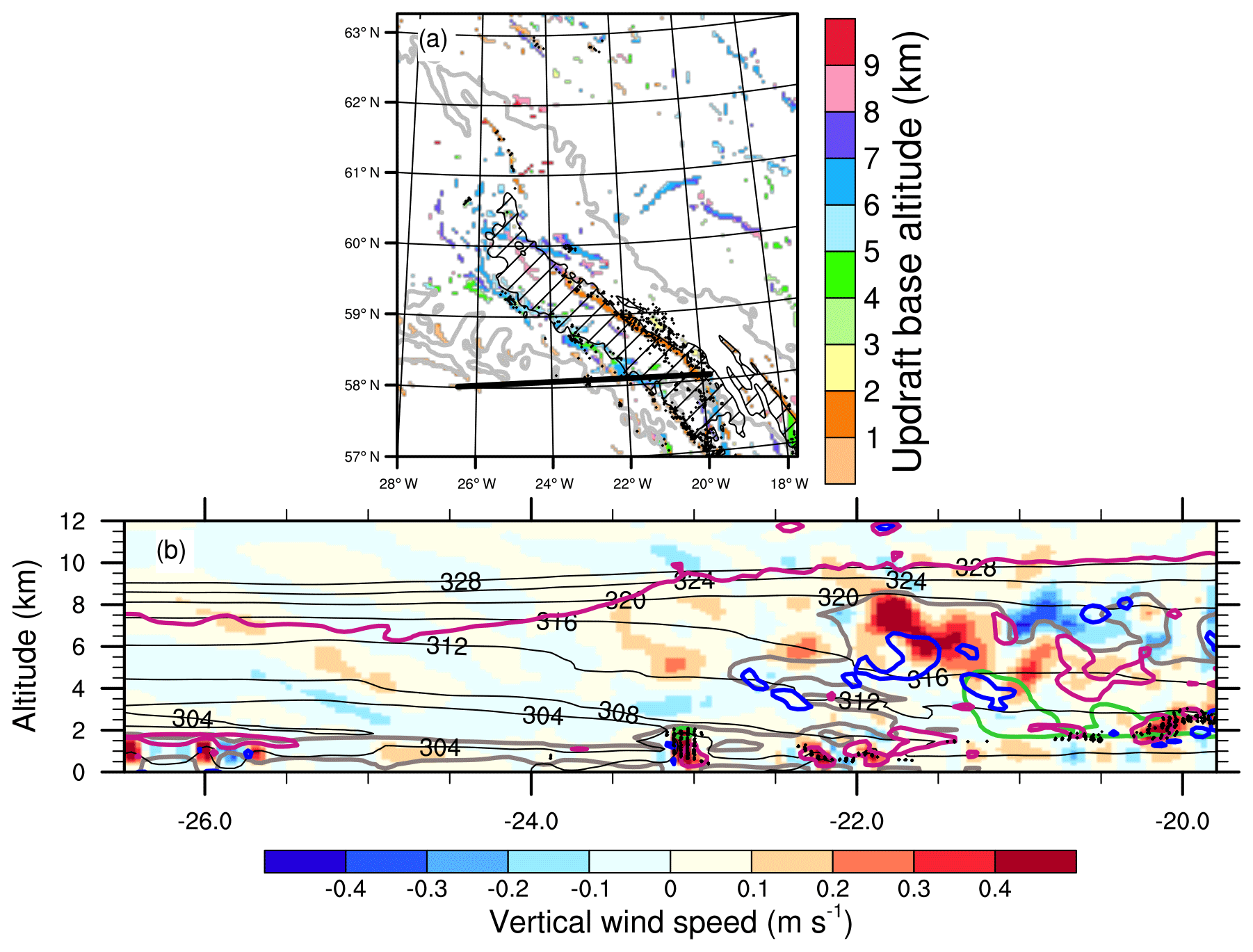
Figure 8Simulation results at 15:00 UTC. (a) Base altitude of the connected grid points with a vertical wind speed greater than 0.3 m s−1 (shading, km). Grey contours and hatching show equivalent potential temperature (from 305 to 320 K every 5 K) and horizontal wind speed (values greater than 35 m s−1) at 1 km altitude, respectively. (b) Vertical wind speed (shading, m s−1) and equivalent potential temperature θe (black contours, every 4 K) along the black line shown in panel (a). Grey and light green contours show the cloud and the graupel contents larger than 0.02 g kg−1, respectively. Magenta and navy blue contours show PV values equal to 2 and −1 PVU, respectively. In panels (a) and (b), the black dots indicate the position of the rapid segments (one trajectory every 10 in panel a).
Three of the four types of updrafts are found along the simulated 15:00 UTC leg, where convective motions are highlighted by relatively high vertical velocity values (w>0.3 m s−1, Fig. 8b). The westernmost cell around 23∘ W indicates isolated shallow convection, below z∼2 km and with cloud tops in the dry intrusion. Frontal convection is located at the western edge of the low-level jet around 22∘ W, also below z∼2 km. Banded convection is located between 2 and 3 km altitude in the core of the WCB, near 20∘ W. All three types are associated with regions of simulated reflectivity values greater than 15 dBZ (Fig. 7d). Banded convection also corresponds to a region with a relatively high graupel content larger than 0.02 g kg−1 (in light green in Fig. 8b). Other regions in the core of the WCB also have a relatively high graupel content, which is associated with a high reflectivity value and a high rain content below (not shown). However, these regions are not located in convective updrafts (w>0.3 m s−1). This suggests that the corresponding convective motions occurred upstream of the cross section before 15:00 UTC.
As in Fig. 8a, isolated shallow, frontal and banded convective structures correspond to the location of rapid segments in Fig. 8b (black dots). In contrast, this is not the case for high-level convective regions located between 5.5 and 8.5 km around 21.5∘ W. This discrepancy shows that the identification of fast ascents based on a pressure criterion focuses on lower levels, so that high vertical velocities at higher levels may not be identified as fast ascents (a value of 100 hPa 2 h−1 is equal to 0.12 m s−1 at the surface and 0.3 m s−1 at 300 hPa). Even higher, a 2 PVU contour (in magenta) locates the dynamical tropopause at z∼10 km east of 23∘ W in the vertical section. The PV contours also highlight the occurrence of positive and negative PV structures in the lower and midtroposphere.
4.3 Mesoscale structures at 16:00 UTC
During the 16:00 UTC leg, the Falcon 20 aircraft left the dry intrusion and flew over the WCB region further north (Fig. 9a). In particular, it overflew part of the band of high cloud between 60 and 63∘ N. A vertical section of reflectivity measured by RASTA along this leg provides more details on the internal structure of the WCB clouds (Fig. 9c). Reflectivity values around z∼8 km correspond to the presence of the high clouds observed by MSG. Under these high clouds, the higher positive reflectivity values show the presence of low and middle layer clouds. Peaks up to 20 dBZ suggest the presence of convection in the middle troposphere. Below, the bright band again emphasizes that the melting level is localized around z∼2 km. Some low and middle layer clouds are located further west, at the edge of the WCB and into the dry intrusion. There, convection forms narrow, vertically extended structures of reflectivity values above 10 dBZ. Their width is between 10 and 20 km and their height is about 2 km. Horizontal wind speed values above 40 m s−1 indicate that the jet stream extends between z∼5 km from the dry intrusion to z∼8 km within the WCB. The jet stream core is not visible in radar imagery because it does not contain clouds. In contrast, the low-level jet is clearly seen and characterized by horizontal wind speed values greater than 30 m s−1. It extends horizontally for more than 500 km and vertically between the surface and z∼2 km inside the cloud structure.
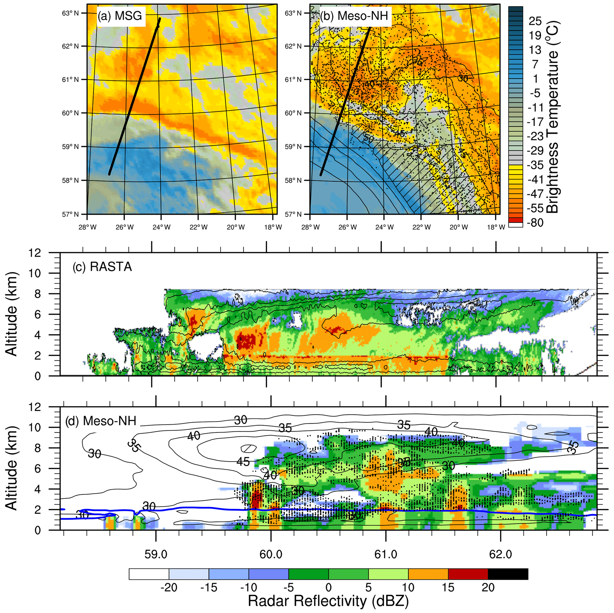
Figure 9As in Fig. 7 but at 16:00 UTC.
As at 15:00 UTC, the dry intrusion and cloud structures observed by MSG at 16:00 UTC are well reproduced by the model (Fig. 9b). Once again, the large majority of ascents issued from the trajectory analysis corresponds to the cloud areas. The vertical section of radar reflectivity is also fairly well reproduced by the model, although the horizontal extent of the clouds is more limited in the simulation (Fig. 9d). Around 60∘ N, two narrow, vertically extended cells of reflectivity values above 10 dBZ mimic the observation with similar width and height. The bright band is less defined than in the observation, suggesting too little simulated melting of snow into rain. Compared to 15:00 UTC, both clouds and ascents reach higher altitudes (up to z∼10 km). As for the simulated jet stream, it is less extended above the cloud structure than at 15:00 UTC. Its core is smaller and located at the western edge of the WCB, which is consistent with the higher cloud tops (compare Figs. 7d and 9d). Finally, the intensity and horizontal extent of the simulated low-level jet at 16:00 UTC correspond to those measured by the Falcon 20.
4.4 Fast ascents at 16:00 UTC
The convective objects described at 15:00 UTC are advected northwestward at 16:00 UTC by the large-scale cyclonic flow (Fig. 10a). Banded convection is still located along the eastern edge of the low-level jet. Between 15:00 and 16:00 UTC, more mid-level convective cells formed above the northwestern edge of the low-level jet. Frontal convection is still located along the southwestern edge of the low-level jet and the cold front, while isolated shallow convective cells are found further southwestward. A vertical cross section along the 16:00 UTC leg largely misses convective structures in the simulation (not shown). Its position is therefore shifted 0.5∘ westward to better capture convective structures close to the WCB areas overflown by the Falcon 20.
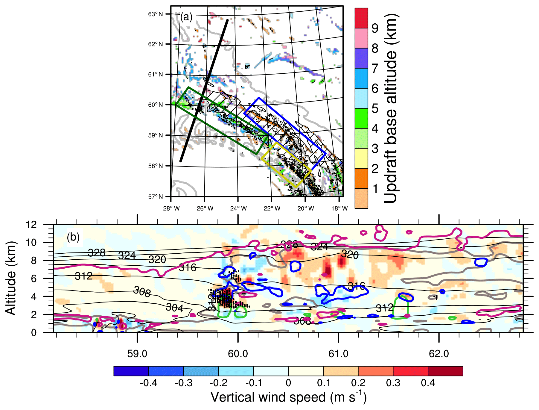
Figure 10As in Fig. 8 but at 16:00 UTC. In panel (a), the dark green, yellow and blue boxes show where the three categories of fast ascents have been selected (see text).
As for 15:00 UTC, simulated convective structures are highlighted by vertical velocity values greater than 0.3 m s−1 at 16:00 UTC (Fig. 10b). A mid-level convective cell is identified near the western edge of the WCB, around 60∘ N. It extends between km and resembles the convective cloud at the western edge of the WCB, where reflectivity values greater than 15 dBZ were measured by RASTA (Fig. 9c). Positive and negative PV structures are present around the cell, which reminds of the horizontal PV dipoles centered around composites of convection embedded in WCB found by Oertel et al. (2020). Three other convective cells are identified above 6 km and up to 9 km altitude in the core of the WCB, around 60.5∘ N in the vertical section. Once again, because of the identification of fast ascents based on a pressure criterion, these high-level isolated convective structures are not colocated with rapid segments (black dots) and thus not further discussed here.
4.5 Generalization to all identified updraft objects
Results obtained from the study of updraft objects identified in Figs. 8b and 10b are generalized to all updraft objects located in the vicinity of observations at 16:00 UTC. Three main regions of organized convection are selected (Fig. 10a). The first region (in blue) covers much of the eastern edge of the low-level jet, where banded convection occurs. The second region (in dark green) covers the northwestern part of the low-level jet core, where mid-level convection takes place. The third region (in yellow) covers the southwestern part of the low-level jet, where frontal convection is found. Note that the three regions largely encompass the rapid segments occurring at 16:00 UTC. The isolated shallow convective cells identified before are partly included in the frontal convection region but do not significantly contribute and are too rare to constitute an extra category.
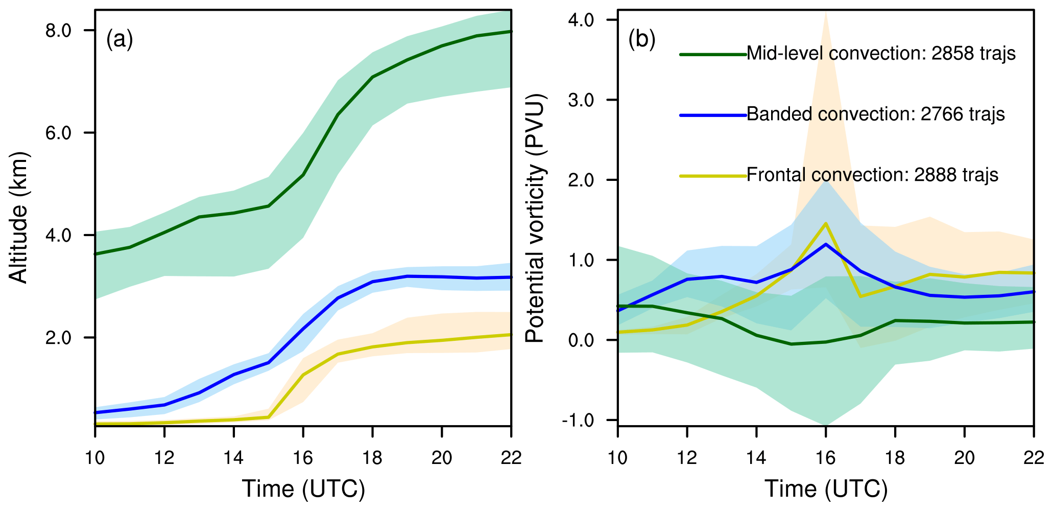
The three selected regions contain about the same number of rapid segments (∼2800). Time evolutions of altitude and PV are shown in Fig. 11 along the corresponding trajectories associated with each region. The altitude (Fig. 11a) confirms the location of the three convection categories at 16:00 UTC. All categories show consistent evolution with small interquartile range and are thus relevant. Banded convection (in blue) and frontal convection (in yellow) originate in the lower troposphere at 10:00 UTC. The banded convective trajectories slowly ascend the lower layers of the troposphere and are located at z∼1.5 km on average at 15:00 UTC, while the frontal convective trajectories have not started their ascent yet. Both categories finally undergo a rapid rise between 15:00 and 17:00 UTC and reach higher altitudes (z∼3 km and z∼2 km on average for the banded convective cells and the frontal convective cells, respectively) before stabilizing in the lower troposphere until 22:00 UTC. The mid-level convective trajectories are already located at km on average at 10:00 UTC and rise to 7–8 km of altitude on average at 22:00 UTC. These results suggest that trajectories associated with banded and frontal convection at lower levels encounter shallow convection rather than actual WCB ascent. In contrast, trajectories associated with mid-level convection reach typical heights of WCB outflow and thus likely belong to full tropospheric ascents.
Time evolutions of PV for the banded and frontal convection show positive peaks between 1 and 1.5 PVU on average at 16:00 UTC during the quick rise (in blue and yellow in Fig. 11b). The third quartile indicates PV values greater than 4 PVU in the frontal convective regions. This demonstrates that PV is created in these two convective regions. In contrast, the time evolution of PV for the mid-level convection shows a decrease until 16:00 UTC, when its average reaches zero and the first quartile even shows a negative peak below −1 PVU (in green). This differs from the evolution at low levels, which matches the typical increase below the heating maximum and decrease above (Wernli and Davies, 1997). Instead, the evolution at mid-levels is similar to that shown by Oertel et al. (2020) (see their Fig. 12), who found trajectories that acquire a negative PV value when they pass to the left of a convective updraft region.
Finally, the path followed by trajectories associated with the three selected regions is shown between 10:00 and 22:00 UTC (Fig. 12). For the sake of visibility, only a small sample of trajectories is plotted. Banded convection shows trajectories that remain coherent over time and is followed by frontal convection trajectories that turn northward around 14:00 UTC. Mid-level convection trajectories remain localized further westward with increasing separation from the other categories during the 12 h window. Banded and frontal convection trajectories follow a cyclonic path and are therefore part of the 26 % of cyclonic fast ascents. In contrast, the mid-level convection category is split between a majority of anticyclonic trajectories, which thus belong to the 8 % of anticyclonic fast ascents, and a minority of cyclonic trajectories. The bifurcation between these trajectories depends on altitude; the lower ones keeping a cyclonic curvature until the end of the time window. The fact that both anticyclonic and cyclonic mid-level convection trajectories are located along the western edge of the WCB at 16:00 UTC is consistent with the overlap of the fast anticyclonic and cyclonic ascents at that time (see green box in Fig. 5b and d). Similarly, the location of banded and frontal convection in the WCB core at 16:00 UTC is consistent with the location of fast cyclonic ascents at that time (blue and yellow boxes).
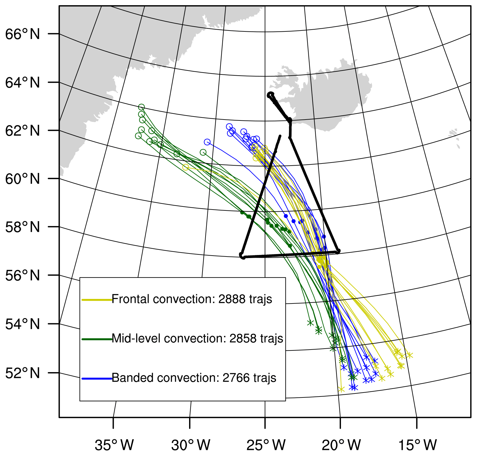
Figure 12Trajectories of banded (in blue), frontal (in yellow) and mid-level (in green) convection between 10:00 and 22:00 UTC. Crosses, dots and circles show the location of the trajectories at 10:00, 16:00 and 22:00 UTC. Only 10 samples are shown in each category.
This section discusses the possible impact of convective ascents on mesoscale dynamics, inspired by recent studies that have highlighted the presence of mesoscale upper-level negative PV structures close to the jet stream core (Oertel et al., 2020; Harvey et al., 2020). The clustering approach previously used to identify updraft objects is applied here to follow the evolution of mid-level and upper-level negative PV structures, which potentially influence the jet stream and large-scale dynamics. Hereafter, negative PV structures are defined as regions with PV values less than −1 PVU in order to obtain coherent PV regions that are straightforward to interpret. The top altitude of such structures is shown in close-ups following their advection to the northwest at 11:00, 16:00 and 21:00 UTC (Fig. 13a, c and e, respectively). The upper-level wind is overlaid and thus allows a comparison between the location of the negative PV structures and the jet stream. To complete the analysis, the rapid segments occurring at the indicated times are represented by black dots. This makes it possible to discuss the occurrence of the fast ascents embedded in the WCB between 11:00 and 21:00 UTC, thus assessing whether the convective structures characterized at 15:00 and 16:00 UTC are representative of the period studied. Modifications of the PV field in the convective regions are further investigated in vertical sections (Fig. 13b, d and f) selected to cross both rapid segment regions (black dots) and negative PV structures (blue shading) at 11:00, 16:00 and 21:00 UTC (see their locations in Fig. 13a, c and e).
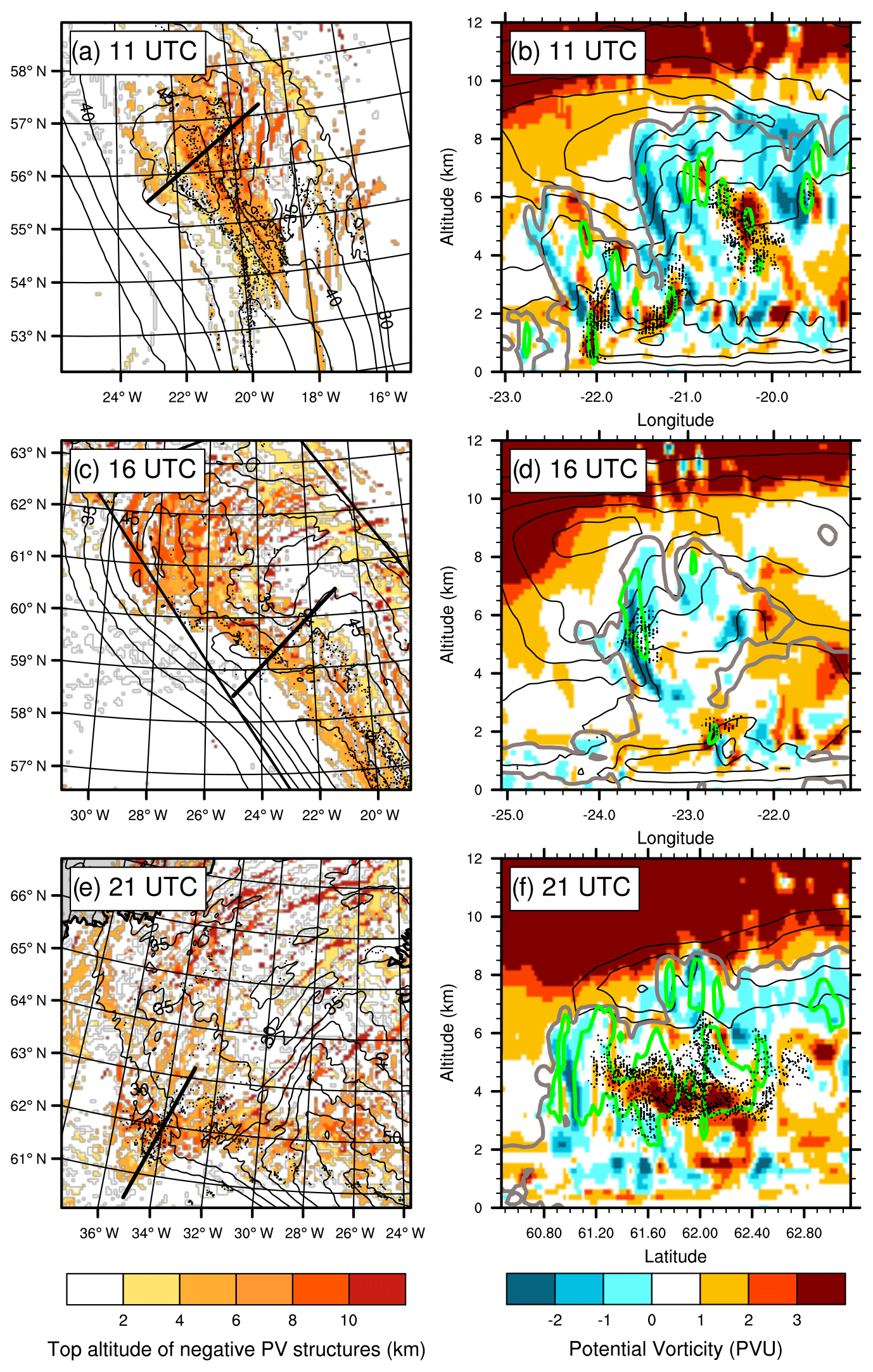
Figure 13PV at (a, b) 11:00 UTC, (c, d) 16:00 UTC and (e, f) 21:00 UTC in (a, c, e) maps of the top altitude of identified clusters below −1 PVU (shading, km) and (b, d, f) vertical cross sections along the black thick line shown in panels (a), (c) and (e), respectively. Dots indicate the position of rapid segments. Black contours show horizontal wind speed (a, c, e) at ∼9 km and (b, d, f) in the cross sections (values larger than 30 m s−1 every 5 m s−1). In panels (b), (d) and (f) green contours show the vertical velocity equal to 0.3 m s−1.
At 11:00 UTC, the location of rapid segments is consistent with that of coherent upper-level negative PV structures (above z=5 km), which extend meridionally and follow the eastern side of the jet stream core (Fig. 13a). Frontal and banded convection, previously identified at 16:00 UTC (see Sect. 4.5), are already present at that time (Fig. 13b). As in Fig. 8, frontal convection is located to the west of the low-level jet core (at 22∘ W, below 2 km altitude in Fig. 13b), while banded convection is located above the low-level jet core (at z∼2 km around 21.2∘ W). Mid-level convection is also identified in the WCB between km around 20.2∘ W. These convective regions are associated with regions of vertical velocity w>0.3 m s−1 (green contours) and PV values larger than 3 PVU. This suggests that PV is produced by convection in these regions. In addition, negative PV structures are widespread in the WCB. They remain generally shallow (vertical extent <1 km), especially in lower layers at z∼2 km, while they extend further vertically in the upper troposphere. In particular, a negative PV tower is located at the western cloudy edge of the WCB and just below the core of the jet stream (around 21.5∘ W between km in Fig. 13b).
At 16:00 UTC, the upper-level negative PV structures extend and rise in altitude following the head of the jet stream, where the maximum horizontal wind speeds are located (Fig. 13c). Negative PV structures take the form of elongated bands and are curved anticyclonically. They continue to extend away from each other in the head of the jet stream. They are partly overflown by the Falcon 20 at 16:00 UTC (compare with Fig. 10a). A negative PV tower is still located at the western edge of the WCB, between km around 23.5∘ W (Fig. 13d). At that time, it clearly corresponds to a mid-level convective region that is characterized by both updrafts (w>0.3 m s−1) and rapid segments (black dots). Banded convection is captured further east above the low-level jet and is less extended vertically than at 11:00 UTC. Frontal convection does not appear in the vertical section because it is located further south (see Fig. 13c).
At 21:00 UTC, the elongated negative PV bands eventually thin out and disperse while the head of the jet stream disappears (Fig. 13e). Only mid-level convection still occurs on the western edge of the head of the jet stream at 21:00 UTC. Mid-level convective cells detach from the low-level jet and the core of the jet stream between 16:00 and 21:00 UTC and extend further vertically (Fig. 13f). Those located in the core of the WCB are associated with regions of rapid segments with high positive PV values, between km and 62.8–61.2∘ N, while a negative PV tower is again present at the western edge of the WCB, between km and 60.8–61.2∘ N (Fig. 13f). Altogether, the clustering approach shows that elongated negative PV bands persist for several hours and are mainly found near the head of the jet stream, which is the region where mid-level convection also takes place.
This study focuses on the occurrence of convective ascents within the WCB of the Stalactite cyclone that approached Iceland on 2 October 2016. For this purpose, detailed RASTA radar observations of the WCB cloud structure carried out during the NAWDEX field campaign are combined with a Meso-NH convection-permitting simulation covering the mature phase of the cyclone. The simulated cloud structures are in good spatial and temporal agreement with satellite observations on the large scale and radar observations on the kilometer scale, while the trajectory of the simulated cyclone is also consistent with the ECMWF analysis.
Online Lagrangian trajectories are followed during a 12 h window centered around the time of the radar observations. Trajectories rising by 150 hPa in 12 h are defined as ascents, based on the usual WCB pressure criterion of 600 hPa (48 h)−1 (e.g., Madonna et al., 2014) and adapted to the shorter time window and without constraint on the initial or final height. Ascents satisfying the selection criterion are identified in three regions with high clouds: the WCB region, characterized by high values of θe; the cloud head, which wraps around the cyclone center and follows the bent-back front; and a third zone above the surface warm front and with orographic forcing from the Greenland plateau. The focus here is on the WCB region, where aircraft observations took place.
Following Rasp et al. (2016) and Oertel et al. (2019), fast ascents are further distinguished from slow ascents by applying an additional pressure threshold set to 100 hPa in 2 h here. This results in one-third of fast ascents, with ascent rates between 100 and 325 hPa in 2 h, among the ∼500 000 selected trajectories. Fast ascents are concentrated on the western edge of the WCB, close to the surface cold front, while slow ascents are rather distributed on the eastern edge. This is consistent with the results of Oertel et al. (2019) for the NAWDEX case study of cyclone Vladiana. While two-thirds of ascents – both fast and slow – follow the large-scale cyclonic flow between 10:00 and 22:00 UTC, one-third take an anticyclonic curvature when their outflow joins the jet stream at the end of the time window. Anticyclonic ascents are located higher than cyclonic ascents and reach typical altitudes of the WCB outflow, thus resembling the anticyclonic WCB branch (Martínez‐Alvarado et al., 2014). However, contrary to the findings of Martínez‐Alvarado et al. (2014), anticyclonic trajectories originate from the WCB head rather than from the cold front. Finally, during their rise, the ascents undergo a vertical motion of the order of 0.1 m s−1 associated with the production of low graupel contents on average during the 12 h window. Higher values are reached by rapid segments, which are most often located in the lower troposphere. However, these values remain lower than those of convective WCB ascents in Oertel et al. (2019), suggesting case-to-case variability.
Radar observations reveal structures of high reflectivity in the lower, middle and upper troposphere, thus providing evidence for the existence of fast ascents. These structures are correctly reproduced by the Meso-NH simulation – as is the bright band near z=2 km – where they are associated with rapid segments and vertical velocity larger than 0.3 m s−1. These characteristics suggest that the identified fast ascents are actually convective cells embedded in the WCB. The observed mesoscale dynamics are also correctly reproduced in the simulation. A clustering analysis based on the identification of coherent 3-D updraft objects highlights three main types of organized convection at the time of observations. The first type is located at the southwestern edge of the WCB and coincides with the western edge of the low-level jet. It is named “frontal convection” because of its proximity with the surface cold front, and matches early observations by Browning and Pardoe (1973). The second type is located above and to the east of the core of the low-level jet and is named “banded convection” because it forms a long band that extends over several hundreds of kilometers. The third type is located along the western edge of the WCB below the upper-level jet. It is named “mid-level convection” due to its higher altitude.
The trajectories participating in frontal and banded convection come from the boundary layer and remain below 3 km altitude. Their geographical path indicates that they are advected by the cyclonic flow during the whole 12 h study period. In contrast, the trajectories participating in mid-level convection start above 3 km and rise up to 8 km altitude. They take an anticyclonic curvature mostly. Frontal and banded convection trajectories thus resemble shallow convective ascents that do not clearly belong to the WCB, while mid-level convection trajectories appear to be part of the WCB outflow. The time evolution of PV shows that frontal and banded convection undergo a short but strong PV gain during ascent, while mid-level convection encounters a decrease in PV at the time of rapid ascent. Negative values are found along half of the mid-level convection trajectories, suggesting that they are associated with negative PV creation. The former corresponds to the classical view of the vertical PV dipole within WCBs described by Wernli and Davies (1997), while the latter contradicts the classical view but agrees with recent results obtained from mesoscale simulations and observations (Oertel et al., 2020; Harvey et al., 2020).
Identifying the main convective regions near the beginning and end of the 12 h window reveals that the three types of convection found at the time of the observations are representative of the convective motion embedded within the WCB during the whole study period. Furthermore, the clustering analysis highlights the presence of upper-level structures of negative PV in the regions of organized convection. These structures extend horizontally to form elongated bands with anticyclonic curvature, especially at the eastern edge of the jet stream head. They also extend vertically to form negative PV towers in the WCB, under the jet stream in particular. The elongated negative PV bands persist for several hours before dispersing, as do the convective regions and the jet stream head. The common shape, location and timing between the identified structures and rapid segments suggest that the organization of negative PV bands may be related to the organization of convection. The organized nature of convection in WCBs may thus explain the merging of isolated PV dipoles into coherent structures, whose role in mesoscale dynamics is currently being debated (Oertel et al., 2020; Harvey et al., 2020). However, mid-level convective ascents alternatively coincide with positive and negative PV structures, depending on the considered time. Unlike the composite study of Oertel et al. (2020), the formation of horizontal PV dipoles around convective cells thus does not appear systematic, which calls for a more thorough investigation of negative PV formation within WCBs.
Overall, this study suggests that convection in WCBs mainly consists in coherent and organized convective structures that persist with time rather than isolated convective cells embedded in the large-scale slantwise ascent. Furthermore, mid-level convection is more relevant to full tropospheric WCB ascents than frontal and banded convection, which appear to be restricted to lower-level shallow ascents. The results are obtained through a novel combination of Eulerian clustering and online Lagrangian trajectory analyses applied to a convection-permitting simulation. This combination makes it possible to identify coherent structures, although elevated convection remains partly absent from the analysis and would require specific thresholds in the identification method. Further questions remain as to how exactly coherent structures form and dissipate, perhaps due to dynamical instabilities in the jet stream region, and may be addressed with the combined Lagrangian–Eulerian approach presented here.
All data are available from the authors upon request.
NB performed the simulation and the analyses, JD provided the observations, and all authors prepared the manuscript.
The authors declare that they have no conflict of interest.
Computer resources were allocated by GENCI through project 90569. We thank the anonymous reviewers for their comments, which helped to improve the overall quality of the paper.
The research leading to these results has received funding from the ANR-17-CE01-0010 DIP-NAWDEX project. The SAFIRE Falcon contribution to NAWDEX received direct funding from L'Institut Pierre-Simon Laplace (IPSL), Météo-France, Institut National des Sciences de l'Univers (INSU), via the LEFE program, EUFAR Norwegian Mesoscale Ensemble and Atmospheric River Experiment (NEAREX), and ESA (EPATAN, contract 4000119015/16/NL/CT/gp).
This paper was edited by Juerg Schmidli and reviewed by two anonymous referees.
Browning, K. A.: Conceptual Models of Precipitation Systems, Weather Forecast., 1, 23–41, https://doi.org/10.1175/1520-0434(1986)001<0023:CMOPS>2.0.CO;2, 1986. a
Browning, K. A.: Mesoscale Aspects of Extratropical Cyclones: An Observational Perspective, in: The Life Cycles of Extratropical Cyclones, edited by, Shapiro, M. A. and Grønås, S., American Meteorological Society, Boston, MA, 265–283, https://doi.org/10.1007/978-1-935704-09-6_18, 1999. a
Browning, K. A. and Pardoe, C. W.: Structure of low-level jet streams ahead of mid-latitude cold fronts, Q. J. Roy. Meteorol. Soc., 99, 619–638, https://doi.org/10.1002/qj.49709942204, 1973. a
Chaboureau, J.-P., Söhne, N., Pinty, J.-P., Meirold-Mautner, I., Defer, E., Prigent, C., Pardo, J.-R., Mech, M., and Crewell, S.: A midlatitude cloud database validated with satellite observations, J. Appl. Meteor. Clim., 47, 1337–1353, https://doi.org/10.1175/2007JAMC1731.1, 2008. a
Chagnon, J. M., Gray, S. L., and Methven, J.: Diabatic processes modifying potential vorticity in a North Atlantic cyclone, Q. J. Roy. Meteorol. Soc., 139, 1270–1282, https://doi.org/10.1002/qj.2037, 2013. a, b
Colella, P. and Woodward, P. R.: The Piecewise Parabolic Method (PPM) for gas-dynamical simulations, J. Comput. Phys., 54, 174–201, https://doi.org/10.1016/0021-9991(84)90143-8, 1984. a
Cuxart, J., Bougeault, P., and Redelsperger, J.-L.: A turbulence scheme allowing for mesoscale and large-eddy simulations, Q. J. Roy. Meteorol. Soc., 126, 1–30, https://doi.org/10.1002/qj.49712656202, 2000. a
Dauhut, T., Chaboureau, J.-P., Escobar, J., and Mascart, P.: Giga-LES of Hector the Convector and its two tallest updrafts up to the stratosphere, J. Atmos. Sci., 73, 5041–5060, https://doi.org/10.1175/JAS-D-16-0083.1, 2016. a
Davies, H. C. and Didone, M.: Diagnosis and Dynamics of Forecast Error Growth, Mon. Weather Rev., 141, 2483–2501, https://doi.org/10.1175/MWR-D-12-00242.1, 2013. a
Delanoë, J., Protat, A., Jourdan, O., Pelon, J., Papazzoni, M., Dupuy, R., Gayet, J.-F., and Jouan, C.: Comparison of airborne in situ, airborne radar-lidar, and spaceborne radar-lidar retrievals of polar ice cloud properties sampled during the POLARCAT campaign, J. Atmos. Ocean Tech., 30, 57–73, https://doi.org/10.1175/JTECH-D-11-00200.1, 2013. a
Eckhardt, S., Stohl, A., Wernli, H., James, P., Forster, C., and Spichtinger, N.: A 15-Year Climatology of Warm Conveyor Belts, J. Climate, 17, 218–237, https://doi.org/10.1175/1520-0442(2004)017<0218:AYCOWC>2.0.CO;2, 2004. a
Ewald, F., Groß, S., Hagen, M., Hirsch, L., Delanoë, J., and Bauer-Pfundstein, M.: Calibration of a 35 GHz airborne cloud radar: lessons learned and intercomparisons with 94 GHz cloud radars, Atmos. Meas. Tech., 12, 1815–1839, https://doi.org/10.5194/amt-12-1815-2019, 2019. a
Flaounas, E., Kotroni, V., Lagouvardos, K., Gray, S., Rysman, J., and Claud, C.: Heavy rainfall in Mediterranean cyclones. Part I: contribution of deep convection and warm conveyor belt, Clim. Dynam., 50, 2935–2949, https://doi.org/10.1007/s00382-017-3783-x, 2018. a
Gheusi, F. and Stein, J.: Lagrangian description of airflows using Eulerian passive tracers, Q. J. Roy. Meteorol. Soc., 128, 337–360, https://doi.org/10.1256/00359000260498914, 2002. a
Grams, C. M., Wernli, H., Böttcher, M., Čampa, J., Corsmeier, U., Jones, S. C., Keller, J. H., Lenz, C.-J., and Wiegand, L.: The key role of diabatic processes in modifying the upper-tropospheric wave guide: a North Atlantic case-study, Q. J. Roy. Meteorol. Soc., 137, 2174–2193, https://doi.org/10.1002/qj.891, 2011. a, b
Gregory, D., Morcrette, J.-J., Jakob, C., Beljaars, A. M., and Stockdale, T.: Revision of convection, radiation and cloud schemes in the ECMWF model, Q. J. Roy. Meteorol. Soc., 126, 1685–1710, https://doi.org/10.1002/qj.49712656607, 2000. a
Harrold, T. W.: Mechanisms influencing the distribution of precipitation within baroclinic disturbances, Q. J. Roy. Meteorol. Soc., 99, 232–251, https://doi.org/10.1002/qj.49709942003, 1973. a
Harvey, B., Methven, J., Sanchez, C., and Schäfler, A.: Diabatic generation of negative potential vorticity and its impact on the North Atlantic jet stream, Q. J. Roy. Meteorol. Soc., 146, 1477–1497, https://doi.org/10.1002/qj.3747, 2020. a, b, c, d, e
Joos, H. and Forbes, R. M.: Impact of different IFS microphysics on a warm conveyor belt and the downstream flow evolution, Q. J. Roy. Meteorol. Soc., 142, 2727–2739, https://doi.org/10.1002/qj.2863, 2016. a, b
Joos, H. and Wernli, H.: Influence of microphysical processes on the potential vorticity development in a warm conveyor belt: a case-study with the limited-area model COSMO, Q. J. Roy. Meteorol. Soc., 138, 407–418, https://doi.org/10.1002/qj.934, 2012. a, b
Lac, C., Chaboureau, J.-P., Masson, V., Pinty, J.-P., Tulet, P., Escobar, J., Leriche, M., Barthe, C., Aouizerats, B., Augros, C., Aumond, P., Auguste, F., Bechtold, P., Berthet, S., Bieilli, S., Bosseur, F., Caumont, O., Cohard, J.-M., Colin, J., Couvreux, F., Cuxart, J., Delautier, G., Dauhut, T., Ducrocq, V., Filippi, J.-B., Gazen, D., Geoffroy, O., Gheusi, F., Honnert, R., Lafore, J.-P., Lebeaupin Brossier, C., Libois, Q., Lunet, T., Mari, C., Maric, T., Mascart, P., Mogé, M., Molinié, G., Nuissier, O., Pantillon, F., Peyrillé, P., Pergaud, J., Perraud, E., Pianezze, J., Redelsperger, J.-L., Ricard, D., Richard, E., Riette, S., Rodier, Q., Schoetter, R., Seyfried, L., Stein, J., Suhre, K., Thouron, O., Turner, S., Verrelle, A., Vié, B., Visentin, F., Vionnet, V., and Wautelet, P.: Overview of the Meso-NH model version 5.4 and its applications, Geosci. Model Dev., 11, 1929–1969, https://doi.org/10.5194/gmd-11-1929-2018, 2018. a
Li, L., Heymsfield, G. M., Tian, L., and Racette, P. E.: Measurements of Ocean Surface Backscattering Using an Airborne 94-GHz Cloud Radar – Implication for Calibration of Airborne and Spaceborne W-Band Radars, J. Atmos. Ocean. Tech., 27, 1033–1045, https://doi.org/10.1175/JTECH1722.1, 2005. a
Maddison, J. W., Gray, S. L., Martínez-Alvarado, O., and Williams, K. D.: Upstream Cyclone Influence on the Predictability of Block Onsets over the Euro-Atlantic Region, Mon. Weather Rev., 147, 1277–1296, https://doi.org/10.1175/MWR-D-18-0226.1, 2019. a
Madonna, E., Wernli, H., Joos, H., and Martius, O.: Warm conveyor belts in the ERA-Interim dataset (1979–2010). Part I: climatology and potential vorticity evolution, J. Climate, 27, 3–26, https://doi.org/10.1175/JCLI-D-12-00720.1, 2014. a, b, c, d, e
Martínez‐Alvarado, O., Joos, H., Chagnon, J., Boettcher, M., Gray, S. L., Plant, R. S., Methven, J., and Wernli, H.: The dichotomous structure of the warm conveyor belt, Q. J. Roy. Meteorol. Soc., 140, 1809–1824, https://doi.org/10.1002/qj.2276, 2014. a, b, c, d, e, f, g, h, i, j
Masson, V., Le Moigne, P., Martin, E., Faroux, S., Alias, A., Alkama, R., Belamari, S., Barbu, A., Boone, A., Bouyssel, F., Brousseau, P., Brun, E., Calvet, J.-C., Carrer, D., Decharme, B., Delire, C., Donier, S., Essaouini, K., Gibelin, A.-L., Giordani, H., Habets, F., Jidane, M., Kerdraon, G., Kourzeneva, E., Lafaysse, M., Lafont, S., Lebeaupin Brossier, C., Lemonsu, A., Mahfouf, J.-F., Marguinaud, P., Mokhtari, M., Morin, S., Pigeon, G., Salgado, R., Seity, Y., Taillefer, F., Tanguy, G., Tulet, P., Vincendon, B., Vionnet, V., and Voldoire, A.: The SURFEXv7.2 land and ocean surface platform for coupled or offline simulation of earth surface variables and fluxes, Geosci. Model Dev., 6, 929–960, https://doi.org/10.5194/gmd-6-929-2013, 2013. a
Oertel, A., Boettcher, M., Joos, H., Sprenger, M., Konow, H., Hagen, M., and Wernli, H.: Convective activity in an extratropical cyclone and its warm conveyor belt – a case-study combining observations and a convection-permitting model simulation, Q. J. Roy. Meteorol. Soc., 145, 1406–1426, https://doi.org/10.1002/qj.3500, 2019. a, b, c, d, e, f, g, h, i, j
Oertel, A., Boettcher, M., Joos, H., Sprenger, M., and Wernli, H.: Potential vorticity structure of embedded convection in a warm conveyor belt and its relevance for large-scale dynamics, Weather Clim. Dynam., 1, 127–153, https://doi.org/10.5194/wcd-1-127-2020, 2020. a, b, c, d, e, f, g, h, i, j
Pantillon, F., Chaboureau, J.-P., Lac, C., and Mascart, P.: On the role of a Rossby wave train during the extratropical transition of hurricane Helene (2006), Quart. J. Roy. Meteorol. Soc., 139, 370–386, https://doi.org/10.1002/qj.1974, 2013. a
Pergaud, J., Masson, V., Malardel, S., and Couvreux, F.: A Parameterization of Dry Thermals and Shallow Cumuli for Mesoscale Numerical Weather Prediction, Bound.-Lay. Meteorol., 132, 83–106, https://doi.org/10.1007/s10546-009-9388-0, 2009. a
Pinty, J.-P. and Jabouille, P.: A mixed-phase cloud parameterization for use in a mesoscale non-hydrostatic model: simulations of a squall line and of orographic precipitations, in: Conf. on cloud physics, Everett, WA, Amer. Meteor. Soc., Boston, MA, 217–220, 1998. a
Pomroy, H. R. and Thorpe, A. J.: The evolution and dynamical role of reduced upper-tropospheric potential vorticity in intensive observing period one of FASTEX, Mon. Weather Rev., 128, 1817–1834, https://doi.org/10.1175/1520-0493(2000)128<1817:TEADRO>2.0.CO;2, 2000. a
Rasp, S., Selz, T., and Craig, G. C.: Convective and Slantwise Trajectory Ascent in Convection-Permitting Simulations of Midlatitude Cyclones, Mon. Weather Rev., 144, 3961–3976, https://doi.org/10.1175/MWR-D-16-0112.1, 2016. a, b, c, d, e
Richard, E., Cosma, S., Tabary, P., Pinty, J.-P., and Hagen, M.: High-resolution numerical simulations of the convective system observed in the Lago Maggiore area on 17 September 1999 (MAP IOP 2a), Q. J. Roy. Meteorol. Soc., 129, 543–563, https://doi.org/10.1256/qj.02.50, 2003. a
Saunders, R., Hocking, J., Turner, E., Rayer, P., Rundle, D., Brunel, P., Vidot, J., Roquet, P., Matricardi, M., Geer, A., Bormann, N., and Lupu, C.: An update on the RTTOV fast radiative transfer model (currently at version 12), Geosci. Model Dev., 11, 2717–2737, https://doi.org/10.5194/gmd-11-2717-2018, 2018. a
Schäfler, A., Craig, G., Wernli, H., Arbogast, P., Doyle, J. D., McTaggart-Cowan, R., Methven, J., Rivière, G., Ament, F., Boettcher, M., Bramberger, M., Cazenave, Q., Cotton, R., Crewell, S., Delanoë, J., Dörnbrack, A., Ehrlich, A., Ewald, F., Fix, A., Grams, C. M., Gray, S. L., Grob, H., Groß, S., Hagen, M., Harvey, B., Hirsch, L., Jacob, M., Kölling, T., Konow, H., Lemmerz, C., Lux, O., Magnusson, L., Mayer, B., Mech, M., Moore, R., Pelon, J., Quinting, J., Rahm, S., Rapp, M., Rautenhaus, M., Reitebuch, O., Reynolds, C. A., Sodemann, H., Spengler, T., Vaughan, G., Wendisch, M., Wirth, M., Witschas, B., Wolf, K., and Zinner, T.: The North Atlantic Waveguide and Downstream Impact Experiment, B. Am. Meteorol. Soc., 99, 1607–1637, https://doi.org/10.1175/BAMS-D-17-0003.1, 2018. a, b, c
Shu, C.-W. and Osher, S.: Efficient implementation of essentially non-oscillatory shock-capturing schemes, J. Comput. Phys., 77, 439–471, https://doi.org/10.1016/0021-9991(88)90177-5, 1988. a
Wernli, H. and Davies, H. C.: A Lagrangian‐based analysis of extratropical cyclones. I: The method and some applications, Q. J. Roy. Meteorol. Soc., 123, 467–489, https://doi.org/10.1002/qj.49712353811, 1997. a, b, c, d