the Creative Commons Attribution 4.0 License.
the Creative Commons Attribution 4.0 License.
 | 23 Nov 2021
Future summer warming pattern under climate change is affected by lapse-rate changes
Roman Brogli
Silje Lund Sørland
Nico Kröner
Greenhouse-gas-driven global temperature change projections exhibit spatial variations, meaning that certain land areas will experience substantially enhanced or reduced surface warming. It is vital to understand enhanced regional warming anomalies as they locally increase heat-related risks to human health and ecosystems. We argue that tropospheric lapse-rate changes play a key role in shaping the future summer warming pattern around the globe in mid-latitudes and the tropics. We present multiple lines of evidence supporting this finding based on idealized simulations over Europe, as well as regional and global climate model ensembles. All simulations consistently show that the vertical distribution of tropospheric summer warming is different in regions characterized by enhanced or reduced surface warming. Enhanced warming is projected where lapse-rate changes are small, implying that the surface and the upper troposphere experience similar warming. On the other hand, strong lapse-rate changes cause a concentration of warming in the upper troposphere and reduced warming near the surface. The varying magnitude of lapse-rate changes is governed by the temperature dependence of the moist-adiabatic lapse rate and the available tropospheric humidity. We conclude that tropospheric temperature changes should be considered along with surface processes when assessing the causes of surface warming patterns.
- Article
(9864 KB) - Full-text XML
- BibTeX
- EndNote


Rising greenhouse gas emissions will lead to climate warming on a global scale. However, the warming on regional to local scales is what directly affects people (Sutton et al., 2015). Therefore, adaptation and mitigation strategies must accord with regional climate change projections (Hall, 2014). Observations and climate simulations show that local warming deviates substantially from the global mean (Collins et al., 2013; Izumi et al., 2013; Good et al., 2015; King, 2019). Regionally amplified warming is especially relevant as it increases the impacts of climate change in affected regions. A prominent example of a regional warming amplification is the Arctic amplification, which is the strongest in the Northern Hemispheric cold season (Pithan and Mauritsen, 2014; Stuecker et al., 2018). In the mid-latitudes and tropics, land areas warm more than the ocean, as seen in observations and climate simulations (Byrne and O'Gorman, 2018; Chadwick et al., 2019). Within continents, several hot spots exhibit amplified warming compared to the surroundings (Diffenbaugh and Giorgi, 2012). Amplified surface warming will have far-reaching consequences, for example, increased heat waves and droughts with resulting heat-related health impacts (Kovats et al., 2014; Son et al., 2019; Buzan and Huber, 2020). Thus, there is a need to better understand the causes of such surface warming anomalies, in order to assess whether climate models can reliably simulate these causes. Many hot spots of amplified warming are arid or semi-arid areas. Such land surface warming hot spots are often assumed to be primarily caused by changes in the partitioning of surface energy fluxes (Huang et al., 2017a, b; Barcikowska et al., 2020), but it is unclear if this surface perspective is sufficient in explaining the regional warming differences (Byrne and O'Gorman, 2013a; Berg et al., 2016; Koutroulis, 2019).
The amplified warming over land in comparison to oceans has been related to geographical variations in lapse-rate changes in the troposphere (Joshi et al., 2008; Fasullo, 2010; Byrne and O'Gorman, 2013a, 2018). Since the dry adiabatic lapse rate is independent of temperature, the lapse-rate changes driven by global warming are driven by the response of the moist-adiabatic lapse rate that decreases with warming. A decrease in lapse rates with warming is equivalent to a stronger tropospheric than surface warming or an increase in the atmospheric stability. Yet, the available humidity limits the magnitude of changes in lapse rates. As a result, lapse rates over oceans, where moisture is abundant, are closer to the decreasing saturated moist-adiabatic lapse rate than over land. Whenever moisture is limited over land areas, the influence of the temperature-independent dry-adiabatic lapse rate weakens lapse-rate changes. In the presence of a horizontally homogeneous upper-tropospheric warming, such differences in lapse-rate changes lead to stronger warming over land than ocean (Joshi et al., 2008; Fasullo, 2010; Byrne and O'Gorman, 2013a, 2018). We illustrate the differing tropospheric lapse-rate changes over land and ocean in Fig. 1, which provides a graphical explanation of the influence of lapse-rate changes on surface warming. Note that this figure does not imply causality. Assuming constant upper tropospheric warming, variations in near-surface warming cause variations in lapse-rate changes, irrespective of the origins of these variations.
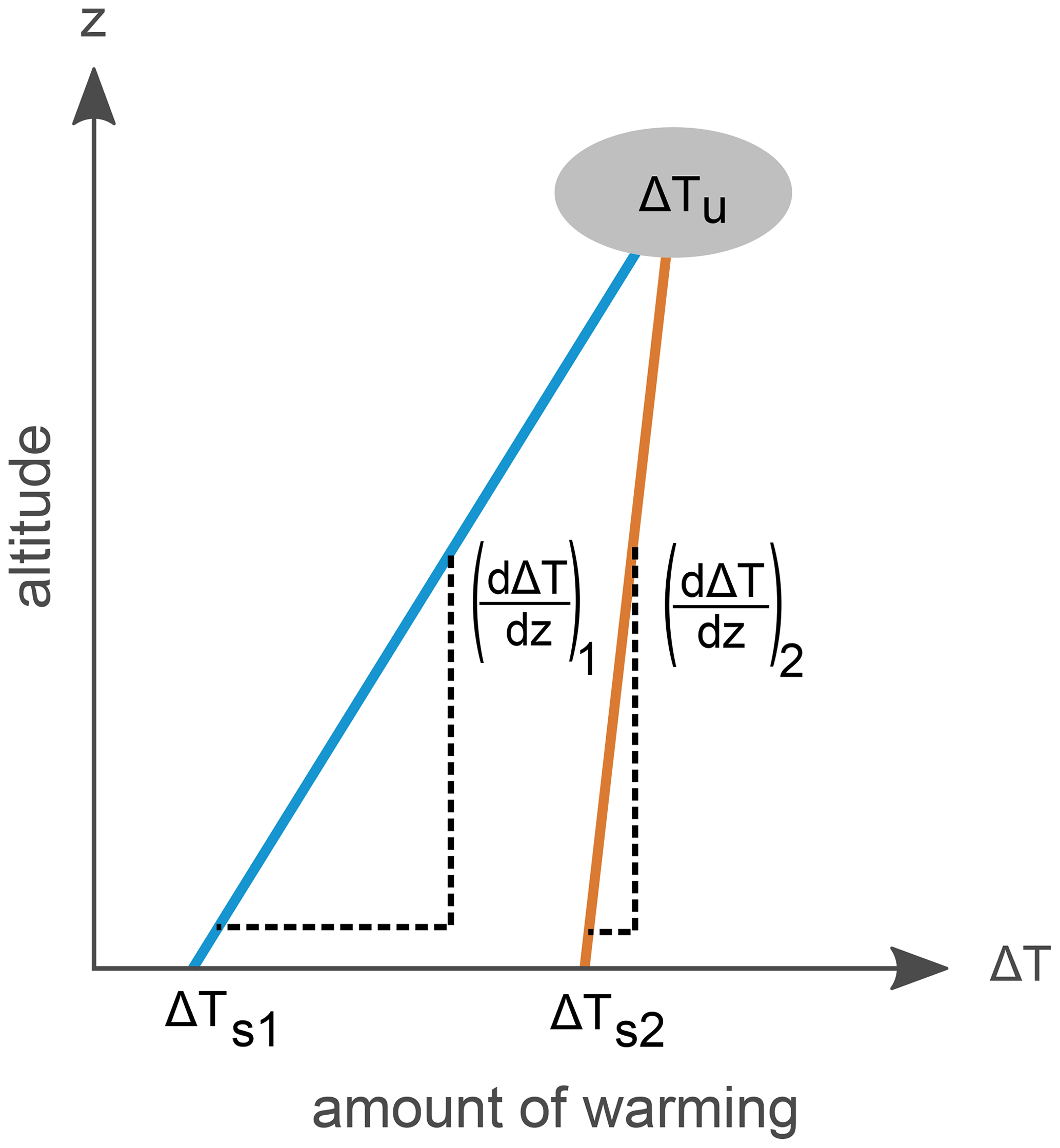
Figure 1Geometrical illustration of how lapse-rate changes are related to surface warming. The blue line shows a large lapse-rate change, as expected over the ocean, and the orange line a small lapse-rate change , as expected over land. We assume that the warming in the upper troposphere (ΔTu) is similar in both cases. From this assumption, it geometrically follows that the amount of surface warming is large (ΔTs2) where the lapse-rate change is small, and the surface warming is small (ΔTs1) where the lapse-rate change is large.
The influence of lapse-rate changes on the land–ocean warming contrast, displayed in Fig. 1, has been described mostly for tropical regions for two main reasons. First, the current tropical atmospheric stratification is governed by the moist-adiabatic lapse rate in all seasons (Xu and Emanuel, 1989; Schneider, 2007; Williams et al., 2009). Consequently, future changes in the moist-adiabatic lapse rates will be crucial. In summer, however, also the stratification in mid-latitudes seems to be governed by the moist-adiabatic lapse rate (Korty and Schneider, 2007; Frierson and Davis, 2011; Zamora et al., 2016). The second reason is that tropical upper tropospheric horizontal temperature gradients are small as a result of the small Coriolis parameter (Charney, 1963, 1969; Sobel and Bretherton, 2000). Therefore, we expect greenhouse-gas-driven upper tropospheric temperature changes to be horizontally homogeneous. In contrast, the spatial pattern of upper tropospheric warming to be expected outside the tropics is less clear.
In regards to variations in surface warming over land, lapse-rate changes have recently been suggested to exert a major influence on the Mediterranean amplification (Kröner et al., 2017; Brogli et al., 2019a, b). The Mediterranean amplification describes enhanced warming in the summer season over land regions around the Mediterranean basin (Fig. 2a). Yet, we do not know if these findings are transferable to other land regions of the world that experience above-average surface warming.
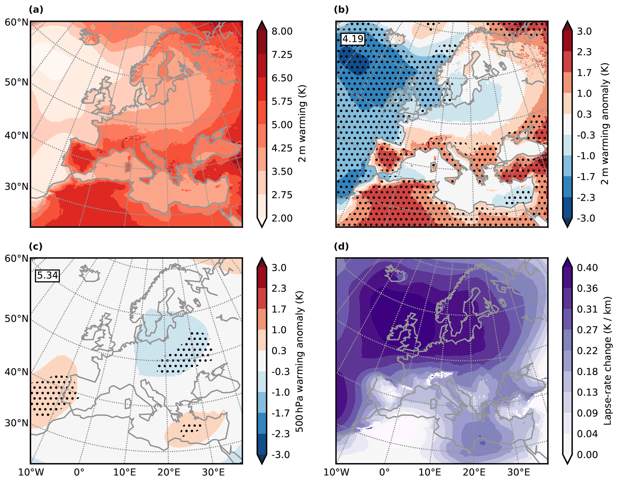
Figure 2European summer warming and associated lapse-rate changes in the 0.11∘ EURO-CORDEX ensemble for 1971–2000 vs. 2070–2099, assuming the RCP8.5 emission scenario. The summer season is taken as June, July, and August (JJA). (a) Mean summer 2 m warming of 15 EURO-CORDEX simulations shown as absolute values. (b) The same 2 m warming shown in (a) but expressed as warming anomaly or deviation from the domain mean. Red colors denote above-domain-mean warming and blue colors below-domain-mean warming. The number in the upper left of the map shows the domain-mean warming in kelvin. Stippling shows regions where all simulations agree on the sign of the warming anomaly. Overall, panel (b) highlights the pattern of the warming shown in panel (a). (c) Same as in panel (b) but on 500 hPa. (d) Lapse-rate changes expressed as warming difference between 500 and 850 hPa in kelvin per kilometer (K km−1) for the simulation ensemble shown in panels (a)–(c).
In this article, we build upon the previous results to demonstrate how lapse-rate changes govern the Mediterranean amplification. We present novel idealized simulations that demonstrate this causality more clearly than our previous simulations. Also, we show multi-model evidence for this causality. Additionally, we present evidence that lapse-rate changes are a driver for above-average land warming during the summer season in mid-latitudes and tropics across both the Northern Hemisphere and Southern Hemisphere. The findings originate from streamlined idealized simulations and the analysis of regional climate model (RCM) and global climate model (GCM) ensembles.
2.1 Analysis of CORDEX simulations over Europe
We analyze RCM simulations from the European Coordinated Regional Climate Downscaling Experiment (EURO-CORDEX) ensemble (Jacob et al., 2014, 2020). We use a total of 32 simulations performed with five different RCMs, driven by nine different GCM simulations from the Coupled Model Intercomparison Project Phase 5 (CMIP5) ensemble (Taylor et al., 2012). The EURO-CORDEX simulations feature horizontal resolutions of 0.44 or 0.11∘. Further details can be found in Table A1. All the downscaled GCM simulations assume the high-emission scenario RCP8.5 (Moss et al., 2010). We assess the 30-year seasonal average temperature changes between 2070–2099 and 1971–2000.
2.2 Idealized simulations over Europe
To establish the causality between lapse-rate changes and the European summer warming, we perform simulations using the regional climate model COSMO-CLM version 4.8 (CCLM4.8), which is the model of the Consortium for Small-Scale Modeling, COSMO (Baldauf et al., 2011), in climate mode (Rockel et al., 2008). The CCLM4.8 simulations feature a horizontal resolution of 0.44∘ (ca. 50 km), use 40 stretched vertical levels, and are covering the European domain following the EURO-CORDEX framework (Jacob et al., 2014, 2020). The simulations extend related experiments used in Kröner et al. (2017); Brogli et al. (2019a, b).
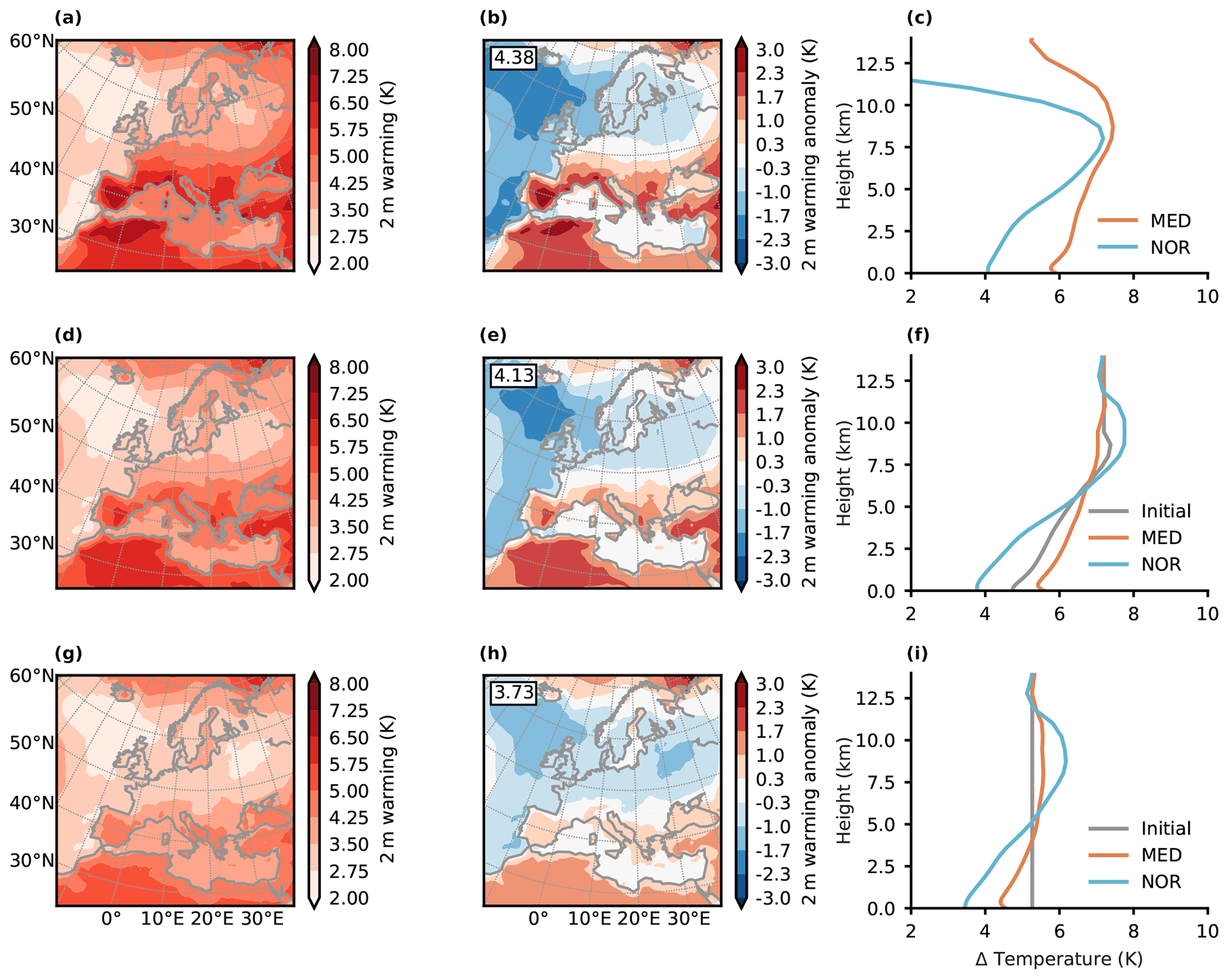
Figure 3Idealized simulations demonstrating the importance of tropospheric lapse-rate changes for European surface summer (JJA) warming anomalies. (a) Mean summer 2 m warming for full climate change (FCC), which is the mean of two RCM simulations dynamically downscaling two different GCMs assuming RCP8.5. We assess the warming between 2070–2099 and 1971–2000. (b) Same as panel (a) but showing 2 m warming anomaly (deviation from the domain mean given in the upper left of the map). (c) Mean vertical profiles of the summer temperature changes for the simulations shown in panels (a) and (b) for Mediterranean (orange line) land grid points (MED; between 30 and 44∘ N) and northern European (blue line) land grid points (NOR; between 55 and 70∘ N). (d–f) Same as in panels (a)–(c) but for TDLR, which is the mean of two idealized simulations, where the mean vertical warming profile as shown by the gray line in panel (f) is imposed on all lateral boundary grid points of the RCM simulations for 1971–2000. (g–i) Same as panels (d)–(f) but for TD that differs from TDLR by the imposed a vertically uniform warming profile shown by the gray line in panel (i).
2.2.1 Characteristics of idealized simulations
The following list contains the key characteristics of the simulations performed.
-
We perform regular transient regional climate simulations with CCLM4.8, where we downscale the two GCMs MPI-ESM-LR (Stevens et al., 2013) and HadGEM2-ES (The HadGEM2 Development Team, 2011) and analyze the mean of the two simulations. To assess climate change, we select two time slices which we call CTRL and SCEN. CTRL is the 1971–2000 period and SCEN the 2070–2099 period assuming RCP8.5. FCC = SCEN − CTRL is used to quantify temperature changes, where the abbreviation FCC stands for full climate change and will be used in the remainder of the article.
-
TD is the mean thermodynamic response of two idealized simulations where a vertically uniform warming profile is imposed at the lateral boundaries of CTRL. The shape of the vertical warming profile can be seen in Fig. 3i (gray line). The same profile is imposed on every lateral boundary grid point.
-
TDLR is the second set of idealized simulations where both the large-scale thermodynamic and lapse-rate change are imposed at the lateral boundaries of CTRL. The profile imposed on all boundary grid points is shown in Fig. 3f.
The idea behind the idealized experiments is the following: by comparing TD and TDLR we can quantify the influence of large-scale lapse-rate changes on the simulation result, as this is the only difference between the simulations. Simulated future changes that go beyond thermodynamic and lapse-rate changes, most prominently circulation and other dynamic changes, can be assessed by comparing TDLR and FCC. Figure A1 shows a comparison between circulation changes in TDLR and FCC and confirms that circulation changes are almost absent in TDLR.
2.2.2 Technical implementation of idealized simulations
The imposed warming profiles in TD and TDLR are derived from the domain-mean warming of FCC and include a representation of the annual cycle of the warming (Brogli et al., 2019a, b). In TDLR, the domain-mean warming of FCC on every tropospheric model level is imposed, and constant warming is imposed above the approximate average height of the tropopause. In TD, the mean warming of FCC, determined on the model level closest to 850 hPa, is imposed on all model levels. The annual cycle of SST changes is identically prescribed in TD and TDLR as a lower boundary condition and derived from the two-dimensional pattern of SST changes in FCC. For both atmospheric and ocean temperatures, the 30-year daily mean changes from FCC are converted to the prescribed annual cycle using a spectral filter as described in Bosshard et al. (2011). When changing the temperature in TD or TDLR experiments, we change the humidity assuming constant relative humidity. Also, the pressure is adjusted according to the hydrostatic balance (Schär et al., 1996). To quantify TD and TDLR, two different simulations, based on either the climate change signal of MPI-ESM-LR or HadGEM2-ES, have been performed and subsequently averaged for presentation. In the idealized experiments, the greenhouse gas concentrations have been adapted to match SCEN (Kröner et al., 2017).
2.3 Analysis of CMIP6 simulations
For global analysis, we include state-of-the-art GCM simulations from the Coupled Model Intercomparison Project Phase 6 (CMIP6) (Eyring et al., 2016), but we also provide a comparison against the CMIP5 (Taylor et al., 2012) ensemble (in Fig. A2). We use CMIP6 simulations assuming the emission scenario SSP5-8.5 (O'Neill et al., 2016), which is close to RCP8.5. For the analysis, all CMIP6 simulations have been regridded to a common 1.4∘ grid. In all simulations, the 30-year seasonal average temperature change between 2070–2099 and 1971–2000 is used to quantify climate change. A list of all CMIP6 simulations used is provided in Table A1.
Both the CMIP6 and EURO-CORDEX atmospheric data are available on pressure levels. Yet, to analyze lapse-rate changes (K m−1) the warming at the same geometrical height is more appropriate. For the quantification of lapse-rate changes we convert pressure levels to geometrical height.
3.1 European summer climate change in the EURO-CORDEX ensemble
The Mediterranean amplification is a striking and robust feature in projections of the European summer climate (Fig. 2a) from the EURO-CORDEX RCM ensemble. Following the high-emission scenario RCP8.5, some Mediterranean areas warm up to 3 K more than the domain average (Fig. 2b). In contrast to the Mediterranean, northern European land areas typically exhibit below-domain-mean summer warming (Fig. 2b). In the middle to upper troposphere, spatial variations in summer warming are negligible, as opposed to the surface (Fig. 2c). Regions characterized by small lapse-rate changes (Fig. 2d) in EURO-CORDEX coincide with regions of amplified surface warming (Fig. 2a and b). Figure 2 qualitatively indicates that different lapse-rate changes are connected to surface warming variations in Europe during summer.
3.2 Idealized simulations for Europe
The causal effect that lapse-rate changes have on the Mediterranean amplification is demonstrated in Fig. 3, showing the three pairs of simulations FCC, TDLR, and TD (see Sect. 2.2). The near-surface warming and warming anomaly of the regular downscaling simulations FCC (Fig. 3a and b) are in good agreement with EURO-CORDEX (Fig. 2a and b). From vertical profiles of the summer temperature change for FCC (Fig. 3c) we note that the warming is maximal at altitudes close to the tropopause. Also, in the upper troposphere, the warming is similar for northern Europe and the Mediterranean. Yet, the lapse-rate changes are different over the Mediterranean and northern Europe. In connection with a weak lapse-rate change, the surface warming in the Mediterranean is similar to the upper-tropospheric maximum and thus relatively high (Fig. 3c). Over northern Europe, the lapse-rate change is stronger and the surface warming smaller than over the Mediterranean. In general, the vertical warming profiles generated by the model (Fig. 3c) are very similar to the idealized picture shown in Fig. 1.
The Mediterranean amplification is well reproduced by TDLR (Fig. 3d–f), the idealized simulations that are forced with a large-scale tropospheric lapse-rate change. In contrast, the Mediterranean amplification is clearly weaker in TD where we prescribe no large-scale lapse-rate changes (Fig. 3g–i). Quantitatively, the warming contrast between the Mediterranean and northern Europe is around 1 K weaker in TD than TDLR. The absolute warming in the Mediterranean is ∼5.6 K in TDLR and ∼4.5 K in TD, while it is ∼5.9 K in FCC.
To understand the reason for the difference between the two idealized simulations, we compare the respective vertical warming profiles (Fig. 3f and i). By design, the shape of the initial warming profile imposed at the lateral boundaries (shown by the gray lines in Fig. 3f and i) differs between the two simulations. In TDLR, the lapse-rate change in the Mediterranean dynamically weakened compared to the imposed profile and the surface warming increased as a consequence (Fig. 3f, orange vs. gray line). In northern Europe, we see the opposite, meaning that the lapse-rate change simulated in the domain interior is stronger than what was prescribed, and the surface warming has decreased in response (Fig. 3f, blue vs. gray line). In other words, for the Mediterranean, some of the warming imposed at the lateral boundaries has been dynamically redistributed from the upper troposphere to the lower troposphere and vice versa for northern Europe.
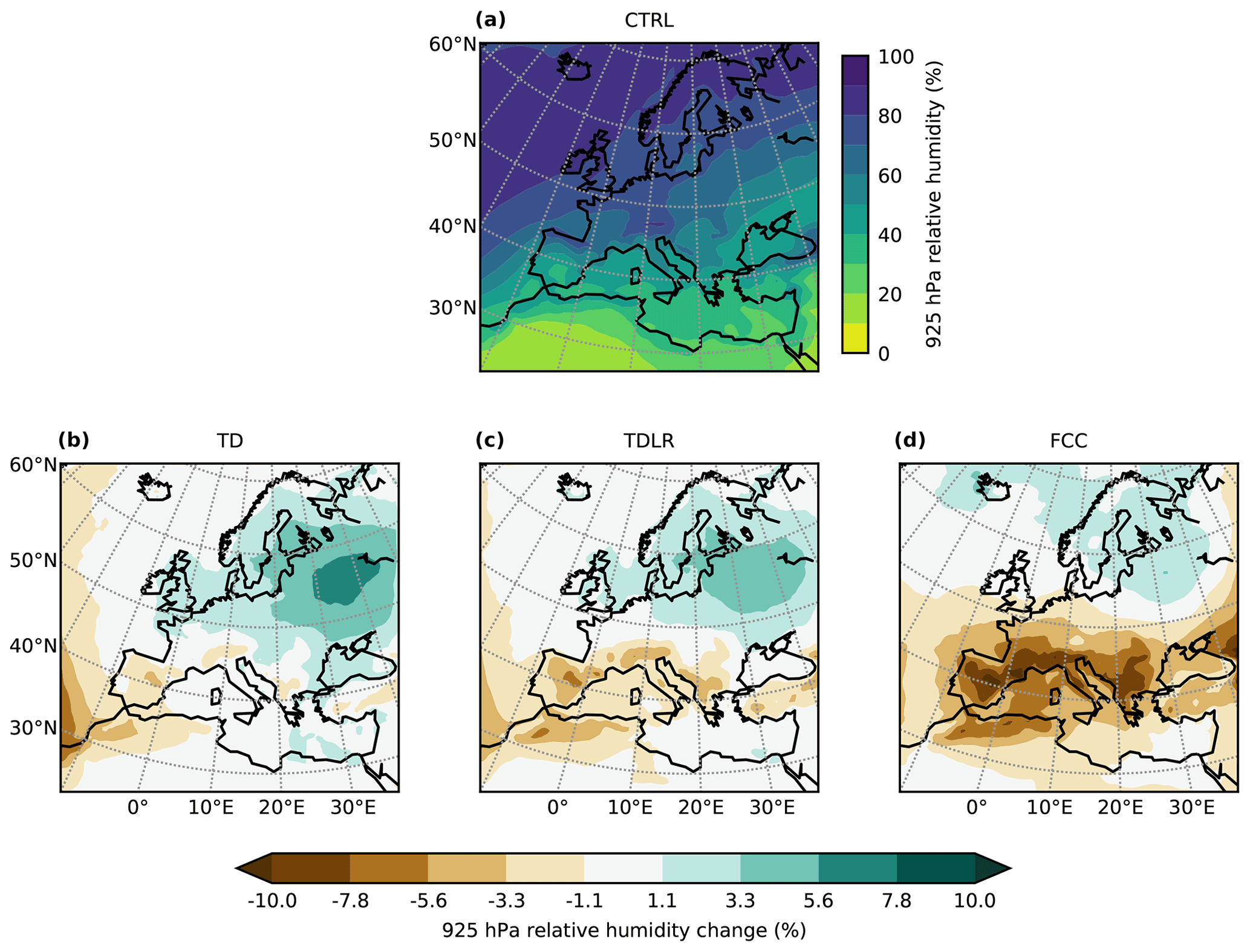
Figure 4Mean summer relative humidity in the historical CTRL simulation and changes in the idealized simulations. (a) Climatological relative humidity in CTRL for the average summer in the 1971–2000 period. (b) Change in relative humidity in the idealized TD simulation, representing RCP8.5 and the 2070–2099 period. (c) Same as panel (b) but for TDLR. (d) Same as panel (b) but for the FCC, which is the GCM-driven transient regional climate simulation.
In the TD experiments, where we impose vertically uniform warming at the lateral boundaries, the surface warming in both the Mediterranean and northern Europe is lower than what was imposed at the lateral boundaries (Fig. 3i) (Lenderink et al., 2019). This follows from similar dynamic alterations of the imposed warming profiles as in TDLR, meaning that also in TD the lapse rates adjust within the simulation domain compared to the warming profile imposed at the lateral boundaries. Also in TD, simulated lapse-rate changes are larger in northern Europe than the Mediterranean (Fig. 3i). This leads to a stronger surface warming in the Mediterranean in agreement with TDLR (Fig. 3g and h), but the absolute magnitude of the warming is over 1 K smaller in TD. An equally strong regional maximum in Mediterranean surface warming, as in TDLR or FCC, does not appear in the absence of a strong upper tropospheric warming maximum prescribed at the model boundary, even though we impose a comparatively high surface warming of ∼5.3 K (Fig. 3i) and the land–surface feedbacks in the model are fully interactive.
Summarizing Fig. 3, we find that two decisive changes in the climate system are needed to simulate the Mediterranean amplification. First, a strong and horizontally uniform large-scale upper tropospheric warming must be present. In our simulation this corresponds to the high warming (>7 K) at altitudes above 8 km, which is imposed in TDLR but not TD. Second, the lapse-rate changes are dynamically altered during the simulation depending on the European region and directly connected to the extent of summer surface warming.
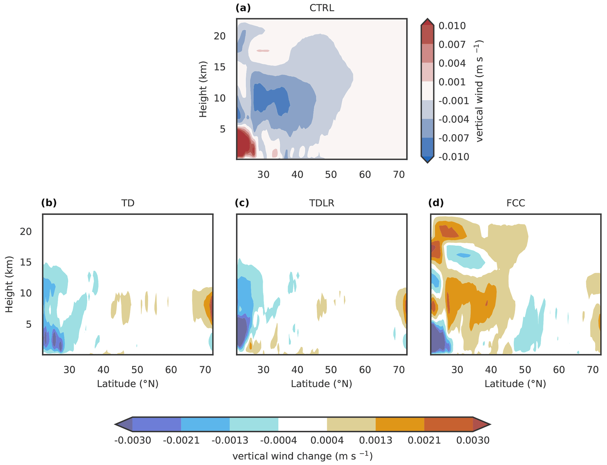
Figure 5Meridional cross section of mean summer vertical wind (positive values mean upward motion) in the historical CTRL simulation and changes in the idealized simulations. (a) Vertical wind in CTRL for the average summer in the 1971–2000 period. (b) Change in vertical wind in the idealized TD simulation, representing RCP8.5 and the 2070–2099 period. (c) Same as panel (b) but for TDLR. (d) Same as panel (b) but for the FCC, which is the GCM-driven transient regional climate simulation. This figure shows only data from the simulations based on the GCM HadGEM2-ES since the necessary three-dimensional model output was only stored for these simulations.
Since the Mediterranean is dryer in summer than northern Europe (Fig. 4), the dynamic alteration of the lapse-rate change profile supports the idea that moisture availability controls the strength of the lapse-rate changes in mid-latitudes during summer (Joshi et al., 2008; Fasullo, 2010; Byrne and O'Gorman, 2013a, b, 2018; Brogli et al., 2019a). The simulated local adjustment of lapse rates across the troposphere suggests that the European summer atmosphere is vertically mixed by local convection and subsidence. Lapse-rate changes are thus connected to the decrease in the moist-adiabatic lapse rate at warmer temperatures and radiative-convective equilibrium (Held and Soden, 2000). Small lapse-rate changes may occur where moist-adiabatic vertical mixing is inhibited by dry conditions and temperature-independent dry-adiabatic mixing plays a larger role. This is likely the case in the Mediterranean summer season, where the relative humidity is around 40 % (Fig. 4a). Moist-adiabatic vertical motions are infrequent (due to low moisture availability), and thus vertical warming gradients are small (there would be no vertical warming gradient if vertical mixing of warming throughout the troposphere was entirely dry adiabatic). In northern Europe, the summer season relative humidity is around 80 % (Fig. 4a) and is projected to increase further (Fig. 4b–d). Thus, vertical mixing in this region is more likely to follow a moist adiabat, which acts to change the lapse rates. The resulting substantial vertical warming gradients then lower the surface warming relative to the Mediterranean, according to the simulations shown in Fig. 3. Note that regional climatological differences in relative humidity as visible in Fig. 4a as well as relative humidity changes in response to warming (Fig. 4b–d) can contribute to the differences in lapse-rate changes projected by simulations. Yet, in both TD and TDLR we observe quite moderate changes in relative humidity compared to FCC (Fig. 4b and c vs. d). Therefore, it is likely that in our idealized simulations, the climatological spatial differences in moisture availability are crucial to induce changes in lapse rates. Despite the presented evidence, from our simulations alone, we are unable to diagnose that humidity differences are the ultimate cause of the different lapse-rate changes simulated within the model domain. Yet, this connection has been shown theoretically and in idealized simulations in earlier studies (Joshi et al., 2008; Byrne and O'Gorman, 2013a, 2018; Buzan and Huber, 2020).
Lapse-rate changes affect the vertical stratification and thereby vertical motions in the atmosphere, which is further explored in Fig. 5. From the previous findings in Fig. 3f and i we observed that the tropospheric warming imposed at the lateral boundaries is vertically redistributed within the simulation domain. A remaining question is if there are important dynamic adjustments in the idealized simulations that control the vertical exchange (e.g. increased subsidence). Figure 5 shows the vertical wind (w) in the historical CTRL simulation along with the changes in TD, TDLR, and FCC for the simulations based on HadGEM2-ES. In the historical climatological summer mean our simulations show subsidence in the southern part of the domain and no mean vertical wind in the northern part of the domain (Fig. 5a), which suggests that in the north upward and downward winds cancel on climatological timescales as is characteristic for the extratropics. Neither TD nor TDLR show substantial changes in vertical wind (Fig. 5b and c). In contrast, the subsidence slightly weakens in FCC (Fig. 5d). Thus, in TD and TDLR surface warming contrasts develop without substantial dynamic changes (Figs. 5 and A1). Physically we can interpret the extra warming in the southern part of the domain using the thermodynamic equation. When written using potential temperature θ, this is
where denotes the three-dimensional wind vector and the diabatic heating rate. Equation (1) is applied to the slowly evolving mean flow, and will thus include eddy contributions. Consider now the effect of the term . For the sake of the argument, we assume it is the dominating term, i.e. . In the simulations TD and TDLR w remains almost constant (Fig. 5b and c). However, the increased stratification implies that the contribution of to the local warming increases as well. In essence, the same subsidence within an enhanced stratification implies an increased warming. The argument illustrates that the extra warming in the southern part of the domain results essentially from adiabatic descent. Since we only change at the lateral boundaries in the TDLR simulation, this argument is especially relevant in TDLR.
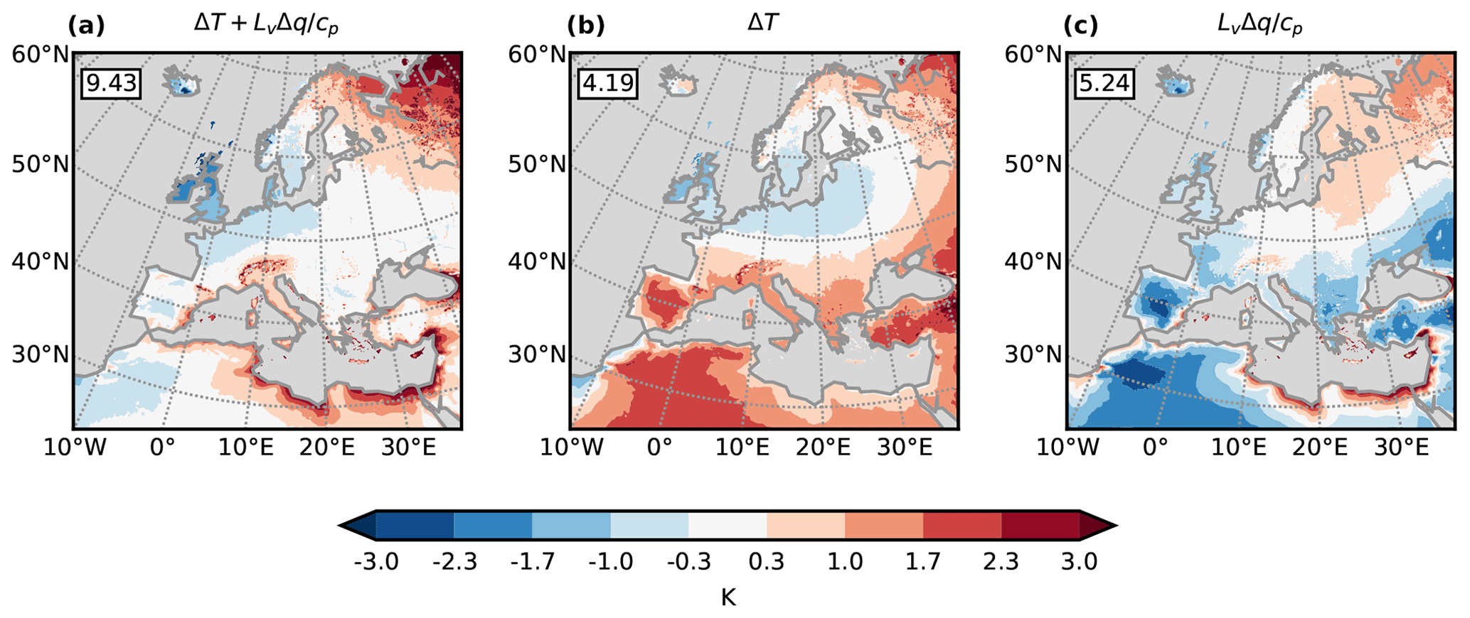
Figure 6Decomposition of the anomaly of surface moist enthalpy (H) changes in the 0.11∘ EURO-CORDEX ensemble for the summer season over land. (a) Overall anomaly (deviation from the domain mean) of the change in moist enthalpy, normalized by the specific heat of air (cp) to yield the unit kelvin. Thus, the surface moist enthalpy change has been computed as . The anomalies of the two components of H are shown separately. Panel (b) shows the anomaly of ΔT, while panel (c) shows the anomaly of . Gray shading shows ocean areas which are masked to improve the clarity.
Bringing together the results from Figs. 3–5, we interpret the results as follows: warming which we artificially impose in the idealized simulations is vertically redistributed throughout the troposphere. The vertical motions required to achieve the redistribution of the warming are already present during summer in the CTRL simulation (Fig. 5). The warming and moistening of the atmosphere in the TD simulation suffices to induce lapse-rate changes. These lapse-rate changes are more pronounced in present-day moist regions than in dry regions (Figs. 3i and 4a) because the vertical mixing follows the temperature-dependent moist-adiabatic lapse rate more frequently in moist regions. While in both TD and TDLR the lapse rates locally adjust according to the near-surface humidity and in both simulations lead to an amplification of the Mediterranean warming, the very high warming levels of more than 6 K are reached only in TDLR because here we prescribe a stronger homogeneous upper-tropospheric warming than in TD. This upper-tropospheric warming affects the surface warming trough adiabatic descent in the Mediterranean. We suggest that only the combination of the strong large-scale upper-level warming and vertically near-adiabatic redistribution of the warming evokes the Mediterranean amplification.
Overall, during European summer, the entire troposphere is relevant to understand the surface warming pattern: from TD, we can observe that surface moisture gradients influence the warming up to 10–12 km height (Fig. 3i). On the other hand, the extra upper tropospheric warming introduced in TDLR strongly affects near-surface warming levels (Fig. 3f).
As discussed, the homogeneous and strong upper tropospheric warming is a key process in understanding southern European summer warming. Yet, it may be surprising that the middle to upper tropospheric temperature change in summer over Europe is spatially almost uniform. While this seems clear in the simulations we analyzed, the physical reasons behind it remain more speculative and can be an avenue for future research. Generally, a strong upper tropospheric summer warming can be expected, since most of the globe is covered by oceans where one would expect strong lapse-rate changes due to the abundance of moisture. The uniformity of the warming could be related to the weak Equator-to-pole temperature gradient in summer, which also results in weak baroclinicity, implying that warming gradients will also be small. Also, the long 30-year periods that we averaged to obtain the results might act to smooth upper atmospheric warming gradients generally.
3.3 Changes in moist enthalpy in EURO-CORDEX
Previously, we argued that the differential importance of moist- and dry-adiabatic vertical mixing controls the magnitude of summer lapse-rate changes and regulates the surface warming. A similar argument can be made when analyzing the change in moist enthalpy (Berg et al., 2016; Byrne and O'Gorman, 2018; Matthews, 2018). The moist enthalpy is given by , where cp is the specific heat of air, T is temperature, Lv is the latent heat of vaporization, and q is the specific humidity. In a warming climate, the change in moist enthalpy quantifies the combined effect of changes in internal energy given by temperature changes (cpΔT) and the change in latent energy, which could be released by condensation if air was lifted to the top of the atmosphere (LvΔq).
Figure 6 shows the spatial anomalies of the overall change in moist enthalpy (ΔH) and the two components cpΔT and LvΔq separately. The data are from the EURO-CORDEX ensemble and the summer season (JJA). Note that over land, the simulations project a spatially relatively homogeneous change in H (Fig. 6a). This means that total amount energy used for raising temperatures or humidity is similar throughout the European continent. Yet, the change in internal energy or temperature shows a regional maximum in the Mediterranean (Fig. 6b), while the change in latent energy is smaller in the Mediterranean than elsewhere in the domain (Fig. 6c). The change in latent energy describes the potential for latent energy release by convection, which is also the root of lapse-rate changes. Thus, the change in moist enthalpy supports the notion that the additional available energy connected to climate change in the Mediterranean rather translates to an increase in surface temperature (cpΔT) than to an increase in convective latent heat release (LvΔq) and vice versa for northern Europe. The below-average increase in Δq (Fig. 6c) is a clear sign for limited moisture availability in the Mediterranean, because from the climatological temperatures alone, one would expect an above-average increase in Δq in the relatively warm Mediterranean (the warmer air could potentially carry more water vapor). This below-average increase in q also implies a decrease in near-surface relative humidity, which means that the limited present-day Mediterranean water availability (Cramer et al., 2018) will intensify. Thus, both the present-day dryness (Fig. 4) and a low increase in atmospheric moisture limit the increase in latent energy in the Mediterranean.
3.4 Statistical analysis of EURO-CORDEX simulations
The results shown in Figs. 2–6 suggest that lapse-rate changes are crucial for determining European summer surface warming anomalies in the multi-model mean in EURO-CORDEX and our RCM simulations. By statistically analyzing lapse-rate changes in 32 single members of the EURO-CORDEX ensemble, we here confirm the robustness of these findings and the transferability to different RCMs. We consider the full ensemble (Table A1) and a subset of 14 simulations performed with the RCM RCA4 (Kjellström et al., 2016) that use identical parameterization schemes and only differ in the large-scale forcing from different GCMs (Table A1).
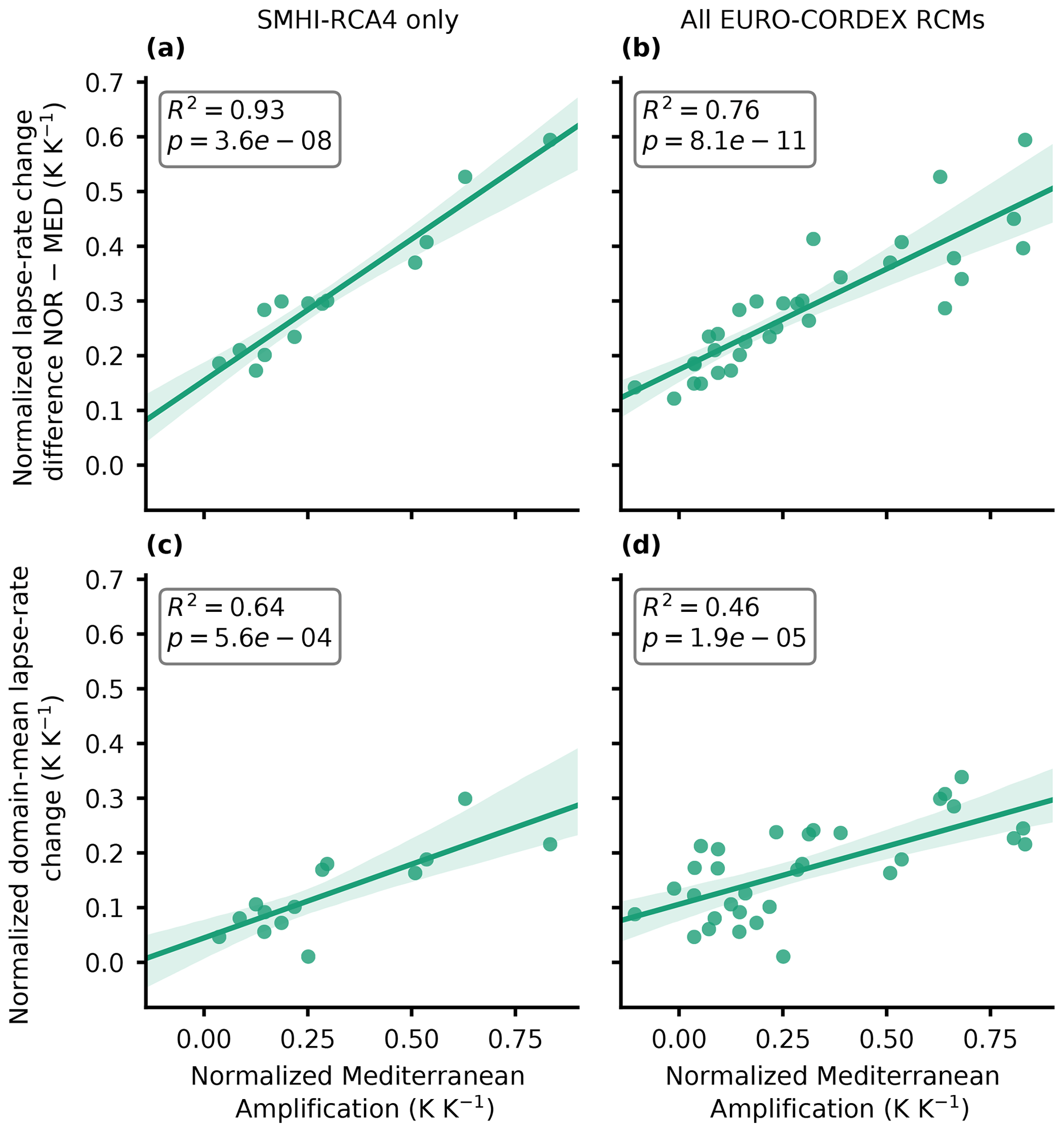
Figure 7Linear regression linking the enhanced Mediterranean summer 2 m warming to lapse-rate changes in the EURO-CORDEX ensemble. (a, b) Regression linking the Mediterranean amplification and differences in lapse-rate changes between northern Europe (NOR) and the Mediterranean (MED) over land. (c, d) Regression linking the Mediterranean amplification to the European-scale domain-mean lapse-rate change. (a, c) A subset of the EURO-CORDEX ensemble using one single regional climate model, namely SMHI-RCA4. (b, d) All EURO-CORDEX simulations that were used in this study (Table A1). Each dot represents a simulation with a horizontal resolution of 0.11 or 0.44∘. The figure is based on summer-mean (JJA) changes between 1971–2000 and 2070–2099, assuming RCP8.5. We normalized both the Mediterranean amplification and lapse-rate changes with the domain-mean warming, yielding dimensionless values (KK). The lapse-rate changes have been computed as the difference between the 500 hPa warming and the 850 hPa warming. We evaluate the Mediterranean between 30 and 44∘ N and northern Europe between 55 and 70∘ N. The boxes in the upper left corner of the panels show the statistics of the linear regression fit, while the shadings show the 95 % confidence interval of the linear regression estimated by 1000-fold bootstrapping.
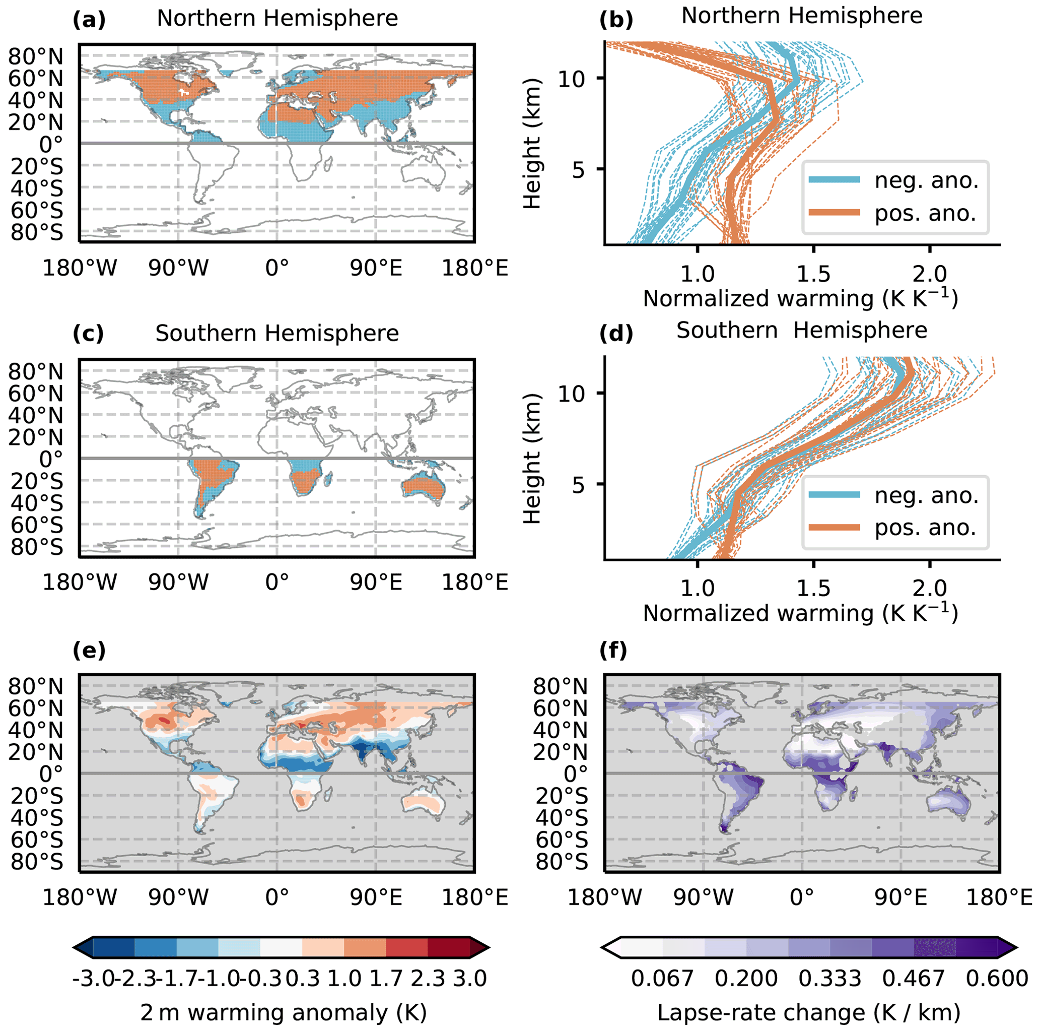
Figure 8Summer lapse-rate changes as projected by CMIP6 simulations. The changes are evaluated between 1971–2000 and 2070–2099, assuming the SSP5-8.5 scenario for JJA north of the Equator and December, January, and February (DJF) south of the Equator. (a) Map showing areas where the ensemble mean Northern Hemispheric summer near-surface warming is above (orange) and below (blue) average over land in the mid-latitudes and tropics (0–66∘ N). (b) Mean vertical profiles of summer warming in regions where the surface warming is above and below average (orange and blue profiles, respectively). The thin dashed lines show individual ensemble members, and the bold line shows the ensemble mean. The vertical warming profiles are normalized by every simulation's mean summer warming over land grid points on 925 hPa. (c) Same as panel (a) for the Southern Hemisphere (0–66∘ S). (d) Same as panel (b) for the areas shown in panel (c). (e) Map of mean land 2 m warming anomalies in the Northern Hemisphere and Southern Hemisphere during the respective summer season. Areas masked in the analysis are shown in gray. Red colors show above-average warming and blue below-average warming. (f) Map of lapse-rate changes evaluated as warming difference between 500 and 850 hPa (K km−1). Masked areas (sometimes due to high topography) are shown in gray.
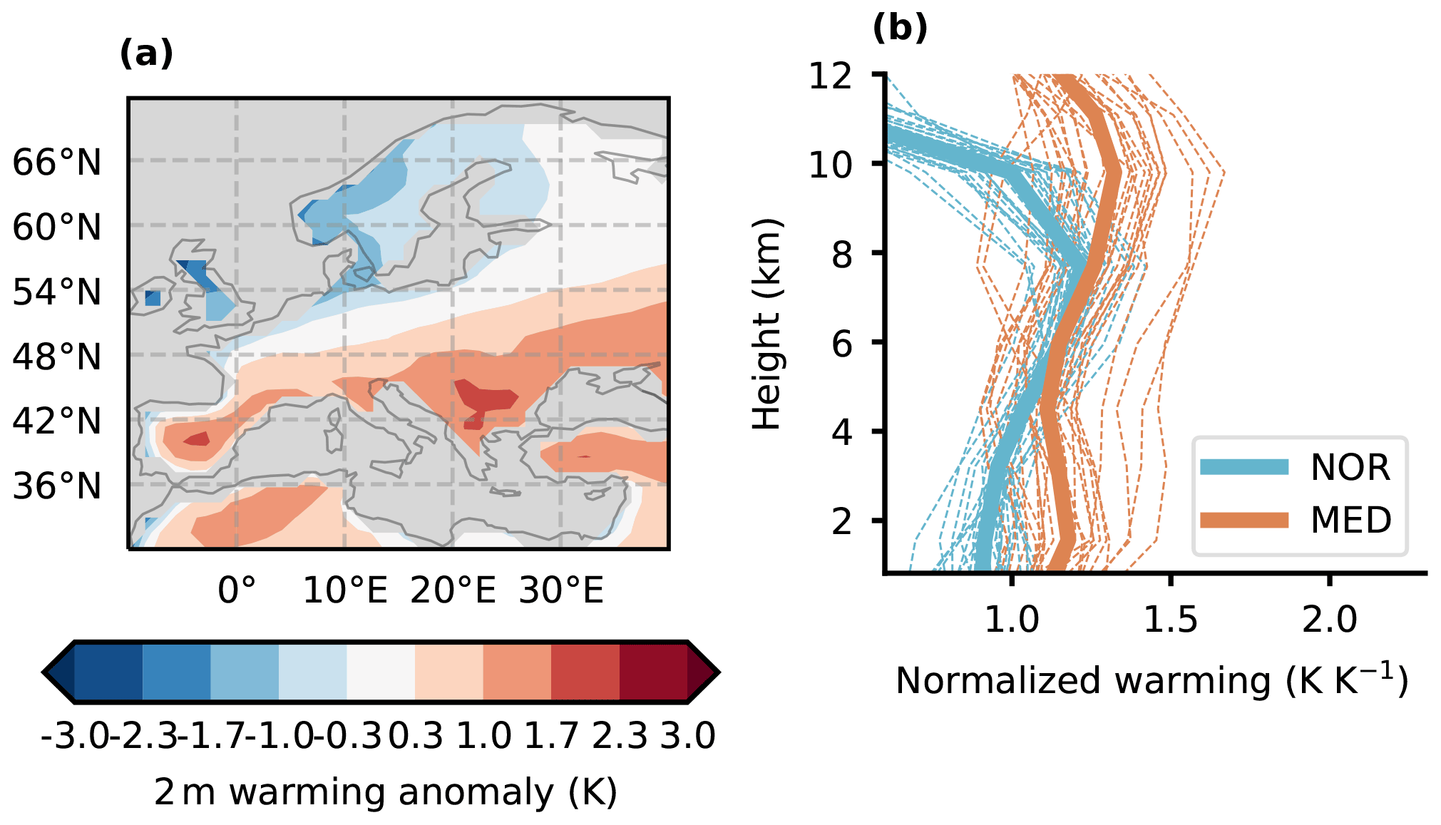
Figure 9The Mediterranean amplification in CMIP6 simulations. (a) Ensemble mean summer near-surface warming anomaly with respect to the ensemble mean of Northern Hemispheric land grid points (0–70∘ N). (b) Mean vertical warming profiles over the Mediterranean (MED; orange) and northern Europe (NOR; blue) in summer. The thin dashed lines show individual ensemble members, and the bold line shows the ensemble mean. The MED is evaluated between 30 and 44∘ N and 10∘ W and 40∘ E, while NOR is evaluated between 55 and 70∘ N and 0 and 40∘ E, and only land grid points are used. The warming has been normalized by the mean warming on 925 hPa over NOR and MED.
We show linear regressions in Fig. 7. Previously, we identified two core triggers for the Mediterranean amplification. First, the local lapse-rate changes over northern Europe must be larger than over the Mediterranean. Second, a strong homogeneous upper tropospheric warming must be present. The linear regressions support this idea (Fig. 7), showing that, first, the larger the difference in lapse-rate changes between northern Europe and the Mediterranean, the larger the Mediterranean amplification (Fig. 7a and b). Second, the larger the domain-mean lapse-rate change (i.e. more upper tropospheric warming compared to the surface), the larger the Mediterranean amplification (Fig. 7c and d). All the positive correlations found in Fig. 7 are statistically significant (p<0.0006) and feature R2 values ranging from 0.46 to 0.93. Thus, Fig. 7 supports the notion that in a variety of climate projections, mean lapse-rate changes and spatial differences in lapse-rate changes contribute to the magnitude of summer surface warming.
However, a remaining open question from Fig. 7 is what intrinsic differences between the simulations cause the different lapse-rate changes in the EURO-CORDEX ensemble members, especially in the ensemble using the same RCM. A limited body of research suggests that such intermodel differences might be related to regional SST warming differences in GCMs (Po-Chedley et al., 2018; Tuel, 2019). Different lapse-rate changes between models have also been suggested to be connected to differences in climate sensitivity (Ceppi and Gregory, 2017), which makes this question even more relevant.
The fact that lapse-rate changes are relevant in the context of European summer climate change raises the question of whether they are equally influential in other regions of the planet. To this end, we further explore surface warming anomalies and the connected lapse-rate changes in global climate simulations.
3.5 Analysis on global scale
Figure 8 shows end-of-century summer lapse-rate changes for all land regions of the world within the mid-latitudes and tropics (−66∘ S < latitude < 66∘ N) from the CMIP6 global simulation ensemble. Additionally, we verified the ability of CMIP6 models to reproduce the lapse-rate changes over northern Europe and the Mediterranean simulated by RCMs (Fig. 9). Generally, the CMIP6 models considered also exhibit the Mediterranean amplification (Figs. 9 and 8e) and show pronounced regional differences in lapse-rate changes.
The global analysis confirms that weak lapse-rate changes are connected to enhanced land–surface warming across the Northern Hemisphere and Southern Hemisphere in the summer season. During the Northern Hemispheric summer, the warming on an altitude of ∼8 km is similar in all regions (Fig. 8b). Regions characterized by above-average summer warming (Fig. 8a) robustly show comparably small lapse-rate changes (Fig. 8b). Lapse-rate changes in areas with below-average warming (Fig. 8a) are large (Fig. 8b). Above-average summer warming in the Northern Hemisphere is projected in central North America, the Mediterranean, northern Africa, the Middle East, and large parts of Central Asia (Fig. 8a and e). In contrast, CMIP6 models show below-average summer land warming and large lapse-rate changes in the tropics, northern Europe, and in high-latitude North America (Fig. 8a, e, and f), consistent with the analyses over Europe.
In the Southern Hemisphere, the summer lapse-rate changes, and the resulting surface warming anomalies are in line with previous findings (Fig. 8c and d). Lapse-rate changes are stronger in regions exhibiting below-average warming in comparison to regions with above-average warming, which is robust in all simulations considered (Fig. 8d). Thus, lapse-rate changes are closely related to the pattern of summer temperature change, also in the Southern Hemisphere. One remarkable difference is that the average altitude at which the warming starts to be spatially homogeneous occurs at ∼4 km in the Southern Hemisphere, which is lower than in the Northern Hemisphere, where it is located at ∼8 km (Fig. 8b and d). Also, surface warming anomalies are less pronounced (Fig. 8e). We assume that this is because the fraction of oceans is much larger in the Southern Hemisphere, which reduces the altitude up to which land surface inhomogeneities can influence temperature changes. In the Southern Hemisphere, the regions connected to above-average land warming are continental areas in South America, South Africa, and Australia. Below-average warming is found along the coast of the previously mentioned regions and New Zealand (Fig. 8c and e). Disparities in lapse-rate changes between continental and coastal areas (Fig. 8f) are a further indication that the moisture availability influences the strength of lapse-rate changes as regions along the coast tend to be more humid than continental regions.
The findings presented for the CMIP6 ensemble in Fig. 8 are in agreement with the results obtained using the CMIP5 ensemble (Fig. A2), although the magnitude of surface warming anomalies has increased from CMIP5 (RCP8.5) to CMIP6 (SSP5-8.5). In summary, the qualitative analysis shown in Fig. 8 suggests that the findings for the European region (Figs. 2–7) are likely transferable to other regions on the globe, and future more specific regional research is desirable.
We find that variations in the vertical warming with climate change, given by atmospheric lapse-rate changes, are decisive for the understanding of enhanced or reduced regional greenhouse-gas-driven surface warming during summer. We provide additional evidence for this finding in Europe, where we demonstrate that both a strong large-scale upper tropospheric warming and regionally modified lapse-rate changes are key reasons for the Mediterranean amplification. The results are consistent across CORDEX and CMIP climate model ensembles. Additionally, we showed that lapse-rate changes are closely connected to summer surface warming anomalies on a global scale over land areas. The connection between lapse-rate changes, which are governed by the well-understood temperature dependence of the moist-adiabatic lapse rate, and summer warming anomalies increases our confidence that climate models can accurately project such anomalies.
Our results suggest that lapse-rate changes have more extensive consequences than previously thought. First, lapse-rate changes significantly contribute to the summer-season surface warming pattern in mid-latitudes and the tropics. Second, lapse-rate changes influence surface warming patterns within land regions in addition to the land–ocean warming contrast. Tropospheric temperature and lapse-rate changes should thus be considered when assessing the causes for surface warming anomalies, in addition to surface processes. Since evidence from multiple studies points to a connection between surface moisture and lapse-rate changes (Joshi et al., 2008; Byrne and O'Gorman, 2013a, b, 2018; Brogli et al., 2019a, this study), it might be possible to use surface moisture as an observational constraint for future summer warming. Our study is solely based on climate change simulations. Therefore, an open task is to diagnose historical differences in lapse-rate changes from observations. It is, however, hard to estimate what level of warming is necessary for lapse-rate changes to be detected in observations, as this requires multiple long records of homogeneous upper-tropospheric measurements, which are sparse and prone to biases (Santer et al., 2005; Stickler et al., 2010; Thorne et al., 2011; Flannaghan et al., 2014; Santer et al., 2017).
Table A1Simulations used for analysis. The original simulations are regional climate modeling (RCM) experiments as described in Sect. 2.2, and the additional RCM simulations are from the EURO-CORDEX ensemble. Furthermore, global climate (GCM) simulations from the CMIP6 ensemble are used. Columns show the model name, the global driving simulation for RCMs, the realization for GCMs, and the horizontal resolution of the atmospheric model.
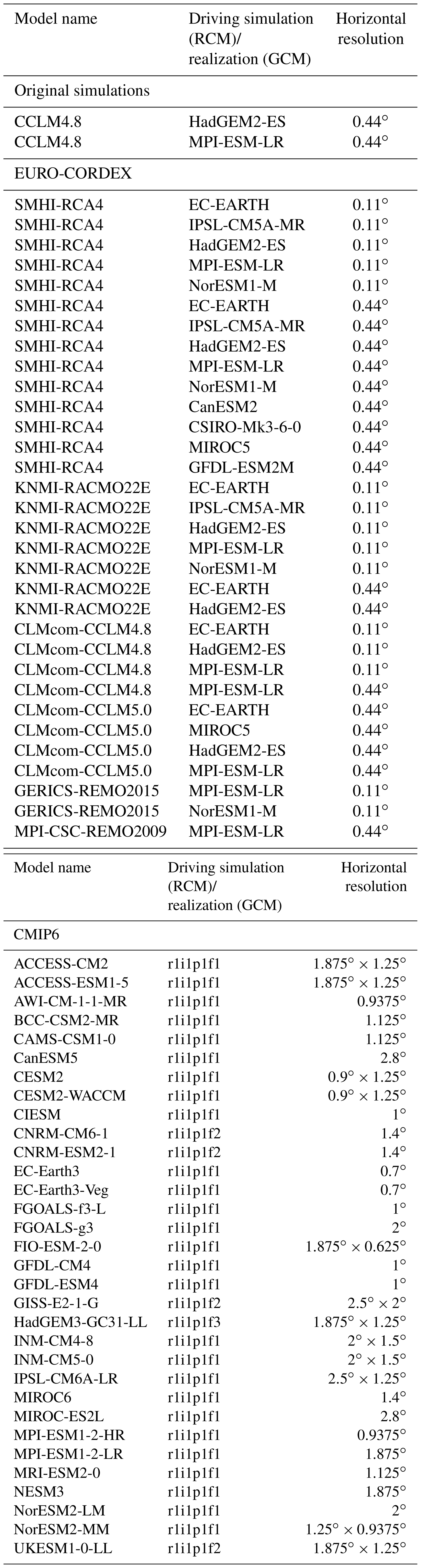
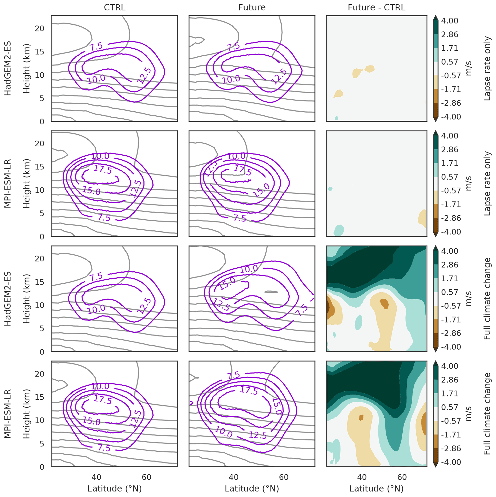
Figure A1Changes in the mean summer zonal winds in idealized simulations forced by thermodynamics and lapse-rate changes (named TDLR) compared to fully transient climate simulations (named FCC). The first and third row show CCLM4.8 simulations over Europe with climate changes derived from HadGEM2-ES. The second and fourth row show CCLM4.8 simulations based on MPI-ESM-LR. The upper two rows show simulations that have been forced with domain-mean lapse-rate changes and SSTs only (TDLR). The lower two rows show the corresponding transient climate simulations (FCC). (Left column) Meridional cross section of isotherms (gray contours every 10 K) and zonal wind (purple contours in m s−1) in the historical simulation (1971–2000). (Middle column) Same as the left column but for the future climate state (2070–2099). (Right column) Difference in zonal wind between the historical and future simulation.
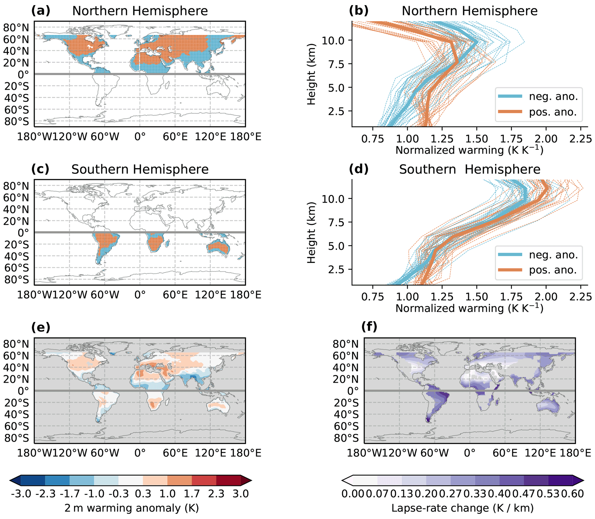
Figure A2Same as Fig. 8 but for an ensemble of CMIP5 simulations consisting of the following models: ACCESS1-0, ACCESS1-3, BCC-CSM1-1, BCC-CSM1-1-m, BNU-ESM, CanESM2, CESM1-BGC, CESM1-CAM5, CESM1-CAM5-1-FV2, CESM1-WACCM, CMCC-CESM, CMCC-CM, CMCC-CMS, CNRM-CM5, CSIRO-Mk3-6-0, FGOALS-g2, FIO-ESM, GFDL-CM3, GFDL-ESM2G, GFDL-ESM2M, GISS-E2-H, GISS-E2-H-CC, GISS-E2-R, GISS-E2-R-CC, HadGEM2-AO, HadGEM2-CC, HadGEM2-ES, INM-CM4, IPSL-CM5A-LR, IPSL-CM5A-MR, IPSL-CM5B-LR, MIROC5, MIROC-ESM, MIROC-ESM-CHEM, MPI-ESM-LR, MPI-ESM-MR, MRI-CGCM3, and MRI-ESM1.
The codes that are the basis for our idealized experiments are open source and can be obtained from https://doi.org/10.5281/zenodo.4890235 (Brogli and Vergara-Temprado, 2021). The weather and climate model CCLM is available free of charge for research applications (for more details see http://www.cosmo-model.org, Rockel et al., 2008). EURO-CORDEX, CMIP6, and CMIP5 data are available from ESGF nodes (https://esgf-data.dkrz.de/projects/esgf-dkrz; see Jacob et al., 2020; Eyring et al., 2016; Taylor et al., 2012).
RB, SLS, NK, and CS designed research. RB performed simulations. RB and NK analyzed data. RB, SLS, and CS wrote the article.
The contact author has declared that neither they nor their co-authors have any competing interests.
Publisher's note: Copernicus Publications remains neutral with regard to jurisdictional claims in published maps and institutional affiliations.
Many thanks to two anonymous reviewers who helped us with their constructive feedback to improve the article. We acknowledge PRACE for awarding us access to Piz Daint at the Swiss National Supercomputing Center (CSCS, Switzerland). Furthermore, we acknowledge the COSMO, CLM, and C2SM communities for developing and maintaining the RCM. We also acknowledge the World Climate Research Programme's working groups on regional climate and on coupled modeling, responsible for CORDEX and CMIP, and we thank the climate modeling groups for producing and making available their model output. We thank Urs Beyerle for preparing the CORDEX and CMIP data for our analysis and Paul O'Gorman for discussions on the topic of the article.
This research has been supported by the Horizon 2020 research and innovation program (CONSTRAIN, grant no. 820829) and the Schweizerischer Nationalfonds zur Förderung der Wissenschaftlichen Forschung (trCLIM, grant no. 192133).
This paper was edited by David Battisti and reviewed by two anonymous referees.
Baldauf, M., Seifert, A., Förstner, J., Majewski, D., Raschendorfer, M., and Reinhardt, T.: Operational Convective-Scale Numerical Weather Prediction with the COSMO Model: Description and Sensitivities, Mon. Weather Rev., 139, 3887–3905, https://doi.org/10.1175/MWR-D-10-05013.1, 2011. a
Barcikowska, M. J., Kapnick, S. B., Krishnamurty, L., Russo, S., Cherchi, A., and Folland, C. K.: Changes in the future summer Mediterranean climate: contribution of teleconnections and local factors, Earth Syst. Dynam., 11, 161–181, https://doi.org/10.5194/esd-11-161-2020, 2020. a
Berg, A., Findell, K., Lintner, B., Giannini, A., Seneviratne, S. I., Van Den Hurk, B., Lorenz, R., Pitman, A., Hagemann, S., Meier, A., Cheruy, F., Ducharne, A., Malyshev, S., and Milly, P. C.: Land-atmosphere feedbacks amplify aridity increase over land under global warming, Nat. Clim. Change, 6, 869–874, https://doi.org/10.1038/nclimate3029, 2016. a, b
Bosshard, T., Kotlarski, S., Ewen, T., and Schär, C.: Spectral representation of the annual cycle in the climate change signal, Hydrol. Earth Syst. Sci., 15, 2777–2788, https://doi.org/10.5194/hess-15-2777-2011, 2011. a
Brogli, R. and Vergara-Temprado, J.: broglir/pgw-python: First release (v1.0), Zenodo [code], https://doi.org/10.5281/zenodo.4890235, 2021. a
Brogli, R., Kröner, N., Sørland, S. L., Lüthi, D., and Schär, C.: The Role of Hadley Circulation and Lapse-Rate Changes for the Future European Summer Climate, J. Climate, 32, 385–404, https://doi.org/10.1175/JCLI-D-18-0431.1, 2019a. a, b, c, d, e
Brogli, R., Sørland, S. L., Kröner, N., and Schär, C.: Causes of future Mediterranean precipitation decline depend on the season, Environ. Res. Lett., 14, 114017, https://doi.org/10.1088/1748-9326/ab4438, 2019b. a, b, c
Buzan, J. R. and Huber, M.: Moist Heat Stress on a Hotter Earth, Annu. Rev. Earth Pl. Sc., 48, 623–655, https://doi.org/10.1146/annurev-earth-053018-060100, 2020. a, b
Byrne, M. P. and O'Gorman, P. A.: Land-ocean warming contrast over a wide range of climates: Convective quasi-equilibrium theory and idealized simulations, J. Climate, 26, 4000–4016, https://doi.org/10.1175/JCLI-D-12-00262.1, 2013a. a, b, c, d, e, f
Byrne, M. P. and O'Gorman, P. A.: Link between land-ocean warming contrast and surface relative humidities in simulations with coupled climate models, Geophys. Res. Lett., 40, 5223–5227, https://doi.org/10.1002/grl.50971, 2013b. a, b
Byrne, M. P. and O'Gorman, P. A.: Trends in continental temperature and humidity directly linked to ocean warming, P. Natl. Acad. Sci. USA, 115, 4863–4868, https://doi.org/10.1073/pnas.1722312115, 2018. a, b, c, d, e, f, g
Ceppi, P. and Gregory, J. M.: Relationship of tropospheric stability to climate sensitivity and Earth's observed radiation budget, P. Natl. Acad. Sci. USA, 114, 201714308, https://doi.org/10.1073/pnas.1714308114, 2017. a
Chadwick, R., Ackerley, D., Ogura, T., and Dommenget, D.: Separating the Influences of Land Warming, the Direct CO2 Effect, the Plant Physiological Effect, and SST Warming on Regional Precipitation Changes, J. Geophys. Res.-Atmos., 124, 624–640, https://doi.org/10.1029/2018JD029423, 2019. a
Charney, J. G.: A Note on Large-Scale Motions in the Tropics, J. Atmos. Sci., 20, 607–609, https://doi.org/10.1175/1520-0469(1963)020<0607:ANOLSM>2.0.CO;2, 1963. a
Charney, J. G.: A Further Note on Large-Scale Motions in the Tropics, J. Atmos. Sci., 26, 182–185, https://doi.org/10.1175/1520-0469(1969)026<0182:AFNOLS>2.0.CO;2, 1969. a
Collins, M., Knutti, R., Arblaster, J., Dufresne, J.-L., Fichefet, T., Friedlingstein, P., Gao, X., Gutowski, W., Johns, T., Krinner, G., Shongwe, M., Tebaldi, C., Weaver, A., and Wehner, M.: Long-term climate change: Projections, commitments and irreversibility, in: Climate Change 2013 the Physical Science Basis: Working Group I Contribution to the Fifth Assessment Report of the Intergovernmental Panel on Climate Change, edited by: Stocker, T., Qin, D., Plattner, G.-K., Tignor, M., Allen, S., Boschung, J., Nauels, A., Xia, Y., Bex, V., and Midgley, P., Cambridge University Press, Cambridge, United Kingdom and New York, NY, USA, 1029–1136, https://doi.org/10.1017/CBO9781107415324.024, 2013. a
Cramer, W., Guiot, J., Fader, M., Garrabou, J., Gattuso, J.-P., Iglesias, A., Lange, M. A., Lionello, P., Llasat, M. C., Paz, S., Peñuelas, J., Snoussi, M., Toreti, A., Tsimplis, M. N., and Xoplaki, E.: Climate change and interconnected risks to sustainable development in the Mediterranean, Nat. Clim. Change, 7, 972–980, https://doi.org/10.1038/s41558-018-0299-2, 2018. a
Diffenbaugh, N. S. and Giorgi, F.: Climate change hotspots in the CMIP5 global climate model ensemble, Climatic Change, 114, 813–822, https://doi.org/10.1007/s10584-012-0570-x, 2012. a
Eyring, V., Bony, S., Meehl, G. A., Senior, C. A., Stevens, B., Stouffer, R. J., and Taylor, K. E.: Overview of the Coupled Model Intercomparison Project Phase 6 (CMIP6) experimental design and organization, Geosci. Model Dev., 9, 1937–1958, https://doi.org/10.5194/gmd-9-1937-2016, 2016. a, b
Fasullo, J. T.: Robust land-ocean contrasts in energy and water cycle feedbacks, J. Climate, 23, 4677–4693, https://doi.org/10.1175/2010JCLI3451.1, 2010. a, b, c
Flannaghan, T. J., Fueglistaler, S., Held, I. M., Po-Chedley, S., Wyman, B., and Zhao, M.: Tropical Temperature Trends in AMIP Simulations and the Impact of SST Uncertainties, J. Geophys. Res.-Atmos., 119, 13327–13337, https://doi.org/10.1002/2014JD022365, 2014. a
Frierson, D. M. and Davis, N. A.: The seasonal cycle of midlatitude static stability over land and ocean in global reanalyses, Geophys. Res. Lett., 38, 1–6, https://doi.org/10.1029/2011GL047747, 2011. a
Good, P., Lowe, J. A., Andrews, T., Wiltshire, A., Chadwick, R., Ridley, J. K., Menary, M. B., Bouttes, N., Dufresne, J. L., Gregory, J. M., Schaller, N., and Shiogama, H.: Nonlinear regional warming with increasing CO2 concentrations, Nat. Clim. Change, 5, 138–142, https://doi.org/10.1038/nclimate2498, 2015. a
Hall, A.: Projecting regional change, Science, 346, 1460–1462, https://doi.org/10.1126/science.aaa0629, 2014. a
Held, I. M. and Soden, B. J.: Water Vapor Feedback and Global Warming, Annu. Rev, Energ, Env,, 25, 441–475, https://doi.org/10.1146/annurev.energy.25.1.441, 2000. a
Huang, J., Li, Y., Fu, C., Chen, F., Fu, Q., Dai, A., Shinoda, M., Ma, Z., Guo, W., Li, Z., Zhang, L., Liu, Y., Yu, H., He, Y., Xie, Y., Guan, X., Ji, M., Lin, L., Wang, S., Yan, H., and Wang, G.: Dryland climate change: Recent progress and challenges, Rev. Geophys., 55, 719–778, https://doi.org/10.1002/2016RG000550, 2017a. a
Huang, J., Yu, H., Dai, A., Wei, Y., and Kang, L.: Drylands face potential threat under 2 ∘C global warming target, Nat. Clim. Change, 7, 417–422, https://doi.org/10.1038/nclimate3275, 2017b. a
Izumi, K., Bartlein, P. J., and Harrison, S. P.: Consistent large-scale temperature responses in warm and cold climates, Geophys. Res. Lett., 40, 1817–1823, https://doi.org/10.1002/grl.50350, 2013. a
Jacob, D., Petersen, J., Eggert, B., Alias, A., Christensen, O. B., Bouwer, L. M., Braun, A., Colette, A., Déqué, M., Georgievski, G., Georgopoulou, E., Gobiet, A., Menut, L., Nikulin, G., Haensler, A., Hempelmann, N., Jones, C., Keuler, K., Kovats, S., Kröner, N., Kotlarski, S., Kriegsmann, A., Martin, E., van Meijgaard, E., Moseley, C., Pfeifer, S., Preuschmann, S., Radermacher, C., Radtke, K., Rechid, D., Rounsevell, M., Samuelsson, P., Somot, S., Soussana, J. F., Teichmann, C., Valentini, R., Vautard, R., Weber, B., and Yiou, P.: EURO-CORDEX: New high-resolution climate change projections for European impact research, Reg. Environ. Change, 14, 563–578, https://doi.org/10.1007/s10113-013-0499-2, 2014. a, b
Jacob, D., Teichmann, C., Sobolowski, S., Katragkou, E., Anders, I., Belda, M., Benestad, R., Boberg, F., Buonomo, E., Cardoso, R. M., Casanueva, A., Christensen, O. B., Christensen, J. H., Coppola, E., De Cruz, L., Davin, E. L., Dobler, A., Domínguez, M., Fealy, R., Fernandez, J., Gaertner, M. A., García-Díez, M., Giorgi, F., Gobiet, A., Goergen, K., Gómez-Navarro, J. J., Alemán, J. J. G., Gutiérrez, C., Gutiérrez, J. M., Güttler, I., Haensler, A., Halenka, T., Jerez, S., Jiménez-Guerrero, P., Jones, R. G., Keuler, K., Kjellström, E., Knist, S., Kotlarski, S., Maraun, D., van Meijgaard, E., Mercogliano, P., Montávez, J. P., Navarra, A., Nikulin, G., de Noblet-Ducoudré, N., Panitz, H.-J., Pfeifer, S., Piazza, M., Pichelli, E., Pietikäinen, J.-P., Prein, A. F., Preuschmann, S., Rechid, D., Rockel, B., Romera, R., Sánchez, E., Sieck, K., Soares, P. M. M., Somot, S., Srnec, L., Sørland, S. L., Termonia, P., Truhetz, H., Vautard, R., Warrach-Sagi, K., and Wulfmeyer, V.: Regional climate downscaling over Europe: perspectives from the EURO-CORDEX community, Reg. Environ. Change, 20, 51, https://doi.org/10.1007/s10113-020-01606-9, 2020. a, b, c
Joshi, M. M., Gregory, J. M., Webb, M. J., Sexton, D. M. H., and Johns, T. C.: Mechanisms for the land/sea warming contrast exhibited by simulations of climate change, Clim. Dynam., 30, 455–465, https://doi.org/10.1007/s00382-007-0306-1, 2008. a, b, c, d, e
King, A. D.: The drivers of nonlinear local temperature change under global warming, Environ. Res. Lett., 14, 064005, https://doi.org/10.1088/1748-9326/ab1976, 2019. a
Kjellström, E., Bärring, L., Nikulin, G., Nilsson, C., Persson, G., and Strandberg, G.: Production and use of regional climate model projections – A Swedish perspective on building climate services, Clim. Serv., 2–3, 15–29, https://doi.org/10.1016/j.cliser.2016.06.004, 2016. a
Korty, R. L. and Schneider, T.: A Climatology of the Tropospheric Thermal Stratification Using Saturation Potential Vorticity, J. Climate, 20, 5977–5991, https://doi.org/10.1175/2007JCLI1788.1, 2007. a
Koutroulis, A. G.: Dryland changes under different levels of global warming, Sci. Total Environ., 655, 482–511, https://doi.org/10.1016/j.scitotenv.2018.11.215, 2019. a
Kovats, R. S., Valentini, R., Bouwer, L., Georgopoulou, E., Jacob, D., Martin, E., Rounsevell, M., and Soussana, J.-F.: Europe, in: Climate Change 2014: Impacts, Adaptation, and Vulnerability. Part B: Regional Aspects. Contribution of Working Group II to the Fifth Assessment Report of the Intergovernmental Panel on Climate Change, edited by: Barros, V. R., Field, C. B., Dokken, D. J., Mastrandrea, K. J., Mach, K. J., Bilir, T. E., Chatterjee, K. L., Ebi, K. L., Estrada, Y. O., Genova, R. C., Girma, B., Kissel, E. S., Levy, A. N., MacCracken, S., Mastrandrea, P. R., and White, L. L., Cambridge University Press, Cambridge, UK and New York, NY, USA, 1267–1326, 2014. a
Kröner, N., Kotlarski, S., Fischer, E., Lüthi, D., Zubler, E., and Schär, C.: Separating climate change signals into thermodynamic, lapse-rate and circulation effects: theory and application to the European summer climate, Clim. Dynam., 48, 1–16, https://doi.org/10.1007/s00382-016-3276-3, 2017. a, b, c
Lenderink, G., Belusic, D., Fowler, H. J., Kjellström, E., Lind, P., van Meijgaard, E., van Ulft, B., and de Vries, H.: Systematic increases in the thermodynamic response of hourly precipitation extremes in an idealized warming experiment with a convection-permitting climate model, Environ. Res. Lett., 14, 074012, https://doi.org/10.1088/1748-9326/ab214a, 2019. a
Matthews, T.: Humid heat and climate change, Prog. Phys. Geog., 42, 391–405, https://doi.org/10.1177/0309133318776490, 2018. a
Moss, R. H., Edmonds, J. A., Hibbard, K. A., Manning, M. R., Rose, S. K., van Vuuren, D. P., Carter, T. R., Emori, S., Kainuma, M., Kram, T., Meehl, G. A., Mitchell, J. F. B., Nakicenovic, N., Riahi, K., Smith, S. J., Stouffer, R. J., Thomson, A. M., Weyant, J. P., and Wilbanks, T. J.: The next generation of scenarios for climate change research and assessment, Nature, 463, 747–756, https://doi.org/10.1038/nature08823, 2010. a
O'Neill, B. C., Tebaldi, C., van Vuuren, D. P., Eyring, V., Friedlingstein, P., Hurtt, G., Knutti, R., Kriegler, E., Lamarque, J.-F., Lowe, J., Meehl, G. A., Moss, R., Riahi, K., and Sanderson, B. M.: The Scenario Model Intercomparison Project (ScenarioMIP) for CMIP6, Geosci. Model Dev., 9, 3461–3482, https://doi.org/10.5194/gmd-9-3461-2016, 2016. a
Pithan, F. and Mauritsen, T.: Arctic amplification dominated by temperature feedbacks in contemporary climate models, Nat. Geosci., 7, 2–5, https://doi.org/10.1038/NGEO2071, 2014. a
Po-Chedley, S., Armour, K. C., Bitz, C. M., Zelinka, M. D., and Santer, B. D.: Sources of intermodel spread in the lapse rate and water vapor feedbacks, J. Climate, 31, 3187–3206, https://doi.org/10.1175/JCLI-D-17-0674.1, 2018. a
Rockel, B., Will, A., and Hense, A.: The regional climate model COSMO-CLM (CCLM), Meteorol. Z., 17, 347–348, 2008. a, b
Santer, B. D., Wigley, T. M., Mears, C., Wentz, F. J., Klein, S. A., Seidel, D. J., Taylor, K. E., Thorne, P. W., Wehner, M. F., Gleckler, P. J., Boyle, J. S., Collins, W. D., Dixon, K. W., Doutriaux, C., Free, M., Fu, Q., Hansen, J. E., Jones, C. S., Ruedy, R., Karl, T. R., Lanzante, J. R., Meehl, C. A., Ramaswamy, V., Russell, C., and Schmidt, C. A.: Atmospheric science: Amplification of surface temperature trends and variability in the tropical atmosphere, Science, 309, 1551–1556, https://doi.org/10.1126/science.1114867, 2005. a
Santer, B. D., Solomon, S., Pallotta, G., Mears, C., Po-Chedley, S., Fu, Q., Wentz, F., Zou, C. Z., Painter, J., Cvijanovic, I., and Bonfils, C.: Comparing tropospheric warming in climate models and satellite data, J. Climate, 30, 373–392, https://doi.org/10.1175/JCLI-D-16-0333.1, 2017. a
Schär, C., Frei, C., Lüthi, D., and Davies, H. C.: Surrogate climate-change scenarios for regional climate models, Geophys. Res. Lett., 23, 669–672, https://doi.org/10.1029/96GL00265, 1996. a
Schneider, T.: The thermal stratification of the extratropical troposphere, in: The Global Circulation of the Atmosphere, edited by: Schneider, T. and Sobel, A. H., Princeton Univ. Press, Princeton, NJ, 47–77, 2007. a
Sobel, A. H. and Bretherton, C. S.: Modeling Tropical Precipitation in a Single Column, J. Climate, 13, 4378–4392, https://doi.org/10.1175/1520-0442(2000)013<4378:MTPIAS>2.0.CO;2, 2000. a
Son, J., Liu, J. C., and Bell, M. L.: Temperature-related mortality: A systematic review and investigation of effect modifiers, Environ. Res. Lett., 14, 073004, https://doi.org/10.1088/1748-9326/ab1cdb, 2019. a
Stevens, B., Giorgetta, M., Esch, M., Mauritsen, T., Crueger, T., Rast, S., Salzmann, M., Schmidt, H., Bader, J., Block, K., Brokopf, R., Fast, I., Kinne, S., Kornblueh, L., Lohmann, U., Pincus, R., Reichler, T., and Roeckner, E.: Atmospheric component of the MPI-M Earth System Model: ECHAM6, J. Adv. Model. Earth Sy., 5, 146–172, https://doi.org/10.1002/jame.20015, 2013. a
Stickler, A., Grant, A. N., Ewen, T., Ross, T. F., Vose, R. S., Comeaux, J., Bessemoulin, P., Jylhä, K., Adam, W. K., Jeannet, P., Nagurny, A., Sterin, A. M., Allan, R., Compo, G. P., Griesser, T., and Brönnimann, S.: The Comprehensive Historical Upper-Air Network, B. Am. Meteorol. Soc., 91, 741–752, https://doi.org/10.1175/2009BAMS2852.1, 2010. a
Stuecker, M. F., Bitz, C. M., Armour, K. C., Proistosescu, C., Kang, S. M., Xie, S.-P., Kim, D., Mcgregor, S., Zhang, W., Zhao, S., Cai, W., Dong, Y., and Jin, F.-F.: Polar amplification dominated by local forcing and feedbacks, Nat. Clim. Change, 8, 1076–1081, https://doi.org/10.1038/s41558-018-0339-y, 2018. a
Sutton, R., Suckling, E., and Hawkins, E.: What does global mean temperature tell us about local climate?, Philos. T. Roy. Soc. A, 373, 20140426, https://doi.org/10.1098/rsta.2014.0426, 2015. a
Taylor, K. E., Stouffer, R. J., and Meehl, G. A.: An Overview of CMIP5 and the Experiment Design, B. Am. Meteorol. Soc., 93, 485–498, https://doi.org/10.1175/BAMS-D-11-00094.1, 2012. a, b, c
The HadGEM2 Development Team: G. M. Martin, Bellouin, N., Collins, W. J., Culverwell, I. D., Halloran, P. R., Hardiman, S. C., Hinton, T. J., Jones, C. D., McDonald, R. E., McLaren, A. J., O'Connor, F. M., Roberts, M. J., Rodriguez, J. M., Woodward, S., Best, M. J., Brooks, M. E., Brown, A. R., Butchart, N., Dearden, C., Derbyshire, S. H., Dharssi, I., Doutriaux-Boucher, M., Edwards, J. M., Falloon, P. D., Gedney, N., Gray, L. J., Hewitt, H. T., Hobson, M., Huddleston, M. R., Hughes, J., Ineson, S., Ingram, W. J., James, P. M., Johns, T. C., Johnson, C. E., Jones, A., Jones, C. P., Joshi, M. M., Keen, A. B., Liddicoat, S., Lock, A. P., Maidens, A. V., Manners, J. C., Milton, S. F., Rae, J. G. L., Ridley, J. K., Sellar, A., Senior, C. A., Totterdell, I. J., Verhoef, A., Vidale, P. L., and Wiltshire, A.: The HadGEM2 family of Met Office Unified Model climate configurations, Geosci. Model Dev., 4, 723–757, https://doi.org/10.5194/gmd-4-723-2011, 2011. a
Thorne, P. W., Lanzante, J. R., Peterson, T. C., Seidel, D. J., and Shine, K. P.: Tropospheric temperature trends: History of an ongoing controversy, WIREs Clim. Change, 2, 66–88, https://doi.org/10.1002/wcc.80, 2011. a
Tuel, A.: Explaining Differences Between Recent Model and Satellite Tropospheric Warming Rates With Tropical SSTs, Geophys. Res. Lett., 46, 9023–9030, https://doi.org/10.1029/2019GL083994, 2019. a
Williams, I. N., Pierrehumbert, R. T., and Huber, M.: Global warming, convective threshold and false thermostats, Geophys. Res. Lett., 36, L21805, https://doi.org/10.1029/2009GL039849, 2009. a
Xu, K.-M. and Emanuel, K. A.: Is the Tropical Atmosphere Conditionally Unstable?, Mon. Weather Rev., 117, 1471–1479, https://doi.org/10.1175/1520-0493(1989)117<1471:ITTACU>2.0.CO;2, 1989. a
Zamora, R. A., Korty, R. L., and Huber, M.: Thermal stratification in simulations of warm climates: A climatology using saturation potential vorticity, J. Climate, 29, 5083–5102, https://doi.org/10.1175/JCLI-D-15-0785.1, 2016. a