the Creative Commons Attribution 4.0 License.
the Creative Commons Attribution 4.0 License.
 | 07 Dec 2021
Synoptic processes of winter precipitation in the Upper Indus Basin
Jean-Philippe Baudouin
Michael Herzog
Cameron A. Petrie
Precipitation in the Upper Indus Basin is triggered by orographic interaction and the forced uplift of a cross-barrier moisture flow. Winter precipitation events are particularly active in this region and are driven by an approaching upper-troposphere western disturbance. Here statistical tools are used to decompose the winter precipitation time series into a wind and a moisture contribution. The relationship between each contribution and the western disturbances are investigated. We find that the wind contribution is related not only to the intensity of the upper-troposphere disturbances but also to their thermal structure through baroclinic processes. Particularly, a short-lived baroclinic interaction between the western disturbance and the lower-altitude cross-barrier flow occurs due to the shape of the relief. This interaction explains both the high activity of western disturbances in the area and their quick decay as they move further east. We also revealed the existence of a moisture pathway from the Red Sea to the Persian Gulf and the north of the Arabian Sea. A western disturbance strengthens this flow and steers it towards the Upper Indus Plain, particularly if it originates from a more southern latitude. In cases where the disturbance originates from the north-west, its impact on the moisture flow is limited, since the advected continental dry air drastically limits the precipitation output. The study offers a conceptual framework to study the synoptic activity of western disturbances as well as key parameters that explain their precipitation output. This can be used to investigate meso-scale processes or intra-seasonal to inter-annual synoptic activity.
- Article
(28058 KB) - Full-text XML
- BibTeX
- EndNote


The Upper Indus Basin (UIB, Fig. 1) is a mountainous region that differs from the rest of the Indian subcontinent in the large amount of precipitation it receives outside of the summer monsoon season (56 % or 505 mm between October and May for ERA5 in the period between 1979 and 2018; Baudouin et al., 2020b). Much of this precipitation falls as snow at altitude during the coldest part of the season (Hewitt, 2011; Dahri et al., 2018; Baudouin et al., 2020b). The precipitation and the snowmelt later in the season are key for mitigating the seasonal drought that occurs for most of South Asia before the arrival of the summer monsoon (Singh et al., 2011; Dimri et al., 2015; Rana et al., 2015).
In either winter or summer, most of the precipitation in the UIB is triggered by orographic interaction and, more specifically, by the forced uplift of a moisture transport perpendicular to the mountain ranges (Baudouin et al., 2020a). However, the synoptic drivers of cross-barrier transport differ between summer and winter. The winter drivers have been discussed since the mid-twentieth century (Malurkar, 1947; Mull and Desai, 1947; cf. in Dimri et al., 2015). Winter precipitation events in the UIB are in general related to the passing of extra-tropical, synoptic-scale disturbances often originating from the Mediterranean Sea, the Black Sea, or the Caspian Sea and are referred to as western disturbances (WDs; Dimri et al., 2015; Hunt et al., 2018a). Many numerical case studies have investigated the characteristics of WDs and their interaction with the relief (e.g. Dimri, 2004; Dimri and Niyogi, 2013; Thomas et al., 2018; Krishnan et al., 2018). More recently, exhaustive tracking analyses have been carried out on generalised previous results (Syed et al., 2010; Cannon et al., 2016; Hunt et al., 2018a). Despite the abundant interest, the general physical processes explaining the relationship between WD characteristics and precipitation variability are not well enough understood.
Typically up to six or seven WDs occur per month (Hunt et al., 2018a), although lower frequencies have been observed (Cannon et al., 2015; Dimri, 2013), probably depending on threshold intensity. A WD is characterised by a maximum of vorticity or a minimum in geopotential height near the tropopause between 325 hPa (Hunt et al., 2018a) and 200 hPa (Midhuna et al., 2020). The cyclonic circulation around the WDs interacts with the relief to trigger precipitation (Baudouin et al., 2020a). Generally, a stronger cyclonic circulation induces more precipitation (Hunt et al., 2018a). Yet, the convergence triggering precipitation occurs at a much lower altitude, around 700 hPa and below (Hunt et al., 2018a; Baudouin et al., 2020a), which suggests that the downward propagation of the cyclonic circulation is key to producing precipitation. Alternatively, Dimri and Chevuturi (2014) have proposed that the WDs interact with a pre-existing low-level cyclonic circulation located over the Thar Desert, reminiscent of the heat low present in the area during summer (Bollasina and Nigam, 2011). The baroclinic interaction between an upper- and a lower-level trough is known to be a key process in the growth of extra-tropical disturbances (Malardel, 2005). Furthermore, Hunt et al. (2021) show that interactions between WDs and tropical depression exist, although these are not common in winter.
The upper-troposphere disturbance characterising a WD is embedded in the subtropical westerly jet (SWJ; Dimri et al., 2015; Hunt et al., 2018a). The SWJ characterises the northern edge of the Hadley circulation (Krishnamurti, 1961). In Asia, the Tibetan Plateau disrupts the SWJ. The jet oscillates between two stable states: one north of the Tibetan Plateau, always present in summer, and one south of it, reached only in winter (Schiemann et al., 2009). Furthermore, in winter, the SWJ is also split into two climatological jet streaks of higher intensity (Krishnamurti, 1961; Schiemann et al., 2009): one over the Arabian Peninsula (Arabian jet; Yang et al., 2004; de Vries et al., 2016) and the other over East Asia (East Asian jet; Xueyuan and Yaocun, 2005). It has been argued that the position and strength of the SWJ influence WD intensity at the intra-seasonal and inter-annual scale (Filippi et al., 2014; Dimri et al., 2015; Hunt et al., 2018a; Ahmed et al., 2019). These studies suggest that the higher kinetic energy in the SWJ is able to fuel the development of WDs as it does for other baroclinic waves. Yet, Hunt et al. (2018a) have mentioned that WDs are immature baroclinic waves that differ from their mature counterpart in the Atlantic or Pacific Ocean: the WDs remain in a nascent state without low-level warm-core or frontal activities. The coupling between the SWJ, WDs, and the relief needs to be better characterised as it greatly influences vertical velocities, in part through baroclinic processes, and thus precipitation. In particular, this coupling could explain why WDs are particularly active in the UIB.
While wind is the most important parameter to explain precipitation synoptic variability, moisture content modulates the strength of the relationship (Baudouin et al., 2020a). Previous studies have investigated moisture transport in the context of winter precipitation in the UIB using moisture flux (Dimri, 2007; Syed et al., 2010; Filippi et al., 2014; Hunt et al., 2018a) or back trajectories (Jeelani et al., 2018; Hunt et al., 2018b; Boschi and Lucarini, 2019). Yet, some uncertainty remains about the moisture sources for precipitation and its pathways. The Arabian Sea is often suggested as the primary source of moisture (Dimri, 2007; Filippi et al., 2014; Hunt et al., 2018b). Less certain is the input of moisture from the Mediterranean Sea, as it is sometimes suggested that it is the origin of the most intense WDs that reach the UIB (e.g. Filippi et al., 2014; Dimri et al., 2015). Occasionally, the Red Sea (Dimri, 2007; Filippi et al., 2014), the Caspian Sea (Syed et al., 2010; Dimri and Niyogi, 2013), or even the Atlantic Ocean (Dimri et al., 2015) are also mentioned. The moisture pathway is certainly affected by the passing of a WD, through the deformation of the low-level wind field the WD imposes (Baudouin et al., 2020a). Yet, the reason for moisture variability at the synoptic scale has not been investigated extensively.
The objective of this study is to understand the synoptic variability in winter precipitation in the UIB and how this relates to various characteristics of WDs. The analysis makes use of reanalysis data and extends statistical tools developed in Baudouin et al. (2020a, Sect. 3). The analysis particularly focuses on understanding the origin of cross-barrier wind variability and moisture sources.
The time series of precipitation considered here is defined by a 3-hourly average over the UIB (see dashed contour in Fig. 1). This study area is the same as the one used in Baudouin et al. (2020a) and Baudouin et al. (2020b). Both precipitation and atmospheric variables are derived from ERA5 reanalysis, at 3-hourly intervals and a 0.5∘ resolution, over the 40-year period 1979–2018 (Hersbach et al., 2018b). ERA5 has been proved to provide a good representation of precipitation variability (Baudouin et al., 2020b) and synoptic processes (Baudouin et al., 2020a). ERA5 data provide extrapolated values on pressure levels below the model surface which will be excluded from the analysis. Consequently, grid points where their all-time minimum geopotential is above the model surface were deselected.1
All analyses are performed over an extended winter season that spans from October to May. Similar studies on WDs have generally considered a shorter winter period to avoid the dry intermediate seasons (e.g. December–February in Midhuna et al., 2020, or December–April in Hunt et al., 2018b). However, it is possible to demonstrate that large precipitation events during these intermediate seasons are driven by the same synoptic disturbances as in winter (cf. Baudouin, 2020, Fig. 4.18). This selection also increases the diversity of background conditions that are considered.
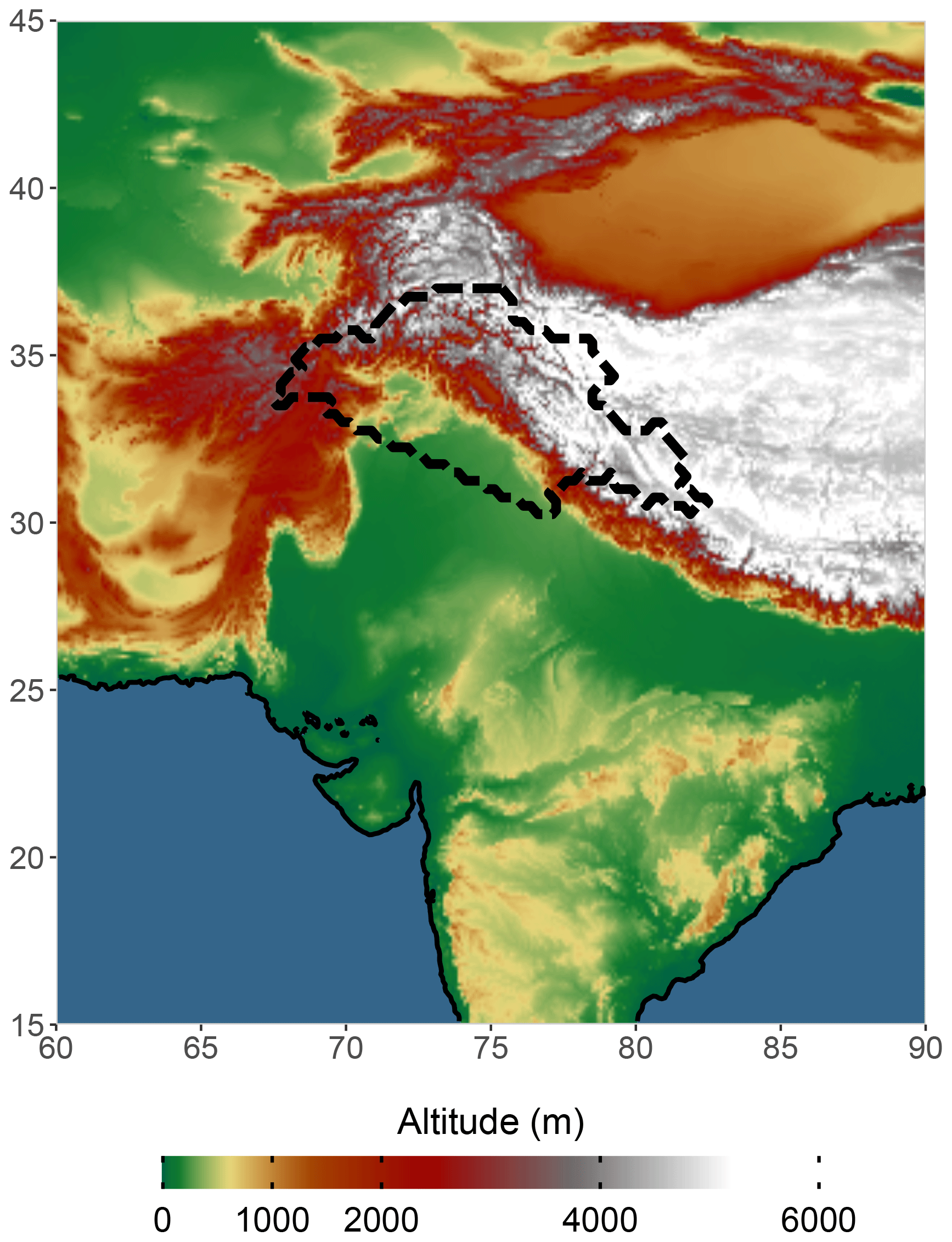
Figure 1Map of the relief of South Asia. The study area (Upper Indus Basin, UIB) is indicated by the dashed line.
3.1 Computing wind and moisture contributions to precipitation
Baudouin et al. (2020a) demonstrated the ability of principal component (PC) regression to analyse the precipitation variability in terms of moisture transport, defined as the product of wind (both components) and specific humidity. A similar method is used here, with small differences, to both simplify and test the robustness of the method. The reasons for each of the changes in the approach and their impact on the coefficient of determination (or explained variance) of the regression are further detailed in Baudouin (2020).
The method uses moisture transport at 700 hPa to predict 3-hourly precipitation between October and May. Moisture transport is considered over an area between 18 and 36∘ N and between 67 and 85∘ E, for a resolution of 0.5∘ (see the extent and resolution in Fig. 2a). The PC analysis is applied on centred time series of moisture transport and considers both meridional and zonal components simultaneously. The first 46 PCs are selected for the regression.2
The prediction of precipitation is a linear combination of the PCs of moisture transport. However, since precipitation can only be positive, negative predictions are fixed to 0. This condition is directly applied to the statistical model of the regression, which is solved using an iterative optimisation method (Brent, 1973). Finally, a condition to correct any bias is also added to the statistical model. The coefficient of regression of this regression is R2=0.878, which is very close to the one found in Baudouin et al. (2020a, R2=0.832).
Figure 2a shows the coefficients of the regression: the arrows are constructed from the coefficients of each component while the colour is proportional to the length of the arrow. The arrows highlight the moisture convergence zone along the Himalayan foothills that triggers precipitation (cf. Baudouin et al., 2020a).
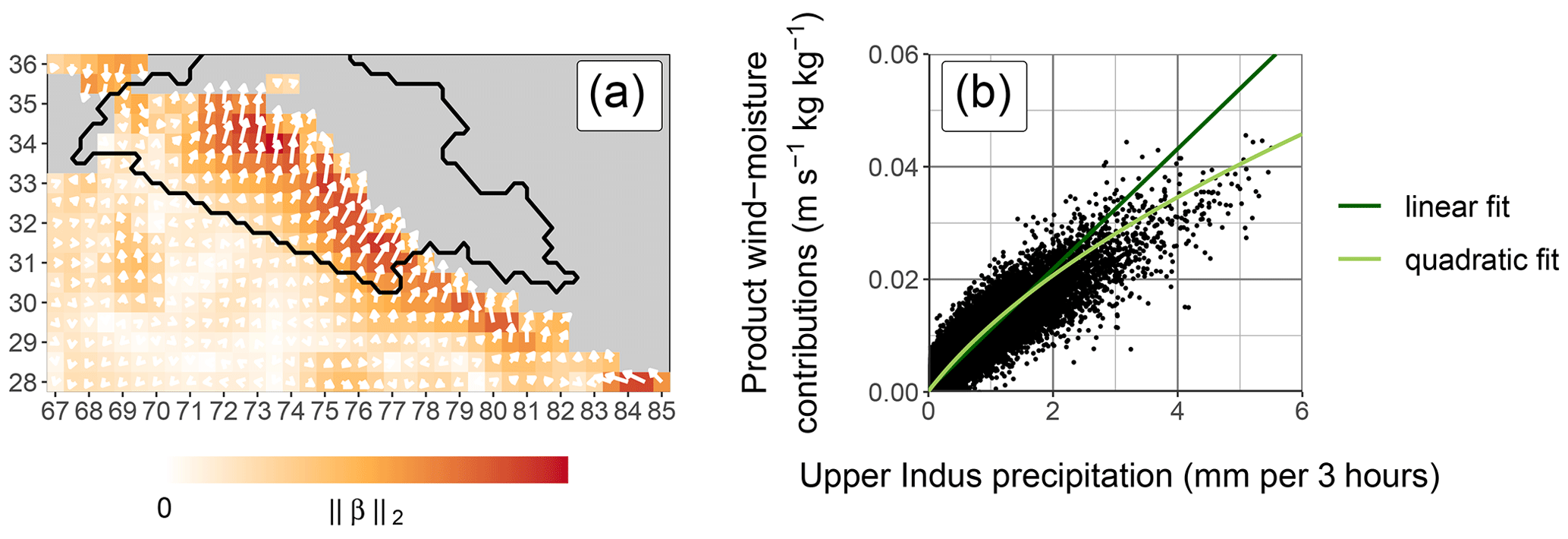
Figure 2Results of the wintertime regression of precipitation with meridional and zonal moisture transport at 700 hPa. Precipitation is defined as the 3-hourly average over the UIB (black contour, panel a). Panel (a) shows the coefficients associated with each predictor. The arrows indicate the most efficient direction of moisture transport while the length and the colour of the arrows indicate the total weight of moisture transport (i.e. the Euclidean norm of the coefficients from both zonal and meridional components). The exact values of the coefficients are not interpretable and are therefore not indicated. Panel (b) is the scatter plot of the product of wind and moisture contributions against precipitation, with the green lines representing two types of fit.
As in Baudouin et al. (2020a), the prediction is split between the contribution of wind and moisture, using a weighted spatial averaging. The wind contribution (labelled hereafter UV700) is computed by multiplying the time series of meridional and zonal wind with the respective meridional and zonal regression coefficients and summing the result. UV700 is interpreted as the cross-barrier wind effect on the precipitation. For the moisture contribution (labelled hereafter Q700), the time series of specific humidity at each location are weighted with the Euclidean norm of the coefficients of both meridional and zonal moisture transport (i.e. the colour scheme used in Fig. 2a). After fixing negative values of UV700 to 0, the product of Q700 and UV700 has an R2 of 0.844 with precipitation, close to the R2 of the regression with moisture transport (0.878), despite the spatial averaging. Note that the intercept of the regression with moisture transport equals 0.14 mm (3 h)−1 but is not taken into account when considering the product of Q700 and UV700.
Figure 2b shows the product of Q700 and UV700 against precipitation. A non-linearity can be seen as precipitation increases more quickly than the product. This non-linearity is not present when including moisture transport at 850 hPa in the PC regression (cf. Baudouin et al., 2020a). This behaviour can be explained by the fact that moisture transport at lower altitude is not proportional to that of higher altitudes and instead quickly increases once strong moisture transport is already present at 700 hPa (Baudouin et al., 2020a). An ad hoc quadratic fit of the precipitation with the product of Q700 and UV700 captures the non-linearity and slightly increases the R2 from 0.844 to 0.853. Hence, the product of Q700 and UV700 is a good predictor of precipitation, and each contribution will be investigated separately in the following sections.
3.2 Relating cross-barrier wind to western disturbances
The second methodological step consists in using UV700 to investigate the link between the cross-barrier wind intensity and various WD characteristics.
First, a qualitative analysis is proposed using a composite. The composite is defined as the average over atmospheric fields of the time steps with the 10 % highest values of UV700 (i.e. 3-hourly UV700 above 2.68 m s−1). This selection of time steps accounts for about 50 % of the precipitation between October and May. To remove the influence of the seasonality, the anomalies of the atmospheric fields are computed by removing the first four harmonics of the seasonal cycle. This approach ensures, for example, that the monthly mean anomalies of geopotential height at 300 hPa are below 10 gpm. Various pressure-level fields are investigated: the geopotential height anomaly at 300 hPa and the anomaly of geopotential thickness between 500 and 300 hPa (Fig. 3), the wind speed and wind speed anomaly at 250 hPa (Fig. 5), the precipitable water anomaly and the absolute water vapour flux (Fig. 10b–g), and the evaporation anomaly and absolute 10 m sea wind (Fig. 11b–d). For a vertical cross-section of the troposphere along 30∘ N (see horizontal white line in Fig. 3a), we also investigate the anomaly of the geopotential height, temperature, specific humidity, and meridional wind (Fig. 4). The section cuts across the Indus Plain between 70 and 78∘ E, just south of the UIB, where the southerly advection originates. In each figure, the lead–lag is relative to the time steps selected for the composite.
For a more quantitative approach, a PC regression is used that is similar to the one developed in the previous section but with different variables. The regression predicts UV700 using 3-hourly time series of three different 2D fields: geopotential height at 300 hPa and geopotential height thickness between 700 and 500 hPa and between 500 and 300 hPa. The predictors are taken within a box between 50 and 90∘ E and between 20 and 50∘ N at 1∘ resolution3 except for the lowest thickness where grid points whose maximal surface pressure is above 700 hPa are removed (see the extent of the colour shading shown in Fig. 6b–d). Both positive and negative values of UV700 are predicted. The time series of the predictors are standardised (i.e. the mean is removed and the result divided by the standard deviation), and the PC decomposition is then performed independently for each 2D field. Finally, the regression makes use of the first 40 PCs of each 2D field, for a total of 120 predictors.
The regression has a high predictive skill, with R2=0.886. The scatter plot of UV700 against its prediction shown in Fig. 6a also suggests that the prediction is successful for a wide range of values of UV700, despite some underestimations for the highest values. The coefficients of the regression are displayed in Fig. 6b–d. The partial prediction of UV700 associated with each of the three fields is called Z300 for the geopotential at 300 hPa, and dZ_UP and dZ_LW for the geopotential thickness between the layers 500 and 700–500 hPa, respectively. Note that a more detailed explanation of the methodology is available in Baudouin et al. (2020a) and Baudouin (2020).
The geopotential height at 300 hPa has been used for tracking analysis (Cannon et al., 2016) and WD indices (Madhura et al., 2015; Midhuna et al., 2020) to characterise WDs. However, only using geopotential heights as predictors limits the predictive skill (R2=0.678) and leads to an underestimation of UV700 for values above 2.5 m s−1 (Baudouin, 2020). This issue is corrected by adding geopotential height thicknesses as predictors. That way, the regression can be interpreted as the decomposition of the wind at 700 hPa into the wind at 300 hPa and the wind shear between the two layers.
We noticed that dZ_UP and dZ_LW are negatively correlated with the predictand UV700. In regression studies, predictors exhibiting such a behaviour are referred to as suppressors: the predictor suppresses the variability in one or several other predictors (Smith et al., 1992; Nathans et al., 2012). In this case, dZ_UP and dZ_LW suppress some of the variability in Z300. To simplify the analysis, a new contribution of the geopotential thickness to the wind is computed. dZa_UP is the residual of the regression of dZ_UP with Z300: the variability in Z300 is removed from dZ_UP. dZa_UP describes the anomalous geopotential thickness given the situation of the geopotential at 300 hPa. The same is performed for dZ_LW. The regression is summarised in the equation below, with as the prediction of UV700:
Note that Z300 is recomputed hereafter so that it includes the fractions a and b derived from dZ_UP and dZ_LW, respectively. Note also the presence of the constant offset β0. The same composites based on the highest value of UV700 as above are used to investigate the evolution of those contributions during a peak of UV700 (Fig. 7).
3.3 Investigating variability in WD structure
There is variability in the dynamic structure of WDs. To investigate this variance, a more complex composite analysis is used, based on two quantile regressions. To maintain comparability with the other composite analysis (cf. Sect. 3.2), the regressions are performed using the time steps whose value of UV700 is above the 90th percentile.4 The quantile regressions predict the first and third quartile of . (see Eq. 1) is preferred to UV700 itself so that the differences between the two subsets are not related to the variability missed by the PC regression of UV700 with geopotential heights and thicknesses. We regress the values of at the selected time steps on several predictors: Z300, the geopotential anomaly at 300 hPa at the centre of the mean WD (36∘ N, 66∘ E), and months. Two subsets are eventually created that include all the time steps whose value of is conditionally below the first (first subset) and above the third (second subset) quartile. These two subsets are used as composite and hereafter referred to as “lower UV700” and “higher UV700”. The properties of the quantile regression ensure that the two composites have the same averaged characteristics regarding the predictors (or conditions) but a mean value of as different as possible. Hence, the inclusion of Z300 and the geopotential anomaly as predictors guarantees that the composite WD in each subset is located at a similar place and has a similar intensity. Months are also included to avoid seasonal biases regarding WD characteristics: for each month, the same number of time steps is present in each subset. Figures 8 and 9 represent the same variables as in Figs. 3 and 5, respectively, but are based on these new composites.
Finally, a second sampling is performed to investigate the specific humidity variability in WDs. Two new subsets (hereafter “low Q700” and “high Q700”) are computed based on two quantile regressions predicting the first and third quartile, respectively, of Q700. We regress the values of Q700 at the same time steps as above. The predictors are the months so as to remove the impact of seasonality and the difference in the geopotential height anomaly between the grid points (36∘ N, 60∘ E) and (36∘ N, 70∘ E). This latter predictor fixes the longitudinal gradient of geopotential across the UIB and, in this way, the position of the composite WD. However, the intensity of the WDs is not fixed as in the previous case. Various composites are derived from these selections: Figs. 12 and 13 comparable to Figs. 10 and 3, respectively.
4.1 WD characteristics
4.1.1 The upper-troposphere disturbance
High UV700 is associated with a negative geopotential anomaly (i.e. cyclonic disturbances) with the minimum located at 36∘ N, 66∘ E, just north of the Hindu Kush, north-west of the UIB (Fig. 3b), and near the tropopause, at around 300 hPa (Fig. 4b), in agreement with previous studies (Hunt et al., 2018a; Midhuna et al., 2020). The lead–lag analysis (Figs. 3b and c, 4a and c) reveals an eastward motion of the disturbance. Both characteristics fit the definition of western disturbances (WDs).
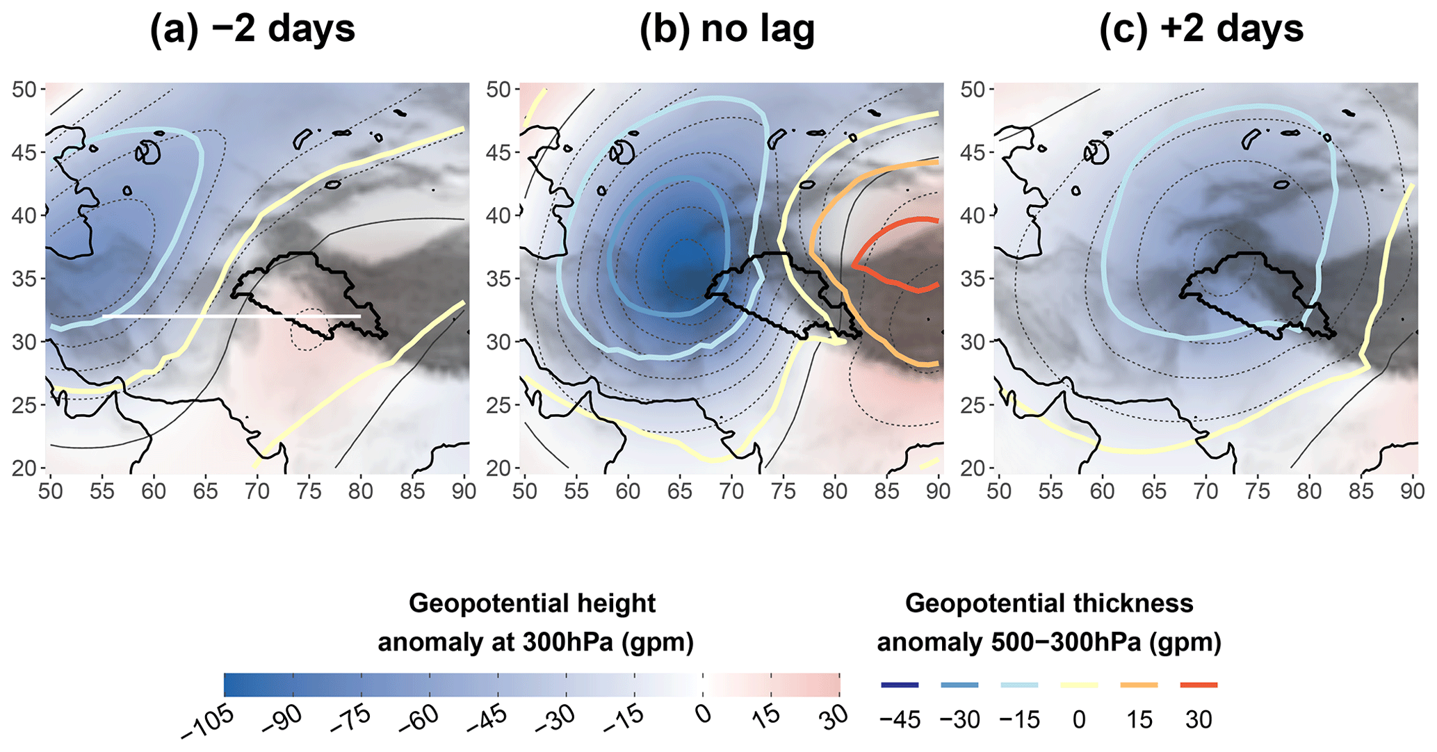
Figure 3Composite maps of a geopotential height anomaly at 300 hPa (colour shading, thin contour lines every 15 gpm) and a geopotential thickness anomaly at 500–300 hPa (thick contour lines). Values are an average based on the 10 % highest values of the 700 hPa wind contribution during winter (UV700, panel b). For panel (a) (panel c) a 2 d lead (lag) is applied to the selection. The white line in panel (a) indicates the cross-section in Fig. 4. The relief (grey shading) and coastline are based on ERA5 data. The UIB is indicated in each panel. Non-significant anomalies at the 95 % level are shown in white (result of a t test on the means). Note that the thickness anomaly is directly indicative of temperature anomalies in that layer under the hydrostatic equilibrium.
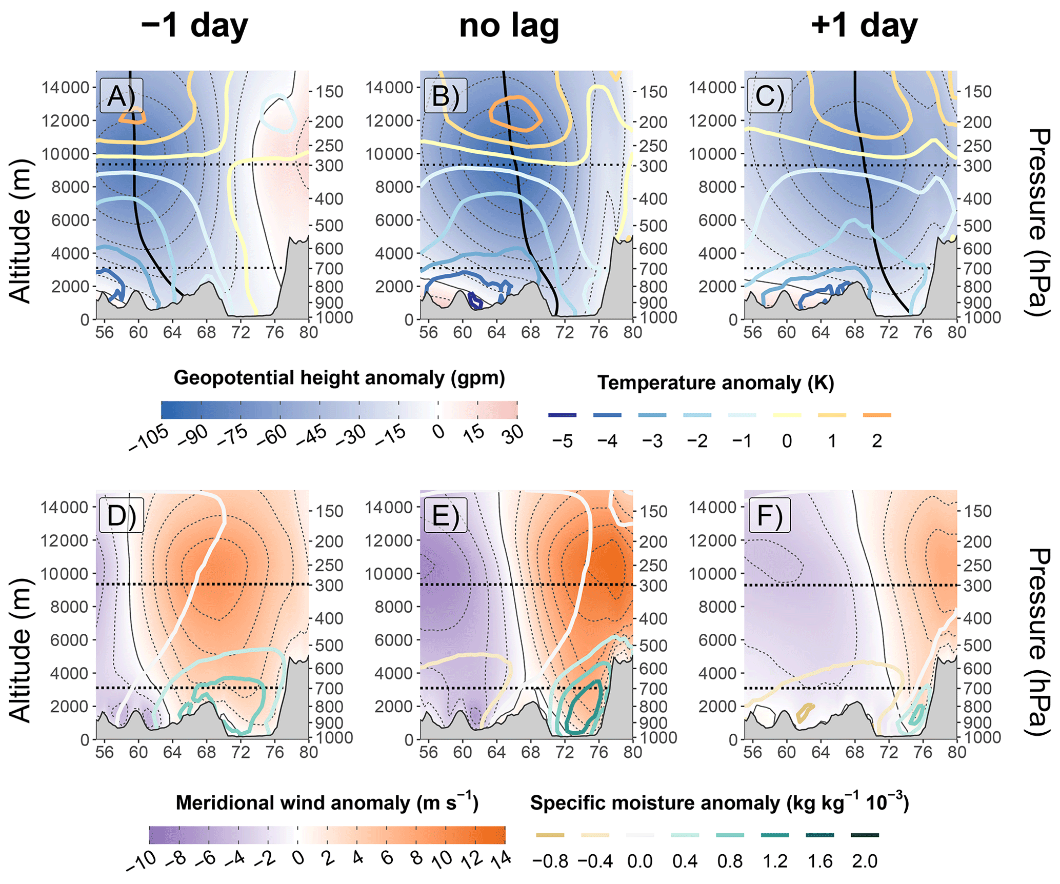
Figure 4Composite cross-section along 30∘ N of the anomaly of geopotential height (colour shading, thin contour lines every 15 gpm) and temperature (thick contour line) in panels (a) to (c) and meridional wind (colour shading, thin contour lines every 2 m s−1) and specific moisture (thick contour line) in panels (d) to (f). Values are an average based on the 10 % highest values of UV700 (b, e). For panels (a) and (d) a 1 d lead is applied to the selection, while a 1 d lag is applied for panels (c) and (f). The dotted horizontal lines represent the levels 700 and 300 hPa, the altitudes for the cross-barrier moisture transport in Fig. 2 and minimum geopotential anomaly in Fig. 3, respectively. The thick vertical black line in (a), (b), and (c) represents the longitude of the minimum geopotential anomaly as a function of altitude. The grey shading represents the relief as in ERA5. Note that the mean meridional wind is close to 0 except near the relief over the Tibetan and Iranian plateaus, where valleys funnel the mean westerly wind.
Interestingly, there is no evidence of a separate cyclonic circulation near the surface, neither on the day of high UV700 (Fig. 4b) nor on the day before (Fig. 4a), as mentioned by Dimri and Chevuturi (2014) and Dimri et al. (2015) among others. Instead, Fig. 4b shows that the lower-altitude circulation is simply a weaker extension of the anomaly at 300 hPa. This downward extension of the cyclonic circulation is also evident in the meridional wind field (Fig. 4d). However, Dimri and Chevuturi (2014) might have referred to fast-moving small-scale eddies that can circulate near the surface of the Indus Plain and are not detected by the composite analysis.
4.1.2 The tropospheric cold core
The weakening of the cyclonic circulation towards the ground is due to a negative temperature anomaly: the WD has a cold core. The centre of the cold core is slightly displaced to the north-west of the geopotential anomaly minimum (Fig. 3b), which indicates baroclinicity. This baroclinicity is even clearer in Fig. 4a–c. There, a vertical black line indicates the location of the maximum anomaly for each altitude and broadly corresponds to the contour of the zero meridional wind anomaly (Fig. 4d–f). The line exhibits a westward tilt with the altitude which is caused by the asymmetry between temperature and geopotential height, a characteristic of the baroclinic structure (Dimri and Chevuturi, 2014; Hunt et al., 2018a). The asymmetry further increases at lower altitude, below 700 hPa, where cold continental dry air is advected from Siberia and Central Asia at the rear of the WD (Fig. 4; Yadav et al., 2012). The Sistan plain in eastern Iran forms a north–south valley between the Hindu Kush and the Iranian Plateau, around 62∘ E in the cross-section, which funnels the cold airflow (Fig. 4b and e). Surprisingly, weaker but still negative temperature anomalies are also present in the Indus Plain, despite the southerly wind bringing in warmer air (Fig. 4b and e). This feature may be related to the adiabatic cooling (i.e. large-scale upward motions) resulting from the baroclinic instability. Closer to the surface, precipitation evaporation and reduced solar radiation could further explain the cooling.
4.1.3 Linking the WDs to the upper-tropospheric wind – jet stream and outflow
WDs are embedded in the subtropical westerly jet (SWJ; Dimri et al., 2015). The SWJ is present in winter at around 250 hPa and between 25 and 35∘ N (see Fig. 5; Schiemann et al., 2009). It exhibits two local maxima independent of WDs: the strongest south of Japan (East Asian jet, above 55 m s−1) and the other between Egypt and Iran (Arabian jet, above 45 m s−1).
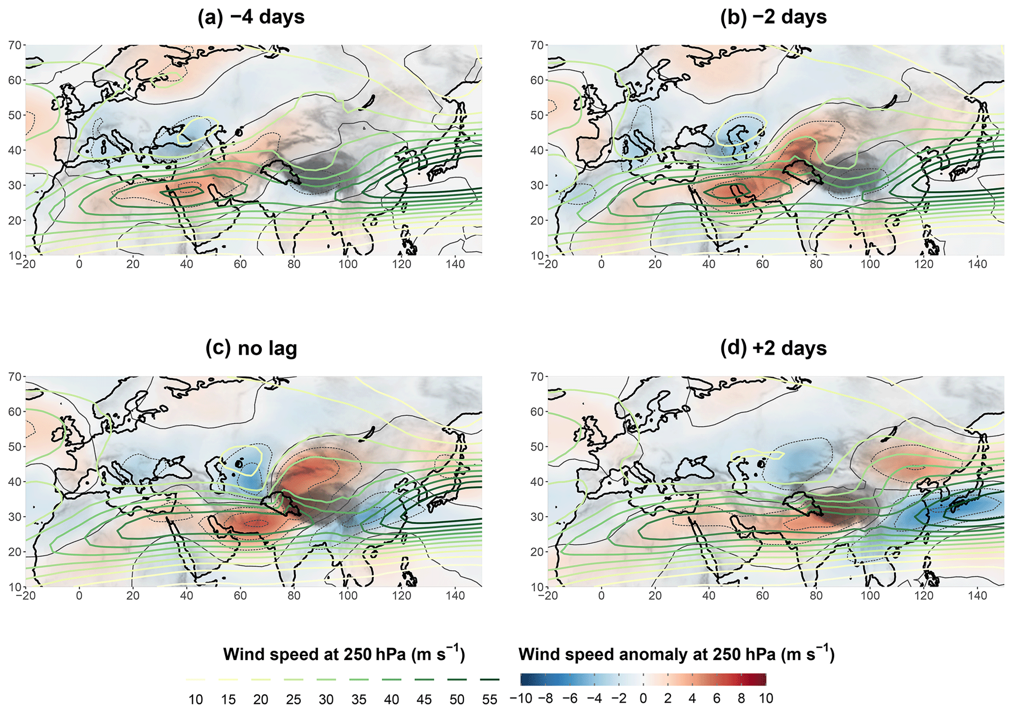
Figure 5Composite maps of wind speed (thick contour lines) and wind speed anomaly (colour shading, thin contour lines every 2 m s−1) at 250 hPa, based, for panel (c), on the same selection of the 10 % highest UV700 as in Fig. 3. For panels (a), (b), and (c), a 4 d lead, a 2 d lead, and a 2 d lag, respectively, is applied to the fields. Non-significant anomalies at the 95 % level are shown in white.
The mean WD centre is located just north of the jet and drives a north–south dipole of the wind speed anomaly that progresses eastwards, following the WD motion (Figs. 3 and 5). The positive wind anomaly results in the narrowing and strengthening of the Arabian jet. Dimri et al. (2015) suggest that part of the strengthening could be due to the merging of the SWJ with the polar jet, which marks the limit between cold and warm air at the surface. This merging is not evident from the Fig. 5, but the composite analysis may hide this dynamic due to the highly variable position of the polar jet. After the peak of UV700, the two parts of the dipole dissociate themselves: the negative northern anomaly slowly moves north-eastwards, while the positive anomaly quickly continues eastwards, south of the Tibetan Plateau, carried by the SWJ (Fig. 5d).
When the lag is negative (Fig. 5a and b), the positive anomaly of wind speed further extends to the north-east, towards Central Asia, outside of the jet core. This deformation corresponds to the second stable position of the SWJ, north of the Tibetan Plateau, which is predominant in summer but may also occur in winter (jet split; Schiemann et al., 2009). A picture from Pisharoty and Desai (1956), still in use in Dimri et al. (2015), suggests on the contrary that stronger wind speed occurs at altitude at the rear of a WD. While some WDs may have this characteristic, WDs triggering high UV700 and thus high precipitation do not exhibit that feature.
As the WD approaches the Tibetan Plateau, a second maximum positive anomaly of wind speed becomes evident over the high elevations: first over the Pamir range (Fig. 5b) and then along the Himalayas (Fig. 5c and d). This anomaly is in part the result of the increased funnelling of the jet over the high ground. At maximum UV700, this positive anomaly extends to the north-east of the WD and corresponds to the outflow of the cross-barrier wind in the UIB. The outflow is characterised by a swift anticyclonic turn, with strong similarity to the warm conveyor belt associated with mature baroclinic waves (Martínez-Alvarado et al., 2014). The increase in latitude and the latent heat release are both key to explaining that change in relative vorticity (Grams et al., 2011). The outflow can also be revealed by the analysis of the cloud cover and the development of a large bank of cirrus (Agnihotri and Singh, 1982; Rakesh et al., 2009; Hunt et al., 2018a).
Finally, after the peak of UV700, the positive anomaly of wind speed related to the outflow completely splits from the circulation associated with the WD and continues eastwards, north of the East Asian jet. By contrast, the WD–relief interaction contributes to lowering the intensity of the SWJ downwind; the East Asian jet is notably weakened as a result (Fig. 5d). Meanwhile, the Arabian jet remains anomalously strong; in fact, 2 d after the peak of UV700 the strength of the anomaly is about the same as 4 d before the peak. Hence, the increased intensity of the Arabian jet is a longer-term feature that seems to promote the intensity or occurrence of a WD but is not directly affected by the passing of one. This feature is evident from several intra-seasonal and inter-annual studies (Filippi et al., 2014; Hunt et al., 2018a; Ahmed et al., 2019). Hunt et al. (2018a) also discussed the influence of the SWJ position on WDs, but the synoptic analysis presented here does not indicate that WDs are related to a change in the position of the Arabian jet.
4.2 Explaining UV700 variability using the PC regression
4.2.1 Interpretation of the PC regression
The results of the PC regression developed in Sect. 3.2 are presented using Fig. 6. Two patterns are distinguishable in the coefficients for Z300 (Fig. 6b). The first is a dipole across the UIB, indicative of a geopotential gradient, which translates into a south-westerly geostrophic wind for positive UV700. The second, less clear, is a ring of positive coefficients around the negative centre of the dipole. The related gradient indicates a cyclonic anomaly for positive UV700 and therefore a WD. The extent of the ring can be interpreted as the effective radius of the centre of the anomaly in triggering a cross-barrier wind in the UIB. The centre of the pattern is located to the west of the study area, where the relief forms a notch important to triggering the vertical velocities (see Fig. 1 in Baudouin et al., 2020a; see also Lang and Barros, 2004; Cannon et al., 2015). In conclusion, Z300 is representative of a cyclonic south-westerly geostrophic wind at 300 hPa.
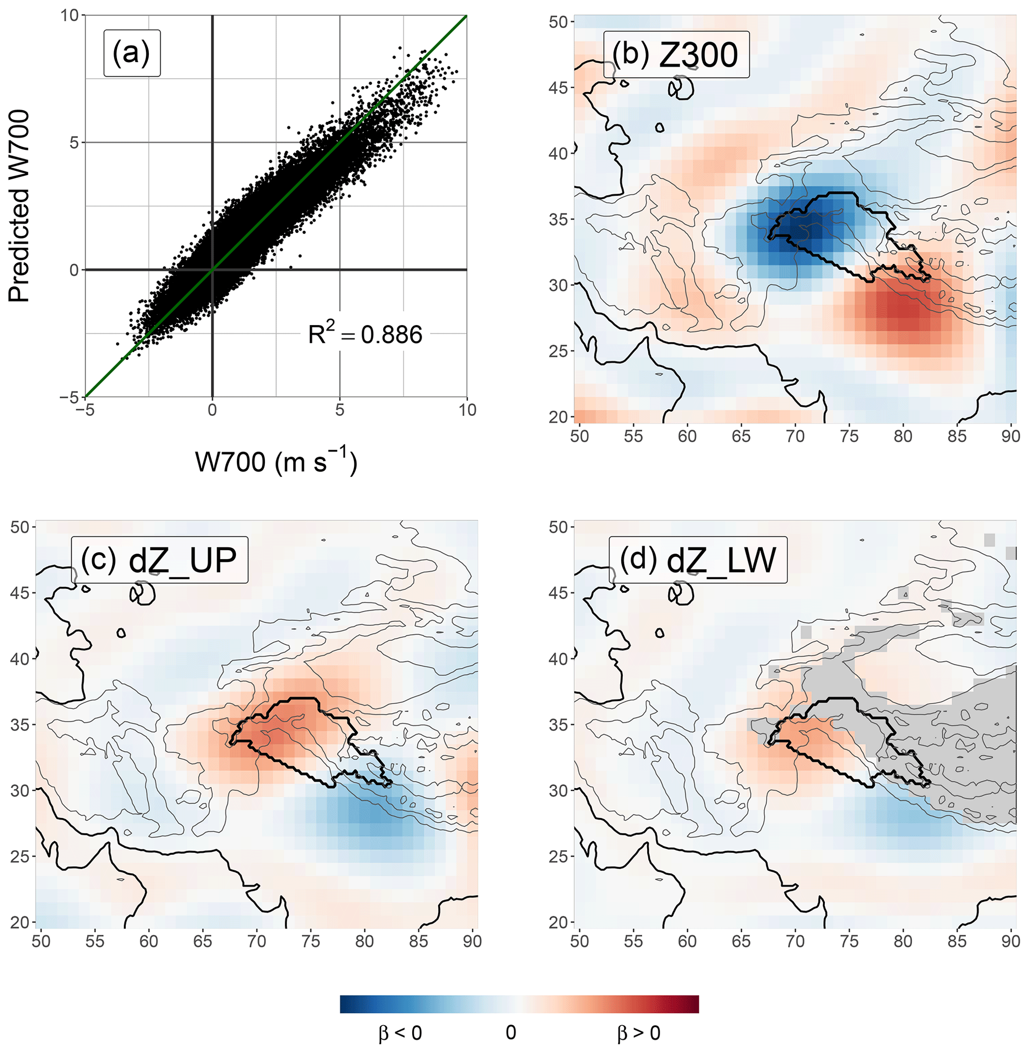
Figure 6Results of the regression of 3-hourly UV700 with geopotential height at 300 hPa (Z300), geopotential thickness 500–300 hPa (dZ_UP), and geopotential thickness 700–500 hPa (dZ_LW). Panel (a) is the scatter plot between the predictand and the prediction. Panels (b), (c), and (d) show the coefficients associated with each predictor (cf. Baudouin et al., 2020a, Eq. 5). The exact values of the coefficients are not interpretable and are therefore not indicated.
The coefficients associated with dZ_UP and dZ_LW are very similar and represent a dipole at a similar location to the one discussed for Z300 (Fig. 6c and d). The related gradient is equivalent to a north-easterly thermal wind, that is, an increase in south-westerly wind towards lower altitudes. However, the composite analyses showed that the cyclonic circulation associated with WDs weakens towards lower altitudes (Fig. 4b) and that the southerly wind is weaker closer to the surface (Fig. 4e). Indeed, dZ_UP and dZ_LW are negatively correlated with Z300. The new contributions dZa_UP and dZa_LW are designed so that they do not correlate with Z300 (cf. Sect. 3.2); rather they characterise the thermal structure of the WDs. If dZa_UP or dZa_LW are positive (negative), then the north-west–south-east temperature gradient over the UIB is weaker (stronger) than usual, and, consequently, the cold core of the WD is smoother, weaker, or further away (deeper or closer). These characteristics of the cold core are also evident from the composite maps for different UV700 intensities (Fig. 8b and e). The importance of the thermal structure has been little investigated previously. Midhuna et al. (2020) used geopotential thickness to characterise WD intensity. They suggested that a colder WD (a thinner 850–200 hPa layer) characterises a more intense WD. The analysis here, however, shows on the contrary that a WD with a warmer core than usual (or displaced cold core) produces stronger near-surface dynamics that enhance precipitation.
Interestingly, the patterns for all predictors (Fig. 6b–d) suggest that UV700 is sensitive to a geostrophic wind that is rotated by approximately 45∘ compared to the southerly wind that it is meant to predict (cf. Fig. 2). Although the geopotential gradient is sufficient to predict wind intensity, it does not indicate the wind direction, which bends towards the lower pressures, as noted in Baudouin et al. (2020a). In this paper, it is suggested that this ageostrophic effect is caused by the drag along the Himalayan barrier and that it is key to trapping the cross-barrier flow in the notch formed at the intersection between the Himalayas and the Hindu Kush.
Finally, the regression successfully predicts the negative values of UV700 (Fig. 6a). These correspond to northerly divergent winds at 700 hPa in the UIB. The regression suggests that they are related to anticyclonic north-easterly geostrophic winds. Since these winds are much less common than their south-westerly counterparts, large negative values of UV700 are rarer than positive ones. The regression also slightly underestimates the highest values of UV700, possibly because the larger latent heat release and increased buoyancy in the context of stronger convergence further sustain cross-barrier winds before the pressure gradient can adjust to them.
4.2.2 Evolution of the partial predictions
The different partial predictions of UV700 vary during a wind peak event as is evident in Fig. 7. The peak value of UV700 (i.e. at no lag) is first due to dZa_UP (accounting for 46 % of the predicted value), highlighting the importance of considering the WD thermal structure. Z300 is close behind (43 %), while dZa_LW has a minor role (11 %). Interestingly, UV700 (the dashed orange line) rises and decays symmetrically around its peak. However, this is not the case for its different partial predictions (other dashed lines). All partial predictions rise steadily before the wind peak. However, the two partial predictions associated with geopotential thicknesses peak before UV700 reaches its maximum intensity and quickly drop after: UV700 is only maintained by Z300 after its peak. The asymmetry between Z300 and dZa_UP can be investigated with Figs. 3 and 4. Focusing on Fig. 3a, 2 d before the wind peak, a gradient in geopotential is already present over the UIB in relation to the positive geopotential anomaly ahead of the WD (increasing Z300). This gradient is indicative of a southerly advection and a warm anomaly that limits the presence of any gradient in temperature (increasing dZa_UP). At the wind peak (Fig. 3b), the approaching WD tightens the gradient of the 300 hPa geopotential while the colder air remains at the edge of the UIB (peak of both Z300 and dZa_UP contributions). The WD enters the UIB with its cold core 2 d after the wind peak at 700 hPa (Fig. 3c). The geopotential gradient remains tight, but the increased temperature gradient counterbalances it, so the southerly wind at 700 hPa weakens (Z300 remains high, but dZa_UP quickly decreases).

Figure 7Lead/lag composite around the 10 % highest values of UV700, as in Figs. 3, 4, and 5, for ERA5 precipitation, contributions to precipitation based on moisture transport (UV700, Q700; see Sect. 3.1), and partial prediction of UV700 based on geopotential (Z300) and the geopotential thicknesses anomaly (dZa_UP and dZa_LW; see Sect. 3.2). Note that Z300, dZa_UP, and dZa_LW have the same units as UV700 and, with the intercept, add up to the prediction of UV700 ; see Eq. 1).
4.3 Geostrophic processes and baroclinic interaction
4.3.1 Importance of the upper-troposphere geopotential gradient
The PC regression indicates that the presence of an east–west geopotential gradient across the UIB is more important for the cross-barrier wind than the proximity of a WD, as long as it remains upstream of the UIB (Fig. 6b). The importance of this gradient is confirmed by the presence of a positive geopotential anomaly over the Tibetan Plateau during high-UV700 events (Fig. 3b). The intensity of this anomaly is also clearly coupled with that of UV700 (Fig. 8b and e).
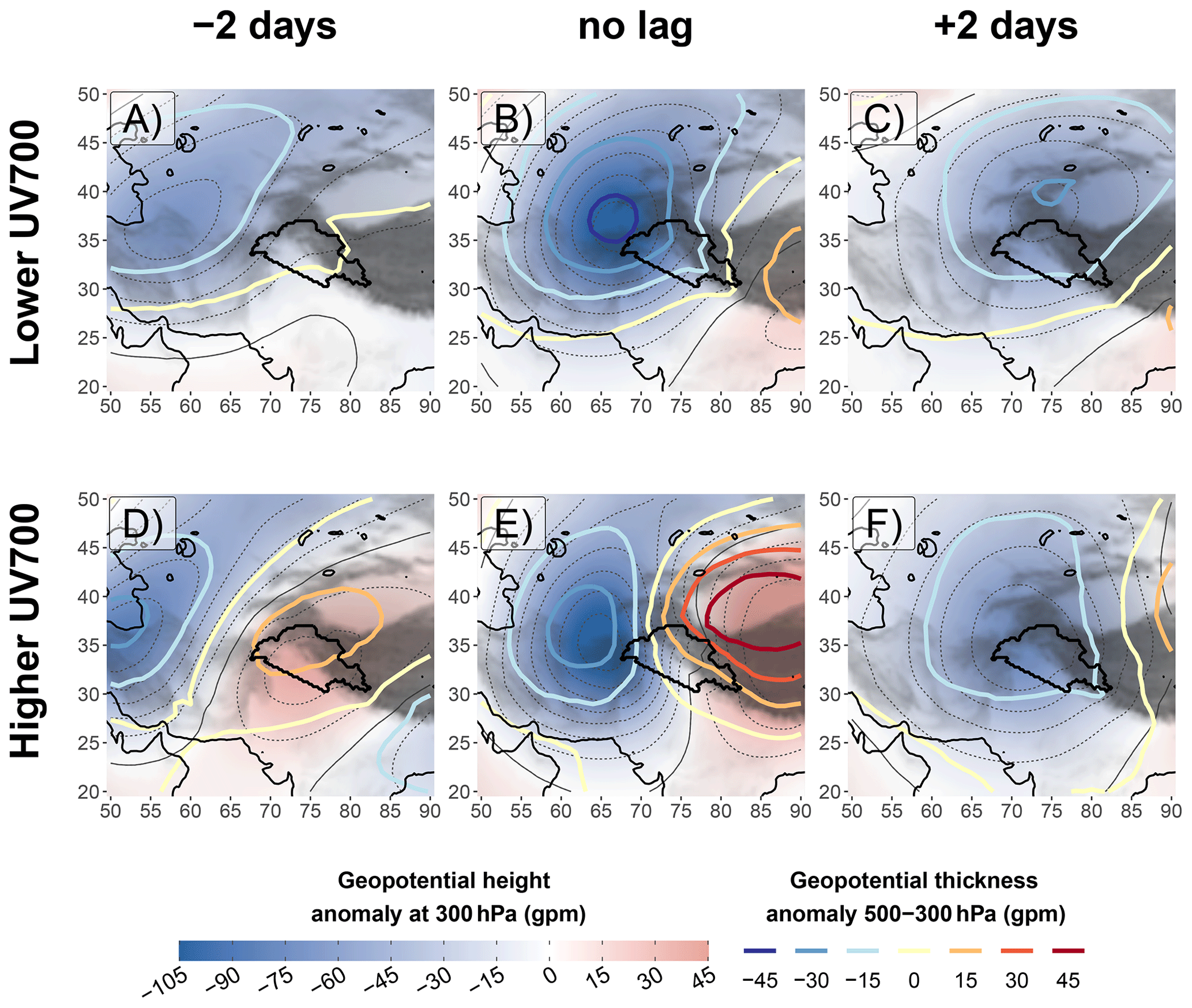
Figure 8Same as Fig. 3, but the composites are based on a subsampling of lower (higher) values of UV700 while still being above the 90th percentile, in panels (a) to (c) (d to f). The subsampling is made so that it is not impacted by seasonality or by the intensity of the WD (see Sect. 3.3). This way, comparisons can be made with Fig. 3.
This anticyclonic anomaly is already present over the UIB 2 d before the wind peak (Fig. 3a) and in conjunction with the WD forms a wave train that has already been discussed in the literature (Dimri, 2013; Hunt et al., 2018b). However, these previous studies have not stressed the importance of this anticyclonic extreme, which increases the zonal gradient of geopotential to the east of the WD and thus strengthens the southerly wind. The downward propagation of that gradient of pressure is sufficient to trigger the cross-barrier meridional flow. In fact, the zonal gradient is already present at 700 hPa 1 d before the wind peak, despite the mean WD centre being located at about 1500 km to the west, owing to the tilt of the circulation and the presence of positive geopotential anomalies towards the Himalayas. Hence, cross-barrier wind and precipitation can all occur well ahead of a WD. By contrast, when the WD is above the UIB, the zonal gradient of geopotential at 700 hPa disappears, stopping the cross-barrier meridional flow (Fig. 4c and f).
4.3.2 Changes in WD motion speed
The speed of the mean WD can be calculated using the lead–lag analysis: the centre moves by 13∘ of longitude in 2 d between Fig. 3a and b, indicating a mean speed of about 6.8 m s−1, which is not far from the phase velocity of 5 m s−1 found in Hunt et al. (2018b) but is slower than the 8 to 10∘ d−1 found in Datta and Gupta (1967) (see Dimri et al., 2015). Interestingly, Fig. 3c shows a slowing of the mean WD to about 3.1 m s−1, although the composite method limits the analysis in terms of mean speed of the WDs. Slower or even static cyclonic circulation on the surface is sometimes discussed in the literature (e.g. Lang and Barros, 2004; Dimri and Chevuturi, 2014) but not the slowing of the tropopause disturbance itself.
The speed of the WD is also different depending on whether higher or lower UV700 is considered (Fig. 8). Before the peak of UV700, the WD is moving significantly faster in the group with the highest peak values of UV700 (6.8 m s−1, Fig. 8d and e) than in the other group (4.2 m s−1, Fig. 8a and b). This change in translation speed does not seem to be related to a change in the 250 hPa wind speed (Fig. 9). We rather suggest it to be related to a difference in the mechanisms explaining the development of the wave supporting the WD.

In the lower-UV700 case, the development of the WD is accompanied by the reinforcement of the cold anomaly (Fig. 8a and b), suggesting that the tropopause anomaly mostly grows from the equatorward motion of cold air at the rear of the WD. This growing process results in a steady upwind propagation of the wave. By contrast, the temperature anomaly does not change as the WD with higher UV700 approaches the UIB and strengthens (Fig. 8d and e). In this case, the WD does not grow but propagates faster.
Furthermore, a stronger cross-barrier wind results in a more severe slowing of the WD. After the peak of UV700, the WD with higher UV700 slows to 3.2 m s−1 (Fig. 8e and f), even slower than the WD with lower UV700 (3.8 m s−1, Fig. 8b and c). The intensifying uplift in the UIB during an event of high cross-barrier winds increases the near-tropopause convergence over the UIB (cf. quadrupole of divergence field in Hunt et al., 2018a). This convergence zone results in the decay of the WD from its east and therefore the WD's slowing. This process corresponds to the last and decaying stage of a baroclinic interaction, which is now further investigated.
4.3.3 Thermal structure feedback
A first simple way to describe the baroclinic interaction at play in the UIB is through the feedback between circulation and thermal structure. The analysis of the PC regression reveals the importance of the horizontal temperature gradient at 300 hPa and how a displaced or weaker cold core enhances the circulation at 700 hPa. Yet, the southerly wind east of the WD brings warm air to the Indus Plain at all altitudes (Fig. 4), depending on the large-scale north–south temperature gradient. This flow therefore contributes to displacing the cold core of the WD to the west of its circulation centre at the tropopause and to reinforcing the 700 hPa circulation in the Indus. The Iranian Plateau and the Hindu Kush act as a barrier to the arrival of the cold air from the north-west, while the flat Indus Plain channels the southerly wind, further enhancing the positive feedback process.
At a local scale, the UIB is a hotspot where most of the near-surface convergence occurs. There, warm advection, latent heat release, and mixing prevent the cold air from extending into the UIB as the WD progresses eastwards. The tropospheric zonal temperature gradient is therefore reduced, which in turn increases the geopotential height gradient at 700 hPa and thus the cross-barrier wind and the uplift (see analysis of the PC regression). This effect explains the general potential for intense cross-barrier winds in the area. The cold core eventually enters the UIB when the cold air invades the Indus Plain to the south of the UIB and stops the advection of warm air.
4.3.4 Ageostrophic circulation induced by baroclinicity
Baroclinic interaction can also be described using quasi-geostrophic theory and potential vorticity (PV). When a positive PV anomaly evolves in a sheared environment, baroclinically forced vertical velocities occur: uplift upwind of the anomaly and subsidence downwind (Malardel, 2005). More specifically, it is the zonal gradient of PV ahead of (behind) the PV anomaly that triggers the baroclinic uplift (subsidence). A baroclinic interaction occurs when a surface and a tropopause anomaly align such that the vertical velocities associated with one enhance the other anomaly by stretching it. The two disturbances grow and their associated vertical velocities increase until the shear leads to the spatial dephasing of the disturbances. Then, a reverse negative feedback process takes place, leading to the quick decay of both disturbances. These processes characterise the most intense cyclonic activity (Malardel, 2005; Dacre et al., 2012).
A WD is characterised by a high PV anomaly (Hunt et al., 2018a), and the SWJ in which it is embedded provides the shear needed to produce the vertical velocities. This process has already been suggested as a key factor in explaining vertical velocities in the UIB (Sankar and Babu, 2020) or the interaction with tropical depressions (Hunt et al., 2021). However, as discussed earlier (Sect. 4.1.1), there is no evidence of a near-surface disturbance that would trigger a baroclinic interaction. This has led Hunt et al. (2018a) to describe WDs as “immature baroclinic waves”. We further suggest that the relief and the orographic uplift provide the low-altitude feedbacks for a similar, yet short-lived, baroclinic interaction.
The zonal gradient of PV upwind of the WD triggers a baroclinic uplift to the east of the anomaly. As the WD approaches the UIB, its interaction with the relief results in an orographic uplift, which combines with the baroclinic uplift. However, the uplift also results in decreased PV at high altitude (300 hPa) over the UIB due to the advection of lower tropospheric PV as well as diabatic heating. Hence, the zonal PV gradient increases and stronger baroclinic uplift occurs, resulting in a positive feedback. Once the high-PV anomaly associated with the WD enters the UIB, the mechanism reverses: the orographic uplift results in the weakening of the PV anomaly, eventually leading to the decay of the WD.
The input of low PV at high altitude from the UIB is evident from the anticyclonic turn of the outflow (see discussion on Fig. 5c in Sect. 4.1.3) and from the warm area at 300 hPa to the east of the WD but largely displaced compared to the geopotential anomaly maximum (Fig. 3b). Moreover, the baroclinic interaction and the intense uplift are revealed by the deformation of the jet near the UIB during the passing of the WD (Fig. 5). Particularly, when the uplift is maximal, the jet configuration is characteristic of a strong divergence at the tropopause over the UIB: the study area is located near the eastern exit of the Arabian jet and in the right entrance of the outflow.5 This mechanism is similar to the baroclinic interaction between a tropopause anomaly and a surface disturbance but where the surface disturbance is replaced by the relief. It also results in a weaker, shorter-lived interaction.
The different thermal structures shown in Fig. 8 are linked to a difference in the strength of baroclinic processes. This difference becomes evident when looking at the wind at 250 hPa. In the case of higher UV700 (Fig. 9b), the pattern of the wind anomaly is very similar to in Fig. 5c. The outflow is more intense and clearly detached from the anomalously strong SWJ. By contrast, in the case of lower UV700 (Fig. 9a), the anomalously strong SWJ extends to the south-east of the UIB and forms a diffluence over the Tibetan Plateau while there is no evidence of a distinct outflow. In that context, the UIB is no longer located in a tropopause divergence configuration.
To conclude, WDs are a prerequisite to cross-barrier winds in the UIB. Both the strength of the 300 hPa low and its baroclinic context are important for the cross-barrier wind intensity. In the composites in Fig. 8, UV700 is two-thirds higher in the higher case (5.3 m s−1) than in the lower case (3.2 m s−1), a difference mostly explained by the difference in baroclinicity. However, the increase in precipitation is almost 3-fold, from 5.9 to 16.8 mm (3 h)−1. This difference is partially explained by the quadratic fit (see Fig. 2b) but also by a change in moisture supply (Q700), from kg kg−1 to kg kg−1, which is now further investigated.
5.1 General
The UIB and the Indus Plain are dominated by a mean westerly moisture flux during the season of active WDs (Fig. 10a). However, precipitable water is over 15 mm in the Indus Plain, while it is below 10 mm to the west of the plain, in relation to the higher elevations (e.g. Sulaiman Range, Hindu Kush, Iranian Plateau). This being the case, transient circulation or local evaporation is needed to explain the higher amount in the plain. Furthermore, the moisture content (and moisture contribution, Q700) rises during a peak of UV700 and in the days before as shown in Figs. 4d and e and 7, indicating the importance of WDs in moisture variability. Therefore, to understand the origin of, pathway of, and variability in the moisture that eventually precipitates, the moisture flux needs to be investigated during the passing of a WD.
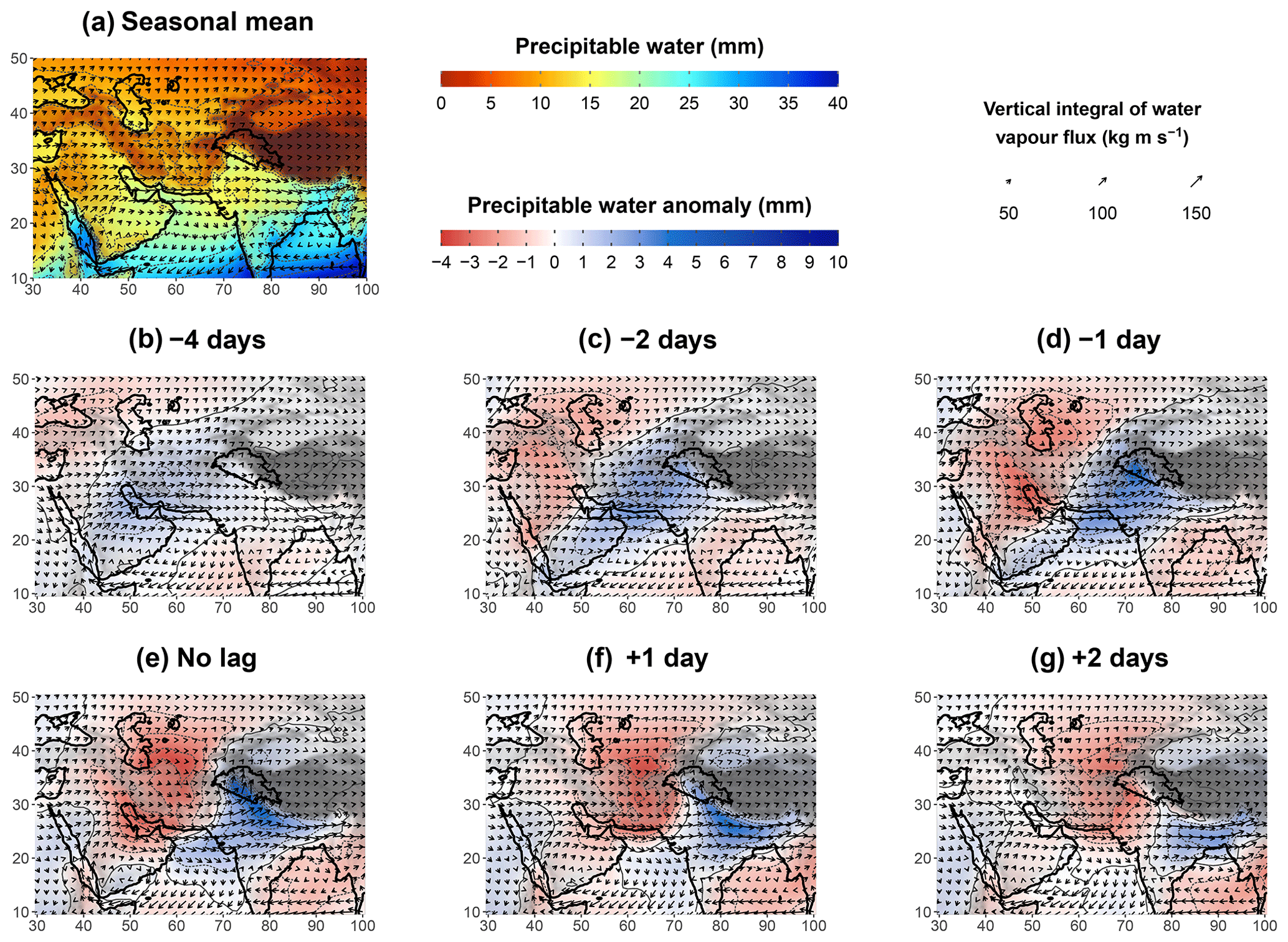
Figure 10(a) The seasonal mean of precipitable water (colour shading, thin contour lines every 5 mm) and vertical integral of water vapour flux (arrows). The mean is weighted by the seasonality of the occurrence of UV700 above its 90th percentile. Panels (b) to (g) show the lead–lag composite maps, with respect to the 10 % highest values of UV700 (as in Fig. 3), of the precipitable water anomaly (colour shading, thin contour lines every 2 mm) and absolute water vapour flux (arrows). Non-significant anomalies at the 95 % level are shown in white.
5.2 Moisture pathway to the UIB
Figure 10e shows a significant accumulation of precipitable water in the UIB when UV700 is maximal: the anomaly represents an increase of 30 % to 50 % in precipitable water in the UIB compared to the mean. The anomaly extends along the Himalayas, towards north-east India, as well as towards the Arabian Sea. Hunt et al. (2018b) found a similar pattern when investigating extreme precipitation events. This relationship between wind and precipitable water is first explained by the near-surface moisture convergence induced by the cross-barrier wind, particularly near the foothills. However, composites of negative lags in Fig. 10b–d suggest that anomalously wet air masses advected into the UIB are also responsible for the increase in precipitable water.
Moisture had already been building up over the Persian Gulf 4 d before the peak of UV700 (Fig. 10b). The direction of moisture transport indicates that this moisture is advected from the Red Sea across the Arabian Peninsula. This transport, as well as how it is enhanced by Mediterranean lows, is described in Chakraborty et al. (2006) and Mujumdar (2006). This moisture flow passes over the coastal mountain ranges along the Red Sea (Sarawat Mountains, with peak heights ranging from 1000 to 3000 m). The moisture is therefore present at a relatively high altitude, similar to that of the cross-barrier wind in the UIB (700 hPa). The more intense wind at this altitude rather than closer to the surface has the potential to quickly transport the moisture towards the study area.
The positive anomaly of precipitable water has spread from the north side of the Arabian Sea to the Indus Plain and the mountains to the west 2 d later (Fig. 10d). The south-westerly moisture flux clearly suggests that air masses from the north of the Arabian Sea and the Persian Gulf contribute to the increase in precipitable water, as mentioned by Hunt et al. (2018b). Moisture convergence over the windward side of the mountains also helps to increase moisture at higher altitudes as can be seen over the Sulaiman Range, 1 d before the peak in Fig. 4d. Convergence also starts over the UIB, more specifically in the notch formed by the mountain ranges, 1 d before the peak of UV700, resulting in a maximum of the precipitable water anomaly (Fig. 10d).
This analysis shows the existence of a pathway of moisture that sustains moisture content in the UIB. It originates from the Red Sea, crosses the Arabian Peninsula towards the Persian Gulf, continues towards the north of the Arabian Sea and the Indus Plain, and ends in the UIB. Previous studies have implied the existence of such a pathway without investigating it further (Filippi et al., 2014; Hunt et al., 2018b; Ahmed et al., 2019). Part of this circulation, from the Red Sea to the Arabian Sea, is visible in the seasonal mean (Fig. 10a) and is driven by the subtropical gyre located on the south-eastern tip of the Arabian Peninsula. WDs strengthen this flow as suggested in Hunt and Dimri (2021) but most importantly steer it towards the UIB. In some extreme cases, this moisture pathway can form atmospheric rivers (cf. Bao et al., 2006; Zhu and Newell, 1998) that are related to extreme precipitation events along the Himalayas (Thapa et al., 2018). This analysis also suggests that neither the Mediterranean Sea nor the Caspian Sea is an important contributor of moisture for the precipitation in the UIB, in agreement with Jeelani et al. (2018) and Dar et al. (2021).
5.3 Evaporation sources
The local evaporation in the UIB is quite high compared to the surrounding land, about 1 to 2 mm d−1 (Fig. 11a), and is little affected by the passing of a WD (Fig. 11c). While this process helps sustain the generally higher precipitable water in the UIB, it cannot explain the precipitable water anomaly associated with a WD. The rest of the Indus Plain, as well as the nearby mountains, contributes very little to the moisture, as those areas are arid, and the wetter and higher ground is too cold in winter to generate significant evaporation.
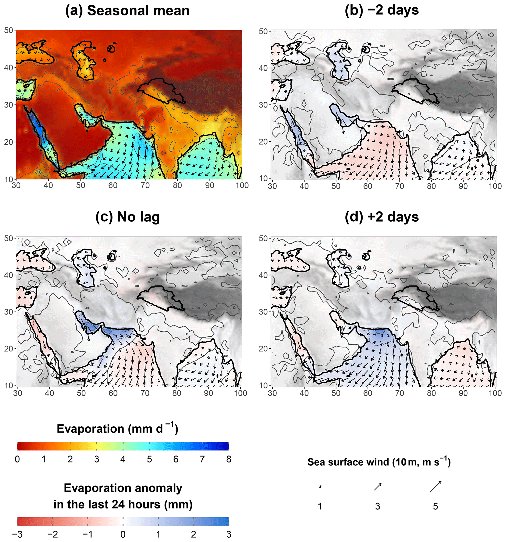
Figure 11Panel (a) is similar to Fig. 10a but for evaporation (colour shading, thin contour lines every 5 mm) and 10 m sea winds (arrows). Panels (b) to (d) are similar to Fig. 10c, e, and g but for cumulated evaporation in the last 24 h before the peak of UV700 plus the lead or lag indicated (colour shading, thin contour lines every 2 mm) and 10 m sea winds (arrows).
The mean evaporation rate over the Persian Gulf and the north Arabian Sea is about 4 to 5 mm d−1 (Fig. 10a). That is, a day of evaporation represents a quarter of the total precipitable water in the area. This high replacement rate suggests that a large amount of the moisture arises from those water bodies directly, and it also emphasises the importance of the persistence of the moisture pathway between the two to build up moisture content. Even stronger evaporation rates are present in the Red Sea, particularly to the north. As mentioned earlier, despite the distance, the Red Sea seems important for increasing moisture at higher altitudes so that the moisture can be more easily transported.
These two composite analyses clearly identify the north of the Arabian Sea, the Persian Gulf, and the Red Sea as the main sources of moisture for the precipitation in the UIB for the first time. However, this approach does not allow for any quantification, nor does it discuss variability. A more complex analysis involving numerical tracking would be needed, and that is beyond the scope of this study.
5.4 Other impacts of the passing of WDs on the moisture field
WDs impact the intensity and end point of the moisture pathway (Sect. 5.2), but other impacts are evident from Figs. 10 and 11 as well. A negative anomaly of precipitable water propagates from the Tigris–Euphrates plain into the Persian Gulf 2 d before the peak of UV700 (Fig. 10c) and reduces the moisture supply from the Red Sea. This circulation is the result of a surge of surface, cold, and dry air at the rear of WDs. The negative anomaly eventually propagates to the north of the Arabian Sea after the peak of UV700 (Fig. 10e–g) but tends to weaken. This weakening can be explained by the large evaporation anomaly present over the seas as the dry air progresses (Fig. 11b–d). Evaporation rates almost double compared to the seasonal mean (Fig. 11a), which is enough to eliminate the precipitable water anomaly in a day. This evaporation anomaly can be explained by both the increase in surface wind speed induced by the WD (arrows in Fig. 11) and the very low surface dew point of the air blown from the land.
A second but connected area of a negative anomaly of precipitable water is present over Central Asia and the Caspian Sea (Fig. 10c and d). It also relates to cold and dry air being advected by the WD from northern latitudes. When UV700 peaks, this cold and dry air mass invades the mountains to the west of the Indus Plain (Fig. 10e; see also Fig. 4b and d). Unlike the other air masses that are advected over the sea, the encounter with the relief further increases the moisture anomaly through a Foehn effect. This effect is strongest after the peak of UV700, as the mean moisture flux over the Indus Plain veers eastwards. The continental dry air descends from the Sulaiman Range and the Hindu Kush, replacing the maritime moist air (Fig. 10f and g). As the UIB is cut from its moisture supply, the precipitable water anomaly becomes negative (Fig. 10g), which severely limits moisture transport and precipitation despite the continued presence of a cross-barrier wind. Similarly, Fig. 7 indicates that the passing of a WD noticeably reduces Q700 several days after the peak of UV700.
Hence, a WD has two opposite effects on moisture content in the UIB: moistening before its passing and drying afterwards. Therefore, another ensuing WD may be inhibited, in terms of precipitation, by the dryer conditions dominating in the Indus Plain and the UIB, suggesting a negative feedback effect. However, one could also imagine a positive feedback, where a quick succession of WDs provides a continuous moisture supply from the maritime sources by inhibiting the dry air invasion. The interaction between WDs is not further investigated here and is likely subject to high variability and dependent on larger- and smaller-scale atmospheric circulation.
After the peak of UV700, the positive anomaly of precipitable water moves along the Himalayas towards north-east India where it enhances cross-barrier moisture transport and orographic precipitation in another notch that is formed by the relief, enhancing orographic precipitation there. The impact of WDs is not as evident in this area, first because the tropopause disturbances have mostly disappeared due to the interaction with the relief in the UIB and secondly because convection is a more important driver of precipitation (Tinmaker and Ali, 2012; Mahanta et al., 2013; Mannan et al., 2017).
Finally, the north-easterly trade winds that blow over most of the Arabian Sea are also affected by WDs: they are weaker ahead of the WD, leading to a decreased evaporation (Fig. 11b), which also slightly decreases precipitable water along 10∘ N (Fig. 10b to e). However, trade winds intensify after the passing of the WD, thus increasing evaporation (Fig. 11d) and leading to a slight increase in precipitable water to the south (Fig. 10f and g).
5.5 Impact of WD characteristics on Q700
Various WD characteristics influence moisture contribution (Q700). There exists a direct link between UV700 and Q700: their peak is concurrent as a WD passes (Fig. 7), and their correlation reaches 0.45 for the entire winter season (once the seasonal mean is removed from Q700). This relationship is explained by the advection of moisture by the cross-barrier wind from both the south (from the moisture pathway) and the near surface (due to uplifting). Since the intensity and the thermal structure of a WD at 300 hPa impact UV700 (see Sect. 4.2), they also impact Q700. However, the shape and direction of a WD have an even greater impact by acting on the balance between the supply of maritime moist air and the intrusion of continental dry air discussed earlier (Sect. 5.4). This impact is investigated using the results of the second quantile regression described in Sect. 3.3 and composite maps over two selections, one representative of low Q700 and the other of high Q700 (Figs. 12 and 13).

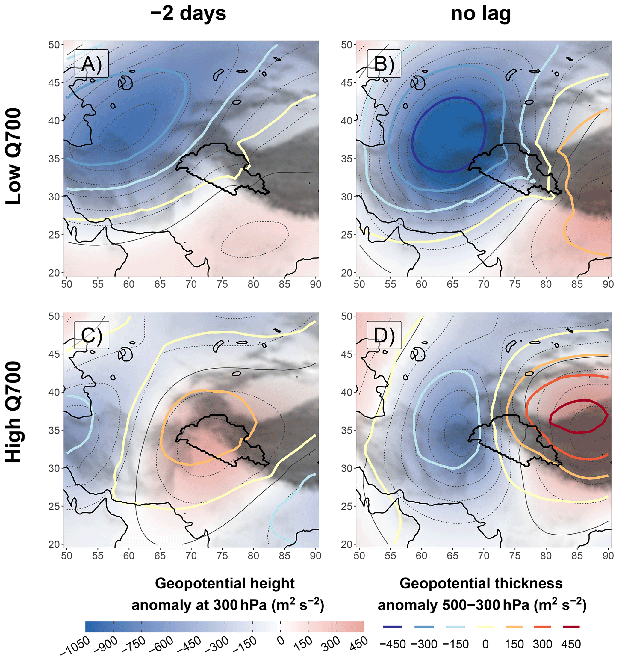
As expected, the two selections exhibit very different patterns of the precipitable water anomaly when UV700 is maximal (Fig. 12e and f). In the case of high Q700, a high positive anomaly is present from the Arabian Sea to north-east India, with a maximum over the UIB, indicating a sustained supply of moisture. By contrast, a negative anomaly is present over the Indus Plain in the case of low Q700, showing that continental dry air is already invading the plain, cutting off any potential moisture supply from the moisture pathway. A small positive anomaly remains in the UIB, probably thanks to the uplifting. Interestingly, no evident difference in the moisture flux direction is visible between the two panels (Fig. 12e and f).
The explanation of the differences in moisture content lies in the circulation history. In the case of high Q700, moisture over the Persian Gulf increases more than in the average case 4 d before the peak of UV700 (Figs. 10b and 12b), due to stronger moisture transport across the Arabian Peninsula. This moisture anomaly moves towards the Indus Plain, the mountain ranges to the west, and even parts of Central Asia 2 d later (Fig. 12d), pushed by a strong southerly component of the moisture flux. The larger extent of the precipitable water anomaly compared to in the average case (Fig. 10c) effectively delays the intrusion of continental dry air (Figs. 12f and 10e). In the low-Q700 case, no such positive anomaly is present (Fig. 12a and c): the WD is not accompanied by a strengthening of the moisture pathway, and the southerly component of the moisture flux is almost absent. Instead, negative anomalies of precipitable water build up over the Tigris–Euphrates plain and Central Asia (Fig. 12c) and move eastwards and south-eastwards, respectively, towards the Indus Plain (Fig. 12c). These patterns show that the balance between moisture advection ahead of a WD and dry air intrusion at the rear may vary significantly.
This difference in the moisture flux can be explained by the origins and tracks of WDs. In the case of high Q700, the mean low at 300 hPa exhibits an eastward motion around 33–34∘ N, which is slightly more to the south than the general case (36∘ N). The WD also exhibits a weaker cold core and a larger zonal gradient of geopotential to its east than in the general case (Figs. 3b and 13d), implying a stronger southerly wind at 700 hPa. Both the southern location and stronger southerly advection at 700 hPa explain how these WDs are able to draw more moisture from the subtropical latitudes along their path. Furthermore, stronger mid-tropospheric warm advection and latent heat release over the mountains to the west of the UIB, due to the higher moisture content, can enhance the wind circulation at 700 hPa so that UV700 remains higher than in the general case (4.4 instead of 4.1 m s−1) despite the weaker geopotential anomaly at 300 hPa (Fig. 13b and d).
By contrast, in the case of low Q700, the mean WD originates from the north-west, towards the Caspian Sea, which means it interacts less with the moisture pathway. The WD is also characterised by a deep cold core, which, despite a stronger geopotential anomaly, results in lower UV700 than in the general case (3.8 m s−1). The WDs are also much slower than in the general case (3.3 m s−1), and, as for the case of lower UV700 discussed in Sect. 4.3.2, we suggest that this is due to the equatorward motion of cold air at the rear of the WD, which is reinforced here by the originally more northern position of the WD. A different way to explain the growing of the WD is through its position relative to the SWJ. The SWJ produces a jet streak to the south-east of the WD. Consequently, such a WD is located on the left entrance of the jet, where convergence and subsidence are enhanced. Therefore, the WD can grow by stretching its vorticity, while the surface cyclonic circulation and the convergence at 700 hPa are reduced. In the meantime, the subsidence leads to a further drying of the atmosphere.
Finally, moisture transport from the trade winds in the Arabian Sea also varies between the two selections: it is stronger (weaker) in the case of lower (higher) Q700, regardless of the position of the WD (arrows, Fig. 12). We discussed with Fig. 10 how trade winds are impacted by the passing of a WD, but trade winds can also impact the moisture field outside of the WD influence. In particular, stronger trade winds transport the moisture evaporating from the Arabian Sea to the Southern Hemisphere, while weaker trade winds allow for a build-up of moisture. Hence, moisture supply to the UIB is also coupled to the tropical and subtropical variability.
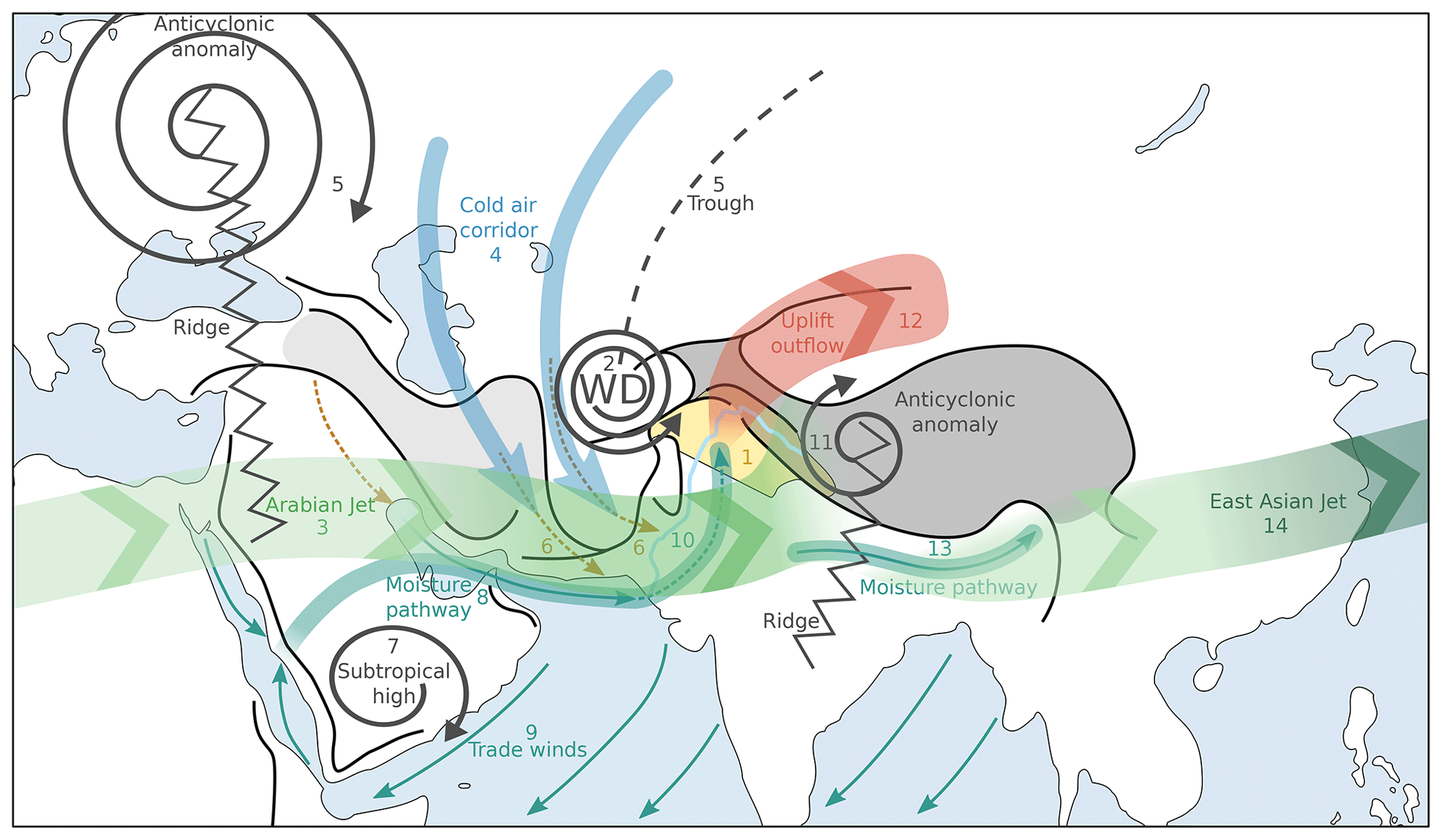
Figure 14Sketch summarising the atmospheric circulation when a WD interacts with the relief to produce precipitation in the UIB. The UIB is in yellow and the Indus River in pale blue. The black lines indicate major mountain ranges and the grey-shaded areas high plateaus (the Tibetan Plateau and the Iranian Plateau). The spirals represent tropospheric geopotential anomalies or centres of actions. The thin sea-green arrows are mean lower-troposphere moisture transport. Thin arrows (e.g. 9 – Trade winds) represent near-surface winds, medium-size arrows (e.g. 4 – Cold air corridor) mid-tropospheric wind, and thick arrows (e.g. 14 – East Asian jet) jets at the tropopause. The dotted brown lines indicate advection of dry air by the WD near the surface. The blue arrows are troposphere-wide cold-air advections. The thick green arrows represent the upper-troposphere jets, with darker colour indicating stronger winds. The red arrow relates to the warm upper-troposphere outflow. Finally, the numbers are in-text references (see Sect. 6).
This study has developed an in-depth analysis of the synoptic variability in precipitation in the Upper Indus Basin (UIB) during winter using PC regressions, quantile regressions, and composites, furthering methods developed in Baudouin et al. (2020a). Several processes explaining the WD growth, decay, interaction with the relief, and relationship with precipitation are suggested. In particular, the atmospheric circulation related to precipitation has been discussed and is summarised in Fig. 14.
Precipitation in the UIB (in yellow, 1) is related to the arrival of an upper-troposphere disturbance from the west (western disturbances, 2). This disturbance is embedded in the subtropical westerly jet, which forms to the west a local maxima, the Arabian jet (3). The upper disturbance grows in part from the equatorward advection of cold air through baroclinic processes (4). This cold air is funnelled between an anticyclonic anomaly and a trough (5) and is responsible for the strengthening the Arabian jet (3). The cold-air advection has an ambivalent role as it is accompanied by dry air close to the surface that can suppress precipitation (6).
Winter moisture transport is driven by the Arabian subtropical high (7). North of it, a westerly moisture pathway (8) connects the Red Sea with the Persian Gulf and the north of the Arabian Sea, while trade winds (9) blow over the rest of the Arabian Sea. The passing of a WD enhances the westerly moisture pathway (8) while it weakens trade winds (9). As the WD approaches the UIB, it steers the moisture across the Indus Plain into the notch formed by the relief (10). The presence of an anticyclonic anomaly east of the WD further enhances the meridional transport (11). This advection of warm and moist air sustains itself, in particular its component close to the surface, through baroclinic and latent heat feedbacks at the synoptic scale.
Eventually, the moisture converges at a low level (around 700 hPa) in the UIB, over the foothills, where the uplift triggers condensation and precipitation (1). It also allows for a mixing and a warming of the air column in the UIB, which counterbalances the cold-air advection associated with the WD (4). In other words, the uplift advects low potential vorticity values to a high altitude (250 hPa) as indicated by the swift anticyclonic turn of its outflow (12), which then increases the zonal gradient of potential vorticity. Consequently, the upper-troposphere cyclonic circulation of the WD further propagates downwards while the baroclinic uplift and the cross-barrier moisture transport increase (10). The increased vertical velocities and high-altitude convergence lead to a break in the Arabian jet (3).
This positive baroclinic interaction, however, is short-lived. Once the WD reaches the UIB, its high-PV anomaly is consumed by the continued advection of low PV, which quickly leads to the weakening of the cyclonic circulation. Furthermore, in addition to this negative baroclinic feedback, dry continental air intrudes into the Indus Plain (6) and cuts off the moisture supply to the UIB, which effectively further suppresses precipitation. The remaining moisture surplus is then pushed towards north-east India (13) while trade winds in the Arabian Sea re-intensify (9). Finally, as the result of the WD interaction with the relief, the subtropical westerly jet weakens to the east of the UIB and this negative anomaly propagates along the East Asian jet in the following days (14).
Winter precipitation and cross-barrier wind in the UIB are unequivocally related to the passing of western disturbances close to the tropopause. However, the idealised scenario presented in Fig. 14 hides large variability in the different features discussed. On the one hand, a PC regression demonstrated that cross-barrier wind is affected not only by how deep the upper geopotential anomaly of the WD is but also by the geopotential gradient east of the WD and by the position and intensity of the cold core of the WD. These characteristics could be used to explain why some WDs trigger very little precipitation. On the other hand, a quantile regression showed that the build-up of moisture in the UIB is dependent on the history of the WD's development and track. The importance of these effects is reinforced by the approximately quadratic relationship that exists between precipitation and cross-barrier moisture transport at 700 hPa and between cross-barrier wind and WD characteristics. The latter may also be related to non-quasi-geostrophic and meso-scale effects, potentially unrelated to WDs (e.g. convection or frontal activity), which have not been explored here but could constitute a topic for future investigations. Other topics whose analyses can build upon the methods and results presented here include the origin of western disturbances and their relation to anticyclonic anomalies over Eastern Europe, the seasonal cycle of precipitation, and its intra-seasonal and inter-annual variability, all of which have been only partially addressed (in e.g. Baudouin, 2020).
The code in R used to produce the figures is available at https://doi.org/10.5281/zenodo.5562173 (Baudouin, 2021).
The ERA-5 data used in this study are freely accessible here: https://doi.org/10.24381/cds.bd0915c6 (Hersbach et al., 2018a).
The original idea, analysis, and text were by JPB with guidance and review from MH and CAP.
The contact author has declared that neither they nor their co-authors have any competing interests.
This paper consists in large part of chap. 4 of the thesis of Jean-Philippe Baudouin, submitted for the degree of Doctor of Philosophy at the University of Cambridge (https://doi.org/10.17863/CAM.68377; Baudouin, 2020).
Publisher's note: Copernicus Publications remains neutral with regard to jurisdictional claims in published maps and institutional affiliations.
We first acknowledge the ECMWF teams in charge of producing the ERA5 reanalysis and sustaining the online availability of the datasets. We also acknowledge our editor and the two reviewers, Ashok Priyadarshan Dimri and Kieran Hunt, for their comments and support to improve the paper.
Jean-Philippe Baudouin thanks the two examiners of his PhD dissertation, Andrew G. Turner and Andrew N. Ross, for their constructive discussions that helped in shaping this paper. Jean-Philippe Baudouin also personally thanks Kira Rehfeld, the STACY group, and the PalMod Phase II project funded by the German Federal Ministry of Education and Research (BMBF), for their support towards the completion of his PhD.
This research was carried out as part of the TwoRains project, which is supported by funding from the European Research Council (ERC) under the European Union's Horizon 2020 research and innovation programme.
This research has been supported by the H2020 European Research Council (grant no. 648609) and BMBF (grant no. 01LP1926C).
This paper was edited by Christian M. Grams and reviewed by Ashok Priyadarshan Dimri and Kieran Hunt.
Agnihotri, C. and Singh, M.: Satellite study of western disturbances, Mausam, 33, 249–254, 1982. a
Ahmed, F., Adnan, S., and Latif, M.: Impact of jet stream and associated mechanisms on winter precipitation in Pakistan, Meteorol. Atmos. Phys., 132, 225–238, https://doi.org/10.1007/s00703-019-00683-8, 2019. a, b, c
Bao, J.-W., Michelson, S. A., Neiman, P. J., Ralph, F. M., and Wilczak, J. M.: Interpretation of Enhanced Integrated Water Vapor Bands Associated with Extratropical Cyclones: Their Formation and Connection to Tropical Moisture, Mon. Weather Rev., 134, 1063–1080, https://doi.org/10.1175/MWR3123.1, 2006. a
Baudouin, J.-P.: A modelling perspective on precipitation in the Indus River Basin: from synoptic to Holocene variability, PhD thesis, University of Cambridge, https://doi.org/10.17863/CAM.68377, 2020. a, b, c, d, e, f, g
Baudouin, J.-P.: Synoptic processes of winter precipitation in the Upper Indus Basin. Weather and Climate Dynamics, Zenodo [code], https://doi.org/10.5281/zenodo.5562173, 2021. a
Baudouin, J.-P., Herzog, M., and Petrie, C. A.: Contribution of Cross-Barrier Moisture Transport to Precipitation in the Upper Indus River Basin, Mon. Weather Rev., 148, 2801–2818, https://doi.org/10.1175/MWR-D-19-0384.1, 2020a. a, b, c, d, e, f, g, h, i, j, k, l, m, n, o, p, q, r, s, t, u
Baudouin, J.-P., Herzog, M., and Petrie, C. A.: Cross-validating precipitation datasets in the Indus River basin, Hydrol. Earth Syst. Sci., 24, 427–450, https://doi.org/10.5194/hess-24-427-2020, 2020b. a, b, c, d
Bollasina, M. and Nigam, S.: Modeling of Regional Hydroclimate Change over the Indian Subcontinent: Impact of the Expanding Thar Desert, J. Climate, 24, 3089–3106, https://doi.org/10.1175/2010JCLI3851.1, 2011. a
Boschi, R. and Lucarini, V.: Water Pathways for the Hindu-Kush-Himalaya and an Analysis of Three Flood Events, Atmosphere, 10, 489, https://doi.org/10.3390/atmos10090489, 2019. a
Brent, R. P.: Algorithms for minimization without derivatives, Prentice-Hall, Englewood Cliffs, New Jersey, 1973. a
Cannon, F., Carvalho, L. M., Jones, C., and Bookhagen, B.: Multi-annual variations in winter westerly disturbance activity affecting the Himalaya, Clim. Dynam., 44, 441–455, https://doi.org/10.1007/s00382-014-2248-8, 2015. a, b
Cannon, F., Carvalho, L. M., Jones, C., and Norris, J.: Winter westerly disturbance dynamics and precipitation in the western Himalaya and Karakoram: a wave-tracking approach, Theor. Appl. Climatol., 125, 27–44, https://doi.org/10.1007/s00704-015-1489-8, 2016. a, b
Chakraborty, A., Behera, S. K., Mujumdar, M., Ohba, R., and Yamagata, T.: Diagnosis of tropospheric moisture over Saudi Arabia and influences of IOD and ENSO, Mon. Weather Rev., 134, 598–617, https://doi.org/10.1175/MWR3085.1, 2006. a
Dacre, H. F., Hawcroft, M. K., Stringer, M. A., and Hodges, K. I.: An Extratropical Cyclone Atlas: A Tool for Illustrating Cyclone Structure and Evolution Characteristics, B. Am. Meteorol. Soc., 93, 1497–1502, https://doi.org/10.1175/BAMS-D-11-00164.1, 2012. a
Dahri, Z. H., Moors, E., Ludwig, F., Ahmad, S., Khan, A., Ali, I., and Kabat, P.: Adjustment of measurement errors to reconcile precipitation distribution in the high-altitude Indus basin, Int. J. Climatol., 38, 3842–3860, 2018. a
Dar, S. S., Ghosh, P., and Hillaire-Marcel, C.: Convection, terrestrial recycling and oceanic moisture regulate the isotopic composition of precipitation at Srinagar, Kashmir, J. Geophys. Res.-Atmos., 126, e2020JD032853, https://doi.org/10.1029/2020JD032853, 2021. a
Datta, R. and Gupta, M.: Synoptic study of the formation and movements of western depressions, Indian J. Meteorol. Geophys, 18, 45–50, 1967. a
de Vries, A. J., Feldstein, S. B., Riemer, M., Tyrlis, E., Sprenger, M., Baumgart, M., Fnais, M., and Lelieveld, J.: Dynamics of tropical–extratropical interactions and extreme precipitation events in Saudi Arabia in autumn, winter and spring, Q. J. Roy. Meteor. Soc., 142, 1862–1880, https://doi.org/10.1002/qj.2781, 2016. a
Dimri, A. and Chevuturi, A.: Model sensitivity analysis study for western disturbances over the Himalayas, Meteorol. Atmos. Phys., 123, 155–180, 2014. a, b, c, d, e
Dimri, A. P.: Impact of horizontal model resolution and orography on the simulation of a western disturbance and its associated precipitation, Meteorol. Appl., 11, 115–127, https://doi.org/10.1017/S1350482704001227, 2004. a
Dimri, A. P.: The transport of momentum, sensible heat, potential energy and moisture over the western Himalayas during the winter season, Theor. Appl. Climatol., 90, 49–63, https://doi.org/10.1007/s00704-006-0274-0, 2007. a, b, c
Dimri, A. P.: Intraseasonal oscillation associated with the Indian winter monsoon, J. Geophys-Res.-Atmos., 118, 1189–1198, https://doi.org/10.1002/jgrd.50144, 2013. a, b
Dimri, A. P. and Niyogi, D.: Regional climate model application at subgrid scale on Indian winter monsoon over the western Himalayas, Int. J. Climatol., 33, 2185–2205, https://doi.org/10.1002/joc.3584, 2013. a, b
Dimri, A. P., Niyogi, D., Barros, A. P., Ridley, J., Mohanty, U. C., Yasunari, T., and Sikka, D. R.: Western Disturbances: A review, Rev. Geophys., 53, 225–246, https://doi.org/10.1002/2014RG000460, 2015. a, b, c, d, e, f, g, h, i, j, k, l
Filippi, L., Palazzi, E., von Hardenberg, J., and Provenzale, A.: Multidecadal variations in the relationship between the NAO and winter precipitation in the Hindu Kush–Karakoram, J. Climate, 27, 7890–7902, 2014. a, b, c, d, e, f, g
Grams, C. M., Wernli, H., Böttcher, M., Čampa, J., Corsmeier, U., Jones, S. C., Keller, J. H., Lenz, C.-J., and Wiegand, L.: The key role of diabatic processes in modifying the upper-tropospheric wave guide: a North Atlantic case-study, Q. J. Roy. Meteor. Soc., 137, 2174–2193, https://doi.org/10.1002/qj.891, 2011. a
Hersbach, H., Bell, B., Berrisford, P., Biavati, G., Horányi, A., Muñoz Sabater, J., Nicolas, J., Peubey, C., Radu, R., Rozum, I., Schepers, D., Simmons, A., Soci, C., Dee, D., and Thépaut, J.-N.: ERA5 hourly data on pressure levels from 1979 to present, Copernicus Climate Change Service (C3S) Climate Data Store (CDS) [data set], https://doi.org/10.24381/cds.bd0915c6, 2018a. a
Hersbach, H., de Rosnay, P., Bell, B., Schepers, D., Simmons, A., Soci, C., Abdalla, S., Alonso-Balmaseda, M., Balsamo, G., Bechtold, P., Berrisford, P., Bidlot, J.-R., de Boisséson, E., Bonavita, M., Browne, P., Buizza, R., Dahlgren, P., Dee, D., Dragani, R., Diamantakis, M.,Flemming, J., Forbes, R., Geer, A., Haiden, T., Hólm, E., Haimberger, L., Hogan, R., Horányi, A., Janiskova, M., Laloyaux, P., Lopez,P., Munoz-Sabater, J., Peubey, C., Radu, R., Richardson, D., Thépaut, J.-N., Vitart, F., Yang, X., Zsótér, E., and Zuo, H.: Operationalglobal reanalysis: progress, future directions and synergies with NWP, ERA-report, Serie 27, https://doi.org/10.21957/tkic6g3wm, 2018b. a
Hewitt, K.: Glacier change, concentration, and elevation effects in the karakoram Himalaya, Upper Indus Basin, Mountain Res. Dev., 31, 188–200, https://doi.org/10.1659/MRD-JOURNAL-D-11-00020.1, 2011. a
Hunt, K. M. and Dimri, A.: Synoptic-scale precursors of landslides in the western Himalaya and Karakoram, Sci. Total Environ., 776, 145895, https://doi.org/10.1016/j.scitotenv.2021.145895, 2021. a
Hunt, K. M., Turner, A. G., and Shaffrey, L. C.: The evolution, seasonality and impacts of western disturbances, Q. J. Roy. Meteor. Soc., 144, 278–290, 2018a. a, b, c, d, e, f, g, h, i, j, k, l, m, n, o, p, q, r
Hunt, K. M., Turner, A. G., and Shaffrey, L. C.: Extreme daily rainfall in Pakistan and north India: scale interactions, mechanisms, and precursors, Mon. Weather Rev., 146, 1005–1022, 2018b. a, b, c, d, e, f, g, h
Hunt, K. M. R., Turner, A. G., and Schiemann, R. K. H.: How interactions between tropical depressions and western disturbances affect heavy precipitation in South Asia, Mon. Weather Rev., https://doi.org/10.1175/MWR-D-20-0373.1, 2021. a, b
Jeelani, G., Deshpande, R. D., Galkowski, M., and Rozanski, K.: Isotopic composition of daily precipitation along the southern foothills of the Himalayas: impact of marine and continental sources of atmospheric moisture, Atmos. Chem. Phys., 18, 8789–8805, https://doi.org/10.5194/acp-18-8789-2018, 2018. a, b
Krishnamurti, T. N.: The subtropical jet stream of winter, J. Meteorol. 18, 172–191, https://doi.org/10.1175/1520-0469(1961)018<0172:TSJSOW>2.0.CO;2, 1961. a, b
Krishnan, R., Sabin, T. P., Madhura, R. K., Vellore, R. K., Mujumdar, M., Sanjay, J., Nayak, S., and Rajeevan, M.: Non-monsoonal precipitation response over the Western Himalayas to climate change, Clim. Dynam., 52, 4091–4109, https://doi.org/10.1007/s00382-018-4357-2, 2018. a
Lang, T. J. and Barros, A. P.: Winter storms in the central Himalayas, J. Meteorol. Soc. Japan. Ser. II, 82, 829–844, 2004. a, b
Madhura, R. K., Krishnan, R., Revadekar, J. V., Mujumdar, M., and Goswami, B. N.: Changes in western disturbances over the Western Himalayas in a warming environment, Clim. Dynam., 44, 1157–1168, https://doi.org/10.1007/s00382-014-2166-9, 2015. a
Mahanta, R., Sarma, D., and Choudhury, A.: Heavy rainfall occurrences in northeast India, Int. J. Climatol., 33, 1456–1469, https://doi.org/10.1002/joc.3526, 2013. a
Malardel, S.: Fondamentaux de météorologie: à l'école du temps, Cépaduès, 2005. a, b, c, d
Malurkar, S. L.: Abnormally dry and wet western disturbances over North India, Curr. Sci., 16, 139–141, 1947. a
Mannan, M. A., Chowdhury, M. A. M., Karmakar, S., Ahmed, S., and Rahman, A.: Analysis and prediction of rainfall associated with Western Disturbances during winter months in Bangladesh, Den-Drop (A Scientific Journal of Meteorology and Geo-physics), Bangladesh Meteorological Department, Dhaka, Bangladesh, 4, 12–24, 2017. a
Martínez-Alvarado, O., Joos, H., Chagnon, J., Boettcher, M., Gray, S. L., Plant, R. S., Methven, J., and Wernli, H.: The dichotomous structure of the warm conveyor belt, Q. J. Roy. Meteor. Soc., 140, 1809–1824, https://doi.org/10.1002/qj.2276, 2014. a
Midhuna, T. M., Kumar, P., and Dimri, A. P.: A new Western Disturbance Index for the Indian winter monsoon, J. Earth Syst. Sci., 129, 59, https://doi.org/10.1007/s12040-019-1324-1, 2020. a, b, c, d, e
Mujumdar, M.: Diagnostic Analysis of Wintertime Rainfall Events Over the Arabian Region, Contribution from IITM, Indian Institute of Tropical Meteorology, ISSN 0252-1075, 2006. a
Mull, S. and Desai, B.: The Origin and Structure of the Winter Depressions of Northwest India, Technical Note 25:18, India Meteorological Department, India, 1947. a
Nathans, L., Oswald, F., and Nimon, K.: Interpreting multiple linear regression: A guidebook of variable importance, Practical Assessment, Research and Evaluation, 17, 1–19, 2012. a
Pisharoty, P. and Desai, B.: Western disturbances and Indian weather, Indian J. Meteorol. Geophys, 7, 333–338, 1956. a
Rakesh, V., Singh, R., Yuliya, D., Pal, P. K., and Joshi, P. C.: Impact of variational assimilation of MODIS thermodynamic profiles in the simulation of western disturbance, Int. J. Remote Sens., 30, 4867–4887, https://doi.org/10.1080/01431160902980332, 2009. a
Rana, S., McGregor, J., and Renwick, J.: Precipitation seasonality over the Indian subcontinent: An evaluation of gauge, reanalyses, and satellite retrievals, J. Hydrometeorol., 16, 631–651, 2015. a
Sankar, N. V. and Babu, C.: Role of vorticity advection and thermal advection in the development of western disturbance during North Indian winter, Meteorol. Atmos. Phys., 132, 515–529, 2020. a
Schiemann, R., Lüthi, D., and Schär, C.: Seasonality and Interannual Variability of the Westerly Jet in the Tibetan Plateau Region, J. Climate, 22, 2940–2957, https://doi.org/10.1175/2008JCLI2625.1, 2009. a, b, c, d
Singh, S. P., Bassignana-Khadka, I., Singh Karky, B., and Sharma, E.: Climate change in the Hindu Kush-Himalayas: the state of current knowledge, Tech. rep., International Centre for Integrated Mountain Development (ICIMOD), Kathmandu, 2011. a
Smith, R. L., Joel W. Ager, J., and Williams, D. L.: Suppressor Variables in Multiple Regression/Correlation, Educ. Psychol. Meas., 52, 17–29, https://doi.org/10.1177/001316449205200102, 1992. a
Syed, F. S., Giorgi, F., Pal, J. S., and Keay, K.: Regional climate model simulation of winter climate over Central–Southwest Asia, with emphasis on NAO and ENSO effects, Int. J. Climato., 30, 220–235, https://doi.org/10.1002/joc.1887, 2010. a, b, c
Thapa, K., Endreny, T. A., and Ferguson, C. R.: Atmospheric Rivers Carry Nonmonsoon Extreme Precipitation Into Nepal, J. Geophys. Res.-Atmos., 123, 5901–5912, https://doi.org/10.1029/2017JD027626, 2018. a
Thomas, L., Dash, S. K., Mohanty, U. C., and Babu, C. A.: Features of western disturbances simulated over north India using different land-use data sets, Meteorol. Appl., 25, 246–253, https://doi.org/10.1002/met.1687, 2018. a
Tinmaker, M. and Ali, K.: Space time variation of lightning activity over northeast India, Meteorol. Z., 21, 135–143, 2012. a
Xueyuan, K. and Yaocun, Z.: Seasonal variation of the East Asian Subtropical Westerly Jet and its association with the heating field over East Asia, Adv. Atmos. Sci., 22, 831–840, https://doi.org/10.1007/bf02918683, 2005. a
Yadav, R. K., Kumar, K. R., and Rajeevan, M.: Characteristic features of winter precipitation and its variability over northwest India, J. Earth Syst. Sci., 121, 611–623, https://doi.org/10.1007/s12040-012-0184-8, 2012. a
Yang, S., Lau, K.-M., Yoo, S.-H., Kinter, J. L., Miyakoda, K., and Ho, C.-H.: Upstream Subtropical Signals Preceding the Asian Summer Monsoon Circulation, J. Climate, 17, 4213–4229, https://doi.org/10.1175/JCLI3192.1, 2004. a
Zhu, Y. and Newell, R. E.: A Proposed Algorithm for Moisture Fluxes from Atmospheric Rivers, Mon. Weather Rev., 126, 725–735, https://doi.org/10.1175/1520-0493(1998)126<0725:APAFMF>2.0.CO;2, 1998. a
This is in contrast to Baudouin et al. (2020a), who used an arbitrary pressure threshold.
This number insures the “extent of pattern” as defined in Baudouin et al. (2020a) is the same; see also Baudouin (2020).
A higher resolution is not needed and would require significantly higher computational power.
This is the usual quantile and is not based on a quantile regression.
- Abstract
- Introduction
- Season, data, and study area
- Methods
- Results regarding the wind contribution
- Relating moisture contribution variability to western disturbances
- Summary
- Code availability
- Data availability
- Author contributions
- Competing interests
- Disclaimer
- Acknowledgements
- Financial support
- Review statement
- References