Impact of Eurasian autumn snow on the winter North Atlantic Oscillation in seasonal forecasts of the 20th century

As the leading climate mode of wintertime climate variability over Europe, the North Atlantic Oscillation (NAO) has been extensively studied over the last decades. Recently, studies highlighted the state of the Eurasian cryosphere as a possible predictor for the wintertime NAO. However, missing correlation between snow cover and wintertime NAO in climate model experiments and strong non-stationarity of this link in reanalysis data are questioning the causality of this relationship.

Here we use the large ensemble of Atmospheric Seasonal Forecasts of the 20th Century (ASF-20C) with the European Centre for Medium-Range Weather Forecasts model, focusing on the winter season. Besides the main 110-year ensemble of 51 members, we investigate a second, perturbed ensemble of 21 members where initial (November) land conditions over the Northern Hemisphere are swapped from neighboring years. The Eurasian snow–NAO linkage is examined in terms of a longitudinal snow depth dipole across Eurasia. Subsampling the perturbed forecast ensemble and contrasting members with high and low initial snow dipole conditions, we found that their composite difference indicates more negative NAO states in the following winter (DJF) after positive west-to-east snow depth gradients at the beginning of November. Surface and atmospheric forecast anomalies through the troposphere and stratosphere associated with the anomalous positive snow dipole consist of colder early winter surface temperatures over eastern Eurasia, an enhanced Ural ridge and increased vertical energy fluxes into the stratosphere, with a subsequent negative NAO-like signature in the troposphere. We thus confirm the existence of a causal connection between autumn snow patterns and subsequent winter circulation in the ASF-20C forecasting system.

1 Introduction

As the leading climate variability pattern affecting winter climate over Europe, the North Atlantic Oscillation (NAO) has been extensively studied over the last decades (Wanner et al., 2001; Hurrell and Deser, 2010; Moore and Renfrew, 2012; Deser et al., 2017). The NAO state strongly impacts the hydroclimate as well as the ecological and socioeconomic conditions over major population clusters of Europe and North America. In its positive state, the NAO projects onto strong pressure gradients over the North Atlantic, strong westerly winds and mild but wet conditions for central Europe. A negative winter NAO is connected to a southwardly displaced Atlantic jet stream, weaker westerlies, and cold, dry conditions for central Europe. The NAO also shows a distinct quadrupole signature in surface temperature straddling the Atlantic, with two opposite poles over northern Europe and Greenland/Labrador and an opposite pair further south over southern Europe/northern Africa and the US East Coast. Recent cases of extreme negative NAO states (Lü et al., 2020), including the winter 2020/2021, coincided with several extreme weather events across the Northern Hemisphere, including cold air outbreaks with record snowfall at locations over southern and northern Europe, as well as eastern parts of Canada and the United States (Blunden and Boyer, 2021).

Improving seasonal to decadal predictions of the winter NAO is thus a high-priority research for many weather and climate-related research centers (Kang et al., 2014; Scaife et al., 2014, 2016; Smith et al., 2016; Dunstone et al., 2016; Athanasiadis et al., 2017; Weisheimer et al., 2017, 2019; Baker et al., 2018). Despite its stochastic behavior, the NAO state was shown to be modulated by slowly varying components of the climate system, carrying the climate state memory across months or even seasons (Dobrynin et al., 2018; Meehl et al., 2021). Initially discussed by Cohen and Enthekhabi (1999), recent studies have highlighted the potential of Eurasian autumn snow cover anomalies as a useful predictor for the boreal wintertime (December–January–February, DJF) NAO in empirical prediction models (Cohen et al., 2007, 2014; Cohen and Jones, 2011; Peings et al., 2013; Tian and Fan, 2015; Wang et al., 2017; Han and Sun, 2018; Wegmann et al., 2020).

The causal chain behind the snow impact is hypothesized as follows: due to the radiative and thermodynamical properties of snow (Cohen and Rind, 1991; Vavrus, 2007; Dutra et al., 2011; Thackeray et al., 2019), a thicker snowpack is associated with coherent surface cooling. Cohen et al. (2007; see also Cohen et al., 2014; Henderson et al., 2018, for reviews) proposed a multi-step mechanism whereby this surface cooling leads to raised isentropic surfaces, triggering increased Rossby wave activity propagating upward and being absorbed in the stratosphere, warming it and subsequently weakening the polar vortex. The negative stratospheric Northern Annular Mode signal eventually propagates down into the troposphere and to the surface where it projects onto a negative NAO.

Investigating the robustness of this mechanism is challenged by several elements. Observational studies analyzing statistical links are restricted by the relatively short length (a few decades) of comprehensive and complete snow cover observations. Using long-term reanalyses, recent studies showed substantial non-stationary relationships between autumn Eurasian snow cover and the sign of the winter NAO over the span of the 20th century (Peings et al., 2013; Douville et al., 2017; Wegmann et al., 2020). Using shorter time scales, the probability of cherry-picking a period of positive correlation and sampling co-variability with other climate system components increases considerably. Causes for the non-stationarity are still discussed, with possible influences from the Quasi-Biennial Oscillation (QBO), El Niño–Southern Oscillation (ENSO) or simply snow cover variance (Peings et al., 2017; O'Reilly et al., 2017; Tyrrell et al., 2018; Wegmann et al., 2020; Weisheimer et al., 2020). Disentangling co-variability is further challenged by the co-occurrence of increased Eurasian snow cover and increased Ural blocking frequency, questioning the lead–lag relationship between snow cover and blocking (Peings, 2019; Kretschmer et al., 2018; Song and Wu, 2019; Santolaria-Otín et al., 2021). Moreover, a variety of temporal and spatial snow cover indices used among the different studies obstruct direct comparisons. Nevertheless, recent studies point out that a November longitudinal snow cover dipole across Eurasia shows the strongest statistical link to the DJF NAO state (Gastineau et al., 2017; Han and Sun, 2018; Santolaria-Otín et al., 2021).

Analyzing the snow → NAO mechanism in modeling experiments is challenged by shortcomings of the current atmospheric or atmosphere–ocean general circulation models (AGCMs or AOGCMs) regarding snow–atmosphere feedbacks (Santolaria-Otín and Zolina, 2020). Most of the free-running Coupled Model Intercomparison Project (CMIP) models do not capture the statistical snow–NAO link found in reanalyses data (Hardimann et al., 2008; Furtado et al., 2015; Gastineau et al., 2017). On the other hand, when large snowpack anomalies are prescribed through nudging or imposed as initial conditions, several AGCM experiments showed promising results for identifying several to all steps of the proposed mechanism (Gong et al., 2003; Fletcher et al., 2009; Peings et al., 2012; Tyrrell et al., 2018).

Some of the current-generation subseasonal-to-seasonal or seasonal coupled prediction models also seem to catch parts of the mechanism chain, specifically negative temperature anomalies associated with a thicker snowpack (Orsolini et al., 2013; Diro and Lin, 2020) as well as an enhanced wave activity generating upward fluxes into the stratosphere associated with ridging over Eurasia (Orsolini et al., 2016; Li et al., 2019; Garfinkel et al., 2020), although several models failed to simulate that ridging in Garfinkel et al. (2020). The subsequent stratosphere–troposphere coupling influencing the surface Arctic Oscillation also tended to be weak to non-existent in most models. These studies have been limited to the recent decades, and, consequently, confidence in the robustness of the mechanism across spans of decades is still low (Garfinkel et al., 2020).

To disentangle the issues of non-stationarity (found in observations) and causality (found in models), we base our investigation on a 110-year-long (1901–2010) ensemble seasonal prediction experiment, which consists of the historical seasonal hindcasts using ECMWF's atmosphere-only model, called “ASF-20C” (Weisheimer et al., 2017). This 51-member ensemble of hindcasts with four start dates per year and a length of 4 months has been used in several studies on the predictability of the NAO and other climate patterns (e.g., O'Reilly et al., 2017; Parker et al., 2019; Weisheimer et al., 2019, 2020; O'Reilly et al., 2020). To investigate the influence of land surface conditions, in this case snow cover, on the evolution of the atmospheric state throughout the season, we use a novel, 21-member twin set of the ASF-20C forecasts with perturbed initial land conditions. This dataset was used as a pilot experiment in the context of the Land Surface, Snow and Soil moisture Model Intercomparison Program LS3MIP (Van den Hurk et al., 2016), aimed at reproducing land surface potential predictability experiments as described by Dirmeyer et al. (2013). We aim to address the question of causality, pathway, stationarity and seasonal evolution of the proposed mechanism of the snow–stratosphere–troposphere linkage over decadal to centennial time scales.

This paper is organized as follows. Section 2 describes the data and methods used. In Sect. 3, we show winter evolution of climate anomalies for the different initialization runs and contrast them with observed anomalies. The results are discussed in Sect. 4 and finally summarized in Sect. 5.

2 Data and methods

2.1 Climate reanalysis and reconstruction

We use the European Centre for Medium-Range Weather Forecasts (ECMWF) product ERA-20C (ERA20C; Poli et al., 2016) to investigate pre-conditions and the initialization of the seasonal predictions, to compute the DJF NAO index, and to create a Eurasian snow dipole index. ERA-20C only assimilates surface pressure and marine wind observations, with sea surface temperature (SST) boundary conditions taken from the HadISST2.1.0.0 datasets (Rayner et al., 2003). ERA-20C was found to represent interannual snow variations over Eurasia remarkably well. For an in-depth discussion of its performance and the technical details concerning snow computation, see Wegmann et al. (2017b). Due to the aforementioned statistical impact for the winter NAO evolution, we focus on the November Eurasian snow dipole index as a predictor for the following NAO state (Gastineau et al., 2017; Han and Sun, 2018; Santolaria-Otín et al., 2021). Following Han and Sun (2018), who explicitly selected western and eastern domains because of the high co-variance with DJF NAO, we calculate the index over the period 1901–2010 by averaging snow depths over the western domain (48–58^∘ N, 30–60^∘ E) and the eastern domain (40–56^∘ N, 80–130^∘ E), eventually subtracting the western domain from the eastern domain to derive the west–east snow depth gradient. Hence, a positive snow index indicates higher snow depths in the eastern domain and a positive longitudinal snow depth gradient. The index is normalized and linearly detrended with respect to the overall period. To comply with the initialization date of 1 November for the seasonal hindcasts, we calculate the index for 1 November instead of November mean snow (Fig. 1a). Even though Han and Sun (2018) calculated the dipole index using snow cover, we used snow depth since ERA-20C provides snow depth as the actual prognostic variable. We hence refrained from using empirical rules to convert snow depth to snow cover. We found the index based on snow depth to be virtually identical (also see Fig. S1 in the Supplement) to the index using snow cover (see also Wegmann et al., 2020, for more insights).

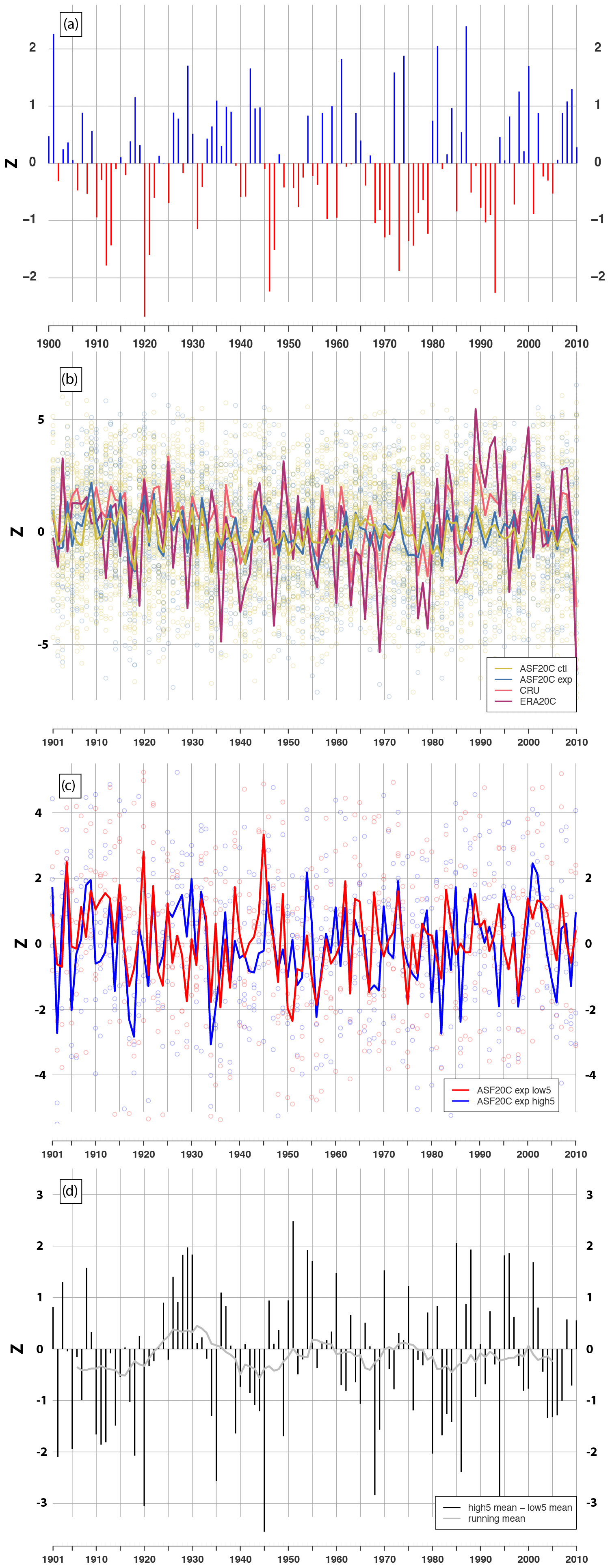
Figure 1 (a) Normalized 1 November Eurasian snow dipole index for the period 1900–2010 as derived from ERA20C. (b) Normalized DJF NAO index in the CRU station-based reconstruction, ERA20C EOF-based index, ASF-20C CTL and ASF-20C EXP EOF-based index. Hollow points represent individual members; solid lines represent ensemble means or observational products. (c) Five-member DJF NAO forecasts for the high- and low-dipole members within ASF-20C EXP. Hollow points represent individual members; solid lines represent ensemble means. (d) NAO DJF state difference and its 11-year running mean between the ASF-20C EXP high- and low-dipole ensemble mean in panel (b) (51 (18) cases of positive (+1 SD) NAO response; 59 (29) cases of negative (−1 SD) NAO response). For 2 SD exceedance, the number of cases is 2 vs. 9.

To compute the winter NAO index, we normalize the first empirical orthogonal function of ERA-20C DJF sea level pressure (SLP) for the region (20–80^∘ N, 90–50^∘ E). We use the same approach to calculate the NAO DJF index based on the seasonal hindcasts and compare those with the reconstructed, independent DJF NAO index by Jones et al. (1997) from the Climate Research Unit (CRU).

2.2 Seasonal prediction experiments

Additionally, we use atmospheric seasonal retrospective hindcasts covering the 110-year period 1901–2010 of ERA-20C with 51 ensemble members of the ASF-20C hindcasts (hereafter ASF-20C CTL) (Weisheimer et al., 2017). The atmospheric model used for the 4-month hindcasts is the ECMWF Integrated Forecast System version CY41R1 and is initialized at four start dates per year (1 February, May, August and November) with ERA20C land and atmospheric conditions. It uses the same lower-boundary conditions for SST and sea ice as ERA-20C. Here, we only use hindcasts initialized on 1 November. The horizontal spectral resolution of the model of T255 is similar to ECMWF's previous operational system System 4 (Molteni et al., 2011) and corresponds to a grid length of approximately 80 km. The model has 91 vertical levels and a top at 0.01 hPa. The ensemble has been created by perturbing each member through the stochastic physics schemes to represent model uncertainties in a similar way as the aforementioned System 4.

To investigate the impact of Eurasian snow depth we use an additional set of perturbed hindcasts, based on a 21-member subset of the ASF-20C CTL experiment (hereafter, the “experiment” or ASF-20C EXP). Each member run is initialized with different land surface conditions, sampled from the neighboring 20 years. For example, the range of land surface conditions for the 21-member ensemble forecast initialized on 1 November 1950 spans the land surface conditions of the years 1940–1960: member 01 is initialized with the land surface conditions of 1940, member 02 with conditions of 1941, member 03 with conditions of 1942 and so forth. For the beginning and ending 10 years of the hindcast dataset, the land surface conditions are sampled from the closest 21 neighboring years within the dataset. Here, land surface conditions include the entire land state, including soil moisture, snow depth and soil temperatures. We argue that for investigating Northern Hemisphere climate anomalies of the 1 November initialization, snow depth has by far the largest impact on atmospheric dynamics compared to soil moisture and soil temperatures, thus allowing us to attribute the differences to snow changes. The main bulk of the experiment data have a monthly resolution, and daily data are only available for selected variables and three tropospheric levels. After initialization, oceanic components like SSTs and sea ice are prescribed and based on observations among all members in ASF-20C CTL and ASF-20C EXP.

Taking advantage of the shuffled initial land conditions of ensemble members in ASF-20C EXP, we subsample members with positive or negative initial Eurasian snow dipole (Fig. 2). This conditional sampling approach has been used when testing the sensitivity of extended range forecasts to soil moisture (Koster et al., 2011; van den Hurk et al., 2012) or to snow initial conditions (Li et al., 2019; Garfinkel et al., 2020). For each start date, we can identify those members with positive or negative initial snow dipole indices, corresponding to different years of the shuffled land initialization. We further proceed with compositing these two selected sets. Due to the decadal variability in the November snow cover, the amount of “high snow dipole members” (positive dipole index) and “low snow dipole members” (negative dipole index) varies throughout the 110 years. There might be periods when a majority of the neighboring 20 years shows a positive snow dipole index and other periods when a minority does. To avoid this variation of the composited ensemble size across the years, we only use the five ensemble members with the most positive and most negative initial Eurasian snow dipole, creating two ensemble means (each of size N=5), namely a high snow dipole ensemble mean and low snow dipole ensemble mean, for each winter through the 110-year period.

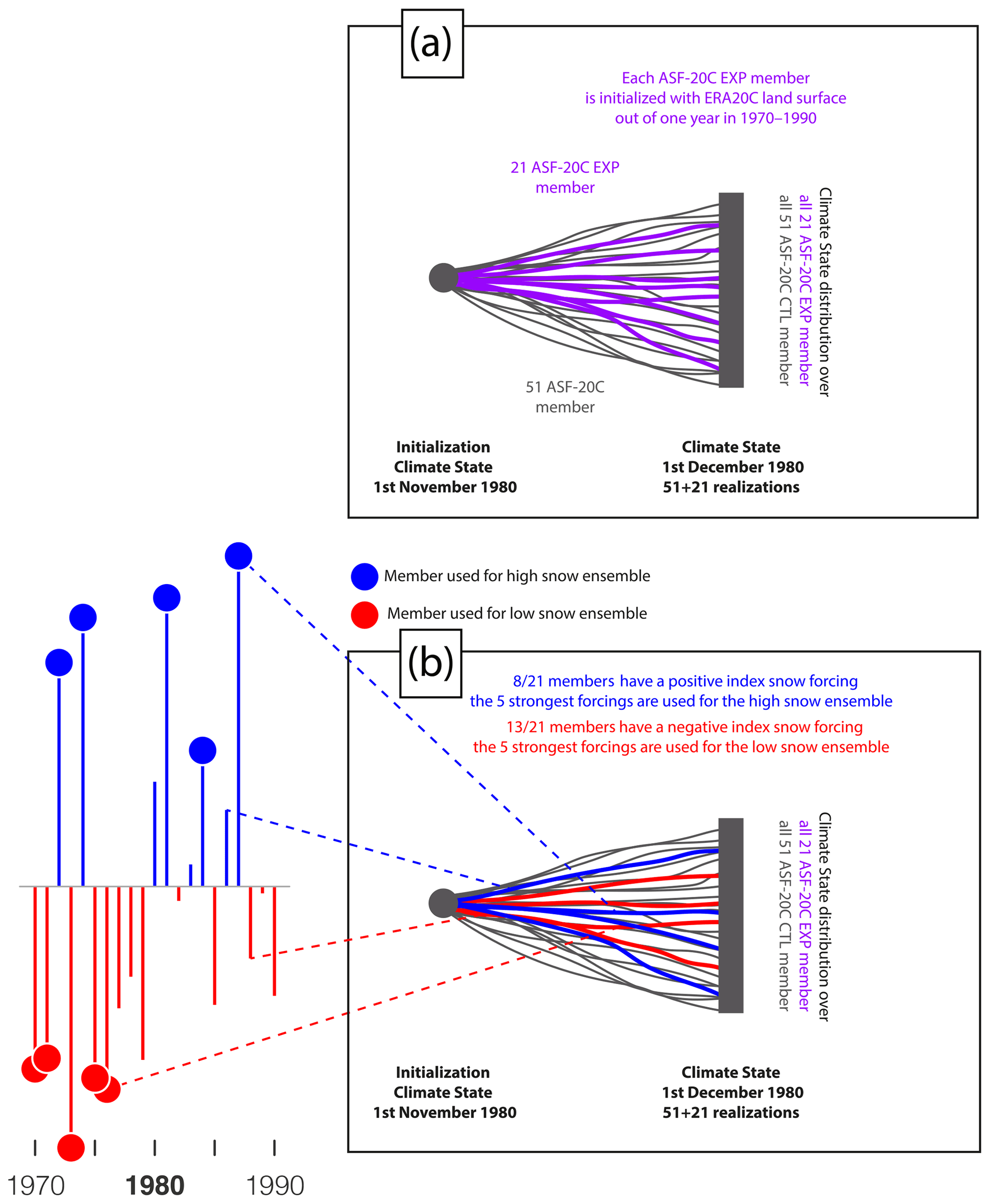
Figure 2 As an example, the schematic for (a) the 1 November 1980 ASF-20C EXP initialization and the consequent sampling of the 21 ensemble members into the high and low snow dipole ensembles. For the 1 November initialization, ASF-20C EXP members are initialized by land surface conditions of the 21 surrounding 1 November dates, in this case 1970–1990. (b) Out of these 21 members, we sample individual members based on their ranking in the snow index. The five members with the most positive snow index constitute the high snow ensemble and vice versa for the low snow ensemble.

It should be noted that the absolute magnitude of the ensemble mean snow differences is still changing from year to year. For example, the most positive snow dipole for the period 1910–1930 might be lower than in the time window 1980–2000, and the same applies for negative dipole indices. Due to the definition of the ASF-20C EXP, this setup is unavoidable, but it also allows for realistic magnitudes of snow forcings and for incorporating a realistic natural variability into the experiment. The (five-member) ensemble mean difference (Fig. 3a) displays a snow depth increase of 1–2 cm over central and eastern Siberia, together with a 0.2–1 cm snow depth decrease over western Russia, as expected from the snow dipole definition. Concomitant negative anomalies (1–2 cm snow depth) nevertheless extend outside of the dipole definition domains to more northern latitudes, e.g., over western Russia and the Russian Far East, or over the coastal mountain ranges of the North American Pacific Northwest. Note that the two domains forming the dipole are in snow transition zones, where the snow cover is rare on 1 November (Fig. 3b, c). The dipole positive phase corresponds to anomalously high snow depths over eastern Eurasia, where the ERA20C snow depth climatology indicates a few centimeters of snow. It also corresponds to anomalously low snow over the west of Russia, in regions with no to rare snow cover in the ERA20C 1 November climatology. The eastern domain partly covers the Mongolian Plateau region, which was shown to exert a strong impact of the wintertime wave fluxes in the stratosphere (White et al., 2017).

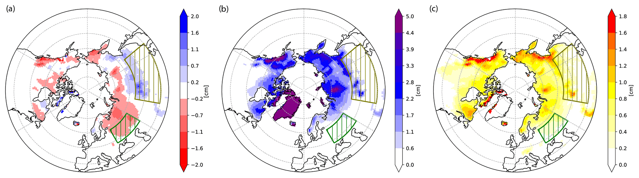
Figure 3 (a) Average (1900–2010) 1 November snow depth difference between the high-dipole and low-dipole ensemble. (b) Average (1900–2010) 1 November snow depth. (c) Average (1900–2010) 1 November snow depth standard deviation. Hatched in green (olive) is the western (eastern) domain of the snow index. All three plots are based on ERA20C.

If not stated otherwise we compute differences between the five-member ensemble means of the high snow dipole and low snow dipole in ASF-20C-EXP as well as differences of each ensemble mean relative to the ensemble mean of ASF-20C CTL. We compute significance using a two-sided Student t test.

3 Results

3.1 DJF NAO comparison

Figure 1b shows the time series of the normalized reconstructed (i.e., based on station data), reanalyzed and predicted winter NAO state for the period 1901–2010. Unsurprisingly, the ensemble means of the ASF-20C CTL and ASF-20C EXP hindcasts show reduced temporal variance compared to the observation-based NAO datasets. However, single realizations and member spread of the CTL and EXP runs cover the whole range of variability displayed by the observation-based product (see also Fig. S2).

The correlation between the ERA-20C and CRU NAO index is 0.83, indicating that the EOF approach is a good approximation of the station-based index. It should be noted that the DJF average has a higher correlation between hindcasts and reanalyses than the individual months within the season (see Table S1).

The ASF-20C CTL ensemble mean DJF hindcasts achieve an overall correlation of 0.33 with the CRU NAO reconstruction for the complete time period, with ASF-20C EXP having a nearly identical correlation (0.34). This near-identical correlation is expected given that the land state perturbations across the 21 members are two sided. Differences between the predicted NAO index of ASF-20C CTL and EXP ensemble means are generally small, with the NAO indices having the same sign during most winters. The correlation between CTL and EXP is 0.8 for the 110-year period. The slightly stronger variability of ASF-20C EXP can partly be attributed to the reduced ensemble size.

Contrasting the (initial) high-dipole and low-dipole composites constructed from the ASF-20C EXP ensemble, we see decadal variability in the difference of winter-mean NAO (Fig. 1c, d). The first two decades of the 20th century are characterized by rather strong negative NAO responses to a strong positive snow dipole. This is followed by two decades spanning the early 20th century Arctic warming (Polyakov et al., 2003), which shows the opposite response: a strongly positive west–east snow depth gradient, as depicted in Fig. 3, leads to more positive NAO-like states compared to a weak west–east snow depth gradient. After several decades with changing responses to the snow anomaly between the two ensembles, eventually the 21st century starts with a weak negative NAO response to a strong positive snow dipole. Averaged over the whole period, the high snow dipole ensemble shows a slightly stronger negative NAO response: 51 cases of positive NAO response versus 59 cases of negative NAO response. For more extreme NAO states (1 SD exceedance), the difference is more pronounced, 18 versus 29, and for 2 SD exceedance, the difference is 2 versus 9. Possible reasons for the decadal response to the snow forcing will be considered in the discussion section.

3.2 Regression analysis

Previous studies showed that regressing observed boreal winter zonal-mean temperature and zonal wind anomalies onto an observed Eurasian autumn snow index reveals a significant stratospheric warming and slowdown of the polar vortex starting in November, migrating down towards the tropopause until February (Wegmann et al., 2020). A similar relation between Eurasian snow and the polar stratosphere can be found in the dataset used here.

Figure 4 shows a strongly reduced polar vortex for the ERA20C autumn to winter climate anomalies regressed on the November snow dipole index. The zonal wind anomalies in the troposphere highlight a weakened polar jet and an increased subtropical jet, especially in January and February. The concurrent polar stratospheric warming signal moves towards the upper troposphere throughout the winter months, with peak warming at around 100 hPa in February.

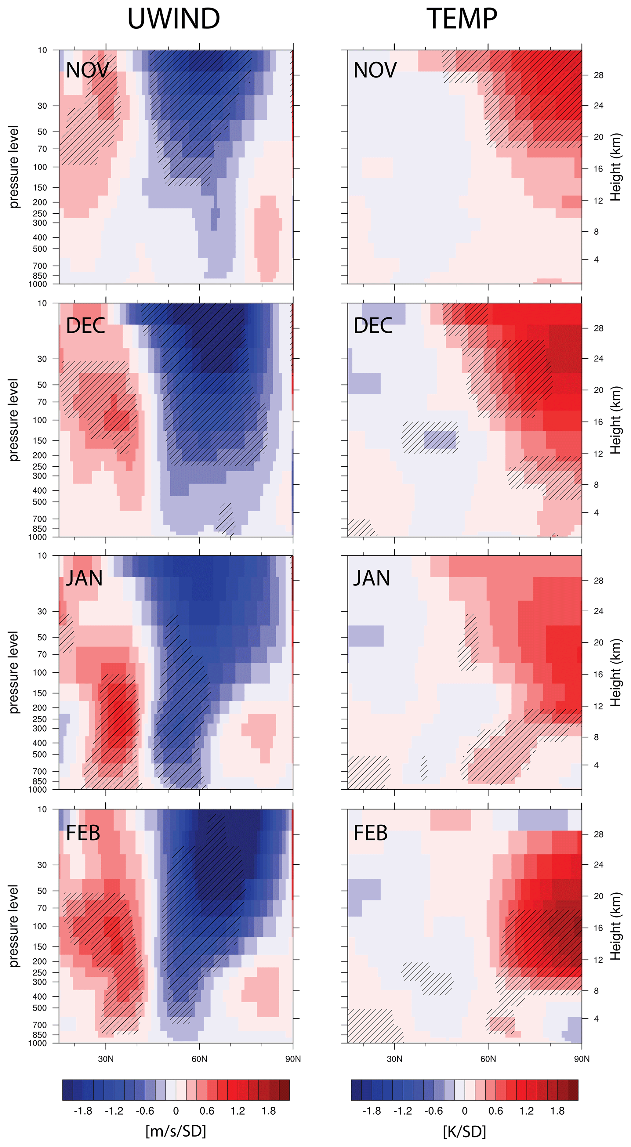
Figure 4 Zonal-mean meridional cross section of ERA20C anomalies in temperature and zonal wind regressed onto the snow dipole index in November from ERA20C covering 1901–2010 for November, December, January and February. Shading indicates 95 % significance level.

Spatially, pressure anomalies regressed onto the November snow dipole index reveal that the geographical center of the stratospheric warming is located over the Canadian Arctic (Fig. 5). Tropospheric pressure differences highlight a strong ridging over western Russia and the Ural Mountains in December, which subsequently over the course of winter is shifted more towards Greenland and the northern North Atlantic region, reflecting a negative NAO-like atmospheric state. This state is further supported by negative DJF SLP anomalies over southern Europe and the Mediterranean region. Downstream of the Eurasian snow signal, a negative SLP anomaly is found over the northern North Pacific. The question remains of whether these patterns derived by the regression analysis are a result of co-variability, common climate drivers or causal physical processes.

Figure 5 ERA20C anomalies of 10 hPa (a, b) geopotential heights, (c, d) 500 hPa geopotential heights and (e, f) sea level pressure regressed onto the snow dipole index in November from ERA20C covering 1901–2010 for December and DJF mean. Shading indicates 95 % significance level. For monthly anomalies see Fig. S9.

3.3 Spatial anomalies in the experiment

In the following, we investigate the spatial differences in the atmospheric response associated with the high and low snow dipole ensemble means of ASF-20C EXP, focusing on the initial response in December as well as the average DJF response, as the November response is not yet significant for almost all climate variables.

Figure 6a and b show stratospheric geopotential heights anomalies at 10 hPa. In December, a significant negative anomaly formed above Eurasia, corresponding to a polar vortex displacement toward the Eurasian sector and a high over Alaska (albeit not significant), as commonly found during stratospheric warming events. Over the course of the winter, this pattern develops into increased geopotential heights over the Arctic with significantly reduced geopotential heights over the extratropics, albeit only significant over southern Europe and the Caucasus.

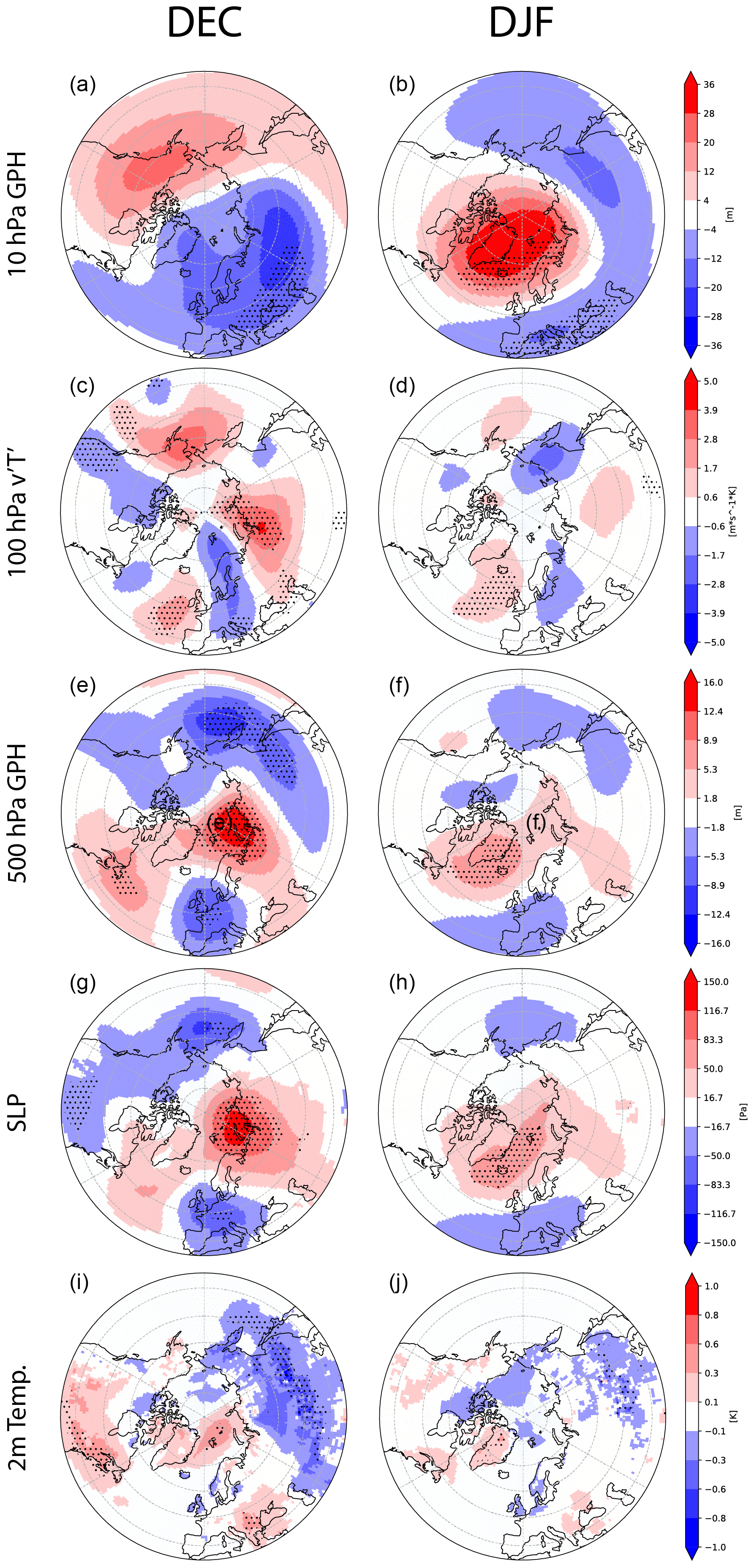
Figure 6 Averaged anomalies in 1901–2010 between high-dipole and low-dipole ASF-20C EXP ensemble means for December (a, c, e, g, i) and DJF (b, d, f, h, j): (a, b) 10 hPa geopotential heights, (c, d) 100 hPa meridional eddy heat flux, (e, f) 500 hPa geopotential heights, (g, h) sea level pressure and (i, j) 2 m temperature. Stippled areas represent 90 % significance. For monthly anomalies see Fig. S10.

To better understand the wave activity flux into the stratosphere, we investigated the meridional eddy heat flux at 100 hPa, which is proportional to the vertical component of the wave activity flux (Fig. 6c): it highlights a wave train of circumpolar anomalies in December (hence following the surface signal forcing in November) with significant positive anomalies over the Ural Mountains, eastern North Pacific, and the European part of the North Atlantic and negative anomalies over central and northern Europe and along the North American Pacific coast. The average DJF response highlights a circumpolar wave train but shows significant anomalies only for the increased northward heat flux over the northern North Atlantic.

Tropospheric circulation anomalies are depicted for geopotential heights at 500 hPa in Fig. 6e and f. In December, a strong positive anomaly is located over the Barents–Kara Sea sector, with significantly negative anomalies upstream and downstream. A second region of positive anomalies emerges at the Canadian Atlantic coast. Both regions match the significant positive anomalies in the 100 hPa heat flux well. The averaged DJF anomalies highlight a negative mid-tropospheric NAO signal with significantly increased geopotential heights above Greenland and Iceland.

Sea level pressure anomalies largely mirror the 500 hPa geopotential height anomalies. The averaged DJF pattern only shows significant positive anomalies over the northern North Atlantic but still projects onto a meridional pressure gradient characteristic of a negative NAO anomaly (Fig. 6h). It is important to note that the absolute difference is rather small compared to interannual SLP variability. Anomalies between the two ensemble means are less than 1 hPa. Even though this number can be assumed to be smaller than in observational datasets due to the ensemble averaging process, it only constitutes about 15 % of the average 1901–2010 DJF SLP standard deviation over the Euro-Atlantic sector.

Due to its large variability, composites of the near-surface temperature are largely non-significant (Fig. 6i, j). Yet, in December a clear cooling signal emerges over central and eastern Eurasia, as expected from the location of the positive snow anomalies at the time of forecast initialization. At the same time, eastern North America and southeastern Europe show significant positive temperature anomalies, a result of northward heat advection at the eastern flanks of low-pressure anomalies (Fig. 6g). Averaged DJF 2 m temperatures are significant only for Greenland and eastern Eurasia, with the cooling over the latter a direct result of the persistence of the anomalously high initial snowpack.

3.4 Vertical anomalies in the experiment

To get a better understanding on how the different land initial conditions impact the vertical distribution of temperature and zonal wind, Fig. 7 shows meridional cross sections of the zonal-mean anomalies of zonal wind and temperatures from November to February.

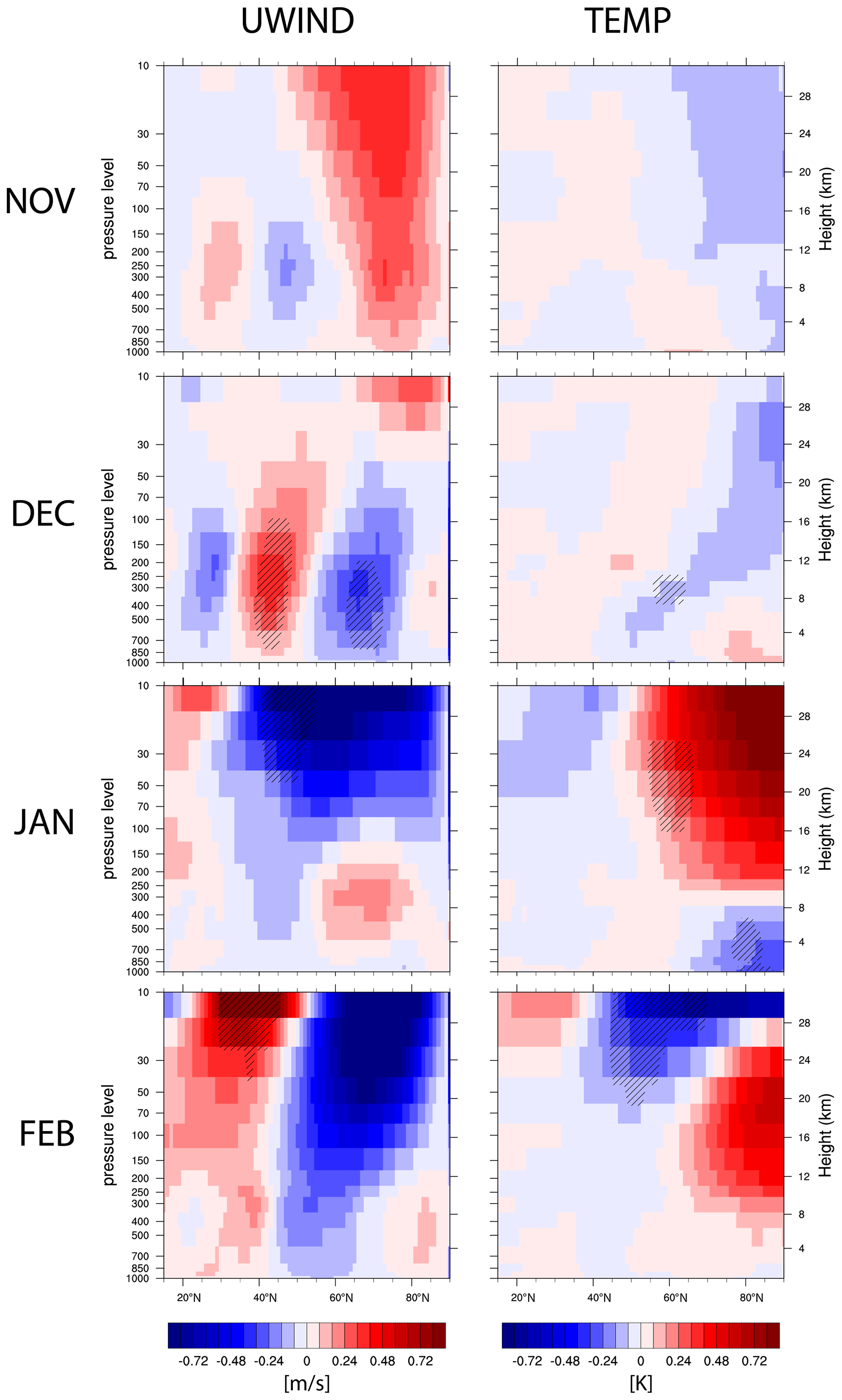
Figure 7 Zonal-mean cross section of (left) zonal wind anomalies and (right) temperature anomalies for the period 1901–2010 between high-dipole and low-dipole ASF-20C EXP ensemble means. Shading indicates 90 % significance level.

While November anomalies (Fig. 7) are overall insignificant, a strong snow dipole is associated with an increased polar vortex and cooler stratosphere. In December, zonal wind anomalies are indicative of the tropospheric subtropical jet shifted northward concurrent with a weak Arctic surface warming. Changes are substantial in January, when the stratospheric polar vortex is significantly weakened, with a slight increase in westerlies in the mid-troposphere. The corresponding temperature anomalies show a widespread stratospheric warming and negative anomalies in the lower Arctic troposphere. Eventually in February, the slowdown of westerlies is predicted to reach all the way down from the stratosphere into the troposphere. On the southern flank of these negative zonal wind anomalies, westerly winds are increasing, especially so in the stratosphere. The stratospheric warming signal migrates downwards to the lower stratosphere and tropopause layer. As the warming has migrated down, a stratospheric cooling is occurring aloft.

As a further confirmation, polar cap heights (Fig. S3) reveal a development of positive anomalies from the surface in December up to the stratosphere in January, migrating back to the troposphere in February. Note that the development of these anomalies is delayed compared to the one shown in the ERA20-C reanalyses (compare Figs. 4 and 7) since initial atmospheric conditions are identical in the perturbed ensemble members.

3.5 Daily evolution of anomalies in the experiment

To investigate the temporal evolution of important tropospheric anomalies, Fig. 8 shows daily mean 500 hPa geopotential height anomalies (high minus low snow dipole ensembles) averaged over 60–70^∘ N. The Hovmøller diagram illustrates the Ural ridge developing only at the end of November going into December and preceding the development of the North Atlantic ridge, which is the main component of the negative NAO-like feature in our results. It should also be noted that the absence of meaningful anomalies during the first 10 d of the composite difference again reflects the identical tropospheric anomalies arising from the pre-conditions. The anomalies generated by the end of November do indeed arise from the impact of snow cover differences and snow–atmosphere feedbacks.

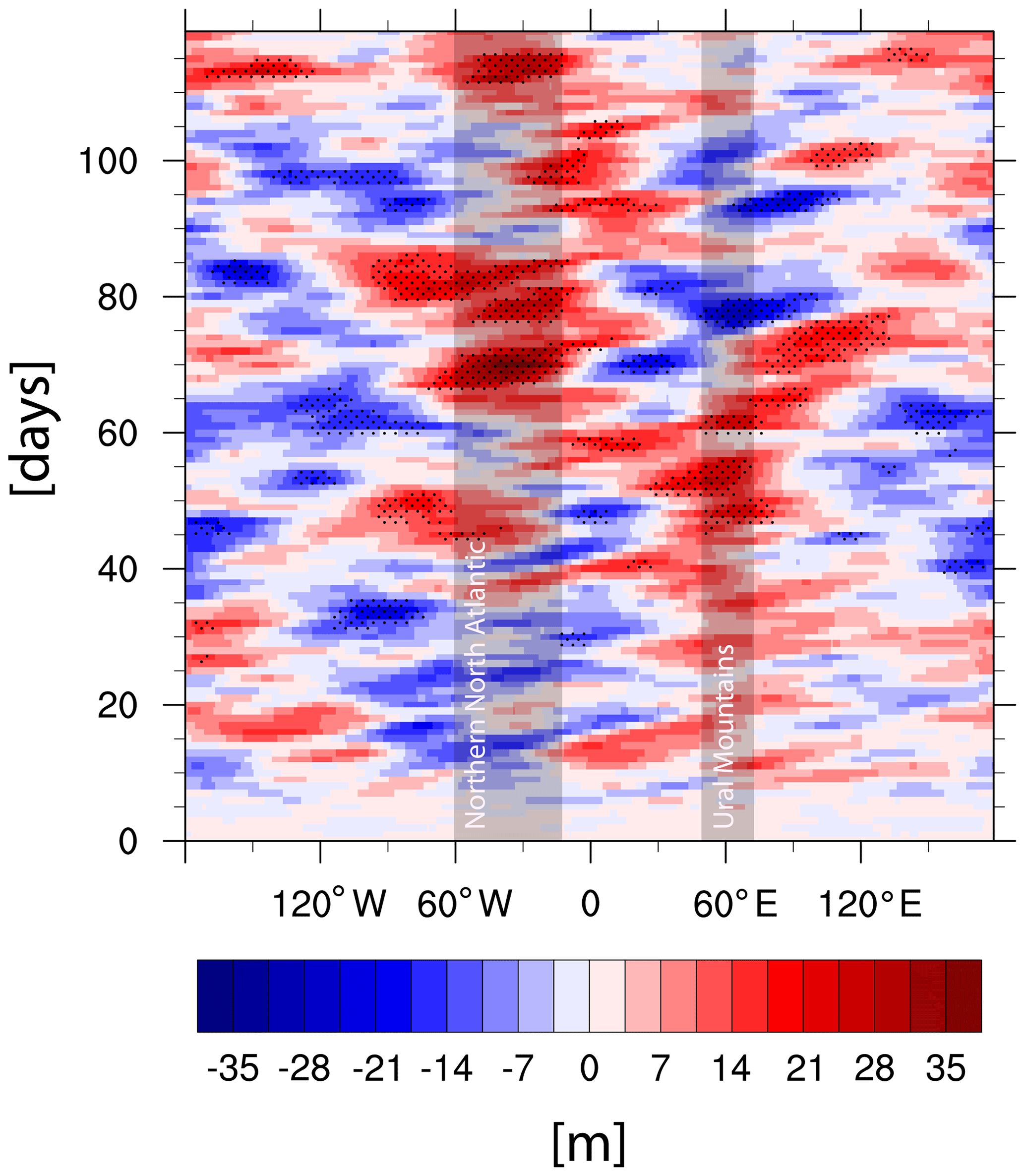
Figure 8 Hovmøller diagram of daily mean predicted 500 hPa geopotential height anomalies for the period 1901–2010 averaged for the latitude band 60–70^∘ N, as difference between high-dipole and low-dipole ASF-20C EXP ensemble means. Stippled areas represent 90 % significance. Days from 1 November are indicated on the y axis.

3.6 Non-linearities in the snow forcing impact

Two distinct non-linearities need to be considered. First, a non-linearity in the physical snow feedback: adding a few centimeters of snow in a snow–covered region will not change the radiative and thermodynamic properties of the already-snow-covered land surface substantially (due to a saturation effect), but, by contrast, removing a few centimeters of snow might remove the snow layer altogether, changing drastically the albedo and thermodynamics of the surface–atmosphere boundary. This non-linearity may be important for the Rossby wave generation as air flows over the uplifted isentropes above the snow-covered area. The non-linear effect of snow cover saturation and the impact of the relative magnitude of regional surface cooling in our experiments are addressed by Fig. 9. In years when the high-minus-low snow depth dipole EXP ensemble anomalies preceded a negative NAO anomaly (see Fig. 1d for indication of years), the December cooling anomaly over eastern Eurasia is much stronger than for the opposite case when it preceded a positive NAO anomaly. Concurrently, the formation of a Ural ridge anomaly is much more pronounced, flanked by troughs up and downstream, with positive eddy heat fluxes into the stratosphere over the Barents–Kara Sea and polar stratospheric warming. This supports the notion that adding an absolute amount of snow (in either of the two longitudinal domains) is not sufficient for the causal chain to be triggered. Instead, it is a large (in magnitude and extent) relative surface temperature impact of the additional snow that triggers the initial anomalous Rossby wave generation part of the hypothesized causal chain.

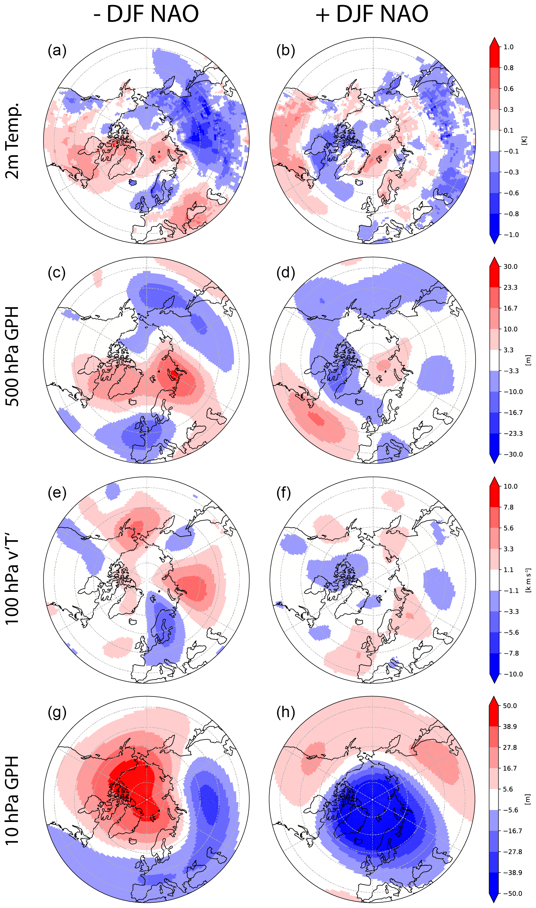
Figure 9 Climate anomaly composites of predicted December fields after which a positive snow dipole forcing preceded a negative DJF NAO signal (a, c, e, g) or a positive DJF NAO signal (b, d, f, h) (selection of years based on Fig. 1d): (a, b) 2 m temperature, (c, d) 500 hPa geopotential heights, (e, f) 100 hPa meridional eddy temperature flux and (g, h) 10 hPa geopotential heights. Anomalies are based on ASF-20C EXP high–low snow dipole ensemble mean data.

A second non-linearity is the asymmetrical role of the eastern and western domains of the snow dipole. Our subsampling of the ASF-20C EXP simulation allows us to estimate the respective roles of these two domains. Interestingly, the difference between the low snow dipole ensemble mean and the CTL ensemble mean for DJF sea level pressure (Fig. 10) reveals a much stronger response to a negative snow dipole (i.e., with high snow depths over western Russia and low snow depths over eastern Eurasia) than to the positive snow dipole (i.e., with high snow depths over eastern Eurasia and low snow depths over western Russia). The reason behind this is a combination of study design, the non-linearity of snow cover and the snow climatology of Eurasia. In Fig. 10a, we compare the effect of a very non-climatological snow depth gradient to the impact of a climatological snow depth gradient and as such get a very strong response in SLP anomalies. This comparison equalizes or reduces the snow depth gradient, and as a result very zonal flow occurs over high latitudes. In Fig. 10b, we compare the effect of a slightly increased (to the climatology) snow depth gradient to the impact of a climatological snow depth gradient and as such, in addition to the weak impact of snow cover increase, get a weak-to-non-existent surface signal out of this experimental design.

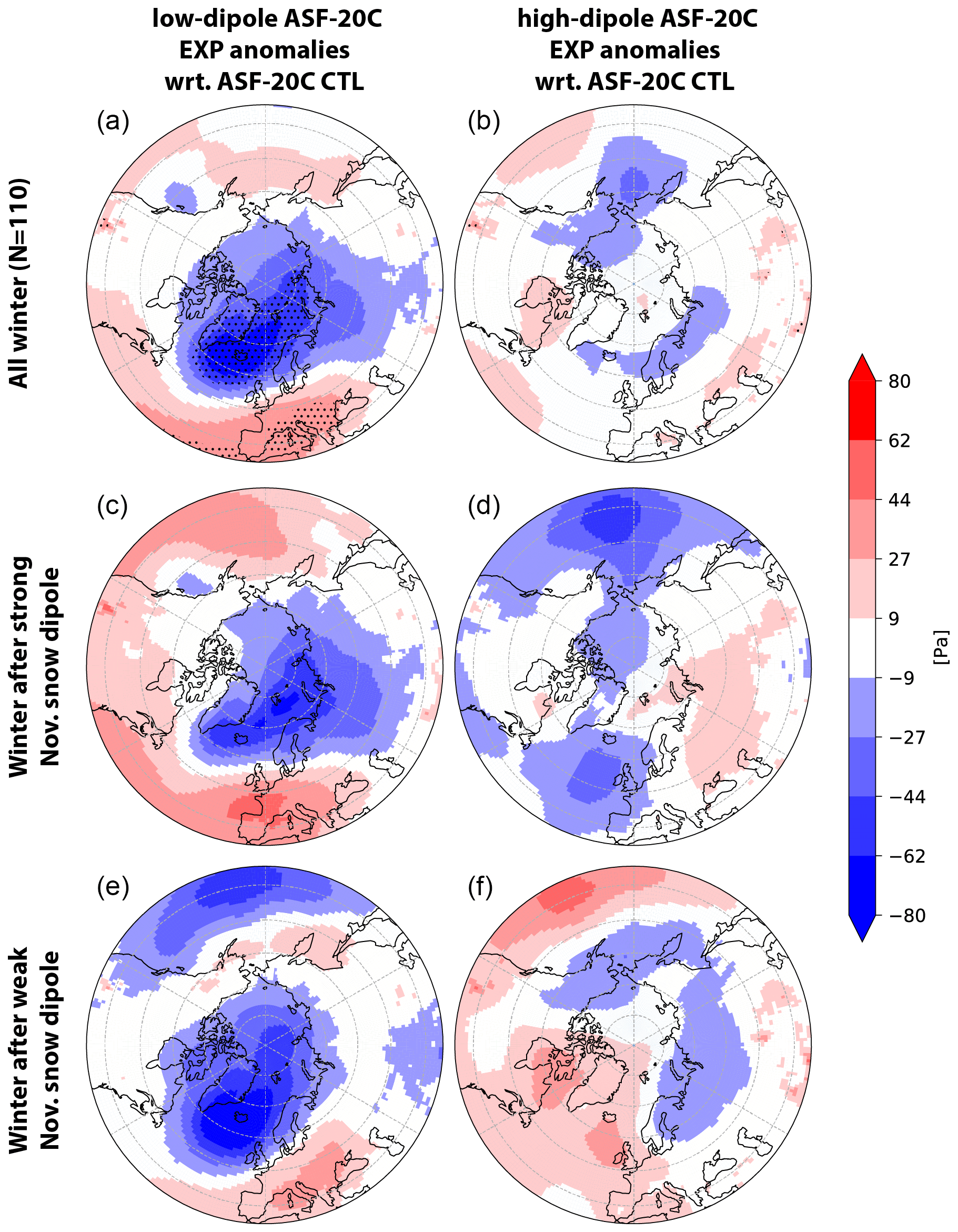
Figure 10 Mean sea level pressure [Pa] DJF anomalies for the period 1901–2010 between (a) low-dipole ASF-20C EXP ensemble mean and ASF-20C CTL ensemble mean (subsampled from 21 CTL members) and (b) high-dipole ASF-20C EXP ensemble mean and ASF-20C CTL ensemble mean (subsampled from 21 CTL members). Stippled areas represent 90 % significance. Panel (c) represents differences between low-dipole ASF-20C EXP ensemble mean and ASF-20C CTL ensemble mean DJF seasons after positive snow dipole in ERA20C 1 November snow depth (see Fig. 1a). Panel (d) as panel (c) but for the high-dipole ASF-20C EXP ensemble mean. Panels (e) and (f) the same as panels (c) and (d) but for seasons after negative snow dipole in ERA20C 1 November snow depth.

By splitting up the 110 years of ASF-20C CTL (climatology) in two batches with high or low snow depth gradient initial conditions (1 November dipole index higher or lower than 0 based on Fig. 1a), we can shed more light on those non-linearities and boost the signal of the high snow depth dipole EXP ensemble (Fig. 10c–f). If we compare the high snow dipole EXP ensemble to CTL winter after a weak west–east snow depth gradients (dipole index below 0), the anomalies show slightly elevated SLP over the northern North Atlantic (Fig. 10f), albeit in much lower magnitude than for the opposite comparison (Fig. 10e) (see Fig. S4 for snow depth anomalies). A weak snow depth gradient seems to nearly always favor zonal flow (Fig. 10d, e, f), whereas increasing the gradient needs to overcome a higher threshold due to the climatology representing a natural west–east gradient already, even before the experiment treatment shows its impact. Nevertheless, anomalies between the high snow depth dipole and low snow depth dipole EXP ensembles show the effect of an increased west–east snow depth gradient, which does in fact support the formation of more negative NAO-like states.

In other words, the relative snow depth changes in our model world are much larger in the western domain, and as such, the western domain carries most of the signal in our analysis. A simple regression analysis with the CRU DJF NAO index and ERA20C November snow depth shows a similar result (Fig. S5). We find that a linear regression model using only the eastern domain snow depth variability for explaining DJF NAO shows less significance than a model only using the western domain snow depth variability. Using the west–east gradient shows the highest significance for predicting wintertime NAO, regardless of whether we use ERA20C-derived NAO or station-based NAO.

That said, with the negative dipole corresponding to lower snow depths over the eastern domain (Mongolian Plateau and surroundings areas), our results are consistent with lessened wave fluxes into the stratosphere over this region, which is the important orographic driver of climatological upward wave fluxes in winter (White et al., 2017).

4 Discussion

We used a set of centennial ensemble seasonal hindcasts (ASF-20C) and a complementary set with perturbed land initial conditions (ASF-20C-EXP) to address some of the open questions regarding the relationship between Eurasian autumn snow cover and the state of the NAO in the following winter. Subsampling of the latter hindcast set according to the initial value (on 1 November) of a west–east snow dipole over Eurasia (Gastineau et al., 2017; Han and Sun, 2018) allowed us to determine the response over 110 winters.

The regression of stratospheric wind and temperature upon the snow dipole in ERA20C over the 1901–2010 period reveals a weakened stratospheric vortex in January and February, following a positive initial snow dipole. Even though the linear regression analysis represents a deterministic single-member approach resulting in different magnitudes and shorter response times, the seasonal evolution of the ASF-20C EXP high–low snow dipole anomalies similarly indicates a weakened polar vortex. It also supports the notion of a surface cooling over the eastern domain anchoring a Ural ridge anomaly on its western flank in December (Fig. 6e). This Ural ridge triggers an increased northward heat flux in the lower stratosphere, thereby reducing the polar vortex strength and increasing polar stratospheric temperatures. In January and February, the signal moves downwards into the troposphere where it evolves into a negative NAO anomaly. In general, these results agree with the framework proposed by Cohen et al. (2007) and the experiments with the ECMWF seasonal prediction model by Orsolini et al. (2016). The physical causal chain in our experiment is also in line with recent model studies investigating the impact of Eurasian snow on stratospheric warmings and possible surface climate anomalies (Lü et al., 2020; Cohen et al., 2021). However, it should be highlighted that the absolute ensemble mean, time-average SLP signal, diagnosed as the conditional composite difference in ASF-20C EXP, is very small – less than 1 hPa. As mentioned before, this represents only a small fraction of the interannual SLP variability in the Euro-Atlantic region. Nevertheless, for single realizations of winter forecasts, this impact can be much higher. By design, we excluded the impact of sea ice on the NAO evolution, since SSTs and sea ice stay the same through time in all EXP members. We checked for significant tropical precipitation patterns in the high-minus-low anomalies for November and December as potential co-variates in driving an DJF NAO signal but found no coherent significance across tropical latitudes. As such, we exclude tropical rainfall as first-order driver behind the EXP NAO response.

The role of the Ural ridge in the snow cover → NAO causal chain has been discussed and analyzed in several recent studies (Peings, 2019; Santolaria-Otín et al., 2021). Here we find that the Ural ridge is a pre-condition of predicted negative NAO winters in ASF-20 CTL (Fig. S6), together with a cold 2 m temperature anomaly in eastern Russia and a cold stratospheric polar vortex displaced over Eurasia, downstream of the Ural ridge. However, these initial conditions are subtracted out in the ASF-20C EXP high–low snow dipole composite difference, and we find that the composite difference indicates a reinforced Ural ridge (Fig. 6e). We find the mid-troposphere Ural ridge is reinforced only at the end of November going into December, which precedes the formation of a North Atlantic ridge that prevails until February (Fig. 8). This result indicates that the snowpack does indeed play a feedback role (see also Orsolini et al., 2016). Thus, we propose that the relation between the Ural ridge and Eurasian snow cover consists of a mutual interaction: the circulation anomaly associated with a pre-existing Ural ridge shovels cold polar air southwards along its eastern flank, allowing for a deeper snowpack to form over eastern Eurasia. In addition to this process (Fig. 9c), our analysis reveals that the snow cover anomaly reinforces the Ural ridge, allowing for increased wave flux into the stratosphere. This location of a tropospheric ridge interferes constructively with climatological stationary wave-1 and wave-2 patterns (Garfinkel et al., 2010) and seems to be key for a skilled forecast of the polar winter stratosphere (Portal et al., 2021).

Furthermore, the high-minus-low composite highlights a subpolar North Pacific surface and mid-tropospheric low-pressure anomaly that appears first in December and remains throughout all of DJF (Figs. 6f, g, i and 10). The generation of this circulation feature was pointed out by previous studies (Orsolini and Kvamstø, 2009; Garfinkel et al., 2010, 2020) and has been attributed to an enhanced vertical propagation of Rossby waves into the stratosphere downstream of the cooled Eurasian land mass.

Subsampling of the experimental multi-decadal historical hindcasts (ASF-20C EXP) highlighted an interdecadal variability and non-stationarity of the snow dipole impact, despite the canceling out of common boundary forcings such as SSTs in the composite difference. The configuration of our experiment does not allow us to explain this behavior completely; however, we can address some possible reasons. A potential influence on the decadal variability of the snow cover impact might be the precursory climate system state, promoting or counteracting the tendency for the (perturbed) snow forcing towards a given NAO state.

Surprisingly, the positive snow dipole forcing tends to favor a negative NAO signal when the climate system is “tuned” for a positive winter NAO in ERA20C, for example when high ERA20C Barents–Kara Sea ice extent and La Niña SST conditions prevail (Fig. S7). This supports the idea of a clear and strong snow impact when the relative cooling anomaly in eastern Eurasia is relatively strong and the climate state is preconditioned to a rather positive NAO-like condition. This might explain the strong positive NAO anomaly during the early 20th century Arctic warming in Fig. 1d: the period 1920–1940 was characterized by a strong positive mid-tropospheric high anomaly from northern Europe to east Siberia (Wegmann et al., 2017a). We find that the 500 hPa anomalies between high and low snow composites show only a weak-to-non-existent Ural ridge for the period 1921–1940, when compared to, e.g., 1991–2010 (Fig. S8). On the contrary, increased snow in an already-snow-covered eastern Eurasia will not provide the same response as the pre-existing anomalies favored by other background conditions. Rather, strong non-linearities seem to occur, which is reasonable given the non-linear thermodynamic and radiative impacts of a deeper snowpack.

On that note, we find that the relative magnitude of regional cooling compared to the existing climate state in our experiments is of crucial importance. In years when the high–low snow dipole anomalies preceded a negative NAO, the December cooling anomaly over eastern Eurasia is much stronger than for the opposite case (Fig. 9). Moreover, we found that in our model experiment a negative snow dipole forcing leading to a positive NAO signal has a much larger relative impact compared to the positive snow dipole resulting in a negative NAO signal, which is due to the much stronger changes in surface forcing that we impose with the negative snow dipole ensemble. Moreover, due to the Eurasian snow climatology, a similar level of snow depth variability in the western domain will have higher impacts on the tropospheric variability. In our experimental setup, a weak snow depth gradient from west to east allows for a rather zonal circulation in the following months, with no subsequent stratospheric warming signal. Distinct model experiments are needed to understand the atmospheric feedbacks of these configurations better.

As such, we find that the main driver for the proposed snow–stratosphere linkage is a large relative impact of the additional snow depth in terms of surface temperatures as well as a strong west–east snow depth gradient. Generally, our results further highlight the importance behind the land memory effect discussed by Nakamura et al. (2019) as well as Tyrrell et al. (2019), who argue for a delayed impact of snow cover via soil and surface temperatures.

Nevertheless, we are limited in analyzing the impact of co-variability in the climate system over the span of the 110-year period. Additional experiments are needed to investigate the role of climate state precursors and memory effects influencing the seasonal predictions.

5 Summary and conclusion

Centennial seasonal ensemble hindcasts were used to examine the impact of a realistically increased November Eurasian west-to-east snow depth gradient on the boreal winter climate evolution. We found evidence for the manifestation of a negative NAO signal after a strong, positive November west-to-east snow cover dipole via surface cooling, increased Ural blocking and subsequent stratospheric warming (although evolution toward a positive NAO state was also observed but less frequently, especially for NAO extremes). Including 110 years of natural Earth system variability increases the confidence in the proposed physical mechanisms behind cryospheric drivers of atmospheric variability and decreases the probability of random co-variability between snow cover and DJF NAO. Our results hence support previous hypotheses and statistical studies. The absolute surface impact was found to be small in our experimental setup, with interdecadal variability and ensemble averaging reducing the magnitude of individual events. We found the impact of our snow forcing to be strongest for climate states that will allow the snow forcing to exert a strong surface cooling.

Future studies need to address the interplay between different Earth system components in coupled seasonal prediction experiments. How important the background conditions of the climate system are before the initialization of the forecasts needs to be investigated further. Furthermore, allowing higher magnitude snow forcing (e.g., perturbing initial land states over a longer range than the neighboring 10 years as in this study) might result in stronger stratospheric and surface signals.