Dynamical and surface impacts of the January 2021 sudden stratospheric warming in novel Aeolus wind observations, MLS and ERA5

Major sudden stratospheric warmings (SSWs) are extreme dynamical events where the usual strong westerly winds of the stratospheric polar vortex temporarily weaken or reverse and polar stratospheric temperatures rise by tens of kelvins over just a few days and remain so for an extended period. Via dynamical modification of the atmosphere below them, SSWs are believed to be a key contributor to extreme winter weather events at the surface over the following weeks. SSW-induced changes to the wind structure of the polar vortex have previously been studied in models and reanalyses and in localised measurements such as radiosondes and radars but have not previously been directly and systematically observed on a global scale because of the major technical challenges involved in observing winds from space. Here, we exploit novel observations from ESA's flagship Aeolus wind-profiler mission, together with temperature and geopotential height data from NASA's Microwave Limb Sounder and surface variables from the ERA5 reanalysis, to study the 2021 SSW. This allows us to directly examine wind and related dynamical changes associated with the January 2021 major SSW. Aeolus is the first satellite mission to systematically and directly acquire profiles of wind, and therefore our results represent the first direct measurements of SSW-induced wind changes at the global scale. We see a complete reversal of the zonal winds in the lower to middle stratosphere, with reversed winds in some geographic regions reaching down to the bottom 2 km of the atmosphere. These altered winds are associated with major changes to surface temperature patterns, and in particular we see a strong potential linkage from the SSW to extreme winter weather outbreaks in Greece and Texas during late January and early February. Our results (1) demonstrate the benefits of wind-profiling satellites such as Aeolus in terms of both their direct measurement capability and use in supporting reanalysis-driven interpretation of stratosphere–troposphere coupling signatures, (2) provide a detailed dynamical description of a major weather event, and (3) have implications for the development of Earth-system models capable of accurately forecasting extreme winter weather.

1 Introduction

Sudden stratospheric warmings (SSWs) are some of the most dramatic dynamical events in the entire atmospheric system. Over just a few days, temperatures in the winter polar stratosphere can rise by as much as 50 K, while the circumpolar wind jet which usually separates the cold polar stratosphere from midlatitudes dramatically reduces in speed and, at many heights and locations, can even reverse. These dynamical changes have major effects on both weather and longer-scale atmospheric processes: in addition to direct local changes to polar ozone and other chemistry (Tao et al., 2015; Manney et al., 2015b, a; Safieddine et al., 2020), the altered wind patterns couple outwards to the broader atmospheric system with significant and widespread ramifications (e.g. Pedatella et al., 2018). In particular, SSWs can trigger extreme winter weather events at ground level in the heavily populated midlatitude regions of North America and Europe, with significant social, safety and economic impacts (Kretschmer et al., 2018; Charlton-Perez et al., 2021; Domeisen et al., 2020; Hall et al., 2021).

The collapse of the circumpolar wind jet is arguably the most important factor affecting how SSWs interact with the broader Earth system. Reflecting this importance, the most broadly used definition of a major SSW is wind-based rather than temperature-based: specifically, a major SSW is often defined as a wintertime event in which the zonal mean at 60^∘ and 10 hPa reaches zero (Charlton and Polvani, 2007). However, direct observations of the vortex winds are extremely technically challenging to make. While wind speed measurements using in situ radiosondes and ground-based remote-sensing techniques such as lidar and radar are routinely made at many sites, the point-based nature of these techniques inherently limits their ability to characterise the large-scale changes SSWs induce in wind patterns.

Due to these observational limitations, the vast majority of recent research on how SSWs affect winds above the lowest layers of the atmosphere has been carried out using models, reanalyses and winds inferred from other measured variables such as temperature. While these tools have proven highly effective and have significantly advanced our ability to predict winter weather around SSW events, they are not true measurements of wind speed – instead, they infer the wind state through a combination of numerical computation and/or how the wind affects and is affected by other atmospheric parameters.

Here, we exploit data from the European Space Agency's (ESA) flagship Aeolus satellite mission to directly measure SSW effects on winds in the lower-stratospheric vortex for the first time. Launched in mid-2018, Aeolus is the first satellite instrument capable of systematically and directly measuring winds in the global free troposphere and lower stratosphere and as such provides a unique window on how SSWs affect winds throughout the lower and lower to middle atmosphere. While Aeolus does not routinely measure winds as high as the 10 hPa (∼32 km) level typically used to diagnose the presence of a major SSW, measurements are available from the surface to ∼24 km (30 hPa). This height range allows us to study both a large fraction of the direct polar vortex changes induced by SSWs and also examine how these changes affect winds at all heights below.

In the atmosphere, in addition to Aeolus data we also use temperature observations and geostrophic wind estimates inferred from the Microwave Limb Sounder on NASA's Aura satellite and wind, temperature and geopotential height (GPH) output from the European Centre for Medium-Range Weather Forecasts' ERA5 reanalysis. We also investigate the potential surface impacts of the SSW, using temperature, snow cover extent and GPH data from ERA5.

We first describe the Aeolus, MLS and ERA5 data in detail in Sect. 2. We next place the January 2021 SSW in its broader climatological context in Sect. 3, using ERA5 and MLS data for all winters since MLS launched in 2004. Section 4 then describes the evolution of the 2021 event specifically using zonal-mean Aeolus and MLS observations. We follow this with a brief discussion of the nature of the event in terms of vortex summary metrics in Sect. 5, before moving on to examine sub-zonal variability in Sect. 6, both in terms of Aeolus wind and MLS GPH measurements. Finally, in Sect. 7 we study surface weather impacts temporally associated with the SSW, before discussing our results and drawing conclusions in Sect. 8.

2 Data

2.1 Aeolus

Aeolus is ESA's fifth Earth Explorer mission (Stoffelen et al., 2005; ESA, 2008; Reitebuch, 2012; Stoffelen et al., 2020), which launched in mid-2018. The Aeolus satellite itself is a polar orbiter, in a 320 km sun-synchronous dawn–dusk 97^∘ inclination orbit with Equator-crossing local solar times of 06:00 and 18:00 LT in the descending and ascending node respectively. This orbit approaches each pole 15.6 times per day and thus provides a platform well suited to characterising polar atmospheric dynamics.

The satellite carries a single primary payload, the Atmospheric Laser Doppler Instrument (ALADIN). This is a Doppler wind lidar designed to measure winds, aerosol and cloud in the bottom 30 km of the atmosphere. A 335 nm laser directed at 35^∘ off-nadir and 90^∘ off-track measures both molecular (Rayleigh) and aerosol (Mie) backscatter. We use baseline-12 Rayleigh data, which has a vertical resolution ∼0.5–2 km depending on scanning mode and a horizontal (along-track) resolution of ∼90 km for the profiles studied. Following corrections for hot pixels, telescope-temperature-dependent biases and a longitude-dependent bias, a mean instrument bias ≲0.6 m s⁻¹ has been estimated for these data relative to northern-midlatitude radiosondes and to numerical weather prediction (NWP) models (Chanin et al., 1989; Weiler et al., 2021; Rennie et al., 2021; Martin et al., 2021). For quality control, we require that the horizontal line-of-sight (HLOS) error estimate set by the retrieval is <8 m s⁻¹ and that the data are not cloud-contaminated (i.e. Rayleigh clear only).

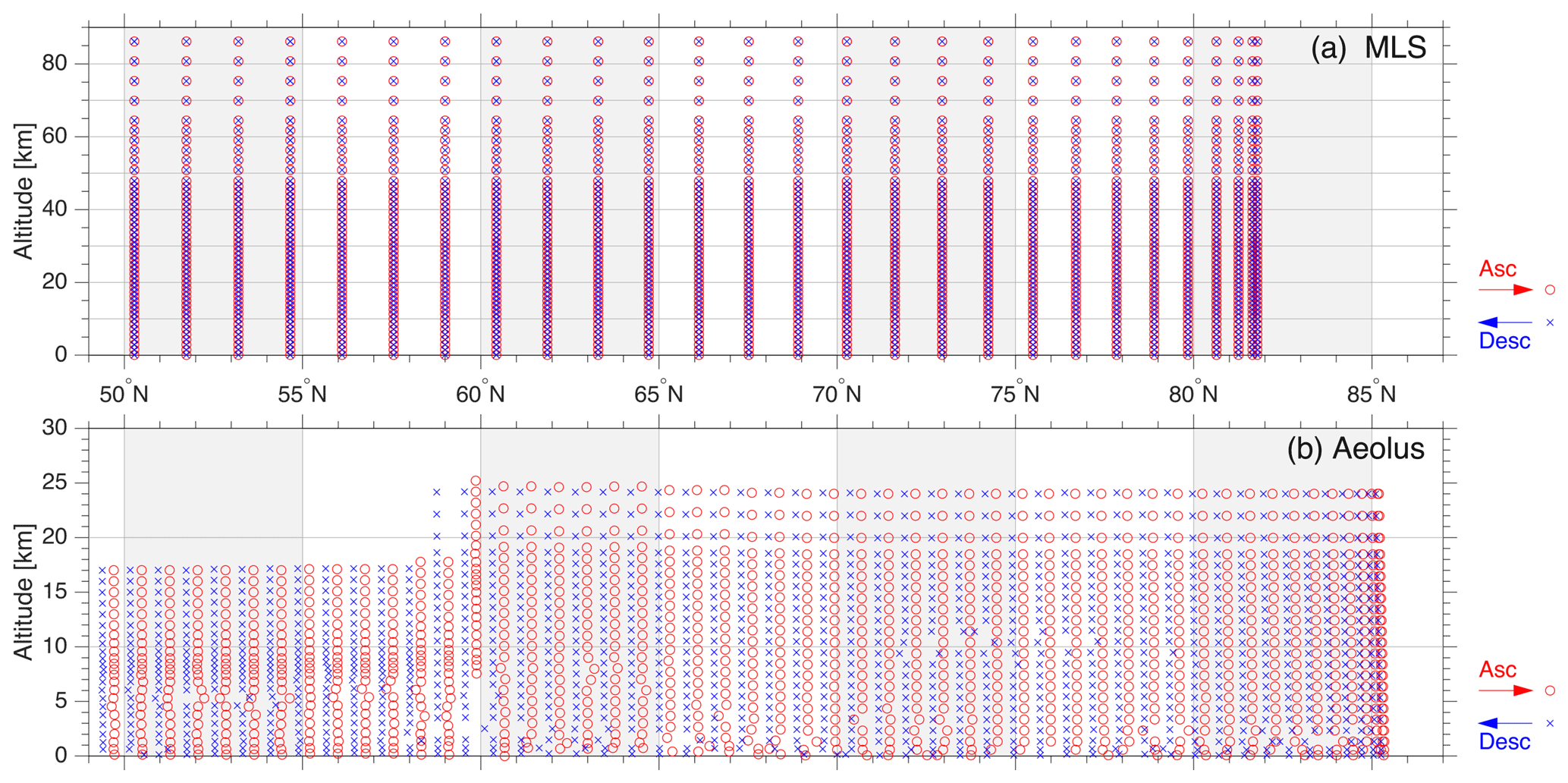
Figure 1 Illustration of (a) MLS and (b) Aeolus measurement spacing in northern polar regions. On each panel, the first complete part-orbit crossing poleward of 60^∘ N on 5 January 2021 is shown – this orbit is typical for those during our study. Red circles indicate measurements on the latitude-ascending node of the orbit and blue crosses measurements on the latitude-descending node of the orbit. Data are shown on their retrieval grids, which do not inherently correspond to the true resolution of the measurement. Note in particular the sharp change in height coverage at around 60^∘ N in Aeolus data.

Aeolus measures HLOS winds relative to the lidar boresight¹. However, atmospheric dynamics is usually described in a resolved zonal/meridional framework, and thus we convert our observations into this frame. Appendix A describes this conversion and the underlying assumptions we make to carry it out.

Additionally, Aeolus' vertical scan pattern changes regularly. While the instrument is capable of measuring wind speeds at heights up to 30 km, in practice the height range and spacing of individual profiles varies to accommodate both specific science objectives and a broader numerical weather prediction role. As operated at the time of data collection for this study, the maximum altitude of the Aeolus wind dataset was typically lower equatorward of 60^∘ N than it was poleward. This is illustrated by Fig. 1b, which shows the spacing in height and latitude of Aeolus measurements for the first complete orbit on 5 January 2021 poleward of 50^∘ N; this orbit is broadly typical of the study period from mid-November onwards. As such, to provide a uniform spatial average for all comparisons, throughout this study we average over the region 60–65^∘ N in all analyses intended to characterise atmospheric dynamics and structure around 60^∘ N, to ensure a fair comparison at all heights.

2.2 Microwave limb sounder

We use v5.0 Level 2 data from the Microwave Limb Sounder on NASA's Aura satellite. Launched in 2004, Aura flies in a sun-synchronous polar orbit with Equator-crossing times of 01:30 and 13:30 LT. MLS uses a limb-sounding technique to measure atmospheric microwave emissions in five spectral bands (Waters et al., 2006). Temperature and pressure are obtained from the 118 and 239 GHz bands, retrieved over the range 261–0.001 hPa (∼10–100 km). Vertical resolution is variable, monotonically improving from 5 km to 3.6 km over the height range 10–25 km before monotonically worsening again to 5 km at 40 km (see Fig. 1a for sampling and Fig. 6a of Wright et al., 2016 for resolution). This is finer than most nadir-sounding instruments but significantly coarser than Aeolus. In the upper troposphere and lower stratosphere (UTLS), along-track resolution is ∼170 km, estimated temperature precision is ∼0.6 K and estimated temperature accuracy is −2.5–+1 K (Livesey et al., 2020). Figure 1a shows the spacing of these measurements for a typical orbit.

We also use MLS geopotential heights (GPH) and geostrophic winds. The GPH product is retrieved from the 118 and 234 GHz O₂ spectral bands (Livesey et al., 2020), using the methodology described by Schwartz et al. (2008), and primarily derives from MLS temperatures (Livesey et al., 2006). In the height range studied, the product used has a vertical resolution of 4–12 km, a precision of 20–110 m and an accuracy error of 0–150 m, with the less precise/poorer resolution extrema more typical of the top of the column.

We compute geostrophic winds from these GPH data, binned onto on a $\mathrm{5}{}^{\circ }\times \mathrm{20}{}^{\circ }$ latitude–longitude grid independently for each MLS pressure level and day. We use the relation $u=-(g/f)\mathrm{d}Z/\mathrm{d}y$, where Z is GPH, y is the meridional distance between measurement bins, f is the Coriolis parameter and g is the acceleration downwards due to gravity (assumed to be 9.81 m s⁻¹). Values estimated on this grid are then bilinearly interpolated back to the instrument scan track, again for each pressure level and day independently, in order to provide a spatial weighting roughly equivalent to that for MLS temperature. This choice is made to provide better comparability between analyses produced using the temperature, GPH and wind datasets.

Due to this significant spatiotemporal averaging, these geostrophic winds are very coarse relative to Aeolus. The calculation also inherently relies on an assumption of atmospheric geostrophy. In our study region, we expect the difference between geostrophic and true wind to increase with height due to the driving effects of processes such as gravity wave breaking, and MLS wind estimates at high altitudes in particular should be treated with caution. We use only zonal-mean zonal MLS wind in this study, which we validate against Aeolus, reanalysis and operational analysis zonal-mean zonal winds in the troposphere and stratosphere in Sect. 2.4.

MLS data are unavailable for a large fraction of 24 December 2020, and the collected data for this day exhibit a markedly different zonal mean and height dependence when compared to the surrounding days. This difference is due to the partial data coverage rather than true geophysical differences. Accordingly, to remove the effect of this anomalous day from our analyses, this day has been replaced in all analyses by the mean of 23 and 25 December 2020.

2.3 ERA5 and ECMWF operational analyses

We use ERA5 reanalysis output (C3S, 2021; Hersbach et al., 2020) and European Centre for Medium-Range Weather Forecasting (ECMWF) operational analysis (hereafter “OpAl” for brevity). OpAl is only used in Sect. 2.4, where its zonal-mean zonal wind is shown to be almost identical to ERA5 at the heights and times considered in the zonal mean, and in the rest of the study we use ERA5 only.

ERA5 is a fifth-generation reanalysis product produced by the ECMWF. OpAl is broadly similar in concept but uses a current version of the assimilative IFS weather model – for this study, IFS Cycle 47r1 – rather than a fixed version as with ERA5, which uses IFS cycle 41r2, a 2016 version of the operational model. Furthermore, OpAl assimilates Aeolus data, while ERA5 does not. Therefore, ERA5 data are independent of Aeolus, while OpAl data are constrained by it. ERA5 is, however, constrained by other data sources, including in this altitude range by aircraft, radiosondes, and satellite radiance and bending angle data and therefore should reflect broadly the same geophysical state.

We use several forms of ERA5 data.

• In Figs. 2–5, we use temperature and zonal and meridional wind fields stored on 137 model levels spaced non-uniformly from the surface to 0.01 hPa. These have been downsampled to a spatial resolution of 1.5^∘ and to a 3 h time resolution to facilitate analysis of comparatively large data volumes.

• In Figs. 6, 10 and 11 we use GPH stored on 37 pressure levels spaced non-uniformly from the surface to 1 hPa (∼48 km altitude), with daily (specifically, midnight UTC) temporal resolution and at the full spatial resolution of 0.25^∘.

• In Fig. 10 we use the daily snowfall field, also on a 0.25^∘ grid.

• In Figs. 10 and 11, we use the daily midnight 2 m altitude temperature field, also on a 0.25^∘ grid.

Like all reanalyses and models, these datasets inherently exhibit meaningful differences from the observed atmospheric state, both systematic and random, particularly at short length scales and high altitudes (e.g. Long et al., 2017). Although systematic assessments of high-altitude wind accuracy at the global scale are challenging to produce due to the scarcity of suitable observations, an assessment of temperature relative to limb sounder data suggests that, at the altitudes considered here, pointwise differences from observations were generally small, with typical pointwise root-mean-square temperatures differences from limb sounder observations < 2 K and Pearson linear correlations > 0.95 (Wright and Hindley, 2018).

2.4 Geostrophic wind cross validation

Figure 2 shows time series of zonal mean zonal wind speed $\stackrel{\mathrm{‾}}{u}$ derived from Aeolus (blue), ERA5 (pink dashed), OpAl (red), and MLS (orange), all averaged over the 60–65^∘ N latitude band and shown at the 32 km (Fig. 2a), 22 km (Fig. 2b) and 15 km (Fig. 2c) altitude levels. An altitude of 32 km represents approximately the usual 10 hPa pressure level at which SSWs are defined but is not measured by Aeolus; 22 km is the highest altitude measured by Aeolus for the great majority of the period studied (commencing in mid-November), and 15 km is the highest altitude level at which Aeolus measurements are made for the entire period studied (i.e. including early November). While this figure shows clear evidence of the large dynamical changes due to the SSW that are the focus of our study, our primary aim here is to assess the consistency or otherwise of these four datasets, and we therefore reserve detailed discussion of the dynamical situation to Sect. 3 onwards.

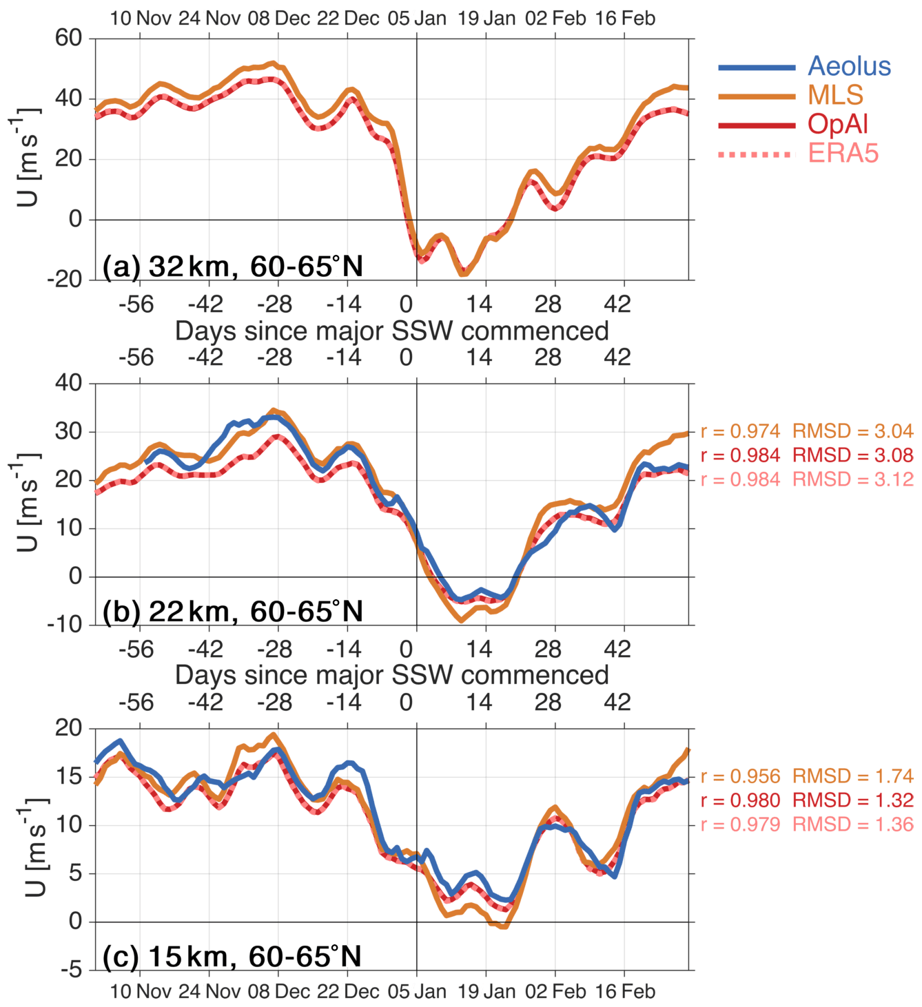
Figure 2 Daily-mean time series of zonal mean Aeolus HLOS-projected u, MLS geostrophic u, ERA5 u and ECMWF operational analysis u at (a) 32 km [∼10 hPa] (b) 22 km and (c) 15 km altitude, averaged over the 60–65^∘ N latitude band and stationary-boxcar-smoothed 3 d to account for variable spatial coverage of satellite data. For each non-Aeolus datasets, the Pearson linear correlation with root-mean-square difference (in m s⁻¹) from the Aeolus time series is shown, computed over all days for which both datasets have coverage in that time series.

Very close agreement is seen between the four zonal mean time series, with Aeolus-relative correlations > 0.95 in all cases and root-mean-square differences of <3.2 m s⁻¹. Good visual agreement is also seen between MLS and reanalysis/operational analysis in the 32 km data. Based on this comparison, we conclude that MLS $\stackrel{\mathrm{‾}}{u}$ is sufficiently robust in the zonal mean for use in our study, at least at these altitudes and latitudes; this reinforces the results of previous studies that have used these data to understand SSW dynamics (e.g. Manney et al., 2008, 2009, 2015b; Smith et al., 2017; Harvey et al., 2018, 2019). We further conclude that ERA5 and OpAl data in the zonal mean are sufficiently similar that they can be used interchangeably for our purposes; since some later analyses involve comparisons to climatology, we therefore use ERA5 throughout the remainder of this study for consistency.

Some differences are seen between the datasets, but these differences are small – this is consistent with the high quality of the datasets and very large spatial averaging implicit in taking a zonal mean. At the 22 km level, Aeolus typically exhibits more positive values of u before and during and lower values of u after the SSW relative to the ECMWF products, while MLS has more positive u both before and after but more negative u during the SSW. At the 15 km level, Aeolus generally has more positive u than the ECMWF products except for brief periods, while MLS u is again more positive before the SSW and more negative during. Closer investigation of these differences, including their geographic structure at spatial scales below the zonal mean, is beyond the scope of our study but may be a fruitful path for future work.

3 The climatological context of the 2021 SSW

Figure 3 shows MLS zonal mean temperature $\stackrel{\mathrm{‾}}{T}$ (Fig. 3a, c and e) and ERA5 $\stackrel{\mathrm{‾}}{u}$ (Fig. 3b, d, f and g) analysed relative to a climatology produced using all winters between 2004/05 and 2019/20, i.e. the period since MLS began collecting data. $\stackrel{\mathrm{‾}}{T}$ has been averaged across the entire region poleward of 60^∘ N to provide an estimate of the mean polar context (but note that MLS data only extend to 82^∘ N), while $\stackrel{\mathrm{‾}}{u}$ has been averaged zonally across the 60–65^∘ N latitude band to focus on the strength of winds in regions closer to the nominal edge of the polar vortex under undisturbed conditions.

Figure 3 Context of the January 2021 SSW in relation to a 2004/05–2019/20 climatology of zonal mean (a, c, e) MLS temperatures and (b, d, f, g) ERA5 zonal winds at (a, b) 32 km, (c, d) 22 km, (e, f) 15 km and (g) 5 km altitude. Grey shading shows the climatological distribution, with the 0th, 18th, 50th, 82nd and 100th percentiles (i.e. non-parametric equivalents of the range, median, and first and second standard deviations) emphasised by solid grey lines. Red line shows winter 2020/21 within this context.

We show data at the (a, b) 32 km, (c, d) 22 km, (e, f) 15 km and (g) 5 km levels; the first three have been selected for consistency with Fig. 2, with the fourth added to provide tropospheric context. 2020/21 is highlighted in red. Grey shading illustrates the spread of the 2004/05–2018/19 climatology, with shades of grey indicating specific positions in the climatology and with the 0th, 18th, 50th, 82nd and 100th percentiles (i.e. non-parametric equivalents of the range, median, and first and second standard deviations) emphasised by solid grey lines. For a 15-winter climatology such as this, the regions above and below the 18th and 82nd percentiles respectively represent three individual winters each, while the region between these bounds represents the remaining nine winters. There have been two previous early-January major SSWs since 2004 (Butler et al., 2017), reaching zero $\stackrel{\mathrm{‾}}{u}$ at 10 hPa, 60^∘ N on 6 January 2013 and 2 January 2019 respectively. As these previous SSWs contribute strongly to the relatively short climatological period shown, we therefore do not inherently expect the 2021 SSW to automatically exceed the shaded range, although given the heterogeneity of dynamical states and start dates within the observed record of SSWs it sometimes does so.

$\stackrel{\mathrm{‾}}{T}$ before early December is at or below the centre of the climatological range at the 32 km level and below it at the 22 and 15 km levels, only rarely approaching the 50th percentile at the lower two heights. $\stackrel{\mathrm{‾}}{u}$ during this period at all altitudes is noticeably above climatology to a similar degree as $\stackrel{\mathrm{‾}}{T}$ is below ≥15 km. $\stackrel{\mathrm{‾}}{u}$ at 5 km show no consistent trend during this period, varying for example from an all-climatology maximum in early November to a near-minimum 2 weeks later.

From early December to around 1 January at heights ≥ 15 km, $\stackrel{\mathrm{‾}}{T}$ starts to rise slightly, while $\stackrel{\mathrm{‾}}{u}$ drops. Around 1 January, the rise in $\stackrel{\mathrm{‾}}{T}$ rapidly accelerates, moving from the centre of the climatological distribution to climatology-topping values by 5 January and remaining at this level for around 18 d. $\stackrel{\mathrm{‾}}{u}$ during this period reaches a climatology-relative minimum for this time period. After this maximum (minimum) in $\stackrel{\mathrm{‾}}{T}$ ($\stackrel{\mathrm{‾}}{u}$), temperatures (winds) start to slowly return to climatology; this return is a mixture of falling temperatures during 2021 and a rise in the climatological median and range (albeit partly due to the presence of later SSWs in other years within the data record), and vice versa for $\stackrel{\mathrm{‾}}{u}$. After the first week of February, temperatures and winds at these altitudes remain within the central region for the remainder of the study period.

At the 5 km level, $\stackrel{\mathrm{‾}}{u}$ shows no major response to the first minimum of the SSW in early January. A local minimum in $\stackrel{\mathrm{‾}}{u}$ is seen around day 35 of the year at the 5 and 15 km levels, which may be associated with a second $\stackrel{\mathrm{‾}}{u}$ minimum associated with the SSW shown later in our study (Figs. 5 and 8).

4 Zonal-mean winds and temperatures in the winter 2020/21 sudden stratospheric warming

Figures 4 and 5 show MLS- and Aeolus-derived $\stackrel{\mathrm{‾}}{u}$ and $\stackrel{\mathrm{‾}}{T}$ for winter 2020/21, again averaged over the region poleward of 60^∘ N for temperatures and over the 60–65^∘ N latitude band for winds. Temperatures are shown as zonal mean anomalies $\stackrel{\mathrm{‾}}{T_{\mathrm{a}}}$ from the mission-to-date day-of-year median; this is intended to both remove the strong vertical dependence of temperature on height and contextualise the data in the historical record. Figure S1 in the Supplement shows absolute measured temperatures on the same axes as Figs. 4a and 5a for context.

For Aeolus $\stackrel{\mathrm{‾}}{u}$ (Fig. 5b), the bottom few kilometres represent an incomplete zonal mean (for example, Greenland's topography reaches maximal altitudes of >3 km in this latitude band) and a more technically challenging measurement than at higher altitudes. Thus, altitudes below 2 km have been omitted completely, and altitudes below ∼5 km should be treated with caution, although we note that case studies and validation campaigns using Aeolus data have shown plausible and consistent results at even the lowest altitudes (e.g. Lux et al., 2020; Witschas et al., 2020; Banyard et al., 2021).

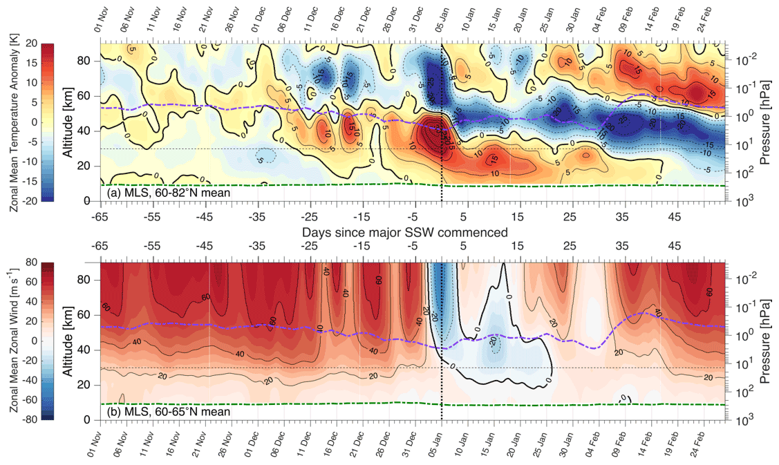
Figure 4 MLS-derived (a) 60–90^∘ N mean temperature anomalies; (b) 60–65^∘ N mean geostrophic zonal winds over the height range 0–90 km for winter 2020/21. Mean tropopause (stratopause) height derived from ERA5 is shown as a dot-dashed green (purple) line. Vertical dotted line indicates the date at which 10 hPa winds reversed and the SSW became defined as major. Horizontal dashed line indicates the top of Fig. 5. Times are shown as days relative to 5 January 2021 on the centre-figure axes and as dates on the outer-figure axes, with minor ticks indicating a step of 1 d.

Figure 5 (a) MLS-derived 60–90^∘ N mean temperature anomalies; (b) Aeolus-derived 60–65^∘ N mean projected zonal winds for winter 2020/21, for altitudes 0–30 km. Mean tropopause height derived from ERA5 is shown as a dot-dashed green line. Vertical dotted line indicates the date at which 10 hPa winds reversed and the SSW became defined as major. Numbered boxes on the horizontal axis of (b) are used to guide discussion from Sect. 6 onwards. Times are shown as days relative to 5 January 2021 on the centre-figure axes and as dates on the outer-figure axes, with minor ticks indicating a step of 1 d.

Aeolus data are shown at a 2 km by 1 d resolution, as described in Appendix A. For MLS, daily time bins are also used, but the width of the height bins is set to 4 km at altitudes below 55 km altitude and 6 km above. The green and purple dot-dashed lines overlaid on the data show the zonal-mean temperature-tropopause and stratopause height at 60^∘ N for that day, derived from ERA5 as described by Wright and Banyard (2020) and France et al. (2012) respectively. A wider latitude range (50–70^∘ N) was also tested for Aeolus winds; results were broadly similar but with a deeper and longer-lasting period of negative zonal winds at the top of the measured column following the SSW.

4.1 Stratospheric and mesospheric context

We consider first the broader-scale picture provided by Fig. 4. Polar-cap temperature (Fig. 4a) is around the median for this time of year in November, with $\left|\stackrel{\mathrm{‾}}{T_{\mathrm{a}}}\right|<$5 K at all heights. $\stackrel{\mathrm{‾}}{T_{\mathrm{a}}}$ is small and negative in the mid-stratosphere and mid-mesosphere and small and positive around the stratopause and (in early November) in the upper mesosphere. The small local maximum around the stratopause is likely due to interannual stratopause height variability rather than a substantive difference. The zonal mean zonal wind at 60–65^∘ N during this period (Fig. 4b) is generally large and positive throughout the stratosphere and mesosphere.

From around 1 December, mid-stratospheric $\stackrel{\mathrm{‾}}{T_{\mathrm{a}}}$ dips to more than 5 K below climatology for a few days, while mesospheric $\stackrel{\mathrm{‾}}{T_{\mathrm{a}}}$ becomes anomalously positive up to above 80 km altitude. These signals, while small, mark the start of a period of significant disruption at all heights, associated with a steady drop in stratopause height. Throughout early December, stratospheric temperature is significantly above climatology, reaching short-lived peaks of $\stackrel{\mathrm{‾}}{T_{\mathrm{a}}}>\mathrm{10}$ K. In the mid-mesosphere, similar-magnitude negative anomalies are seen, with corresponding timing. $\stackrel{\mathrm{‾}}{u}$ during this period alternately speeds up and slows down by a significant fraction, with the timing of these changes well correlated with the temperature changes.

From 20 December, $\stackrel{\mathrm{‾}}{T_{\mathrm{a}}}$ returns to near-climatological values for around 5 d at all heights, with $\left|\stackrel{\mathrm{‾}}{T_{\mathrm{a}}}\right|<\mathrm{5}$ K at all heights except for a small local maximum at the stratopause and with strengthened winds. This quiescent period is immediately followed by dramatic changes associated with the SSW which completely change the temperature and wind structure of the entire atmospheric column.

The developing SSW is seen in both the stratosphere and mesosphere, in both wind and temperature. $\stackrel{\mathrm{‾}}{T_{\mathrm{a}}}$ begins to rise in the stratosphere and fall in the mesosphere from 26 December, accelerating sharply from 1 January to reach a maximum (minimum) on 4 January with anomalies $\left|\stackrel{\mathrm{‾}}{T_{\mathrm{a}}}\right|>\mathrm{25}$ K from climatology. Coincident with this, $\stackrel{\mathrm{‾}}{u}$ at 60^∘ N rapidly reverses over a few days at all heights above ∼30 km, reaching zero at 10 hPa (32 km) on 5 January. This region of negative $\stackrel{\mathrm{‾}}{u}$ extends through the stratosphere and mesosphere and continues above the top of the analysed region at ∼90 km. In Fig. S2, we demonstrate that these negative zonal winds are consistent with observations above 80 km made by the Esrange meteor radar (68^∘ N 21^∘ E), where a highly anomalous $u=-\mathrm{40}$ m s⁻¹ signal relative to earlier parts of this winter is seen during this period.

After the zero-wind SSW criterion is reached, the stratosphere and mesosphere split into three distinct height-separated regimes, distinguished from each other by very different temporal patterns of $\stackrel{\mathrm{‾}}{T_{\mathrm{a}}}$.

• In the lower stratosphere, $\stackrel{\mathrm{‾}}{T_{\mathrm{a}}}$ slowly returns to climatology, dropping to <10 K by day +20 and <5 K by day +30 and returning to climatology by late February (day +45). This corresponds to an extended period of low $\stackrel{\mathrm{‾}}{u}$ at these altitudes, with $\left|\stackrel{\mathrm{‾}}{u}\right|$ only rarely exceeding 10 m s⁻¹. The upper limit of this region slowly descends with time.

• Above 60 km, temperature initially falls, reaching $\left|\stackrel{\mathrm{‾}}{T_{\mathrm{a}}}\right|<$5 K by day +5 and −10 K by day +15. After this date we see a sharp rise, with $\stackrel{\mathrm{‾}}{T_{\mathrm{a}}}>$10 K by day +22 and remaining consistently above this throughout February, again descending slowly with time. Variations in $\stackrel{\mathrm{‾}}{u}$ roughly correlate with $\stackrel{\mathrm{‾}}{T_{\mathrm{a}}}$ in this region.

• In the region between the above two, near the stratopause, $\stackrel{\mathrm{‾}}{T_{\mathrm{a}}}$ initially falls rapidly, dropping >45 K in 3 d in a mirror to the sharp pre-SSW rise. This decline slows at around day +4 and reverses at day +13, after which $\stackrel{\mathrm{‾}}{T_{\mathrm{a}}}$ begins to fall to reach $<-\mathrm{15}$ K by day +22. This drop coincides with rising $\stackrel{\mathrm{‾}}{T_{\mathrm{a}}}$ in the mesosphere. From day +22 onwards, the temporal evolution of $\stackrel{\mathrm{‾}}{T_{\mathrm{a}}}$ closely mirrors the mesosphere for the rest of the studied period, with a descending boundary between the two regions related to a change in stratopause height discussed below. $\stackrel{\mathrm{‾}}{u}$ in this region is only weakly correlated with $\stackrel{\mathrm{‾}}{T_{\mathrm{a}}}$.

Around day +30, the mean stratopause height rapidly jumps upwards by around 20 km; this is consistent with previous studies of upper-stratospheric SSW effects (e.g. Siskind et al., 2007; Manney et al., 2008; Wright, 2010; Wright et al., 2010; France and Harvey, 2013; Manney et al., 2015b) and is due to a new stratopause forming at high latitudes and altitudes rather than a sudden jump in the height of the original Equator-connected stratopause (shown in zonal-mean MLS temperature in Fig. S3), likely due to the filtering out of orographic gravity waves by the lower-vortex near-zero winds. After this transition, the new stratopause continues to slowly descend for the rest of the studied period, forming a boundary between an unusually cold stratosphere and an unusually warm mesosphere. Tropopause height also exhibits a small amount of variability, falling by around 2 km immediately after the SSW begins and remaining below the pre-SSW height for the rest of the study period.

4.2 Winds and temperatures in the UTLS and troposphere

We next consider tropospheric and lower stratospheric $\stackrel{\mathrm{‾}}{u}$ as measured by Aeolus (Fig. 5b). MLS $\stackrel{\mathrm{‾}}{T_{\mathrm{a}}}$ is shown over the same height range in Fig. 5a to help place our Aeolus results within the context of Fig. 4. Note, however, that the vertical resolution of MLS in this height range is poor, with only six independent height bins in the range shown here.

Strong positive $\stackrel{\mathrm{‾}}{u}$ is seen in the lower stratosphere from the beginning of November until the last week of December, with weaker but still positive $\stackrel{\mathrm{‾}}{u}$ in the troposphere. Variations in $\stackrel{\mathrm{‾}}{u}$ occur approximately uniformly across the observed height range.

Starting around 6 December, $\stackrel{\mathrm{‾}}{u}$ falls at all heights for around 10 d, with the later half of this period also exhibiting increased $\stackrel{\mathrm{‾}}{T_{\mathrm{a}}}$. This $\stackrel{\mathrm{‾}}{u}$ and subsequent $\stackrel{\mathrm{‾}}{T_{\mathrm{a}}}$ feature is visible first at lower-tropospheric altitudes (Fig. 5b) and then above rather than in the middle atmosphere and then below (Fig. 4b). Winds begin to increase in speed again around 16 December, this time with increased $\stackrel{\mathrm{‾}}{u}$ visible first above and then below, and stratospheric $\stackrel{\mathrm{‾}}{T_{\mathrm{a}}}$ similarly returns to near-median values over the following few days.

From 26 December, a sharp drop in $\stackrel{\mathrm{‾}}{u}$ is seen at all heights below 20 km: at the tropopause for example, the speed drops from ∼15 to ∼5 m s⁻¹. This marks the beginning of the SSW proper, as stratospheric $\stackrel{\mathrm{‾}}{T_{\mathrm{a}}}$ also starts to rapidly increase at this date. As the SSW becomes major and the positive $\stackrel{\mathrm{‾}}{T_{\mathrm{a}}}$ anomaly begins to propagate downwards into the lower stratosphere, we also see rapidly dropping $\stackrel{\mathrm{‾}}{u}$ at the top of the Aeolus column, corresponding temporally with the same drop in MLS wind seen in Fig. 4b.

$\stackrel{\mathrm{‾}}{u}$ at 23 km altitude, the highest level observed by Aeolus, reverses (i.e. drops below zero) 5 d after it does so at 10 hPa, with the zero-wind line descending rapidly before stabilising at slightly below 20 km altitude until day +20 from the SSW. Some variability around this level is seen over the period of this minimum, with the absolute lowest altitude reached towards the end. $\stackrel{\mathrm{‾}}{u}$ at altitudes below the zero-wind line remains much lower than earlier in the winter throughout this period; $\stackrel{\mathrm{‾}}{T_{\mathrm{a}}}$ meanwhile is large throughout the lower stratosphere, remaining above +7.5 K at most heights. This period of reduced winds corresponds to a period when the vortex is displaced by over 20^∘ from the pole for an extended period, discussed in Sect. 7 below.

Around day +23, wind speeds throughout the column begin to increase again, reaching as high as +10 m s⁻¹ at 20 km on day +29 and higher than the preceding (i.e. peak-SSW) period at all heights measured. This persists for about a week, after which $\stackrel{\mathrm{‾}}{u}$ again reduces to reach a minimum at all heights on day +40. Finally, from day +40 onwards, wind speeds throughout the Aeolus column start to increase and remain high for the rest of the study period. These values are unusually high for the year (Fig. 3), which is typical of early major SSWs in the middle to upper stratosphere, as well as in the lower stratosphere in those that are early enough for the longer recovery timescales at those altitudes to have an effect before the spring final warming (e.g. Manney et al., 2008).

5 Split or displacement?

SSWs are often categorised into splits, where the polar vortex divides into two or more sub-vortices, and displacements, where the vortex shifts off the pole but does not split (e.g. Charlton and Polvani, 2007; Mitchell et al., 2013). This distinction is important, as there is growing evidence from both model and observational studies that both the triggering processes and weather impacts of these two types of event can be dissimilar (e.g. Nakagawa and Yamazaki, 2006; Mitchell et al., 2013; Karpechko et al., 2017).

Figure 6 investigates the split/displacement nature of the early 2021 SSW, based on applying the vortex-moment diagnostics of Seviour et al. (2013) to daily-averaged ERA5 GPH at the 10 hPa level. The estimated centroid latitude of the polar vortex is shown as a red solid line and the aspect ratio of the vortex as a blue solid line. By applying threshold criteria to these values, this method allows us to classify SSW events as a split or a displacement.

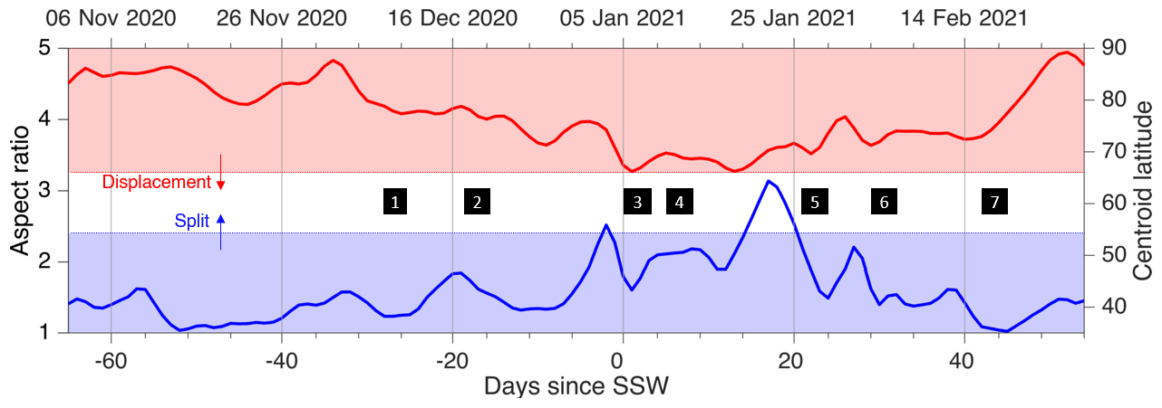
Figure 6 Red line shows the centroid latitude and blue line shows the aspect ratio of the polar vortex around the time of the January 2021 SSW, computed from ERA5 GPH at the 10 hPa level following the method of Seviour et al. (2013). Unshaded region indicates anomalous values indicative of a major vortex distortion, i.e. a split vortex for the blue line or a displaced vortex for the red line. Numbered boxes across the centre of the plot are used to guide discussion from Sect. 6 onwards.

Seviour et al. (2013) empirically defined splits as events where the aspect ratio (blue line) remained ≥2.4 for 7 d or more and displacement events as those where the centroid latitude (red line) dropped equatorward of 66^∘ for more than 7 d. We have here restricted our discussion to the 10 hPa level and note that the geometrical structure of the event may be different in the lower stratosphere, as has been found for previous SSWs (Lawrence and Manney, 2018). Even so, Fig. 9, discussed below, shows some evidence of vortex-splitting taking place at the 82 hPa level.

The January 2021 SSW meets neither the split-event nor the displacement-event criteria of Seviour et al. (2013) at the 10 hPa level but closely approaches both, making it a mixture of the two event types. This is reasonably common, with typically a third of SSWs being neither clear displacements nor splits (Baldwin et al., 2021, and references therein).

The vortex centroid latitude never moves equatorward of 66^∘ but is equatorward of 69^∘ for nine consecutive days from 12 to 20 January. This period falls during the period of most negative zonal winds in the UTLS in our Aeolus data and corresponds temporally to both strongly negative zonal winds at 60^∘ N in MLS $\stackrel{\mathrm{‾}}{u}$ at 32 km (∼10 hPa, Fig. 4b) and in Aeolus $\stackrel{\mathrm{‾}}{u}$ 10 km below this (Fig. 5b).

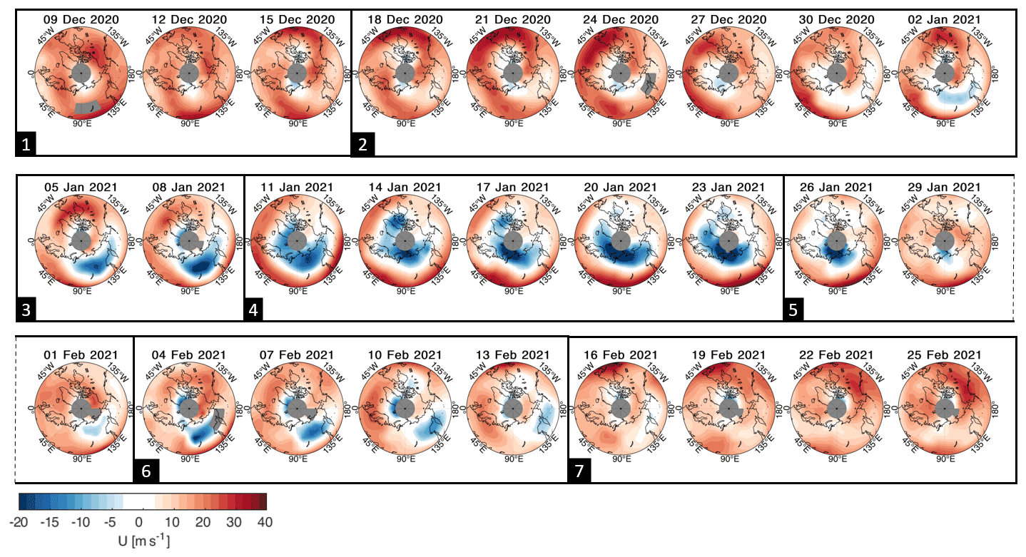
Figure 7 Five-day-mean Aeolus zonal wind at 17 km altitude between 45 and 80^∘ N. Colours show zonal wind speed; note asymmetric colour scale used to better highlight westward winds. Numbered boxes indicate phases of the SSW, defined to help guide discussion in Sect. 6.

The vortex aspect ratio exceeds 2.4 twice, on 3 January for 1 d and starting on 20 January for 6 d, but never meets the 7-consecutive-day element of the Seviour et al. (2013) criteria. Given we are using daily-averaged data for this analysis, it is conceivable that there is a 7 d period offset from the diurnal cycle where the aspect ratio exceeds 2.4, which would allow us to tentatively class this SSW as a split warming; however, such a classification is marginal at best. Under the alternative criteria of Gerber et al. (2021), who first define events by zonal wind reversal and then subdivide into splits and displacements by the number of days in which the thresholds are exceeded within ±10 d of onset, this event would be classified as a split event. The differing results of these two classifications highlight the inherent sensitivity of such threshold-based methods.

6 Vortex structure at sub-zonal scales

Figures 7–9 illustrate the temporal development of Aeolus u and MLS GPH over the course of the SSW.

Figure 8 Three-day-mean Aeolus u between 60^∘ N (indicated by a line at surface level) and 80^∘ N (indicated by the outer surface of the central semi-transparent grey cylinder) for selected dates during winter 2020/21. Values in brackets after each date indicate day numbers relative to 5 January 2021. Outer red (blue) surfaces enclose regions with zonal wind speeds > 15 m s⁻¹ in the eastward (westward) direction; interior red (blue) surfaces enclose regions with wind speeds > 25 m s⁻¹. Terrain is shown at true relative height, using mean values on a 10 km × 10 km regular spatial grid centred at the pole. Isosurfaces have been closed at the limits of the plotted volume for visual clarity but are very likely to extend beyond it in the real atmosphere.

Figure 9 Maps of MLS (a) 10 hPa and (b) 82 hPa GPH in kilometres for selected days. Selected contours have been highlighted in blue and red, with their locations indicated on the colour bars.

Figure 7 shows Aeolus u at 17 km altitude. This altitude level is selected as it is typically the highest altitude level where Aeolus data coverage continues equatorward of 60^∘ N (Fig. 1), allowing the maps to extend further south than this latitude for broader context. The maps show consecutive 5 d means, stepping 3 d between each panel. Three and 1 d means were separately assessed: 1 d means do not provide full geographic coverage, while 3 d means gave broadly the same results but with more noise. For clarity of discussion, we define seven approximate phases of the SSW's life cycle, which are indicated by numbered boxes on the figure. These phases are also labelled on Figs. 5 and 6 for context, with the numbered boxes on these figures indicating the start dates of the phases identified in Fig. 7.

Figure 8 shows 5 d mean Aeolus u for seven dates selected as representative of their phase. The data are plotted inside a volume covering the region poleward of 60^∘ N from heights of 5–22 km and are shown as 3D concentric isosurfaces set at +15 m s⁻¹ (outer red), +25 m s⁻¹ (inner red), −15 m s⁻¹ (outer blue) and −25 m s⁻¹ (inner blue). Surface topography maps shown at the base of each volume are to true vertical scale with the winds, with the 60^∘ N southern data limit indicated by a grey circle at surface level. A semi-transparent grey cylinder fills the region poleward of the northern data limit at 80^∘ N.

Figure 9 shows maps of (upper half) 10 hPa and (lower half) 82 hPa pressure level MLS GPH for the same dates. The 10 hPa level is chosen for consistency with the general literature on SSWs and Fig. 6. The 82 hPa level is chosen as the closest standard MLS pressure level to the 17 km altitude level shown in Fig. 7 (82 hPa ∼17.5 km). Empirically selected contours intended to highlight the shape of the GPH minima are shown in red and blue.

Throughout this section we refer to both the 17 km data in Fig. 7 and the 82 hPa data in Fig. 9 as being at 82 hPa, in order to make clear that we are treating these data as being at the same vertical level, to reduce confusion between kilometres as both a unit of GPH and altitude, and for clarity of prose.

The SSW evolves over our seven phases as follows.

1. Beginnings. In Phase 1, the polar vortex has started to drift off the pole and deform, with an aspect ratio ∼1.3 and centroid latitude of 78^∘ N at 10 hPa (Figs. 6 and 9). At 82 hPa, the vortex-centre GPH minimum is also deformed, with a minimum value at 77^∘ N, 79^∘ E and with noticeable elongations into Europe, Canada and (especially) Central Asia. Zonal winds are strong and positive around this minimum at the 82 hPa level (Fig. 7) except for a local minimum over the Sea of Okhotsk late in the phase. $u>+\mathrm{15}$ m s⁻¹ at all heights within the 60–80^∘ N volume except for this region and the region of minimum GPH itself (Fig. 8). Local u reaches values $u>+\mathrm{30}$ m s⁻¹ over Alaska. While u during this period is atypically strong relative to our climatology (Sect. 3), the observed morphology is similar to that observed by Aeolus earlier in the winter (not shown).

2. Vortex breakdown. In late December and early January, the vortex centroid latitude moves steadily equatorward, with the aspect ratio remaining consistently above 1.4 at both the 10 and 82 hPa levels. As January begins, the vortex elongates along an axis aligned from the Caspian Sea to Hudson Bay, briefly exceeding an aspect ratio of 2.4 at the 10 hPa level (Fig. 6), and multiple independent local minima appear in 82 hPa GPH over northern Canada and over the Arctic Ocean north of Russia and (separately) Scandinavia (Fig. 9). At 82 hPa, we see patches of first white and then blue appearing in Fig. 7, representing localised regions of near-zero and reversing u. The broad GPH minimum's morphology can also be inferred in these Aeolus winds from positive u over mainland Canada and negative u over Russia. Zonal mean $\stackrel{\mathrm{‾}}{u}$ remains positive (Fig. 5), but a significant fraction of the polar volume now has $u<+\mathrm{15}$ m s⁻¹ and small regions reach $u<-\mathrm{15}$ m s⁻¹ at low altitudes (Fig. 8).

3. Onset. The major SSW begins as zonal mean winds at 10 hPa and 60^∘ N reach zero; this occurs around 10 km above the top of our Aeolus measurement volume but can be seen in MLS geostrophic and ECMWF operational and reanalysis winds (Fig. 2). By this time, u has already reversed in a large fraction of the polar UTLS (Fig. 7), spreading outwards from a locus over Siberia which corresponds to a local (but not global) minimum in 82 hPa GPH (Fig. 9). Over the next 2 weeks (i.e. throughout Phases 3 and 4) the vortex remains at its southernmost point and is highly elongated, with a negative GPH anomaly stretching from western Russia and Scandinavia over the North Atlantic and (in the early part of the period) Canada. This period represents the maximum of lower-stratospheric $\stackrel{\mathrm{‾}}{T}$ and the minimum of 60^∘ N $\stackrel{\mathrm{‾}}{u}$ (Figs. 4 and 5), i.e. the peak of the SSW. A volume of positive u>15 m s⁻¹ at high altitudes over North America and low altitudes over northwestern Russia wraps around a volume of negative $u<-\mathrm{15}$ m s⁻¹ at high altitudes over Scandinavia, and at the centre of the region of negative u, zonal wind speeds have reached values as low as $u<-\mathrm{15}$ m s⁻¹ at 82 hPa.

4. Peak SSW. During this phase, the SSW has major effects on winds throughout the lower stratosphere. Near-uniform negative u is seen in all areas poleward of 60^∘ at 82 hPa (Fig. 7), with the exception of a small region over Alaska. This phase corresponds to the negative $\stackrel{\mathrm{‾}}{u}$ patch seen in Fig. 5b at altitudes above 19 km and to the large positive temperature anomaly seen at these heights in Fig. 5a. The spiral wind structure seen in Phase 3 remains, but with the almost complete elimination of regions occupied by $u>+\mathrm{15}$ m s⁻¹ and a large increase in the volume with $u<-\mathrm{15}$ m s⁻¹. During this phase, the zonal wind corresponds approximately in morphology to the form of the GPH vortex, with eastward flows south of the region enclosed by the 18.8 km GPH contour (red line) and westward flows north of the region. This period corresponds to the latter part of the displacement-like period in Fig. 6.

5. Initial recovery. The polar vortex begins to recover in late January. In the latter part of this phase, we see positive u at all locations at 82 hPa except for a small region over the northern Pacific (Fig. 7). This corresponds to the local maximum in $\stackrel{\mathrm{‾}}{u}$ seen in Fig. 5 and represents an initial shift towards a more symmetric vortex morphology. The 10 hPa GPH minimum by this date has shifted eastwards and slightly northwards, becoming more circular and centred over the Arctic ocean poleward of north-central Russia with an extension into eastern Europe. At the 82 hPa level, the GPH minimum is centred slightly southeast of the 10 hPa centre and also forms a single more-circular area covering most of Russia. Winds are strong and zonal along the southern edge of the 82 hPa GPH minimum.

6. Second onset. In Fig. 2, we see a secondary minimum in MLS and reanalysis $\stackrel{\mathrm{‾}}{u}$ at 32 km at the start of this phase. Over the following days, $\stackrel{\mathrm{‾}}{u}$ decreases at all heights (Fig. 5b), and a negative u region at 82 hPa over Russia develops again (Fig. 7), together with a mixture of positive and negative u volumes over Europe and the seas north of Great Britain. A second patch of negative wind also briefly develops over Canada towards the end of this phase in the 82 hPa maps.

7. Final recovery. Finally, the vortex begins to return to a more typical, if still sightly disturbed, state. At both the 10 and 82 hPa levels, the vortex is centred slightly south of, but close to, the pole, with minimum GPH along the 80^∘ W meridian but poleward of 85^∘ N. Winds at 82 hPa are maximal close to, but slight west of, the vortex minimum, with a secondary maximum on the opposite side of the GPH minimum, and follow contours of GPH likely associated with a weak high-mode planetary wave (light purple). By the end of this, phase values of $u>+\mathrm{15}$ m s⁻¹ fill most of the polar volume. This atmospheric state is broadly typical for the zonal mean polar stratosphere at this time of year (Fig. 3), albeit with significant anomaly temperatures at altitudes above our wind data (Fig. 4a).

7 Surface coupling and surface impacts

SSWs often have significant effects on surface weather. These effects typically take place through indirect coupling processes over the weeks following the SSW, including via modulation of the jet stream, the Northern Annular Mode and other processes which imprint upon GPH (e.g. Baldwin and Dunkerton, 2001; Kidston et al., 2015; Ming, 2015; Domeisen et al., 2020).

To investigate such coupling, Fig. 10a shows normalised area-weighted polar-cap-mean GPH anomalies (hereafter Z^′) averaged from 65–90^∘ N derived from ERA5 data relative to a 1979–2020 climatology. ERA5 GPH is used here rather than MLS GPH as above to provide seamless coverage down to the surface and a longer climatological record.

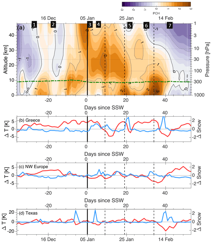
Figure 10 (a) Polar-cap height anomalies (Z^′) around the January 2021 SSW relative to a 1979–2020 climatology, derived from ERA5 GPH. Green dash-dotted line indicates tropopause height. (b–d) Time series of (red, left axis) 2 m temperature anomaly and (blue) fractional snow cover extent for three selected geographic regions. For all panels, the thick solid vertical line indicates the 10 hPa date of the SSW commencing, and the thin dashed lines correspond to local post-SSW minima of Z at zero altitude. Numbered boxes refer to SSW phases discussed above.

We first describe the temporal evolution of Z^′ in the UTLS and above.

• Absolute stratospheric Z^′ does not exceed 1 until the last 2 d of December. Z^′ is negative at the beginning of December, turns positive in mid-December and then becomes negative again until near the end of the month. The positive Z^′ period corresponds to the beginning of the vortex breakdown (Figs. 5, 7 and 9).

• From 26 December, Z^′ increases at all heights. This happens first in the UTLS, where it coincides with falling Aeolus $\stackrel{\mathrm{‾}}{u}$ (Fig. 5). A few days later, Z^′ also begins to increase above 30 km, at the same time as MLS $\stackrel{\mathrm{‾}}{u}$ rapidly reverses (Fig. 4). These separate regions of high Z^′ both spread vertically into the lower stratosphere with time, converging at ∼20 km altitude around the start of the SSW as the vortex centroid reaches its most southerly point and becomes highly elongated (Figs. 6 and 9).

• As the SSW evolves, stratospheric Z^′ remains high for an extended period, with lower-stratospheric $Z^{\prime }>\mathrm{1.75}$ for 20 d and >0 for over 40 d after the SSW commences. In the upper stratosphere, we see $Z^{\prime }>\mathrm{0}$ for most of this period, with a small local maximum at $\sim +\mathrm{25}$ d corresponding to a brief period of increased $\stackrel{\mathrm{‾}}{u}$ in Fig. 5.

• From the beginning of February, Z^′ begins to fall, crossing 0 at the beginning of February at the top of the shown height range and continuing, reaching −1.75 by the end of the month. This decline begins at the highest altitudes before propagating downwards and coincides with zonal wind speeds throughout the column returning to climatology.

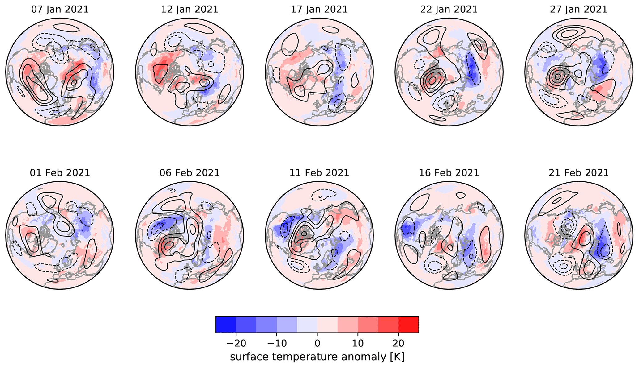
Figure 11 Consecutive 5 d mean maps of ERA5 2 m temperature (shading) and 500 hPa level geopotential height (500GPH, contours) anomalies for the period following the SSW. Values are shown as anomalies from a 1979–2020 climatology for the given dates. The 500GPH contours are at 100 m intervals, negative values are dashed and the zero contour is omitted.

We next investigate how the SSW may have coupled to and affected surface weather, using Z^′ as a proxy metric of stratosphere–troposphere–surface coupling. Z′ is a good proxy for the Northern Annular Mode (NAM) index, which indicates the strength of the polar vortex through the stratosphere. In some regions the surface impacts of cold air outbreaks are approximately proportional to the anomalous strength of the polar vortex in the lower stratosphere (Baldwin and Dunkerton, 2001; Baldwin et al., 2021); however, in other regions, for example North America, vortex morphology may be more related to surface impacts (Lee et al., 2019).

To quantify surface weather effects, Fig. 11 shows maps of consecutive 5 d mean 2 m temperature anomalies (hereafter 2mT^′) and 500 hPa level geopotential height (hereafter “500GPH”) anomalies at the hemispheric scale from the beginning of the SSW to the end of February. Supporting our discussion, we also (Fig. 10b–d) show snow cover anomalies and 2mT^′ averaged over Greece (20–30^∘ E, 35–45^∘ N), northwestern Europe (10^∘ W–20^∘ E, 45–65^∘ N) and Texas (105–95^∘ W, 25–35^∘ N). The 2mT^′ and the snowfall anomalies have been derived from ERA5 output. Figures 10 and 11 are again computed relative to a 1979–2020 climatology.

We structure our discussion in terms of Fig. 11, referring to Fig. 10b–d to highlight some selected specific events with a strong possibility of stratospheric linkages.

From 7 January, we see negative 2mT^′ over western Europe, associated with the heaviest snowfall in Spain for over 50 years. Based on both the early date of this event relative to the SSW life cycle and on the lack of any obvious Z^′ feature linking the stratospheric vortex breakdown to the surface (Fig. 10a), we believe that this event was not caused by the SSW. The lower average temperatures in Europe prior to and around the commencement of the SSW are, however, consistent with previous work linking SSWs to cold air outbreaks (e.g. Kolstad et al., 2010; King et al., 2019, and references therein). There are notable regions of positive 2mT^′' over Siberia and the Arctic Ocean, as well as North America, which weaken and strengthen respectively by 12 January and are congruent with positive 500GPH anomalies.

By 17 January, 2mT^′ surface structures characteristic of SSW surface impacts have begun to appear (e.g. Butler et al., 2017; Lee et al., 2019; Kretschmer et al., 2018), with a cold anomaly in Siberia and a warm anomaly over Baffin Bay, associated with positive and negative 500GPH anomalies respectively. This follows the development of a positive Z^′ link from the lower stratosphere to the surface (first dotted line from left, Fig. 10). Over the days following this Z^′ link, we also see reduced 2mT^′ and anomalously heavy snowfall over Greece (Fig. 10b), together with a local maximum in snow and minimum in 2mT^′ over NW Europe (Fig. 10c). A negative North Atlantic Oscillation (NAO)-like pattern is evident over the Atlantic from 22 January, although the centres of action shift during the subsequent weeks. This is indicative of a southward shift in the North Atlantic polar front jet stream and storm track, which are associated with cold air outbreaks over Europe (e.g. Kidston et al., 2015; Domeisen et al., 2020)

From 27 January, negative 2mT^′ begins to appear over the mainland United States and positive 2mT^′ in the Middle East, simultaneously with a low-altitude maximum of $Z^{\prime }>\mathrm{2}$ (Fig. 10a), both of which are components of the typical SSW surface signal in 2mT^′ (Butler et al., 2017). An unusual feature here is the development of positive 2mT^′ over the Urals, which persists into early February and is associated with high pressure over the Urals advecting warm air from the south. This feature may have acted to inhibit westward extension of Siberian cold anomalies and prevented northeastern Europe from developing a strong cold anomaly before this date.

From 1 February, low 2mT^′ moves southward over North America, starting over Alaska and western Canada, then intensifying over the mainland United States, and reaching Texas by 11 February. This US cold air outbreak was the coldest February weather in this region since 1989 and can be clearly seen in Fig. 10d as a very large negative 2mT^′ ($\sim -\mathrm{20}$ K relative to climatology) with a number of days of high snowfall anomalies which commence synchronously with a strong positive $Z^{\prime }>\mathrm{3}$ and in turn suggests a strong possibility of a role for stratosphere–troposphere coupling. The cold outbreak was intensified by increased high pressure over the Aleutian region which acted to block the jet stream, associated with a southward loop of the jet downstream of the block and advecting cold air southwards (Fig. 11; see e.g. Kodera et al., 2013). The increased Aleutian high here may have been in part due to pre-existing La Niña conditions in the tropical Pacific during this winter; furthermore, increased blocking, seen in the 500GPH anomalies for 1–11 February (Fig. 11) over the Canadian Archipelago, may have acted to push cold further south than usual.

Northwestern Europe experiences its most intense cold spell from 1 to 11 February, also synchronously with this large Z^′ anomaly. A local-minimum temperature was reached at Braemar on 11 February, which at 250 K was the lowest UK temperature since 1995. These cold anomalies shift eastwards by 16 February, explaining the delay in the development of cold snowy weather in Greece relative to NW Europe and leading to Athens experiencing 20–25 cm of snow on 15 and 16 February.

Although data of this type cannot show a direct causal link, our data strongly suggest that the early January SSW may have acted as either a trigger or an intensifier for several extreme winter weather events affecting densely populated regions of the Northern Hemisphere over the next 2 months. Even if the SSW did play an important role in these extreme events, our analysis is also not able to explain why different regions may have been impacted at different times during the SSW evolution; such an investigation is left to future studies. Other studies suggest that North America and Eurasia are influenced in different ways by variations in weakening of the stratospheric polar vortex, such as differences in vortex morphology (e.g. Kretschmer et al., 2018; Lee et al., 2019).

8 Summary and conclusions

In this study, we have used Aeolus Rayleigh-clear wind data; MLS temperature and GPH data; and ERA5 temperature, wind, GPH and snowfall output to study the evolution of the early-2021 Northern Hemisphere sudden stratospheric warming event.

Under the empirical criteria of Seviour et al. (2013) which we apply here, this SSW was a mixture of split and displacement types, with the vortex displaced long enough but not far enough south to be a displacement event, and with an aspect ratio elliptical enough but for too brief a period to be a split event. Zonal mean temperature and wind anomalies were broadly within the climatological range of other 21st-century SSW events (Sect. 3): while date-maximum temperatures and date-minimum zonal winds were seen during the event relative to a 2004–2020 climatology, these values were broadly consistent with the anomalies seen during other 21st century SSWs with different commencement dates.

This study represents the first use of Aeolus data to study an SSW, and one of the first scientific uses of this unique dataset, the first systematic measurements of global-scale winds in the free troposphere and lower stratosphere. We demonstrate that Aeolus Rayleigh data are suitable for studying many aspects of dynamically extreme events such as SSWs: Aeolus-observed winds agree well with those inferred from MLS GPH and simulated by ERA5 (Sect. 2.4), and the high spatial resolution of the product allows us to produce maps showing detailed and internally consistent 2D and 3D zonal wind structure (Sect. 6). These maps also show excellent agreement at a physical level with the evolution of the vortex in MLS GPH (Sect. 6).

The Aeolus data also clearly exhibit relatively fine vertical structures, including a pole-wrapping zonal wind feature seen in Fig. 8 during the peak of the SSW, which is only a few kilometres in vertical extent at any given height and remains visible in the data even after applying heavy vertical (2 km), horizontal ($\mathrm{5}{}^{\circ }\times \mathrm{20}{}^{\circ }$) and temporal (5 d) averaging to ensure full coverage. Although we do not do so here, exploitation of Aeolus Rayleigh data at its true spatiotemporal resolution and of the even finer-resolution Mie data could provide additional useful information on possible filamentary wind structures related to the vortex breakdown before and during the SSW.

Finally, study of ERA5 GPH and snowfall output in the context of the SSW (Sect. 7) suggests that this SSW coupled downwards to the surface and supports the hypothesis that several major extreme-weather events during January and February 2021, including cold and snow cover extent extrema in Greece, northwestern Europe and, especially, Texas, were likely related to some degree to the SSW at the beginning of the year. This demonstrates the large and significant impact of SSWs on surface climate and highlights the importance of improving our stratospheric forecasting capabilities.

Appendix A: Deriving estimated zonal and meridional winds from Aeolus HLOS wind measurements

The horizontal line-of-sight (HLOS) wind measured by Aeolus is a projection of the horizontal zonal and meridional wind vectors u and v into a single along-line-of-sight direction. The measured HLOS wind u_HLOS is the sum of the two components

$$\begin{array}{}\text{(A1)}& u_{\mathrm{HLOS}}=-(\mathit{u}\sin \mathit{\theta }+\mathit{v}\cos \mathit{\theta }),\end{array}$$

where θ is defined as the reflex angle measured from north to the direction along the line of sight of the ALADIN instrument. Because the lidar points at a 90^∘ angle to the direction of travel, this results in a different projection during ascending (“asc”) and descending (“desc”) nodes of the orbit, specifically

$$\begin{array}{}\text{(A2)}& {\displaystyle }& {\displaystyle }-u_{\mathrm{HLOS},\mathrm{asc}}=\mathit{u}\sin \left(\mathit{\theta }\right)+\mathit{v}\cos \left(\mathit{\theta }\right),\text{(A3)}& {\displaystyle }& {\displaystyle }-u_{\mathrm{HLOS},\mathrm{desc}}=\mathit{u}\sin (-\mathit{\theta })+\mathit{v}\cos (-\mathit{\theta }).\end{array}$$

If we define a latitude–longitude–height–time box, we can estimate the true (i.e. unprojected) average horizontal zonal and meridional wind vectors $\stackrel{\mathrm{‾}}{\mathit{u}}$ and $\stackrel{\mathrm{‾}}{\mathit{v}}$ for this box by averaging all HLOS wind measurements that fall within the box for both ascending and descending orbits. This uses the different information content of the two scanning directions to cancel out directional uncertainties in measurement. For the average meridional wind vector $\stackrel{\mathrm{‾}}{\mathit{v}}$, we compute this as

$$\begin{array}{}\text{(A4)}& \begin{array}{rl}\stackrel{\mathrm{‾}}{\mathit{v}}& =\left(u_{\mathrm{HLOS},\mathrm{asc}}+u_{\mathrm{HLOS},\mathrm{desc}}\right)/\mathrm{2}\cos \mathit{\theta }\\ & =(\mathit{u}\sin \mathit{\theta }+\mathit{v}\cos \mathit{\theta }+\mathit{u}\sin (-\mathit{\theta })+\mathit{v}\cos (-\mathit{\theta }\left)\right)/\mathrm{2}\cos \mathit{\theta }\\ & =\left(\mathrm{2}\mathit{v}\cos \mathit{\theta }\right)/\mathrm{2}\cos \mathit{\theta }\\ & =\mathit{v}\end{array}\end{array}$$

and for zonal wind $\stackrel{\mathrm{‾}}{\mathit{u}}$ as

$$\begin{array}{}\text{(A5)}& \begin{array}{rl}\stackrel{\mathrm{‾}}{\mathit{u}}& =\left(u_{\mathrm{HLOS},\mathrm{asc}}-u_{\mathrm{HLOS},\mathrm{desc}}\right)/\mathrm{2}\sin \mathit{\theta }\\ & =(\mathit{u}\sin \mathit{\theta }+\mathit{v}\cos \mathit{\theta }-\mathit{u}\sin (-\mathit{\theta })-\mathit{v}\cos (-\mathit{\theta }\left)\right)/\mathrm{2}\sin \mathit{\theta }\\ & =\left(\mathrm{2}\mathit{u}\sin \mathit{\theta }\right)/\mathrm{2}\sin \mathit{\theta }\\ & =\mathit{u}.\end{array}\end{array}$$

We use this method to estimate u for all Aeolus measurements presented in this study, with our boxes defined to each cover a region of 2.5×22.5^∘ in latitude and longitude respectively and 2 km in height – this box size is chosen to give full geographic coverage at a daily level. To improve vertical resolution at a small cost of point-to-point independence, we step the boxes in height at intervals of 1 km. To compute zonal mean winds, we apply the same method, but using a 360^∘ box width in longitude.

For most figures shown in this study, we use boxes with a width of 1 d in time, except in Sect. 6 where we use sliding 5 d fits as described there. These temporally wider boxes have reduced point-to-point noise and hence allow relatively detailed spatial mapping but at a cost of day-to-day independence.

A fundamental assumption of this method is that any given ascending scan samples broadly the same wind field over a given region as the subsequent descending scan (or vice versa). This assumption can be broken down into three distinct error sources: (1) the heterogeneity of the background wind over the spatiotemporal extent of the box; (2) the spatial separation between ascending and descending scans within that box, which varies with latitude and can be as much as 2000 km in the tropics; and (3) the separation in time between ascending and descending scans, which can be as much as 12 h in local time. This means that longitudinal gradients in wind speed at scales of hundreds of kilometres, or significant changes in wind speed over timescales of less than 12 h, will introduce errors in the winds computed using this method, as the above assumptions can become invalid. At high latitudes, such as those presented here, the spatiotemporal separation between measurements is relatively low, and thus these three sources of error are all minimised but will be larger at lower latitudes. In particular, we do not expect systematic differences between measurements during daytime and nighttime since the effects of atmospheric tides are weak at the altitudes considered here, significantly ameliorating (3).

Our results as presented are relatively insensitive to the precise details of this method. For example, a preprint version of this study (available via the journal web page for this article) used simple estimates of u projected directly from individual HLOS measurements, rather than these more complicated profile-matching approaches, but produced very similar results for all figures presented except for a slight reduction in measured absolute wind speeds, which this method corrects for.