The importance of horizontal model resolution on simulated precipitation in Europe – from global to regional models

Precipitation is a key climate variable that affects large parts of society, especially in situations with excess amounts. Climate change projections show an intensified hydrological cycle through changes in intensity, frequency, and duration of precipitation events. Still, due to the complexity of precipitation processes and their large variability in time and space, climate models struggle to represent precipitation accurately. This study investigates the simulated precipitation in Europe in available climate model ensembles that cover a range of horizontal model resolutions. The ensembles used are global climate models (GCMs) from CMIP5 and CMIP6 (∼100–300 km horizontal grid spacing at mid-latitudes), GCMs from the PRIMAVERA project at sparse (∼80–160 km) and dense (∼25–50 km) grid spacing, and CORDEX regional climate models (RCMs) at sparse (∼50 km) and dense (∼12.5 km) grid spacing. The aim is to seasonally and regionally over Europe investigate the differences between models and model ensembles in the representation of the precipitation distribution in its entirety and through analysis of selected standard precipitation indices. In addition, the model ensemble performances are compared to gridded observations from E-OBS.

The impact of model resolution on simulated precipitation is evident. Overall, in all seasons and regions the largest differences between resolutions are seen for moderate and high precipitation rates, where the largest precipitation rates are seen in the RCMs with the highest resolution (i.e. CORDEX 12.5 km) and the smallest rates in the CMIP GCMs. However, when compared to E-OBS, the high-resolution models most often overestimate high-intensity precipitation amounts, especially the CORDEX 12.5 km resolution models. An additional comparison to a regional data set of high quality lends, on the other hand, more confidence to the high-resolution model results. The effect of resolution is larger for precipitation indices describing heavy precipitation (e.g. maximum 1 d precipitation) than for indices describing the large-scale atmospheric circulation (e.g. the number of precipitation days), especially in regions with complex topography and in summer when precipitation is predominantly caused by convective processes. Importantly, the systematic differences between low resolution and high resolution also remain when all data are regridded to common grids of $\mathrm{0.5}{}^{\circ }\times \mathrm{0.5}{}^{\circ }$ and $\mathrm{2}{}^{\circ }\times \mathrm{2}{}^{\circ }$ prior to analysis. This shows that the differences are effects of model physics and better resolved surface properties and not due to the different grids on which the analysis is performed. PRIMAVERA high resolution and CORDEX low resolution give similar results as they are of similar resolution.

Within the PRIMAVERA and CORDEX ensembles, there are clear differences between the low- and high-resolution simulations. Once reaching ∼50 km the difference between different models is often larger than between the low- and high-resolution versions of the same model. For indices describing precipitation days and heavy precipitation, the difference between two models can be twice as large as the difference between two resolutions, in both the PRIMAVERA and CORDEX ensembles. Even though increasing resolution improves the simulated precipitation in comparison to observations, the inter-model variability is still large, particularly in summer when smaller-scale processes and interactions are more prevalent and model formulations (such as convective parameterisations) become more important.

1 Introduction

Precipitation is a key climate variable affecting the environment and human society in different ways and on several temporal and spatial scales. In particular, heavy-precipitation events may lead to large damages caused by floods or landslides, while the absence of precipitation may cause droughts and has an impact on water and hydropower supply. In recent decades there has therefore been extensive study, and considerable advancement in our understanding, of the response of extreme precipitation to climate change (O'Gorman, 2012; Kharin et al. 2013; Donat et al., 2016; Pfahl et al., 2017). For example, it is widely held through theoretical considerations and model experiments that extremes will respond differently than changes in mean precipitation (e.g. Allen and Ingram, 2002; Pall et al., 2007; Ban et al., 2015).

Still, the simulation of precipitation in weather and climate models is challenging because of the wide range of processes involved that act and interact on widely different temporal and spatial scales. An accurate representation of precipitation in models requires skill in simulating (1) the large-scale circulation, (2) interaction of the flow with the surface, and (3) convection and cloud processes. With the typical horizontal grid resolution of O (100 km) of global climate models (GCMs) point (1) can to a large extent be properly represented but less so for (2) and (3) (e.g. van Haren et al., 2015; Champion et al., 2011; Zappa et al., 2013). In particular, atmospheric convective processes are not resolved and need to be treated with convection parameterisations. As the range of scales resolved is broadened through refining the horizontal grid spacing, the simulation of precipitation generally improves. This is achieved through more realistic representation of surface characteristics (such as topography, coastlines, and inland lakes and water bodies) and through more accurately solving the motion equations, resulting in more accurate horizontal moisture transport and moisture convergence (Giorgi and Marinucci, 1996; Gao et al., 2006; Prein et al., 2013a). Indeed, GCMs with ∼25–50 km grid spacing show promise to improve simulation of precipitation (van Haren et al., 2015; Delworth et al., 2012; Kinter et al., 2013; Haarsma et al., 2016; M. J. Roberts et al., 2018; Baker et al., 2019).

Dynamical down-scaling of GCMs with regional climate models (RCMs) allows for even finer grids, which leads to more detailed information of and further improvements in regional and local climate features, for example spatial patterns and distributions of precipitation in areas of complex terrain (Rauscher et al., 2010; Di Luca et al., 2011; Prein et al., 2013b). This can also have important implications for climate change signals. Giorgi et al. (2016) found that an ensemble of RCMs at ∼12 km grid spacing consistently showed an increase in summer precipitation over the Alps region, which contrasted the forcing GCMs that instead showed a decrease. The different responses were attributed to increased convective rainfall in the RCMs due to enhanced potential instability by surface heating and moistening at high altitudes not captured by the GCMs. Differences in the treatment of aerosols are also identified as a reason for differences in climate response between RCMs and GCMs (Boé et al., 2020; Gutiérrez et al., 2020). RCMs are constrained by the lateral boundary conditions provided by the forcing GCM, and studies of RCM ensembles have shown that the choice of forcing GCM has introduced the major part of the overall uncertainty in regional climate (e.g. Déqué et al., 2007; Kjellström et al., 2011). This effect is relatively more important for large-scale precipitation systems, for example frontal systems associated with extra-tropical cyclones. In seasons and regions when smaller-scale processes like convection dominate, for example in summer over mid-latitudes, simulated precipitation is to a larger degree dependent on the RCM itself, in terms of grid resolution and sub-grid-scale parameterisations (e.g. Iorio et al., 2004). A recent study investigated the effects of model resolution on local precipitation on short timescales and found that the 12.5 km simulations better represent daily and sub-daily extreme and mean precipitation, also when simulations are aggregated to 50 km (Prein et al., 2016). They note, however, that the results are highly dependent on which observations the simulations are compared with and that improvements are seen for the ensemble mean, and not necessarily for each individual model. In studies similar to the present one, Iles et al. (2020) and Demory et al. (2020) compare simulations from the CORDEX, CMIP5, and PRIMAVERA ensembles. The results show increases in precipitation with resolution and, when compared to a mixture of E-OBS and high-spatial-resolution gridded national data sets, CMIP5 underestimates precipitation amounts while CORDEX overestimates them, the effect of grid resolution being largest in areas with complex topography. They also find that PRIMAVERA performs similarly to CORDEX when run on the same resolution, which is interesting regarding that the PRIMAVERA models are developed for low resolutions. Iles et al. (2020) concluded from the considerable inter-model differences that improvements are seen for the ensemble mean rather than for individual models.

Although increased grid resolution often leads to improved simulation of precipitation, convection is usually not resolved by the model dynamics, even at grid spacings of around 10 km but is instead parameterised (although it might be possible to turn off the parameterisation already at this kind of resolution; Vergara-Temprado et al., 2019). The choice of convection parameterisation can have various effects on the occurrence and amount as well as on the onset timing and location (e.g. Dai et al., 1999; Dai, 2006; Stratton and Stirling, 2012; Gao et al., 2017). Commonly, models with parameterised convection exhibit biases in the diurnal precipitation cycle (Liang, 2004; Brockhaus et al., 2008; Gao et al., 2017), sometimes regardless of increases in grid resolution (Dirmeyer et al., 2012). In addition, models of coarse resolution often suffer from simulating precipitation over too large of an area compared to observations and usually also too many days with weak precipitation (the “drizzle” problem) (e.g. Dai, 2006; Stephens et al., 2010). At sufficiently high resolution (<4 km), models start to largely resolve deep convection, enabling the parameterisation to be turned off, so called “convection-permitting” models (Prein et al., 2015; Vergada-Temprado et al., 2019). Convection-permitting regional climate models (CPRCMs) are widely shown to reduce, at least to some extent, these biases, most evidently by improving the match of the diurnal cycle to observations (e.g. Prein et al., 2013a; Ban et al., 2014; Brisson et al., 2016; Gao et al., 2017; Leutwyler et al., 2017; Belušić et al., 2020) and better representation of sub-daily high-intensity precipitation events (e.g. Ban et al., 2014; Kendon et al., 2014; Fosser et al., 2015; Lind et al., 2020) than models with parameterised convection. A major draw-back using these high-resolution climate models is the very high computational cost, causing their use in ensembles to only recently emerge (Coppola et al., 2018).

The aim of this study is to

• i.

  investigate to what extent a large number of global and regional climate models can reproduce observed daily precipitation climatologies and characteristics over Europe, and

• ii.

  investigate how horizontal model grid resolution in either global or regional models affects the simulated precipitation in Europe: are there systematic differences? If so, are these persistent for different parts of Europe and for different seasons?

To this end, GCMs of standard resolution from CMIP5 (Climate Model Intercomparison Project Phase 5; Taylor et al., 2012) are compared with GCMs which participated in the HighResMIP (High Resolution Model Intercomparison Project; Haarsma et al., 2016) experiment within the H2020 EU project PRIMAVERA. These models are ECMWF-IFS (C. D. Roberts et al., 2018), HadGEM3-GC31 (Roberts et al., 2019), MPI-ESM1.2 (Gutjahr et al., 2019), CNRM-CM6.1 (Voldoire et al., 2019), and EC-Earth3P (Haarsma et al., 2020). Furthermore, the first results from the CMIP6 (Climate Model Intercomparison Project Phase 6; Eyring et al., 2016) GCMs are included in the analysis. The GCMs are compared with RCMs from CORDEX (Coordinated Regional Downscaling Experiment; Gutowski et al., 2016). This allows for comparisons of different generations of models, global versus regional models, and the impact of horizontal model grid resolutions. For a few cases, the same model version has been applied at two different grid resolutions, which allows for investigating the impact of resolution alone. The simulated daily precipitation is analysed in terms of both precipitation intensity distributions and a collection of standard precipitation-based indices.

2 Models and methods

2.1 Global and regional models

The models used in this study are a selection of CMIP5 global models (corresponding to ∼100–300 km horizontal grid spacing at mid-latitudes); the high-resolution (∼25–50 km) and low-resolution (∼80–160 km) versions of the PRIMAVERA global models and the first available runs from CMIP6 (∼100–300 km); and finally, a selection of CORDEX RCMs (at 12.5 and 50 km mid-latitude grid spacing). The low-resolution versions in each model ensemble are called LR, and the high-resolution HR. Note that not the full CMIP5, CMIP6, and CORDEX ensembles are used, but rather “ensembles of opportunity” for which daily precipitation were readily available. Table 1 lists the GCM ensembles used. Table 2 lists the GCM RCM combinations used in the CORDEX ensembles. The simulated precipitation for all models is analysed over the PRUDENCE regions in Europe (Fig. 1; Christensen and Christensen, 2007). Prior to analysis all grid points over sea are filtered out, and then for each region and model we calculate precipitation characteristics for all remaining land grid points. The simulations are analysed on their native grids, because this is the kind of data that users of climate simulations will face, and since all interpolation may alter precipitation characteristics (Klingaman et al., 2017). Nevertheless, to investigate all aspects of changed resolution, it is sometimes necessary to compare simulations on a common grid. In these cases, the results are also aggregated to two common grids with $\mathrm{2}{}^{\circ }\times \mathrm{2}{}^{\circ }$ and $\mathrm{0.5}{}^{\circ }\times \mathrm{0.5}{}^{\circ }$ grid spacing respectively.

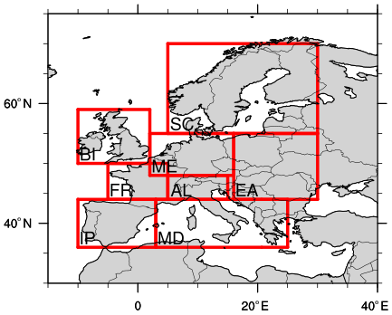
Figure 1 The regions for which precipitation data are analysed: Scandinavia (SC), British Isles (BI), mid-Europe (ME), France (FR), the Alps (AL), eastern Europe (EA), Iberian Peninsula (IP), and the Mediterranean (MD).

Table 1 The GCM ensembles used in this study and the GCMs they consist of. Grid spacing is given in the same format as in the meta-data for each model.

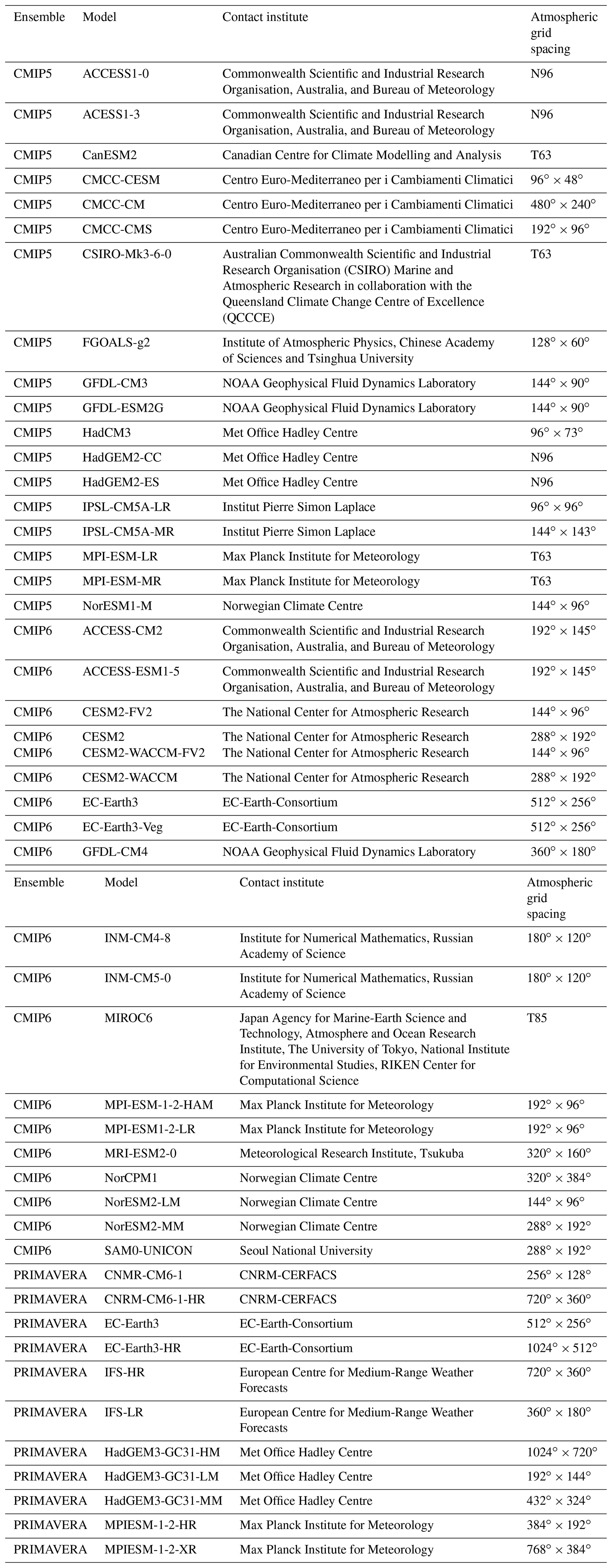
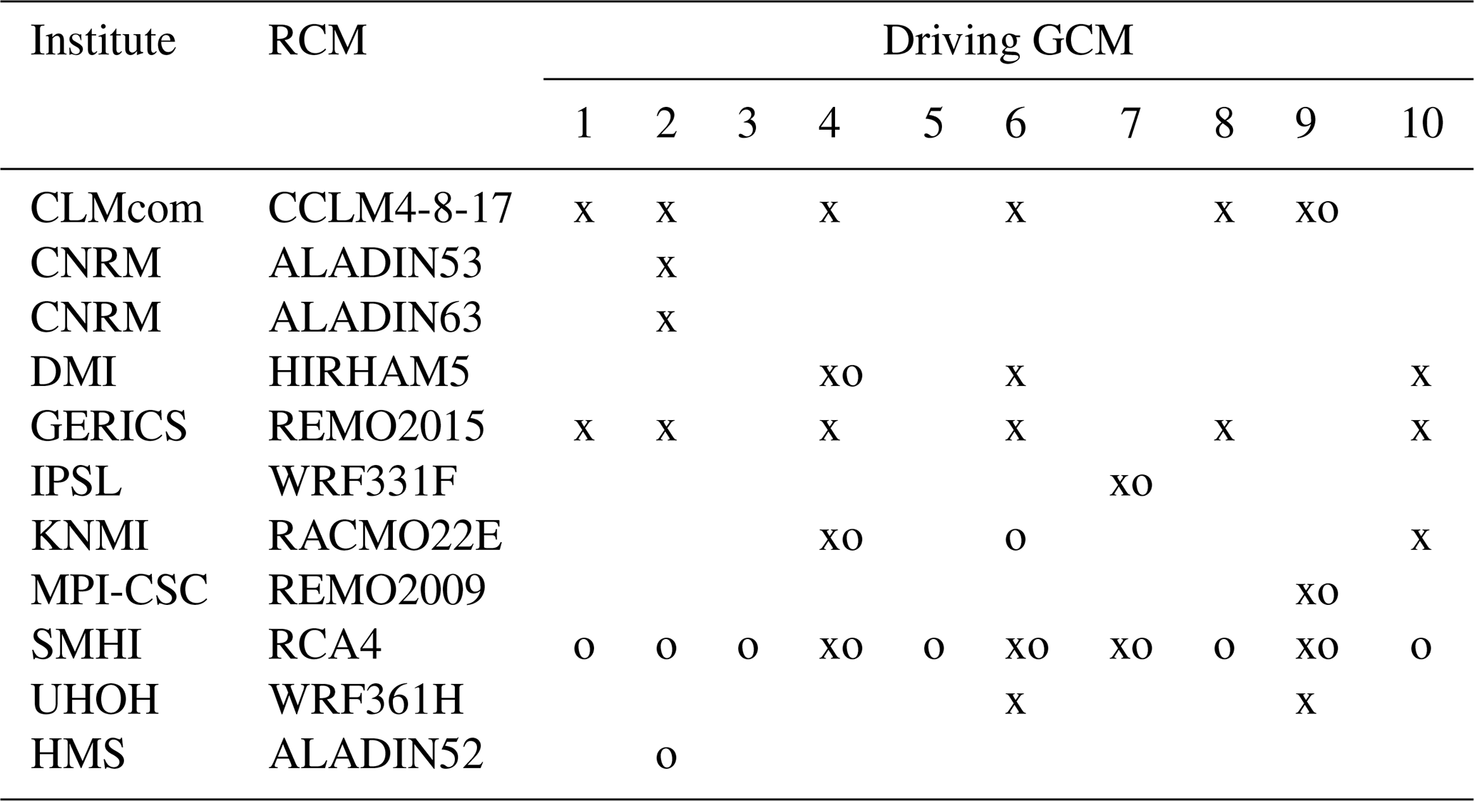
Table 2 RCM GCM combinations used in this study. EURO-CORDEX simulations at 0.11^∘ (∼12.5 km) are marked with “x” and at 0.44^∘ (∼50 km) are marked with “o”. The driving GCMs are (1) CanESM2, (2) CNRM-CM5, (3) CSIRO-Mk3-6-0, (4) EC-Earth, (5) GFDL-ESM2M, (6) HadGEM2-ES, (7) IPSL-CM5A-MR, (8) MIROC5, (9) MPI-ESM-LR, and (10) NorESM1-M.

2.2 Observations

Climate model evaluation exercises often rely, when possible, on gridded reference data sets. In this study daily precipitation sums in models are compared with data from E-OBS version 19.0e at 0.1 and 0.25^∘ grid spacing (Cornes et al., 2018). E-OBS comprises daily station values interpolated onto a grid that spans the entire European continent. The main advantage of using E-OBS is the large geographical coverage at a relatively high resolution available over an extended (climatological) time period. It enables a consistent model–observation comparison over the whole continental part of Europe, with its varying climatological and environmental characteristics.

Gridded products, such as E-OBS, involve spatial analysis and interpolation of point measurements onto a regular grid and are inherently associated with uncertainties originating from both non-climatic influences (e.g. inaccuracies in measurement devices or relocation of measurement sites) and from sampling issues associated with weather and environmental conditions, for example in situations with snowfall in windy conditions (Kotlarski et al., 2019; Rasmussen et al., 2012). The quality of such data sets largely depends on the availability of stations to base the interpolation on, implying that in regions where station density is low the quality of the gridded product is also lower (Herrera et al., 2019). For precipitation this is of even greater importance due to its highly heterogeneous character in both time and space, in particular for high-intensity precipitation events (extremes). These are often local in character (temporally and spatially), even in cases when embedded in larger-scale (synoptic) precipitation systems and can thus be heavily undersampled (Herrera et al., 2019; Prein and Gobiet, 2017). Furthermore, mountainous areas act as strong forcing of precipitation giving rise to large spatial variability over the terrain. The lack of dense networks of stations in these regions combined with a higher occurrence of snowfall makes it very difficult to achieve highly reliable data over mountains (e.g. Hughes et al., 2020; Lundquist et al., 2019).

The quality of E-OBS varies over Europe (see Fig. 1 in Cornes et al., 2018); the station density is for example very high over Scandinavia, Germany, and Poland, while it is lower in eastern Europe and in the Mediterranean region. Gridded regional or national data sets may offer higher quality as these are generally based on a denser station network and are often also provided with higher spatial and/or temporal resolution compared to E-OBS (Kotlarski et al., 2019, Prein and Gobiet, 2017). Here, we limit the comparison to E-OBS only. However, to assess the impact of high-quality regional data, an additional analysis of the precipitation distributions was performed, using ASoP (analysing scales of precipitation) analysis (see Sect. 2.3), comparing models and E-OBS against the NGCD (Nordic Gridded Climate Dataset; Lussana et al., 2018) data set. NGCD is based on daily station data for precipitation and temperature, interpolated onto a 1 km × 1 km grid covering Scandinavia.

2.3 ASoP and precipitation indices

To investigate the effect of model grid resolution on the full distributions of daily precipitation intensities, we use the ASoP method (Klingaman et al., 2017; Berthou et al., 2018). ASoP involves splitting precipitation distributions into bins of different intensities and then provides information of the contributions from each precipitation intensity separately to the total mean precipitation rate (i.e. given by all intensities taken together). In the first step, precipitation intensities are binned in such a way that each bin contains a similar number of events, with the exception of the most intense events, which are rare. The actual contribution (in millimetres) of each bin to the total mean precipitation rate is obtained by multiplying the frequency of events by the mean precipitation rate. The sum of the actual contributions from all bins gives the total mean precipitation rate. The fractional contribution (in percent) of each bin is further obtained by dividing the actual contributions by the mean precipitation rate. In this case, the sum of all fractional contributions is equal to 1; thus the information provided by fractional contributions is predominantly about the shape of the distribution. Taking the absolute differences between two fractional distributions and sum over all bins gives a measure of the difference in the shapes of the precipitation distributions. This is here called the “index of fractional contributions”. Since E-OBS precipitation intensities, in contrast to model data, are not continuous, the resulting ASoP factors for E-OBS tend to be noisy, especially for lower intensities. In order to facilitate the interpretation of the results, the regionally averaged ASoP factors for E-OBS were smoothed to some extent by using a simple filter.

Table 3 Definitions of indices.

The ASoP method is here applied to grid points pooled over target regions (Fig. 1) separately, and the result is a distribution for each model showing the probability of different precipitation intensities based on daily precipitation. Most results presented here concern the actual contributions, both to limit the number of figures and because these factors conveniently provide information on both shape of distributions and the mean values. The ASoP distributions of all analysed models are used to compare model behaviour and performance, in particular to see how changing the grid resolution affects different parts of the distribution, for example if contributions from low and high precipitation intensities are different.

In addition to ASoP, a number of indices based on daily precipitation (listed in Table 3) are calculated for the same regions. For each model, the indices are calculated separately for each grid point within a region (land points only), and the values are then pooled to calculate percentiles representing the region. This also means that the calculated model spread reflects geographical and not temporal variability. The index percentiles are represented by box plots (Sect. 3).

3 Results

3.1 ASoP analysis

3.1.1 Annual precipitation

Since the ASoP results are very similar between CMIP5 and CMIP6 GCMs (not shown), the results presented here include only one of these ensembles, CMIP6. Figure 2 presents the actual contributions (normalised bin frequency times mean bin rate) for annual daily precipitation over four of the PRUDENCE regions: Scandinavia, mid-Europe, the Alps, and the Mediterranean. In general, the model ensembles have higher amounts of precipitation compared to E-OBS, signified by larger contributions at low (<2–3 mm d⁻¹) and moderate to high (>5–10 mm d⁻¹) intensities. An exception is the CMIP6 ensemble that instead shows lower contributions for moderate to high precipitation intensities, i.e. above 10–20 mm d⁻¹ (Scandinavia, mid-Europe, and the Alps) or between 5–20 mm d⁻¹ (Mediterranean). CMIP6 also tends to have the largest overestimates of contributions from the lower intensities (below 5 mm d⁻¹). Another consistent feature is that the probabilities for the higher intensities (above 15 mm d⁻¹) increase with increasing grid resolutions of respective model ensemble, and consequently the contributions become increasingly larger than E-OBS (Fig. 2). This is most evident for the Alps region where the CMIP6 models (100–300 km grid spacing) clearly give smaller contributions than E-OBS and the PRIMAVERA models (25–160 km), the latter having smaller contributions than the CORDEX LR models (50 km) and the CORDEX HR models (12.5 km). The higher-resolution models peak at higher intensities and have wider distributions with larger contributions from high-intensity daily rates. The sensitivity of model grid resolution to precipitation amounts and variability in association with areas with complex and steep topography (e.g. Prein et al., 2015) is most likely the main reason for the large differences between model ensembles in the Alps region. For example, the upper end of the CMIP6 distributions is around 50 mm d⁻¹ while the corresponding part in CORDEX HR models is around 100 mm d⁻¹ (bottom right panel in Fig. 2). To further verify the results, the same analysis was performed after all data had been interpolated (conservatively) to two common grids: one at 2${}^{\circ }\times \mathrm{2}{}^{\circ }$ resolution and one at $\mathrm{0.5}{}^{\circ }\times \mathrm{0.5}{}^{\circ }$ resolution (Figs. S1 and S2 in the Supplement). The interpolation to either grid has an overall small impact on the results. With the coarser grid ($\mathrm{2}{}^{\circ }\times \mathrm{2}{}^{\circ }$) the ASoP actual contributions have relatively larger contributions from the bulk part and a smaller contribution from the highest intensities, as expected from the smoothing effect of interpolation. These results provide increased confidence in the conclusions drawn from analysis on native grids.

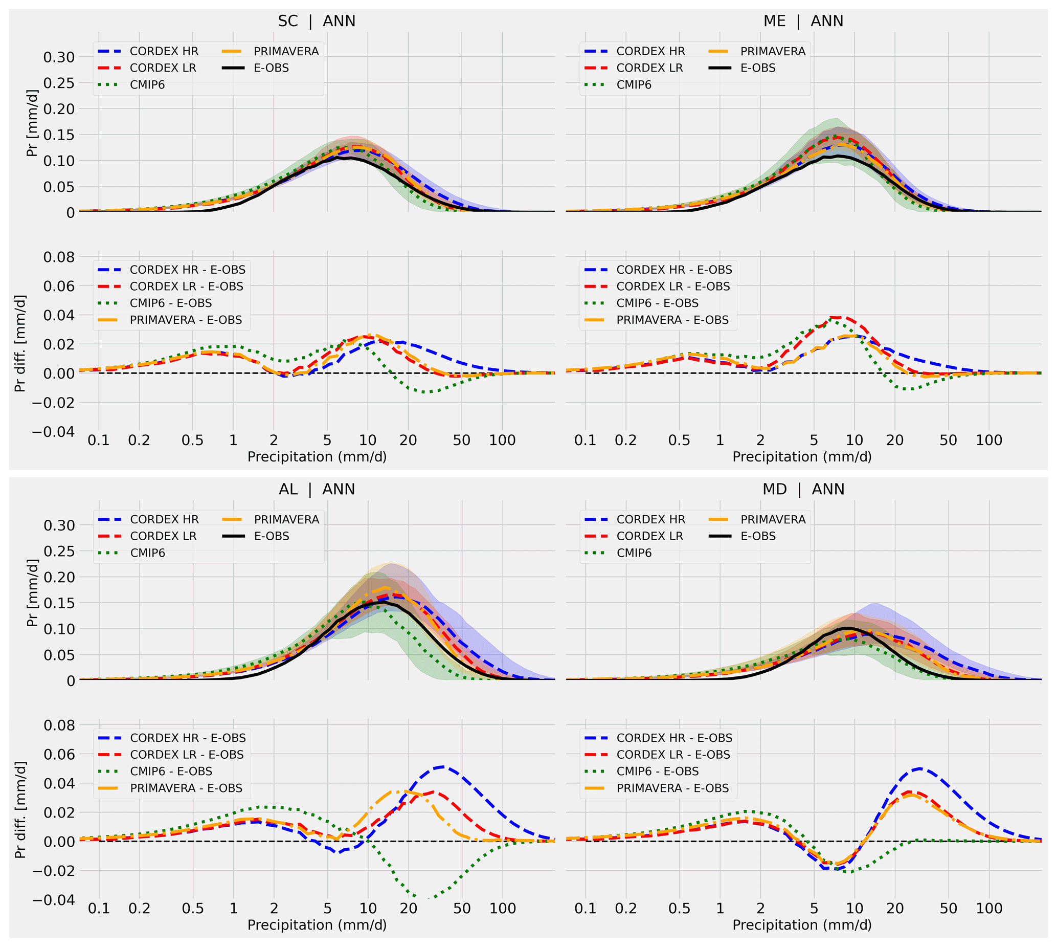
Figure 2 The panels show the actual contribution (to the total median precipitation, y axis) per precipitation intensity bin (x axis), based on annual (ANN) daily precipitation values in the CMIP6 (green dotted lines and shading), PRIMAVERA (orange dashed–dotted lines and shading), CORDEX low-resolution (red dashed lines and shading), and CORDEX high-resolution (blue dashed lines and shading) ensembles. The displayed regions are Scandinavia (SC, top left), mid-Europe (ME, top right), the Alps (AL, bottom left), and the Mediterranean (MD, bottom right). Coloured shadings represent the 5–95th percentile range in respective ensemble. Black solid lines are E-OBS (0.1^∘ resolution) observations.

3.1.2 Seasonal precipitation

Further insight can be gained by investigating seasonal differences (Fig. 3). In winter (DJF) the model ensemble means generally overestimate total mean precipitation compared to E-OBS (i.e. total areas under the curves showing differences are positive). The bulk of the distributions are slightly shifted to higher precipitation rates and also to higher contributions (except for the Mediterranean region). The largest inter-ensemble differences are seen for the Mediterranean where CORDEX HR shows the largest shift from E-OBS towards contributions from higher precipitation rates, and PRIMAVERA is similar to CORDEX LR. In summer (JJA), the ensemble means show larger contributions from intensities above 10–15 mm d⁻¹ than E-OBS, especially in CORDEX HR. However, as this is in many cases compensated for by lower contributions from rates between 2–10, the total mean precipitation biases are smaller than in winter. While the CORDEX ensemble means indicate larger total mean precipitation in France and the Mediterranean, CMIP6 produces higher contributions from low to moderate ($<\sim \mathrm{5}$ mm d⁻¹) in all regions compared to E-OBS and lower contributions from higher intensities. Furthermore, there is a tendency in all regions of a larger spread within each model ensemble in JJA than in DJF (see coloured shadings in Fig. 3). Even though it is a very crude estimate of the spreads (the 5–95th percentile range in the respective model ensemble), it can be argued that the differences in part are related to the seasonally prevailing weather conditions. In winter the North Atlantic storm track is in its active phase, with frequent passings of synoptic weather systems over Europe. These features are generally well represented in climate models – hence larger consistency with associated precipitation across models. In summer, on the other hand, synoptic activity is reduced and convective processes (either as isolated or organised systems or embedded in larger-scale features like fronts) become more prominent in precipitation events. Sensitivity to model grid resolution and physics parameterisations (e.g. convection parameterisation) is larger during this season. The larger summertime spread in ensembles seen in Fig. 3 might then reflect larger uncertainties associated with model resolution and formulation. It is further noted that the ensemble spread is not increased as much (from winter to summer) over northern and north-western Europe, which is relatively more affected by synoptic-scale events during summer compared to southern parts of Europe (not shown).

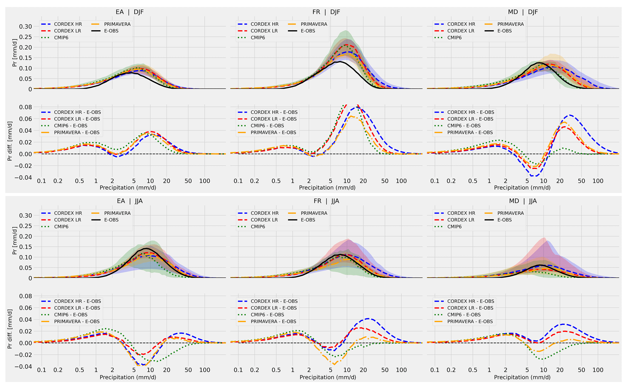
Figure 3 Same as in Fig. 2 but for DJF (top row) and JJA (bottom row) daily precipitation values and for the eastern Europe (EA, left), France (FR, middle), and Mediterranean (MD, right) regions. Coloured shadings represent the 5–95th percentile range in respective ensemble. Black solid lines are E-OBS (0.1^∘ resolution) observations.

Model ensemble differences for all regions and seasons are summarised in Fig. 4, with E-OBS as reference. In spring (MAM) and winter (DJF) all ensembles have higher total mean precipitation in all regions. In summer (JJA) and autumn (SON) biases are also mostly on the positive side but smaller (primarily for GCM ensembles) and in some regions close to zero or slightly negative (e.g. the Alps, eastern Europe, Iberian Peninsula). Often there is an indication of a positive correlation between differences in mean (x axis in Fig. 4) and differences in fractional contributions (y axis, which indicates overall differences in the shape of the distributions), as seen for example in France or mid-European regions. However, there are also cases with large differences in the shape but small total mean precipitation biases, for example the CMIP ensembles in JJA and SON over the Alps, suggesting compensating effects from different parts of the precipitation distribution. The overall spread is also highly variable between the regions; Scandinavia, mid-Europe, and eastern Europe and the British Isles are characterised by relatively smaller inter-ensemble differences, while in the Alps and Mediterranean the spread is large. The spread is in some regions dominated by inter-seasonal differences, e.g. in Mid-Europe and France, where typically the largest differences (in terms of both total means and distribution shapes) occur in DJF and MAM and smaller spreads in JJA and SON. In the Alps, Iberian Peninsula, and the Mediterranean regions, however, the relatively larger inter-ensemble differences lead to an increased overall spread. Here, CORDEX HR further exhibits the largest differences to the GCM ensembles and also often larger deviations from E-OBS. These latter regions are either characterised by complex and steep topography (e.g. the Alps and the Pyrenees), a large fraction of coastal areas, and/or by relatively dry environments dominated by precipitation of convective nature (particularly for the warmer months). These factors most likely play important roles for the larger differences seen between the low-resolution CMIP GCMs and the higher-resolution PRIMAVERA GCMs and CORDEX RCMs, as well as contributing to larger uncertainties in, and lower quality and representativeness of, observational data. In contrast, in almost all seasons over the British Isles, the CORDEX HR biases in total precipitation compared to E-OBS are among the smallest with respect to the other ensembles (the difference in the shape is similar). Finally, it is noted that for all regions PRIMAVERA HR and CORDEX LR give comparable distributions as they are of similar resolution.

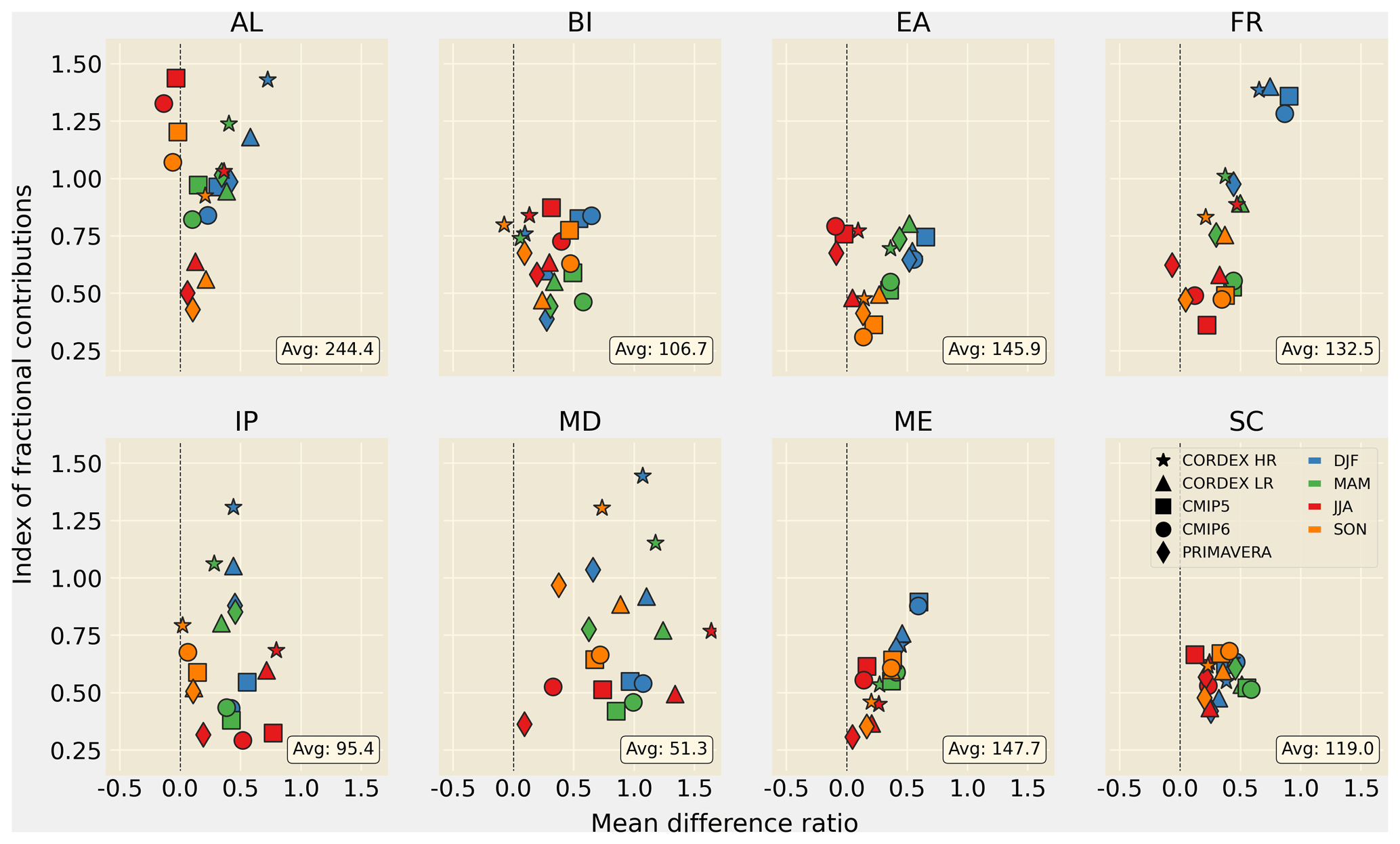
Figure 4 The index of fractional contributions (y axis) plotted as a function of the fractional difference in seasonal total precipitation (x axis). E-OBS (0.1^∘ resolution) is the reference data set, and E-OBS average annual total precipitation (mm yr⁻¹) is shown in lower right in each panel.

To summarise, we can conclude that, in comparison to E-OBS, most model ensembles exhibit larger contributions for most precipitation intensities, but most consistent for low (< ca. 3 mm d⁻¹) and moderate to high (> ca. 10 mm d⁻¹) intensities. The larger contributions occur predominantly in DJF while in summer there are often lower contributions than in E-OBS for moderate intensities (leading to smaller biases in total means). In general, the CORDEX ensembles, and most often also PRIMAVERA, show a shift towards larger contributions from higher intensities compared to CMIP ensembles, especially in areas with complex orography as in the Alps. The higher model grid resolution does not always lead to improvements, i.e. closer agreements to E-OBS. However, it is worth re-emphasising that the quality of E-OBS observations can be significantly lower in certain regions (e.g. mountainous areas or areas with low density of precipitation gauges) and seasons (especially in wintertime when the fraction of snowfall is largest, which is more sensitive to wind-induced undercatch) (Prein and Gobiet, 2017; Herrera et al., 2019), thus complicating the assessment of model behaviour in comparison to observations. To further highlight this issue, we have included an ASoP analysis for the Scandinavia region (Fig. S3) including a regional high-quality high-resolution gridded observational data set: NGCD (Lussana et al., 2018). In both DJF and JJA, the model ensembles still overestimate contributions from the bulk of the intensity distribution; however, NGCD has higher contributions from low intensities compared to E-OBS, reducing the model ensemble bias. More interestingly, NGCD shifts towards larger contributions for high intensities, >10 mm d⁻¹, in effect lending more credibility to the CORDEX HR ensemble and less to the others.

Figure 5 The panels show the actual contribution (to the total mean precipitation, y axis) per precipitation intensity bin (x axis), based on DJF (top row) and JJA (bottom row) daily mean precipitation values in CORDEX and PRIMAVERA models for the Scandinavian (SC), British Isles (BI), Alps (AL), and Iberian Peninsula (IP) regions. Thin lines in the upper part of each panel represent each individual model while the thick lines represent the ensemble means. In the lower part of each panel each line represents differences between respective high- and low-resolution model pairs.

3.1.3 Effect of grid resolutions – a one-to-one comparison

For multi-model ensembles, the sensitivity to model grid resolutions can generally only be assessed qualitatively since other aspects, such as differences in model formulation, also contribute to differences in model performance. In other words, it cannot be definitely stated to what extent differences in performance comes from higher resolution or from other differences in the model code. For the PRIMAVERA models, however, it is possible to directly compare low- and high-resolution model versions. In CORDEX ensembles this is also possible to some extent for a few models where low- and high-resolution versions of RCMs have been forced by the same parent GCMs. This is the case for nine RCM-GCM combinations (six different RCMs driven by four different GCMs). Note that, in contrast to PRIMAVERA, CORDEX LR–HR “pairs” may not use the same version of the common model, which could also influence the results in addition to change in grid resolution. Further, the magnitude of the grid resolution change (the δ value) is the same for CORDEX models (δ=4), while for PRIMAVERA models it varies between approximately 2 and 5. Figure 5 shows the one-to-one comparison for DJF and JJA for selected regions. For CORDEX models the high-resolution model versions generally generate, in both seasons, larger contributions from precipitation intensities above ca. 10 mm d⁻¹. This is sometimes accompanied by lower contributions from lower rates as seen for example in Scandinavia and the Alps in DJF. Similar results are seen for PRIMAVERA, although not as consistently; e.g. over the British Isles and the Alps in JJA about half the models show increased contributions in the HR models over the bulk part, with the other half showing instead lower contributions (although for higher rates most HR models show larger contributions). In fact, for many regions there is a larger spread in JJA within each model ensemble and also between the individual LR versus HR responses compared to DJF. It could be argued that this effect is related to precipitation events being of a more convective nature in summer and thus having a larger sensitivity to model grid resolution as well as model physics. In winter, CORDEX RCMs are to a larger extent being influenced by the forcing GCMs and therefore, as there are only four different GCMs used in the nine RCM–GCM combinations shown here, tend to exhibit more similar responses in this season.

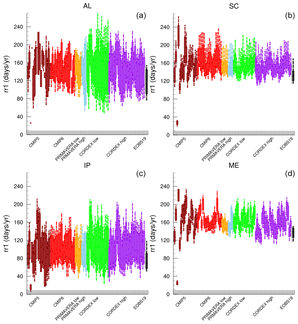
Figure 6 Number of precipitation days (RR1, d yr⁻¹) in the Alps (AL, a), Scandinavia (SC, b), the Iberian Peninsula (IP, c), and mid-Europe (ME, d) for individual models in the CMIP5 (brown), CMIP6 (red), PRIMAVERA LR (orange), PRIMAVERA HR (light blue), CORDEX LR (green), and CORDEX HR (purple) ensembles as well as E-OBS at 28 km (grey) and 11 km (black). Boxes mark the 25th and 75th percentiles, with the median inside; whiskers go from the 10th to the 90th percentile.

3.2 Selected precipitation-based indices

3.2.1 Model ensemble comparison

Figure 6 shows the number of precipitation days (RR1, Table 3) as simulated by all models for each PRUDENCE region. The number of precipitation days does not differ much between the model ensembles. There are clear differences between individual models, but it is difficult to establish any significant differences between the model ensembles. This is the case both for regions with a higher occurrence of precipitation days (e.g. SC) and regions with fewer precipitation days (e.g. IP). All models show about the same number of precipitation events over the whole year, which may suggest that the large-scale weather patterns are not influenced that much by higher resolution; also, when looking at individual seasons the differences between ensembles are small (Fig. S4). Note, however, that the large-scale circulation in the RCMs to a large extent is governed by the driving GCMs which have typical resolutions of around 200 km. Interpolating the data to a common grid prior to analysis does not have a large impact on RR1 (Fig. S5). Most models overestimate the number of precipitation days compared to observations. It is a well-known feature of climate models, particularly those with parameterised convection, that they tend to have too many wet days (e.g. Dai, 2006; Stephens et al., 2010).

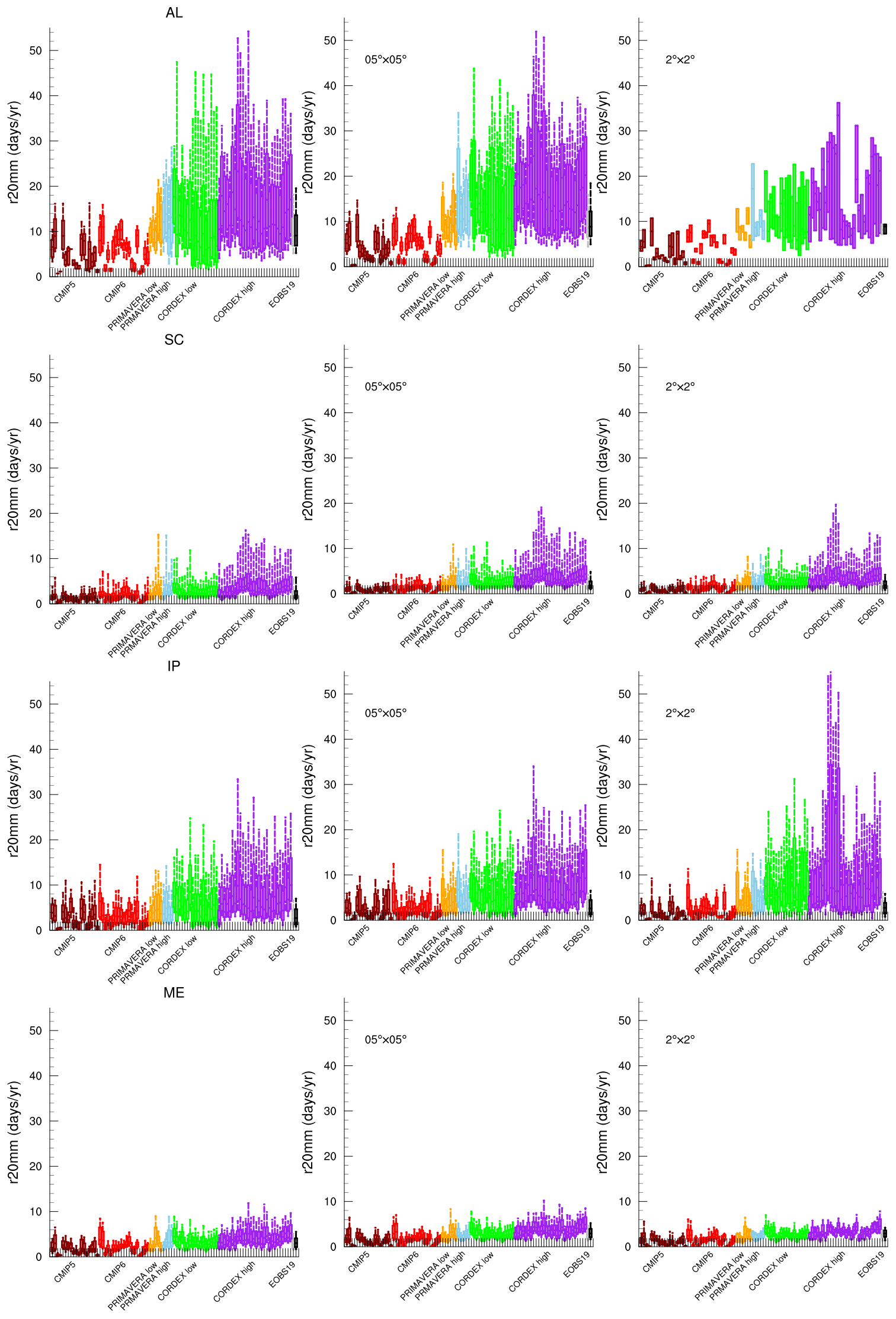
Figure 7 Same as Fig. 6 but for the number of days with precipitation amount over 20 mm (R20mm, d yr⁻¹). Left column: model data on their original grids; centre column: all data regridded to $\mathrm{0.5}{}^{\circ }\times \mathrm{0.5}{}^{\circ }$ grid; right column: all data regridded to $\mathrm{2}{}^{\circ }\times \mathrm{2}{}^{\circ }$ grid.

The number of days with large precipitation amounts, above 10 and 20 mm d⁻¹, become more frequent with higher model resolution. For example, the number of days with precipitation over 20 mm (R20mm, Table 3) increases from just a few in CMIP5 to 5–10, or even more, in CORDEX HR (Fig. 7). The 10th to 90th inter-percentile range increases, due to a larger increase in the 90th percentile. Generally, the spread is larger for models with high resolution. This could partly be explained by the higher number of data points in the high-resolution models (i.e. larger number of grid points); a high-resolution model is more likely to better represent the spatial variations in precipitation within a region while in coarser-scale models precipitation fields are smoother due to fewer grid points. The differences between resolutions remain, however, also when all data are interpolated to two common grids of $\mathrm{0.5}{}^{\circ }\times \mathrm{0.5}{}^{\circ }$ and $\mathrm{2}{}^{\circ }\times \mathrm{2}{}^{\circ }$ resolutions; the median and spread also remain similar in all ensembles. In small regions such as the Alps the coarsest grid gives too few points, which means that it is difficult to calculate the 10th and 90th percentiles. The spread in CORDEX HR increases when interpolated to $\mathrm{2}{}^{\circ }\times \mathrm{2}{}^{\circ }$ because the points with high values are not balanced by as many points close to the median (a $\mathrm{0.5}{}^{\circ }\times \mathrm{0.5}{}^{\circ }$ grid contains 16 times more points than a $\mathrm{2}{}^{\circ }\times \mathrm{2}{}^{\circ }$ grid). Compared to E-OBS the average number of days with more than 20 mm d⁻¹ is more accurately simulated in the high-resolution ensembles, but the spread is highly exaggerated. The PRIMAVERA models have median values similar to E-OBS and also a more similar spread. The signal is the same for the individual seasons but less pronounced since the potential number of days is smaller when divided over four seasons instead of counted over the whole year (Fig. S6). The effect of resolution is therefore clearest in the season when most days occur, which means winter in western Europe and summer in central Europe.

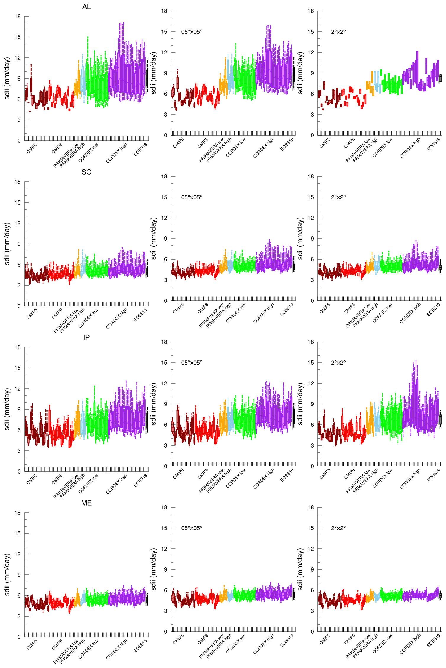
The fact that the number of wet days is similar between LR and HR models (Fig. 6) but with increased frequency of (heavy) precipitation in HR models (Fig. 7) suggests that, for the latter, the precipitation intensity on the wet days is higher. This is shown in the simple precipitation intensity index (SDII, Table 3, Fig. 8). SDII is indeed affected by resolution, at least between CMIP5–CMIP6 and CORDEX; the wet day average precipitation is larger in the HR simulations compared to LR models, and also the intra-model spread (spread between models within the ensemble) is larger. For all regions, SDII is higher in the HR models. Perhaps the relative increase in SDII is higher in regions with large spatial variations (for example because of complex orography or coastlines) such as the Iberian Peninsula and the Alps. The median SDII values in high-resolution models are closer to E-OBS than the low-resolution models in all regions, even though the model spread is generally larger in the climate models than in E-OBS. The differences between ensembles remain for both the median and the spread when the data are regridded to common grids. Also, for individual seasons it is clear that SDII increases with higher resolution, but the SDII values do not vary much with season (Fig. S7).

Figure 8 Same as Fig. 7 but for the simple precipitation intensity index (SDII, mm d⁻¹).

The higher intensities for extreme precipitation in high-resolution models compared to low-resolution models are also seen in the maximum 1 d (Rx1day, Table 3, Fig. 9) and maximum 5 d precipitation (not shown). There is a clear increase in both intensities and intra-model spread in the high-resolution models. It can be discussed whether this increase is an improvement since the CORDEX HR models give a maximum 1 d precipitation that is significantly larger than E-OBS. On the other hand, it can be discussed whether E-OBS is able to reliably represent these extremes (Hofstra et al., 2009; Prein and Gobiet, 2017). The medians and the spreads remain more or less the same when also regridded to common grids. In small regions such as the Alps the spread is reduced because the number of data points is small when regridded to a coarse grid. In regions with large spatial variations (e.g. between coast and mountain) such as Iberian Peninsula the spread increases because high values are not balanced by as many points with values close to the median. In winter the effect of higher resolution is mainly seen in regions with complex topography, while in summer there is a clear signal in all regions (Fig. 10). This reflects that higher resolution makes the largest difference in complex topography and for convective precipitation events.

Figure 9 Same as Fig. 7 but for the maximum 1 d precipitation (Rx1day, mm d⁻¹).

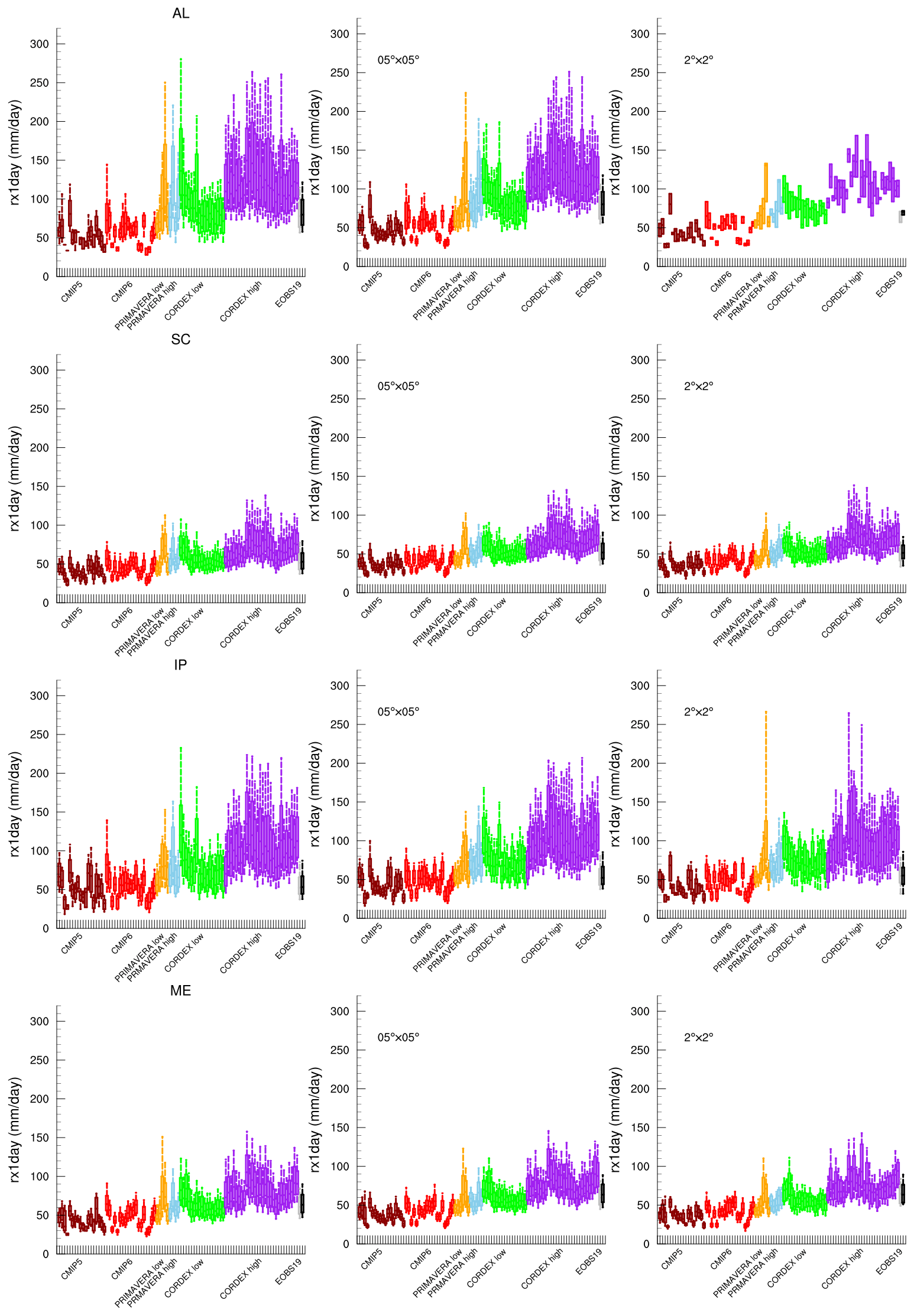
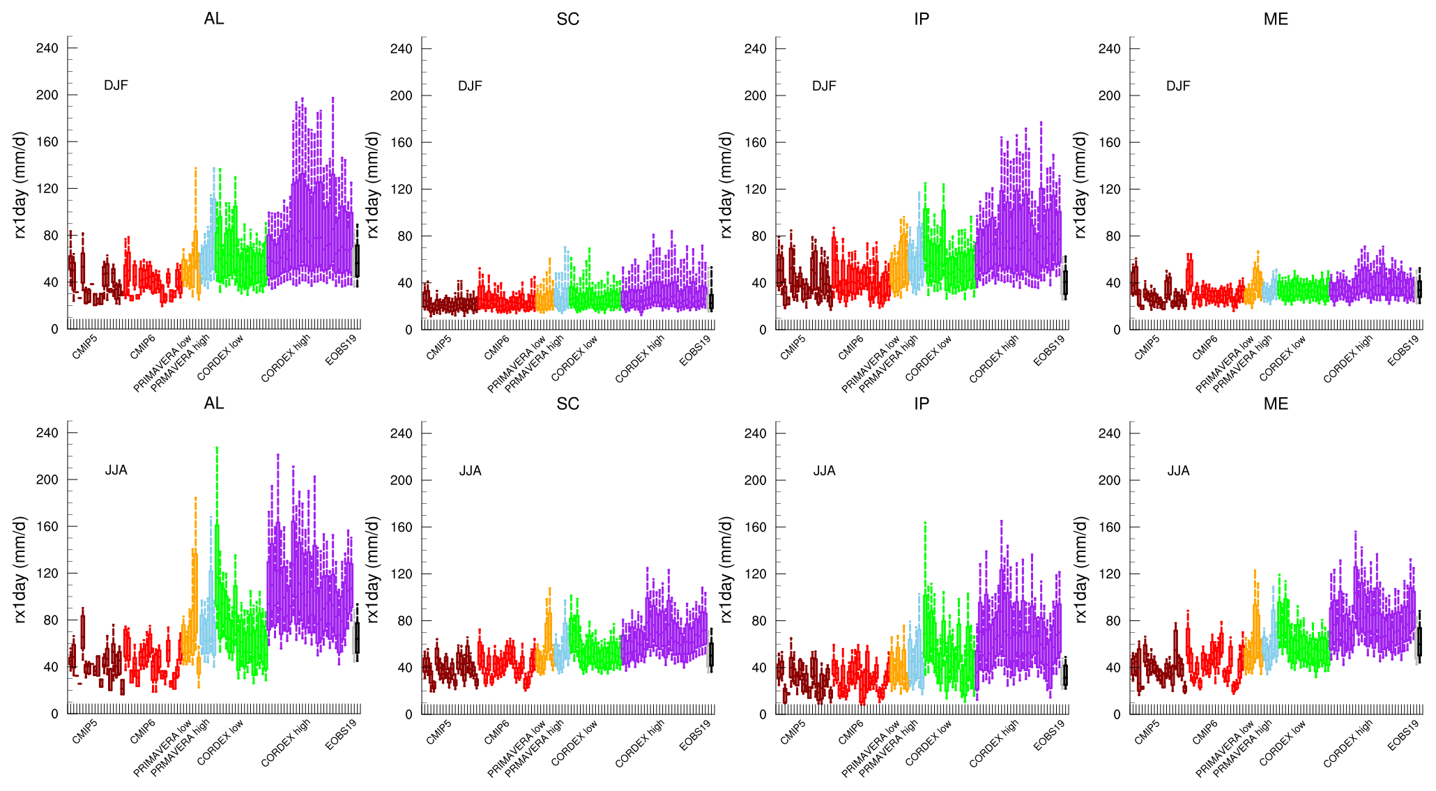
Figure 10 Same as Fig. 6 but for the maximum 1 d precipitation (Rx1day, mm d⁻¹): top row: winter (DJF); bottom row: summer (JJA).

3.2.2 One-to-one comparison

We let the mid-European region (ME) represent the whole domain, as the same conclusions can be made for all regions, only with small differences in the number of models that give significant differences. A one-to-one comparison is made of the selected indices for the models where there is both a low- and a high-grid-resolution version (Fig. 11). The LR and HR versions are compared with a Welch t test (Welch, 1947) at the 0.05 significance level to see whether the simulated indices are significantly different. This corroborates the analysis above and adds further detail by quantifying the differences.

Figure 11 Number of precipitation days (RR1, d yr⁻¹, first row), number of days with precipitation amount over 20 mm (R20mm, d yr⁻¹, second row), simple precipitation intensity index (SDII, mm yr⁻¹, third row), maximum 1 d precipitation (Rx1day, mm d⁻¹, fourth row) in the mid-European region (ME) in the PRIMAVERA LR (pink) and HR (red) models, CORDEX LR (light blue) and HR (purple) models, and E-OBS LR (grey) and HR (black). Left column: model data on their original grids; centre column: all data regridded to $\mathrm{0.5}{}^{\circ }\times \mathrm{0.5}{}^{\circ }$ grid; right column: all data regridded to $\mathrm{2}{}^{\circ }\times \mathrm{2}{}^{\circ }$ grid. Boxes mark the 25th and 75th percentiles, with the median inside; whiskers go from the 10th to the 90th percentile. If the high-resolution version of a model is significantly different from the low-resolution version, this is marked with a vertical line in the high-resolution boxes.

Although the difference in the number of precipitation days (RR1, Fig. 11, top row) is significant for most models, it is not clear how it is affected by resolution. The differences are small, mainly within ±10 d yr⁻¹, in some cases negative and in some positive. The differences between models are larger than the differences between resolutions. It is clear, however, that all models overestimate the number of precipitation days compared to E-OBS. This is true also when the data are regridded to common grids, but three models and E-OBS get insignificant differences when regridded to $\mathrm{2}{}^{\circ }\times \mathrm{2}{}^{\circ }$ instead of only one model at the native grids.

The number of days with precipitation more than 20 mm (R20mm, Fig. 11, second row) is significantly different between HR and LR for all models and E-OBS. For the CORDEX models R20mm is higher in most HR versions, while the difference is less clear in the PRIMAVERA models. All simulations with the RCA4 RCM, regardless of the driving GCM, clearly show higher R20mm in the HR version compared to the LR versions, which indicates that the difference in the index is mainly a result of the changed grid resolution in the RCM. The differences between LR and HR also remain when regridded to common grids, which means that this is an effect of differences in model physics. CORDEX LR is close to E-OBS, while CORDEX HR generally overestimates R20mm.

The simple precipitation intensity index (SDII, Fig. 11, third row) is significantly different in one out of four PRIMAVERA models and four out of nine CORDEX models. Differences are small, tenths of mm d⁻¹, for most models. Most significant differences disappear when regridded to $\mathrm{0.5}{}^{\circ }\times \mathrm{0.5}{}^{\circ }$ and all disappear when regridded to $\mathrm{2}{}^{\circ }\times \mathrm{2}{}^{\circ }$, suggesting that the resolution does not affect SDII much in these model pairs. We still see a difference between CMIP GCMs and CORDEX RCMs (see Fig. 8).

The maximum 1 d precipitation (Rx1day, Fig. 11, bottom row) is significantly different in the HR version in all but one model (a PRIMAVERA model). The HR versions have higher precipitation values and larger spread in all but two PRIMAVERA models and one CORDEX model. In particular the CORDEX HR models have a higher maximum 1 d precipitation. This seems to be driven by the RCM rather than the driving GCM. As an example, three RCMs are forced with the MPI-ESM-LR GCM. When forced by this GCM the Rx1day in the CCLM4-8-17 RCM is lower in the HR version, while in REMO2009 and RCA4 HR RCMs Rx1day is higher. In RCA4 the difference is particularly large, regardless of the driving GCM. That the differences result from differences in model physics is supported by the fact that the differences also remain when the data are regridded to common grids.

The one-to-one comparison of selected indices shows that there are significant differences between the LR and HR models and that these are results of differences in model performance and not only the number of data points. It also shows that for some indices the largest difference occurs between CMIP5–CMIP6 and PRIMAVERA HR, rather than between PRIMAVERA and CORDEX. This means that some of the differences seen in Figs. 6–10 are not as clear in Fig. 11. The comparison also shows that even though there are significant differences between LR and HR, for some cases it is difficult to establish significant differences between two ensembles since the difference between two models is often larger than between the LR and HR versions of the same model.

It should be noted that the CORDEX RCMs are not always run with the same model version in the LR and HR simulations. Model differences could thus explain some of the differences between LR and HR. Since we do not have LR and HR simulations with all model versions, we cannot quantify this effect, only acknowledge it. It should also be noted that the difference in horizontal grid spacing varies between models. For CORDEX RCMs the resolution δ (LR divided by HR) is always 4 (50 km divided by 12.5 km), but for PRIMAVERA it varies between 2 and 5. The δ value is larger in CORDEX than in most PRIMAVERA models, which could potentially mean that the effect of resolution is overestimated for the CORDEX RCMs. Figure 12 shows how the absolute differences in RR1, R20mm, SDII, and Rx1day between the LR and HR versions of the PRIMAVERA and CORDEX models described above correlate to the δ value in the ME region. There is no clear relation between the δ value and the size of the difference. CORDEX models that all have the same δ value span from small to large differences. The spread between PRIMAVERA models is also quite large. This again suggests that the response of a model to increased resolution depends on the model itself and not only on the magnitude of the resolution change.

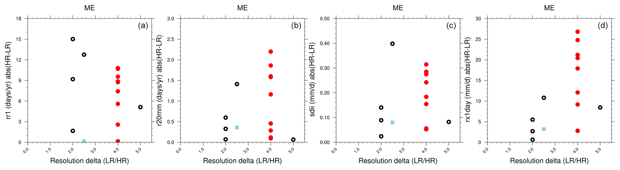
Figure 12 Absolute difference between HR and LR version of PRIMAVERA (black rings), CORDEX (red circles), and E-OBS (blue squares) in precipitation days (RR1, d yr⁻¹, a), number of days with precipitation amount over 20 mm (R20mm, d yr⁻¹, b), simple precipitation intensity index (SDII, mm d⁻¹, c), and maximum 1 d precipitation (Rx1day, mm d⁻¹, d) in the mid-European region (ME). The x axes show the resolution delta (LR divided by HR) for each model (example: 50 km grid spacing divided by 12.5 km equals 4).

4 Discussion and conclusions

This study investigates the importance of model resolution on the simulated precipitation in Europe. The aim is to investigate the differences between models and model ensembles but also to evaluate their performance compared to gridded observations. In a similar study Demory et al. (2020) compare PRIMAVERA models with CORDEX LR and CORDEX HR. They conclude that CORDEX indisputably improves the data from the driving CMIP5 models but that the differences between CORDEX LR and PRIMAVERA are generally small. Both ensembles perform well but tend to overestimate precipitation in winter and spring. The largest differences between the ensembles are for high precipitation intensities, especially in summer, where PRIMAVERA gives less heavy precipitation, which makes it agree more with observations than CORDEX. Iles et al. (2020) compare the effect of resolution on extreme precipitation in Europe in CMIP5 GCMs and CORDEX RCMs. They conclude that high-resolution models systematically produce higher frequencies of high-intensity precipitation events. Our interpretation of this, given the results in our study, is that in some cases the overestimation of precipitation compared to E-OBS also increases with higher resolution. The findings in this study support the conclusions from the above-mentioned studies and add details based on a wider range of model ensembles and precipitation metrics. The fact that we come to the same conclusions as Iles et al. (2020) and Demory et al. (2020) with slightly different methods gives strength to these conclusions.

The ASoP analysis in this study shows that all model ensembles have larger contributions from heavy precipitation in winter compared to E-OBS and that the higher values become most prominent for the ensemble with the highest grid resolution, CORDEX HR. The biases compared to E-OBS are generally smaller in summer. The PRIMAVERA ensemble is in good agreement with observations and has smaller bias than CORDEX for many regions. CMIP5 and CMIP6 mostly underestimate contributions from moderate to high precipitation intensities in summer while overestimating low-intensity events. Overall, in the summer season, the spread is large between ensembles and between models within the ensembles. This is indicative of large uncertainties which are most likely related to uncertainties in how models are able to treat smaller-scale precipitation events involving convection. With respect to E-OBS, the ASoP results partly show that higher horizontal grid resolution does not necessarily mean better. However, in coastal regions and regions with steep or complex topography, there are uncertainties in both models and observations. Particularly in winter, observations suffer from undercatch when precipitation falls as snow during windy conditions, and in summer, smaller-scale convective precipitation may be smoothed considerably or missed completely by ground rain gauges (which E-OBS is based on). E-OBS is not based on the full network of rain gauges in all countries, which could also lead to undercatch. Therefore, it is not always obvious which model or ensemble of models is closest to reality. When compared to NGCD, a regional data set of high quality, the difference between CORDEX HR and observations is reduced, which gives more confidence to the high-resolution model results.

It is clear that the horizontal resolution of a model has a large effect on precipitation, mostly on the heavier precipitation and in areas with complex and steep orography. The number of precipitation days does not depend much on resolution as this mostly depends on large-scale weather patterns and not so much on local topography and convection. For heavy-precipitation events, which often are more local and short-lived in character, model resolution is more important. The high-resolution models better resolve such events and distinguish better between different parts of a region. Thus, extreme precipitation is more intense and more frequent in the HR models compared to the LR models in this study. With the same amount of wet days this means that precipitation intensifies so that the wet days get wetter. The largest impact of increased model-scale resolution on precipitation is most evident for the coarser-scale models; increasing the resolution from CMIP5–CMIP6 to PRIMAVERA HR has a greater effect than increasing from CORDEX LR or PRIMAVERA HR to CORDEX HR. This does not, however, mean that increased resolution gets less and less worthwhile; further refining the grid until convection-permitting resolutions are reached (less than ∼5 km grid spacing), in which case convection parameterisations may be turned off, has a large positive effect (e.g. Prein et al. 2015). This is not shown here as the smallest grid spacing in models in this study is 12.5 km. The effect of higher resolution is seen in regions with small amounts of precipitation as well as regions with high amounts of precipitation, and in regions with small and large geographical differences. The higher percentiles change more than the low percentiles for all studied indices. Increasing resolution has about the same effect on both GCMs and RCMs; furthermore GCMs and RCMs of comparable resolution simulate comparable precipitation climates, even though PRIMAVERA is often drier than CORDEX.

It is worth noting that the differences between RCM simulations, and how they respond to differences in resolution, may very well be explained by the driving GCM and the state of the atmospheric general circulation in them (Kjellström et al., 2018; Sørland et al., 2018; Vautard et al., 2020). Higher resolution is expected to give a better described and more detailed climate, with for example deeper cyclones and more intense local showers, in a sense with more pronounced weather events. If two models are in different states, for example when it comes to where storm tracks cross Europe, and if these states are pronounced, that may lead to even larger model differences. Instead of a weak storm track in the south and a weak storm track in the north in the low-resolution model, we may now instead have strong storm tracks, which mean that the difference between the models increases. Still, the largest differences are seen in the CORDEX ensemble where the LR and HR models are run with the same coarse-resolution GCM. This suggests that (regional) model resolution and performance is what determines high precipitation rates, rather than the driving GCM. To fully answer that would require an analysis of the circulation patterns in the different models. This is not done here but should be a topic for further studies.

The differences between LR and HR largely also remain when the results are regridded to common grids of $\mathrm{0.5}{}^{\circ }\times \mathrm{0.5}{}^{\circ }$ and $\mathrm{2}{}^{\circ }\times \mathrm{2}{}^{\circ }$, which means that the HR version performs differently than the LR version of the same model, mainly because of better representations of topography and convection. The largest seasonal differences are seen for heavy precipitation (R20mm, Rx1day). Heavy-precipitation events usually occur locally in summer, which makes it more sensitive to model resolution. Difference in resolution has a larger impact on heavy precipitation in summer than in winter.

Higher resolution does not necessarily mean better results. If a model is already too wet, the increase in heavy precipitation that is induced by the higher resolution means that the HR version agrees less with observations than the LR version. For the individual model it is possible to quantify the difference and improvement between LR and HR. On the ensemble level this is more difficult. The difference between different models is often larger than between LR and HR versions of the same model. In this sense the quality of an ensemble depends more on the models it consists of rather than the average resolution of the ensemble. Furthermore, when downscaling with an RCM, the simulated extreme precipitation, and the differences between GCM and RCM, depends more on the used RCM and less on the down-scaling itself, especially for heavy precipitation and particularly in summer.