Origins of multi-decadal variability in sudden stratospheric warmings

Sudden stratospheric warmings (SSWs) are major disruptions of the Northern Hemisphere (NH) stratospheric polar vortex and occur on average approximately six times per decade in observation-based records. However, within these records, intervals of significantly higher and lower SSW rates are observed, suggesting the possibility of low-frequency variations in event occurrence. A better understanding of factors that influence this decadal variability may help to improve predictability of NH midlatitude surface climate, through stratosphere–troposphere coupling. In this work, multi-decadal variability of SSW events is examined in a 1000-year pre-industrial simulation of a coupled global climate model. Using a wavelet spectral decomposition method, we show that hiatus events (intervals of a decade or more with no SSWs) and consecutive SSW events (extended intervals with at least one SSW in each year) vary on multi-decadal timescales of periods between 60 and 90 years. Signals on these timescales are present for approximately 450 years of the simulation. We investigate the possible source of these long-term signals and find that the direct impact of variability in tropical sea surface temperatures, as well as the associated Aleutian Low, can account for only a small portion of the SSW variability. Instead, the major influence on long-term SSW variability is associated with long-term variability in amplitude of the stratospheric quasi-biennial oscillation (QBO). The QBO influence is consistent with the well-known Holton–Tan relationship, with SSW hiatus intervals associated with extended periods of particularly strong, deep QBO westerly phases. The results support recent studies that have highlighted the role of vertical coherence in the QBO when considering coupling between the QBO, the polar vortex and tropospheric circulation.

1 Introduction

Major sudden stratospheric sudden warming (SSW) events involve significant disruption of the Northern Hemisphere (NH) stratospheric polar vortex and represent the largest mode of interannual variability in the boreal winter stratosphere (Butler et al., 2017; Baldwin et al., 2021). They are associated with an equatorward shift and deceleration of the North Atlantic jet stream (Kidston et al., 2015), negative phases of the North Atlantic Oscillation (NAO) (Baldwin and Dunkerton, 2001) as well as cold snaps over Eurasia and North America (Thompson, 2003; Lehtonen and Karpechko, 2016; Tomassini et al., 2012; Kretschmer et al., 2018). SSWs also play a key role in seasonal to subseasonal forecasts (Domeisen et al., 2020a, b). In reanalysis datasets, SSWs occur at an average rate of 0.6 events per winter but this varies markedly over the record (Butler et al., 2015), suggesting the possibility of variability on much longer timescales. For example, observational studies have noted a hiatus in the 1990s when very few major SSW events occurred (Butler et al., 2015; Pawson and Naujokat, 1999; Shindell et al., 1999). This is estimated to be the longest such interval since 1850 (Domeisen, 2019). In contrast, the early 21st century displayed a remarkable number of consecutive winters containing SSW events (Manney et al., 2005).

Despite a significant body of work aimed at understanding the nature of SSWs and their impacts on midlatitude surface climate, variability of their occurrence on decadal to multi-decadal timescales is not well understood. Multi-decadal stratospheric variability has been considered in the context of forced anthropogenic warming signals in global climate models (GCMs). For example, Garfinkel et al. (2017) analysed decadal-scale variations in polar vortex strength in a set of historical simulations and proposed that an observed hiatus in Eurasian surface warming was most likely due to variability in midwinter vortex strength. Similarly, Cohen et al. (2009) found decadal-scale variations in planetary wave forcing of the vortex in a suite of Coupled Model Intercomparison Project phase 3 (CMIP3) models as well as National Centers for Environmental Prediction – National Center for Atmospheric Research (NCEP–NCAR) reanalysis. They suggest these fluctuations lead to a modulation of the global warming signal in late boreal winter surface temperatures. Whether the vortex variability was forced by greenhouse gas concentrations or arose through internal variability in these studies was not fully established, but Garfinkel et al. (2015) used a subset of the simulations analysed in Garfinkel et al. (2017) and linked a decadal trend (1980–2009) in late winter vortex strength to sea surface temperature (SST) variability. On the other hand, Seviour (2017) analysed observed variations between 1980 and 2016 and concluded that the vortex variability was primarily internally generated. Schimanke et al. (2011) noted multi-decadal-scale variations in SSW occurrence with periods of approximately 52 years in a multi-century GCM integration and demonstrated coherent variability in other parts of the climate system, including vertically propagating planetary wave activity, Eurasian snow cover and Atlantic SSTs. However, despite providing some indications of externally driven variability, results from this study are not conclusive, since the GCM used (EGMAM: ECHO-G with Middle Atmosphere Model) exhibits significant bias in mean SSW rate compared to reanalyses (two events per decade). This means that their findings may not be fully representative of the observed stratosphere, and the authors note that further simulations are required to understand this variability. Manzini et al. (2012) explored causes of 20-year period variability in a simulation with prescribed pre-industrial SSTs. They propose that, given the boundary conditions in the simulations are fixed, such variability must be internally generated. Butchart et al. (2000) suggest that decadal variability in vortex strength as well as SSW frequency may originate from feedbacks caused by the non-linear nature of boreal winter stratospheric dynamics. Both works show that these internally induced signals significantly influence midlatitude surface variability, forcing similar period signals in the NAO and North Atlantic SSTs.

A region often considered in studies of vortex strength variability is the equatorial stratosphere. The primary mechanism for coupling between these regions is between the quasi-biennial oscillation (QBO) and the vortex. An association between the phase of the QBO and the strength of the polar vortex was first proposed by Holton and Tan (1980) and Holton and Tan (1982), who found that the polar vortex exhibited a strengthening when the QBO near the 50 hPa level was in its westerly phase (QBO-W) compared to its easterly phase (QBO-E). This link, usually referred to as the Holton–Tan (HT) effect, has been reported in subsequent studies with more comprehensive observations as well as in modelling studies using GCMs including the Met Office Hadley Centre Model version 2 (HadGEM2) (Watson and Gray, 2014) and other Met Office models (Garfinkel et al., 2018) based on predecessors of the model considered in this study. Separate modelling studies also report a HT effect (Baldwin and Dunkerton, 1991; Pascoe et al., 2005; Lu et al., 2008). A number of physical mechanisms have been proposed to account for the observed coupling between the QBO and the stratospheric polar vortex that involve a QBO influence on wave propagation into the winter stratosphere (Baldwin et al., 2001).

The QBO is typically defined by the equatorial zonal-mean zonal wind (ZMZW) at a single level in the mid-stratosphere. The 50 hPa level is usually used for NH observational studies (Baldwin et al., 2001; Baldwin and Dunkerton, 1998), but some studies have also noted the importance of characterising the vertical structure of the QBO (Fraedrich et al., 1993; Wallace et al., 1993; Baldwin and Dunkerton, 1998; Dunkerton, 2017; Gray et al., 2018; Andrews et al., 2019). In an observation-based study, Gray et al. (2018) found an enhanced association between the QBO and polar vortex when a metric incorporating the vertical coherence of equatorial winds via empirical orthogonal functions is utilised (Schenzinger, 2016). In a model-based study, Andrews et al. (2019) introduced a similar but simpler methodology by defining the QBO as the average ZMZW between two vertical levels, which preferentially selects time intervals that display a vertically coherent QBO phase between the specified levels. These studies suggest the importance of vertical QBO metrics when considering QBO–vortex coupling, although the influence mechanisms are not well understood.

Decadal- to multi-decadal-scale variability in the QBO and the HT relationship has also been examined. There are clear variations in QBO period and phase transition timing (Pascoe et al., 2005; Anstey and Shepherd, 2008; Yang and Yu, 2016). These may be linked to variations in the degree of “stalling” of the QBO phase descent, which can cause more or less persistent wind direction at a given level. A number of studies have also noted the transient nature of the strength of the HT relationship (Lu et al., 2008, 2014; Anstey and Shepherd, 2008; Osprey et al., 2010). Lu et al. (2008, 2014) note that the midlatitude wave guide is modulated by the shape of the vortex so that planetary waves are diverted further equatorwards when the vortex is anomalously strong and wide, and this could temporarily reduce the influence of the QBO on the vortex.

Vortex variability has also been closely associated with variations in winter surface climate that can determine the strength of midlatitude tropospheric wave driving. Among the most notable of these is the climatological low-pressure system over the Aleutian Islands in the Bering Sea – the Aleutian Low (AL). The intensity of the AL has been shown to modulate vertical planetary wave propagation into the vortex region (Woo et al., 2015; Garfinkel et al., 2010; Manzini et al., 2006). The effect has been found in reanalysis (Hu and Guan, 2018) as well as modelling studies (Kren et al., 2016; Kang and Tziperman, 2017; Taguchi and Hartmann, 2006). The AL is a key indicator of Pacific climate variability with teleconnections to both tropical and midlatitude climate (Tsuyoshi and Shingo, 1989; Trenberth and Hurrell, 1994; Zhang et al., 1997), and it varies significantly on decadal to multi-decadal timescales. Overland et al. (1999) note that 10-year mean values of sea level pressure (SLP) over the AL region exhibit fluctuations of up to 35 % of the climatological mean. Subsequent studies corroborate the presence of these decadal-scale fluctuations: Sugimoto and Hanawa (2009) and Minobe (1999) show 20-year fluctuations in the intensity and centre of action of the AL, while Raible et al. (2005) propose a 50- to 60-year trend in AL intensity, suggesting the existence of even longer timescale variability.

Further surface features linked to vortex variability involve tropical SSTs. For example, the SST anomalies over the eastern Pacific region associated with the El Niño–Southern Oscillation (ENSO) have been shown to induce a stratospheric vortex circulation response via a pathway involving the AL (Domeisen et al., 2019). A positive ENSO phase is associated with a deepening of the AL which promotes stronger planetary wave forcing of the middle atmosphere. This teleconnection has been found extensively in observation-based studies (Garfinkel and Hartmann, 2008; Ineson and Scaife, 2009; Smith and Kushner, 2012) as well as modelling studies (Bell et al., 2009; Domeisen et al., 2014; Manzini et al., 2006; Richter et al., 2015). However, the connection's robustness has also been shown to vary between ENSO events (Deser et al., 2017; Iza et al., 2016) and between decades (Osprey et al., 2019), suggesting elements of non-stationarity in the teleconnection. SSTs in other tropical regions also exhibit coherence with the vortex. Rao and Ren (2017) show that tropical Atlantic SSTs give rise to a vortex response although it is highly variable throughout the season, while Fletcher and Kushner (2011), Fletcher and Kushner (2013) and Rao and Ren (2015) propose a tropical Indian Ocean (TIO) connection. Positive TIO SST anomalies lead to a reduced strength of the AL that weakens the Rossby wave forcing of the vortex, an opposite effect of the ENSO–vortex connection where positive SST anomalies lead to vortex weakening.

Other surface forcings have been shown to modulate vortex variability via alterations of tropospheric stationary wave activity. For example, Eurasian snow coverage in October has been shown to exhibit a connection with the mid-winter vortex in observational and model data (Garfinkel et al., 2020; Cohen et al., 2007), although Henderson et al. (2018) highlight that many of the underlying processes behind this connection are not well understood. Sea ice extent over the Kara and Barents regions has also been proposed as an influence on planetary wave forcing of the vortex via alterations in ocean–atmosphere heat flux (Kim and Kim, 2020; Nakamura et al., 2016). The resulting influence on SSW occurrence forms the basis of a proposed pathway whereby increased sea ice reduction leads to a negative Arctic Oscillation (AO) and severe NH winter weather. Finally, Hirota et al. (2018) have proposed that Arctic sea ice fraction variations may modulate the strength of the Holton–Tan relationship, and sea ice loss has also been linked to the 2016 QBO disruption event Labe et al. (2019).

Although substantial effort has been applied to characterising SSWs and their underlying mechanisms, there is little understanding of periods of hiatus (such as that in the 1990s) and consecutive-event years (early–mid-2000s), primarily because of the short record of reliable observations as well as the complexities and often non-stationary nature of the multiple observed teleconnections. Much longer time series are required to successfully identify and understand the source of decadal- and multi-decadal-scale variability. In the meantime, analysis of variability and teleconnections in long climate model simulations may help to understand these processes.

In this work, we analyse long-term variability of the stratospheric polar vortex in a 1000-year pre-industrial (piControl) simulation of the UK Earth System Model (UKESM). The absence of external forcings such as greenhouse gas increases, volcanic and solar variations allows us to examine sources of long-term variability that are internally generated within the climate system. We identify intervals containing high and low SSW rates and analyse their variability, with a focus on multi-decadal scales. Improved understanding and representation of stratospheric variability will help to improve predictions of NH winter surface weather and climate (Kidston et al., 2015; Gray et al., 2020). A variety of techniques are employed to examine associations with those parts of the climate system that are known to exhibit long-term memory, namely the tropical SSTs and the related Aleutian Low. In particular, a wavelet spectral decomposition and cross-spectrum analysis is employed to overcome some of the difficulties with non-stationary signals that may arise. We also investigate interactions between the polar vortex and the QBO as a potential source of internally driven variability. The latter reveals a source of multi-decadal-scale variability associated with the amplitude and vertical depth of the QBO. The paper is structured as follows: Sect. 2 sets out the GCM used in the investigation, the spectral analysis method (wavelet analysis) and relevant climate indices. Section 3 presents results from the analysis. Section 4 discusses findings and concludes the paper.

2 Methodology

2.1 Model configuration

The first version of the UK Earth System Model (henceforth referred to as UKESM) is the most recent configuration of the Met Office Unified Model (the UM) (Mulcahy et al., 2018). UKESM is a stratosphere resolving coupled ocean–atmosphere–land–sea ice model. The atmospheric component is GA7.1 with 85 vertical levels from the surface to 85 km, 35 of which are above 18 km (Walters et al., 2019; Williams et al., 2018). The model is run at N96 horizontal resolution (approximately 135 km near the Equator). The ocean model used is GO6.0 (Storkey et al., 2018), which contains 75 levels and runs at 1^∘ horizontal resolution. Land surface and sea ice processes are represented by the Joint UK Land Environment Simulator (JULES) (GL7.0; Walters et al., 2019) and Los Alamos Sea Ice Model (CICE) Ridley et al. (GSI8.1; 2018) models, respectively, while ocean biochemistry is added through the Model of Ecosystem Dynamics, nutrient Utilization, Sequestration and Acidification (MEDUSA) (Yool et al., 2013). UKESM also includes a fully interactive chemistry scheme via coupling with the UK Chemistry and Aerosols model (UKCA; Mulcahy et al., 2018). We utilise a 1000-year pre-industrial (PI) control simulation of UKESM submitted to CMIP6 which is spun up to achieve initial model equilibrium following the method outlined in Yool et al. (2020). This run is forced using CMIP6 pre-industrial values for concentrations of major greenhouse gases (GHGs) (global mean of 284.317 ppm CO₂, 808.25 ppb CH₄, 273.02 ppb N₂O). While there are no volcanic eruptions in the simulation, background stratospheric volcanic aerosols are set to climatological values between 1850 and 2014 estimated from satellite products and other model simulations (Menary et al., 2018). We choose a PI control for this analysis to examine internal variability in SSWs on multi-decadal timescales. To verify that the model reproduces relevant features of the climate system, we compare it with the ERA-Interim reanalysis dataset (Dee et al., 2011).

2.2 Linear regression analysis

We employ a multi-linear regression technique to give an estimate of the relative contributions to SSW variability from the QBO, ENSO and the AL following the method outlined in Krzywinski (2015). We model an SSW time series of length n which we denote y as

$$\begin{array}{}\text{(1)}& \widehat{y}={\mathit{\beta }}_{\mathrm{0}}+{\mathit{\beta }}_{\mathrm{1}}\mathrm{QBO}+{\mathit{\beta }}_{\mathrm{2}}\mathrm{ENSO}+{\mathit{\beta }}_{\mathrm{3}}\mathrm{AL},\end{array}$$

where β_j denotes the coefficient of the corresponding index and $\widehat{y}$ is the prediction of y. We calculate the best estimate for each β using an ordinary least-square (OLS) estimator which minimises the sum of squared error (SSE) between the predicted $\widehat{y}$ and the real time series y with respect to each coefficient. The SSE is given by SSE $={\sum }_i^n({\widehat{y}}_i-y_i{)}^{\mathrm{2}}$.

We can compare the estimated magnitude of the coefficient for each index to analyse the respective contributions to SSW variability. We can also calculate standard error ranges for β estimates. The standard error on an estimated value of a true β_j (denoted by $\widehat{{\mathit{\beta }}_j}$) is given by

$$\begin{array}{}\text{(2)}& \mathrm{se}\left(\widehat{{\mathit{\beta }}_j}\right)=\sqrt{{\displaystyle \frac{\mathrm{SSR}}{n-k}}({\mathbf{X}}^{\mathrm{T}}\mathbf{X}{)}_{jj}^{-\mathrm{1}}},\end{array}$$

where SSR is the sum of squared residuals which measures the sum of squared deviations of predicted values from the mean y value, $\stackrel{\mathrm{‾}}{y}$. This is given by SSR $={\sum }_i^n({\widehat{y}}_i-\stackrel{\mathrm{‾}}{y}{)}^{\mathrm{2}}$). k is the number of predictors used in the linear model (in this case, three) and X is an n×k matrix consisting of the predictor indices. We also define significance levels for $\widehat{{\mathit{\beta }}_j}$ using a t statistic with n−k degrees of freedom to test the null hypothesis that $\widehat{{\mathit{\beta }}_j}$ = 0. The t statistic is given by $t=\frac{\widehat{{\mathit{\beta }}_j}}{\mathrm{se}\left(\widehat{{\mathit{\beta }}_j}\right)}$.

2.3 Wavelet analysis

In order to study possible multi-decadal variability in SSW occurrence, we utilise a wavelet analysis method based on Torrence and Compo (1998). Such a wavelet analysis can be used to examine time series which displays non-stationary spectral power over multiple frequencies (Daubechies, 1990), giving it a useful advantage over more traditional Fourier methods for spectral analysis. The wavelet transform of a uniform one-dimensional time series, x, of length N and time step δt is given by the convolution between the series and a scaled and translated version of a wavelet function ψ₀ (Eq. 3):

$$\begin{array}{}\text{(3)}& W_n\left(s\right)=\sum _{n^{\prime }=\mathrm{0}}^{N-\mathrm{1}}{x}_{n^{\prime }}{\mathit{\psi }}^{*}\left[\right(n^{\prime }-n\left){\displaystyle \frac{\mathit{\delta }t}{s}}\right],\end{array}$$

where ^* denotes the complex conjugate and s is the wavelet scale indicating the frequency of the wavelet. Varying s and translating along the timescale (the index n), W_n indicates the amplitude of signals at different scales and their variation in time. Torrence and Compo (1998) suggest an approach to varying the scale s as increasing in powers of 2 according to

$$\begin{array}{}\text{(4)}& {\displaystyle }{s}_j=s_{\mathrm{0}}{\mathrm{2}}^{j\mathit{\delta }j},j=\mathrm{0},\mathrm{1},\mathrm{\dots },J\text{(5)}& {\displaystyle }J=\mathit{\delta }{j}^{-\mathrm{1}}{\log }_{\mathrm{2}}\left({\displaystyle \frac{N\mathit{\delta }t}{s_{\mathrm{0}}}}\right),\end{array}$$

where s₀ is the shortest resolvable scale of a signal, J corresponds to the longest, and δj is the scale resolution. The translated and scaled wavelet has the form

$$\begin{array}{}\text{(6)}& {\mathit{\psi }}^{*}\left[\right(n^{\prime }-n\left){\displaystyle \frac{\mathit{\delta }t}{s}}\right]=\left({\displaystyle \frac{\mathit{\delta }t}{s}}{)}^{\mathrm{1}/\mathrm{2}}{\mathit{\psi }}_{\mathrm{0}}\right[(n^{\prime }-n){\displaystyle \frac{\mathit{\delta }t}{s}}],\end{array}$$

and we select the form of ψ₀ following the recommendation of Torrence and Compo (1998) as a Morlet wavelet, an oscillatory function enveloped by a Gaussian which is expressed as

$$\begin{array}{}\text{(7)}& {\mathit{\psi }}_{\mathrm{0}}\left(p\right)={\mathit{\pi }}^{-\mathrm{1}/\mathrm{4}}{e}^{i{\mathit{\omega }}_{\mathrm{0}}p}{e}^{\frac{p^{\mathrm{2}}}{\mathrm{2}}}.\end{array}$$

The advantages of using a Morlet wavelet for analysing signals in climate time series is discussed in Lau and Weng (1995) in which the authors acknowledge that while truly physical signals should be detected regardless of which wavelet basis is chosen, for best results one should adopt a wavelet function reminiscent of the real signal. They show that when a Morlet wavelet form is utilised, spectral decomposition methods can detect common forms of behaviour exhibited in the variability of time series associated with the Earth's climate. These include time variations in period and amplitude of signals, abrupt changes in periodicity (sudden regime shift to different spectral behaviour) and some forms of rapid changes in series over time. These forms of behaviour are most likely relevant for our analysis of SSWs; therefore, we proceed with a wavelet of this form.

It is computationally quicker to compute the wavelet transform in discrete Fourier space. By the convolution theorem, the transform reduces to multiplication:

$$\begin{array}{}\text{(8)}& W_n\left(s\right)=\sum _{k=\mathrm{0}}^{N-\mathrm{1}}{\widehat{x}}_k{\widehat{\mathit{\psi }}}^{*}\left(s{\mathit{\omega }}_k\right)e^{i{\mathit{\omega }}_{k}n\mathit{\delta }t},\end{array}$$

where ${\widehat{x}}_k$ and $\widehat{\mathit{\psi }}$ are the discrete Fourier transforms of the time series x (Eq. 9) and the wavelet function (Eq. 10), respectively:

$$\begin{array}{}\text{(9)}& {\displaystyle }{\widehat{x}}_k={\displaystyle \frac{\mathrm{1}}{N}}\sum _{n=\mathrm{0}}^{N-\mathrm{1}}{x}_n{e}^{\frac{-\mathrm{2}\mathit{\pi }ikn}{N}}\text{(10)}& {\displaystyle }\widehat{\mathit{\psi }}\left(s{\mathit{\omega }}_k\right)=\left({\displaystyle \frac{\mathrm{2}\mathit{\pi }s}{\mathit{\delta }t}}\right){\mathit{\pi }}^{-\mathrm{1}/\mathrm{4}}H\left({\mathit{\omega }}_k\right)e^{-(s{\mathit{\omega }}_k-{\mathit{\omega }}_{\mathrm{0}}{)}^{\mathrm{2}}/\mathrm{2}}.\end{array}$$

H(ω_k) is the Heaviside function and $\widehat{\mathit{\psi }}$ is normalised to have unit energy when integrated over all ω. The square modulus of the wavelet transform gives the wavelet power spectrum which indicates relative strength of signals in the time series as a function of signal period and discretised time. In order to directly compare spectra of different indices, we normalise all spectra by the variance of the corresponding time series. We also define a confidence interval for wavelet power observed at a given period and time for a series by assuming a mean background spectrum corresponding to that of a first order autoregressive (AR1, red noise) process modelled by

$$\begin{array}{}\text{(11)}& x_n=\mathit{\alpha }{x}_{n-\mathrm{1}}+z_n,\end{array}$$

where α is the lag-1 autocorrelation of the time series and z_n is Gaussian white noise. Torrence and Compo (1998) show that such a process's wavelet power spectrum is χ² distributed and therefore can be used to define a 95 % confidence interval for any observed power.

2.3.1 Cross-wavelet spectra

The cross-wavelet spectrum of two time series x and y with associated wavelet spectra $W_n^x$ and $W_n^y$ gives a measure of coincident power (the same period at the same time points) between the series. It is given by

$$\begin{array}{}\text{(12)}& \mathrm{|}{W}_n^{xy}\left(s\right)\mathrm{|}=\mathrm{|}{W}_n^{x*}\left(s\right)W_n^y\left(s\right)\mathrm{|},\end{array}$$

where $W_n^{x*}\left(s\right)$ is the complex conjugate of the wavelet power spectrum of x (Grinsted et al., 2004). The complex argument of $W_n^{xy}\left(s\right)$ gives the local phase difference between signals in x and y in frequency–time space. The phase relationship between the two time series can be represented by a vector that subtends an angle representing the phase difference: on all plots of cross spectra, arrows to the right (left) denoted signals which are in phase and correlated (anti-correlated). Vertical arrows indicate a phase relationship of $\frac{\mathit{\pi }}{\mathrm{2}}$ between the time series, so that the evolution of one is correlated with the rate of change of the other. As for individual power spectra, we define a confidence interval for which cross power of a larger amplitude is deemed significant (> 95 % confidence interval) by comparing power exhibited by actual series with a theoretical red-noise process. The cross power of two such AR1 processes is theoretically distributed such that the probability of obtaining cross power greater than a set of red-noise processes is

$$\begin{array}{}\text{(13)}& D({\displaystyle \frac{\mathrm{|}{W}_n^{xy}\left(s\right)\mathrm{|}}{{\mathit{\sigma }}_x{\mathit{\sigma }}_y}}<p)={\displaystyle \frac{Z_{\mathit{\nu }}\left(p\right)}{\mathit{\nu }}}\sqrt{P_k^x{P}_k^y},\end{array}$$

where σ denotes the standard deviation of the time series, Z is the confidence interval defined by p (Z = 3.999 for 95 % confidence), ν is the degrees of freedom for a real wavelet spectrum (ν=2), and $P_k^x$ is the theoretical Fourier spectrum of the AR1 process. For a given wavenumber k, this can be expressed as

$$\begin{array}{}\text{(14)}& P_k={\displaystyle \frac{\mathrm{1}-{\mathit{\alpha }}^{\mathrm{2}}}{\mathrm{|}\mathrm{1}-\mathit{\alpha }{e}^{\mathrm{2}i\mathit{\pi }k}{\mathrm{|}}^{\mathrm{2}}}}.\end{array}$$

2.4 Hilbert transform

We utilise a signal processing method known as a Hilbert transform to calculate the instantaneous phaser amplitude of a QBO time series. The Hilbert transform of a time series x(t) can be expressed as

$$\begin{array}{}\text{(15)}& \stackrel{\mathrm{̃}}{x}=\mathrm{Hil}\left[x\right(t\left)\right]={{\displaystyle \frac{\mathrm{1}}{\mathit{\pi }t}}}^{*}x\left(t\right),\end{array}$$

where ∼ denotes the transformed series, ^* signifies a convolution, and t is discretised time. Conversely, the original time series can be recovered using an inverse transform expressed as

$$\begin{array}{}\text{(16)}& x\left(t\right)=Hi{l}^{-\mathrm{1}}\left[\stackrel{\mathrm{̃}}{x}\right(t\left)\right]=-{{\displaystyle \frac{\mathrm{1}}{\mathit{\pi }t}}}^{*}\stackrel{\mathrm{̃}}{x}\left(t\right).\end{array}$$

A complex signal which consists of x(t) and its transform is known as the analytic signal of x and can be used to calculate an instantaneous phaser amplitude, A(t), of the signal. X(t) can be expressed as

$$\begin{array}{}\text{(17)}& X\left(t\right)=x\left(t\right)+\stackrel{\mathrm{̃}}{x}\left(t\right)i=A\left(t\right)e^{i\mathit{\theta }},\end{array}$$

where A(t) is the instantaneous amplitude of the signal and θ(t) is the instantaneous phase angle – a measure of signal progression through a cycle at time t.

2.5 Model diagnostics

We utilise the definition of an SSW event from Butler et al. (2015). An event is recorded when the ZMZW at 60^∘ N on the 10 hPa level transitions from westerly to easterly during NH winter months (November–March). The day on which this reversal occurs is referred to as the central date. After this date, the ZMZW must recover to westerly for a period of at least 10 consecutive days (which is the approximate radiative timescale of the mid-stratosphere) before another event can be recorded. If, after the central date, the ZMZW does not recover to westerly for at least 20 consecutive days before the end of April, the warming is classified as a final warming. While we do record all events in extended winter (November–March) for an initial analysis of mean SSW rates, we use mid–late winter warmings (December–March) for our analysis of multi-decadal variability and interaction with other climate variables (this choice is addressed in Sect. 3.1).

We analyse variability in tropical SSTs in four regions identified by Scaife et al. (2017) as key to affecting Rossby wave propagation and interactions with stratospheric winds. The regions are defined as the tropical Atlantic (5^∘ S–5^∘ N, 60^∘ W–0^∘), tropical eastern Pacific (5^∘ S–10^∘ N, 160–270^∘ E), tropical western Pacific (5^∘ S–25^∘ N, 110–140^∘ E) and tropical Indian Ocean (5^∘ S–10^∘ N, 45–100^∘ E). Additionally, we calculate an Niño 3.4 index as the SST anomaly in the region 5^∘ S–5^∘ N, 170–120^∘ W, following Trenberth and Stepaniak (2001). We use an index to track the intensity of the Aleutian Low pressure system based on the method of Chen et al. (2020) as the projection of the first principal component of winter mean sea level pressure (MSLP) anomalies averaged over the region 20–70^∘ N, 120–240^∘ E. We employ an empirical orthogonal function (EOF)-based method as opposed to a fixed box average to allow for the fact that the centre of the AL model may not line up well with observations. The month range used for studies into AL–vortex teleconnections varies somewhat, with Overland et al. (1999) using both January–February and November–March, while Hu and Guan (2018) use a core winter metric (December–February). Unless stated otherwise, we use the same month range as our SSW definition (December–March); for all analyses, tests were performed to check that the results were not unduly sensitive to the choice. An index for the Pacific Decadal Oscillation (PDO) was determined following the methodology of Mantua et al. (1997) using the leading principal component of Pacific basin (120–240^∘ E) SST anomalies poleward of 20^∘ N. Finally, a QBO index was defined by a variety of measures (see Sect. 3 for further discussion), using the monthly mean ZMZW averaged between $\pm \mathrm{5}{}^{\circ }$ latitudes at various stratospheric pressure levels (15, 20, 30, 50, 70 hPa) as well as two “deep QBO” indices computed by taking the average of the ZMZW between 15–30 hPa (as in Andrews et al., 2019) and between 20–50 hPa to identify QBO phases that exhibit winds of the same sign over a relatively large vertical extent.

3 Results

3.1 Modes of stratospheric variability

We begin by analysing the representation of modes of stratospheric variability in the UKESM piControl simulation. As described in Sect. 1, the winter polar stratospheric vortex exhibits substantial variability. In some years, the westerly winds of the vortex are relatively strong and undisturbed, while in other years the vortex is weakened by wave disturbances that in extreme cases can lead to SSWs. The average November–March SSW rate over the full 1000 years of the UKESM simulation is 0.54 events per winter. This represents a marginal underestimation compared to ERA-Interim (0.62 events per winter between 1979 and 2019) but is within 1 standard error of the observations. The model adequately represents the seasonal distribution of SSWs compared to the reanalysis dataset, as shown in Fig. 1, but exhibits too many warming events in November (not shown) and an underestimation of January and February warming rates (see Andrews et al., 2020 and Menary et al., 2018 for further details). This bias is well known and relatively common in GCMs (Charlton et al., 2007; Ayarzagüena et al., 2020). On the other hand, we note that validation of this pre-industrial control simulation with ERA-Interim data is not optimum. The sample sizes of the ERA-Interim data and the model are very different and could give rise to differences in distributions (Horan and Reichler, 2017), and the ERA-Interim SSW rates may be influenced by anthropogenic forcing, the impact of which is not well understood (Ayarzagüena et al., 2020). In all analyses presented in the following sections, tests have been performed to ensure that the results are not sensitive to the inclusion or exclusion of November SSW rates.

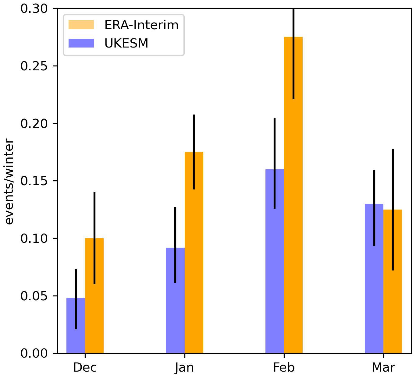
Figure 1 SSWs per NH winter season separated by month within the UKESM piControl and ERA-Interim datasets. Error bars are derived using a bootstrap resampling method in which random selections of 50 years are chosen from the SSW data and the SSW rate recorded to build a PDF of events per season. In total, 10 000 such resamples are carried out, and the 97.5 and 2.5 percentile values are used as error bounds.

The model exhibits variability in SSW frequency comparable to observations, including both hiatus and consecutive SSW intervals. Figure 2 shows a sample 40-year interval of the polar vortex zonal wind strength from the UKESM simulation compared with a similar length from the ERA-Interim reanalysis. An extended interval of mainly westerly anomalies indicating a strengthened vortex and lack of SSWs can be seen towards the end of the 40-year interval, similar to the 1990s in ERA-Interim when only two SSW events were recorded in the decade. The simulation contains eight such hiatus intervals with at least 10 consecutive years with no SSWs, the longest of which lasts 16 years. On the other hand, the simulation only contains two intervals in which 10 consecutive years exhibit at least one SSW. However, if the threshold interval width for identifying hiatus and consecutive SSW intervals is shortened from 10 to 5 years, then nine consecutive SSW intervals and 25 hiatus intervals are found. These statistics indicate that UKESM is not only able to reproduce the mean state characteristics of SSW events but also decadal-scale variations in SSW rate, underlining its suitability for this study.

The second major mode of stratospheric variability is the QBO at equatorial latitudes which is present at all times of the year. Figure 3 shows the equatorial wind time series from a sample 40-year interval of the simulation compared with the ERA-Interim dataset. The mean period of the oscillation is longer than observed, at ∼ 38 months compared to ∼ 28 months in ERA-Interim (Kawatani, 2016). As a result, the vertical shear zones descend less rapidly than observed. There is also a westerly bias at low levels where the QBO-E phase does not extend sufficiently deep into the lower stratosphere, which is a common bias in many models (Bushell et al., 2020). The descending shear zones also appear more regular than observed, but there is nevertheless some evidence of decadal-scale variations, e.g. in the degree of stalling at 30 hPa, although it is not as pronounced as in the observations.

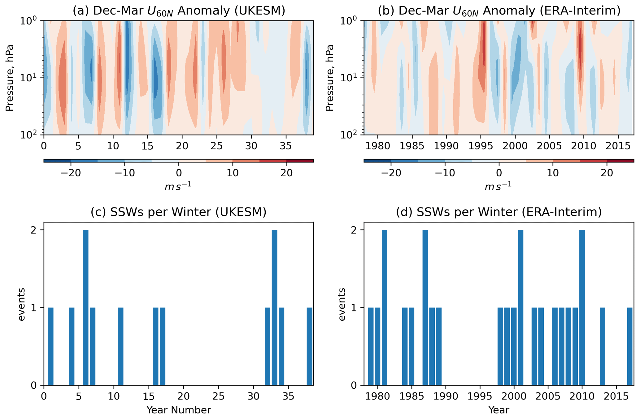
Figure 2 (a, b) December–March annual mean ZMZW anomaly from the climatological mean at 60^∘ N from a 40-year sample from the pre-industrial control simulation of UKESM (a) and the ERA-Interim dataset between 1979 and 2018 (b). (c, d) Time series of SSWs recorded per winter season in the same datasets.

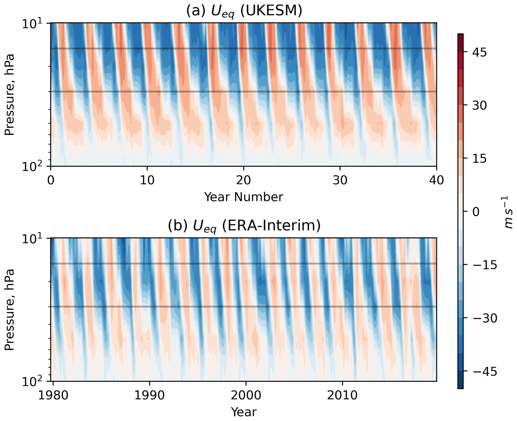
Figure 3 ZMZW averaged between 5^∘ S–5^∘ N latitude from a 40-year sample of the pre-industrial control simulation of UKESM (a) and the ERA-Interim dataset between 1979 and 2018 (b). Horizontal lines mark the 15 and 30 hPa levels between which the deep QBO metric employed by Andrews et al. (2019) is defined.

There is evidence of coupling between the two major modes of stratospheric variability in the model, giving rise to a Holton–Tan relationship (Anstey et al., 2020). Figure 4 shows height–latitude cross sections of NH winter zonal wind differences between QBO-E–QBO-W composites defined at various equatorial levels. The familiar pancake structure of alternating easterly/westerly differences is present at equatorial latitudes, indicative of the QBO phase but there is also a response at high latitudes. In good agreement with observations the largest high-latitude response amplitude is seen when the QBO is defined at 50 hPa, with anomalously weaker polar vortex strength in QBO-E than in QBO-W years. Higher levels (15 and 20 hPa) show little significant QBO–vortex coupling. For comparison, we also show in Fig. 4 the composite different response for QBO composites selected on the basis of the average QBO winds over a greater depth of the equatorial atmosphere (15–30 and 20–50 hPa). We note that while this QBO definition will select some of the same years as in the separate single-level composite definitions, it is specifically designed to identify only QBO phases that have extended vertical coherence, following Gray et al. (2018) and Andrews et al. (2019), so the resulting composite differences in Fig. 4 will not necessarily be an average of the corresponding single-level differences. Interestingly, the 15–30 hPa deep QBO selects years that exhibit not only a weaker polar vortex in QBO-E but also a weaker subtropical tropospheric jet (see 200 hPa, 30–40^∘ N). This results in a more coherent response in the midlatitude troposphere and at the surface, in excellent agreement with the results of Gray et al. (2018) and Andrews et al. (2019).

Figure 4 December–March ZMZW composite differences between QBO east and QBO west phases evaluated in September–October at individual levels as well as using the deep QBO metric. The phase of the QBO is defined as in Fig. 1 – the equatorial September–November ZMZW of greater magnitude than 5 m s⁻¹. Coloured shading indicates differences significant above the 95 % confidence level under a two-tailed Student's t test.

The presence of the Holton–Tan relationship is also seen in the modelled frequency of SSWs (Fig. 5). Significantly higher rates are observed in QBO-E winters than QBO-W. Also notable is the asymmetry in abundance of QBO-E and QBO-W winters – nearly twice as many QBO-E winters are observed compared to QBO-W under all phase definitions (Fig. 5, legends). This suggests an element of phase locking between the QBO and the seasonal cycle possibly associated with seasonally variations in the strength of mean equatorial upwelling or midlatitude planetary wave forcing in winter (Pascoe et al., 2005; Gruzdev and Bezverkhny, 2000; Rajendran et al., 2015), resulting in QBO phase transitions that occur preferentially in certain months.

Figure 5 SSWs per winter season for years exhibiting QBO-E and QBO-W conditions in early winter (September–November) defined on different pressure levels (a, b) as well as using the deep metric (c), the vertical mean between 15 and 30 hPa defined in Andrews et al. (2019). The QBO phase is defined as any September–November equatorial (5^∘ S–5^∘ N average) ZMZW that exceeds a magnitude of 5 m s⁻¹. Error bars on all plots are derived using the same bootstrapping method outlined in Fig. 1.

3.2 Regression analysis

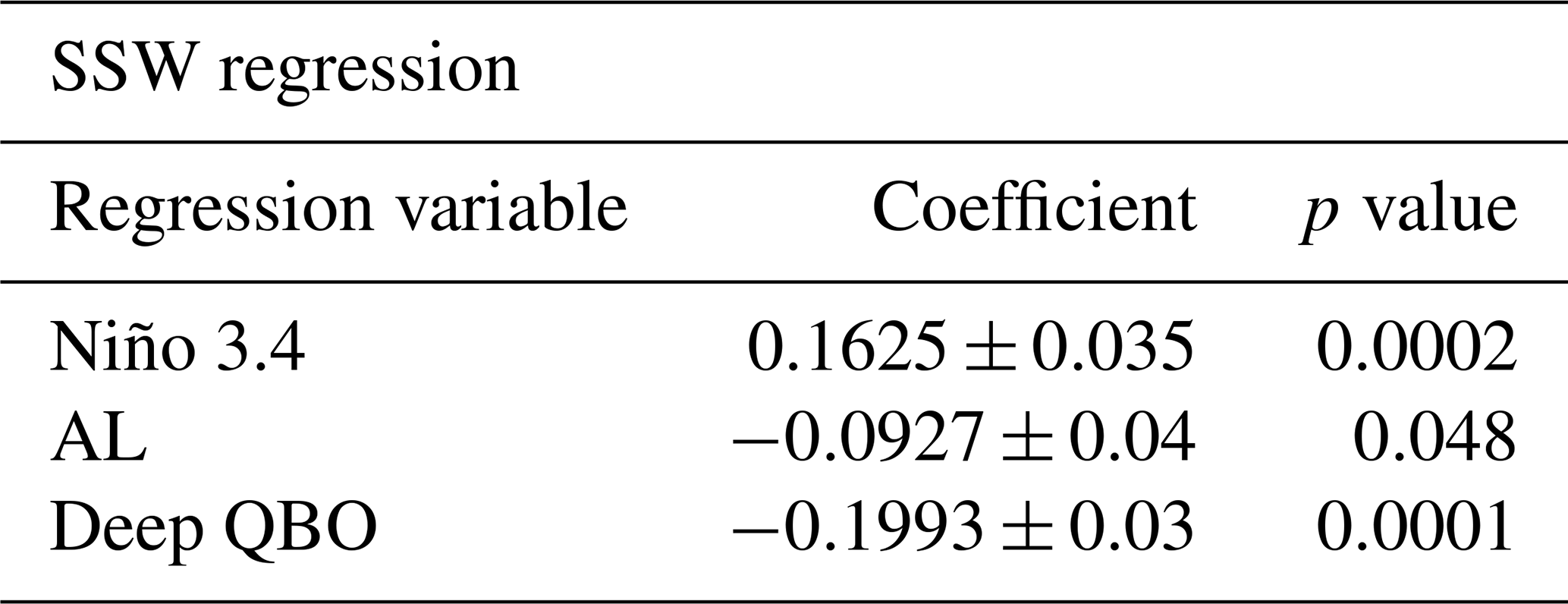
We next employ a multi-linear regression analysis to measure the relative contributions to the time series of SSWs per year (as in Fig. 2) from the QBO, ENSO and AL. The results from this analysis are summarised in Table 1. Sensitivity experiments were performed to identify the optimum averaging intervals (lags) for each index: the deep 15–30 hPa QBO index and Niño 3.4 indices were both defined using early winter (September–November) averages, while the AL index was defined using December–March averages. The coefficients are all significant to the 95 % level but are relatively small, and the R² score is only 0.047, indicating these variables account for only a small portion of the variability in the SSW time series. While results from this multi-linear regression approach are easy to interpret, the approach does not directly tackle the problem posed in this study, that of multi-decadal variability in SSWs and its origins, for two main reasons. Firstly, regression analysis assumes stationarity; i.e. it provides a measure of stationary contributions to variability and will only highlight signals that are relatively persistent for the whole simulation. Secondly, it analyses variability in the time series at all timescales simultaneously, so that the results are dominated by the timescales with larger amplitude variations. This means that the results in Table 1 are most likely dominated by the shorter (interannual) timescales and any small-amplitude variations at longer timescales will not be revealed. The latter can be addressed to some extent by smoothing or filtering the time series, as discussed in the next section, but this requires prior knowledge of which frequencies are of interest. An alternative and superior approach to this problem employs wavelet analysis, described more fully in the next section, which successively examines the frequency intervals to identify the presence of signals, thus avoiding dominance by one particular frequency and also examines the time evolution of the signal so that non-stationary signals can also be identified.

Table 1 Summary of results from regression analysis of SSWs per NH winter time series.

3.3 Long-term variability of the polar vortex

A more comprehensive assessment of the long-term variability of SSWs can be made using a wavelet power spectrum approach. We count the number of SSWs in each winter season (December–March) and calculate the corresponding wavelet power spectrum, shown in Fig. 6. As described above, the analysis highlights the presence of power in the signal as a function of frequency (period in years, along the y axis) and as a function of time (year of simulation along the x axis). As expected, there is an intermittent but relatively persistent signal with the period around 2–4 years throughout the simulation, corresponding to the period of the QBO which supports the presence of a Holton–Tan relationship between the QBO and the polar vortex in the model. The so-called “global power spectrum” (i.e. the time average of the wavelet spectrum) shown on the right of Fig. 6 shows that the signal is on the boundary of the 95 % statistical significance. Other signals at periods near 20–30 years are similarly intermittent and manifest as a peak in the time-averaged spectrum that is also near the 95 % significance boundary. The most persistent feature of the series appears at periods between ∼ 60–90 years in the interval between 400–800 years. This feature shows statistical significance (based on comparisons between power in the spectrum and that of an AR1 process with the same autocorrelation structure as the series being analysed) for around 350 years of the 1000-year simulation but does not cross the significance threshold for the time-averaged spectra. There is a possible limitation of this wavelet methodology due to the discrete nature of the time series being analysed (time points take values 0, 1 and/or 2). The Morlet wavelet is a continuous function, and as a result, convolution with a highly discretised series may alias features on the resulting wavelet spectra. This limitation must be considered when drawing conclusions from the wavelet spectra and is discussed further below.

Figure 6 (a) SSW events per December–March season in UKESM. (c) Wavelet power spectrum of time series in panel (a). Hatching represents area outside the cone of influence in which edge effects are significant and power should not be considered. Yellow contours represent the 95 % confidence level assuming mean background AR1 red noise. (b) Morlet wavelet used for the wavelet transform in the time domain. (d) Global power spectrum, the wavelet power averaged over the whole simulation (blue line) and global 95 % confidence spectrum (dashed red line).

Figure 7 (a) SSW events per December–March season in UKESM smoothed using a 5-year running mean. (c) Wavelet power spectrum of time series in panel (a). Hatching represents area outside the cone of influence in which edge effects are significant and power should not be considered. Yellow contours represent 95 % confidence level assuming mean background AR1 red noise. (b) Morlet wavelet used for the wavelet transform in the time domain. (d) Global power spectrum, the wavelet power averaged over the whole simulation and global 95 % confidence spectrum.

The focus of this study is on the longer-term time variations to understand the source of variability characterised by hiatus intervals (no SSWs over an extended period) and consecutive-event intervals (at least one SSW every year for an extended period). We therefore apply low-pass filtering to the time series of SSWs per season using a 5-year rolling window and examine the spectral characteristics of this smoothed series (which we refer to henceforth as SSW_5 years). This averaging is similar to the standard practice of smoothing daily data to remove the noise associated with daily weather variations, thus isolating longer seasonal timescales. It also decreases the impact of the time series discretisation by reducing the chance of introducing spurious spectral features on the wavelet power spectrum which could be otherwise encountered when analysing the unsmoothed time series.

The wavelet power spectrum of SSW_5 years (Fig. 7) shares many of the characteristics of the spectra of the unsmoothed series (Fig. 6), but the longer period signals are now more clearly evident, as expected. The SSW_5 years wavelet spectrum shows the two broad regions of statistically significant maxima corresponding to signal periods of ∼ 20–30 and ∼ 60–90 years but with increased significance both locally and in the time average. For example, the feature around the 90-year period appears significant for 450 years in SSW_5 years compared to 350 years before smoothing. One possible explanation for this increase lies in our definition of the significance level on power which is dependent on the lag-1 autocorrelation of the time series. Introducing a 5-year averaging window will increase the autocorrelation, possibly leading to a less strict significance level. However, this is unlikely because the significance level is constructed using a red-noise process with the same autocorrelation as the series. This means that for SSW_5 years, the threshold for the 95 % confidence level increases with increasing period more steeply than in the unsmoothed case, and yet the power exhibited at those long periods in SSW_5 years nevertheless achieves higher statistical significance. This indicates that the smoothing has enhanced the visibility of a real signal in the SSW_5 years time series that was less visible in the unsmoothed time series. As a check for robustness, we also include the SSW_5 years wavelet spectrum including November SSW events (Appendix Fig. A1). It looks similar to the spectrum shown in Fig. 7 particularly on ∼ 60- to 90-year timescales with persistent power for around 450 years of the simulation at these periods.

3.4 Surface forcing of polar vortex variability

In the absence of external forcing mechanisms such as greenhouse gas or anthropogenic aerosol forcing, the presence of long-term variability such as the 60- to 90-year periodicity seen in SSW_5 years (Fig. 7) suggests a source of long-term internal variability from within the climate system.

The most obvious potential driver of such long timescale variability is the ocean due to its high degree of thermal inertia. Previous work has identified coupling between tropical SSTs and the polar vortex, such as the relationship to ENSO conditions (see Sect. 1). The model exhibits an expected connection between ENSO and the vortex on interannual timescales indicated by the regression analysis results (Table 1) and ZMZW composites for El Niño and La Niña winters (Fig. A2). Figure 8a shows the wavelet power spectrum for the 5-year smoothed September–November Niño 3.4 index as well as the cross-power spectrum with SSW_5 years. We use the early NH winter ENSO index to capture the lagged response of the vortex to this mode of variability. The ENSO index is slowly varying so will likely remain in the same state between early and mid-winter. We also smooth the ENSO index for the purposes of calculating the cross spectrum with SSW_5 years. (The spectrum of the unsmoothed Niño 3.4 index is provided in Fig. A3 and shows significant power in the expected period range of 4–7 years; Santoso et al., 2017.) The smoothed Niño 3.4 index shows intermittent power at periods around 16 years which appears significant in the global spectrum. It also exhibits a small signal coincident with the 90-year variability in SSW_5 years; however, this feature only persists for around 100 years of the simulation. Cross spectra between the two series (Fig. 8b) reveal that the coincidence in signals at the 90-year period, while significant under our test, is marginally prominent but only covers a small proportion of significant signals in SSW_5 years. This suggests there may be some contribution from ENSO to the observed SSW variability but it is only marginally significant, and on its own it cannot explain the signal in SSW_5 years that persists for 450 years. The source of this ENSO signal at 90-year periods is unclear, although the PDO spectrum shares some of the same characteristics on the 90-year timescale (Fig. A4), which is consistent with results of Newman et al. (2016), who proposed the PDO as a low-pass-filtered version of ENSO.

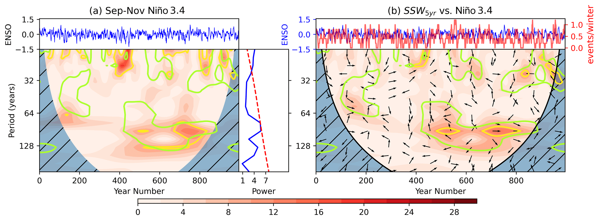
Figure 8 (a) Top: Niño 3.4 time series; bottom left: wavelet power spectrum (shaded contours represent wavelet power and yellow contours the 95 % significance level compared to an AR1 process); bottom right: global wavelet power spectrum (blue) and 95 % confidence level (dashed red). (b) Cross spectra between SSW_5 years and the Niño 3.4 index; top: Niño 3.4 and SSW_5 years time series; bottom: cross-power spectrum. Shading indicates cross power, yellow contours the 95 % confidence interval and arrows the relative phase angle between signals in the time series (to the right: in phase; vertically upwards: $\frac{\mathit{\pi }}{\mathrm{2}}$ out of phase with SSWs leading; to the left: π out of phase; vertically downwards: $\frac{\mathit{\pi }}{\mathrm{2}}$ out of phase Niño 3.4 leading). Green contours on both spectra represent the 95 % confidence intervals for the wavelet power spectrum of SSW_5 years.

In the interest of completeness, we also explore the long-term variability of other tropical ocean regions and their potential teleconnections with the polar vortex. Four additional tropical regions were selected based on those identified by Scaife et al. (2017) and outlined in Sect. 2. While all four regions show some elements of multi-decadal variability (Fig. A5), particularly the tropical Atlantic with a peak period of approximately 140 years for 700 years of the simulation, none of the spectra show variability that coincides well with that of SSW_5 years. There is some overlap of the Atlantic and tropical eastern Pacific spectra with the regions of significant periodicity at around 60–90 years in the SSW_5 years spectrum but, like the Niño 3.4 index, the overlaps and cross power between the series (Figs. A3 and A4) are minimal and cannot reasonably explain the vortex signal, especially the signal of period approximately 90 years that persists in SSW_5 years for around 450 years (Figs. A3 and A4, green contours).

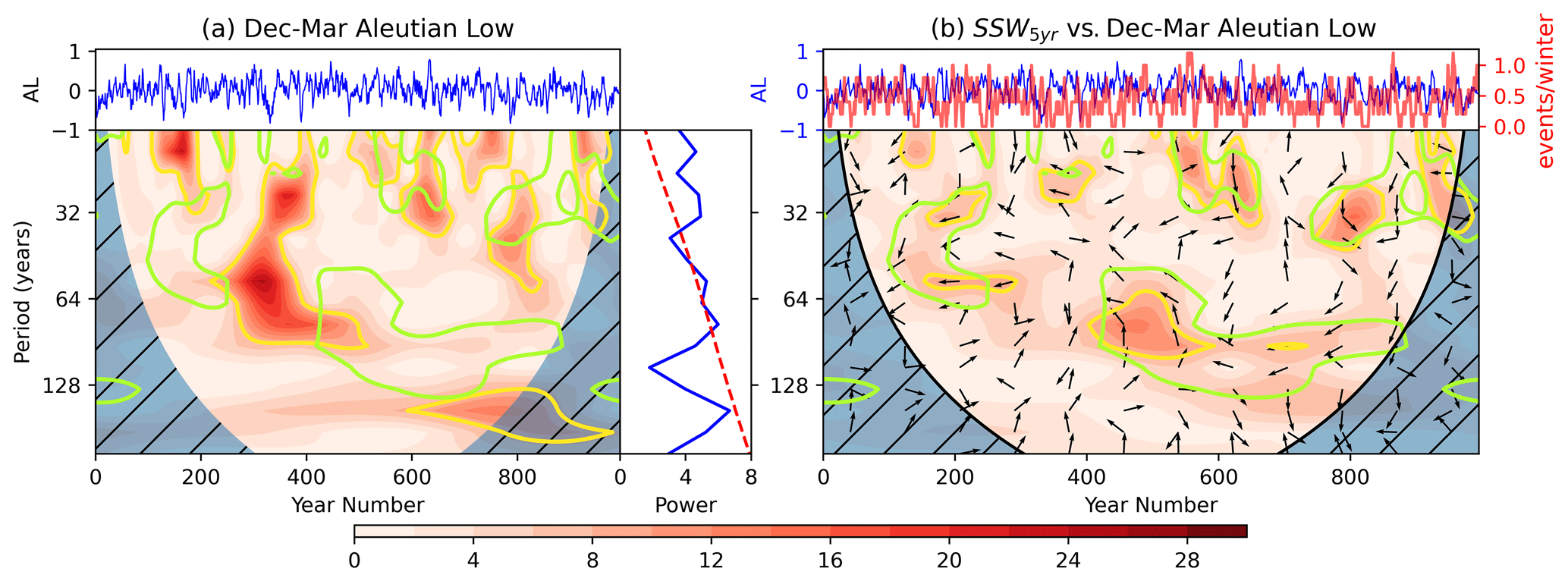
Figure 9 As Fig. 8 for the December–March Aleutian Low index smoothed with a 5-year window. (a) AL time series and associated wavelet power spectrum. (b) Cross-power spectrum between AL and SSW_5 years.

The strength of the AL has also been used as an indicator of tropospheric wave forcing and its influence on the polar vortex (Woo et al., 2015). A similar wavelet and cross-spectrum analysis was therefore performed using an index based on the strength of the modelled NH winter (December–March) AL (see Sect. 2 for details). The wavelet power spectrum for the 5-year smoothed AL index (Fig. 9a) exhibits elements of periodic signals with maximum power corresponding to a period of around 55 years (between 40–60 years) but with fairly minimal overlap with the regions enclosed by the 95 % confidence level in the corresponding SSW wavelet analysis (green contours). AL indices derived from different winter months give similar spectral patterns (not shown). The cross-spectrum analysis between the AL and SSW_5 years (Fig. 9b) highlights this relatively small region of overlap in the interval between years 400–500. However, the phase relationship, indicated by the arrows in that region of overlap, is difficult to interpret. The proposed physical mechanism of coupling between the AL and the vortex (Woo et al., 2015) involves an association between a deeper AL (i.e. lower pressure and hence a negative anomaly) with increased frequency of SSWs. This negative correlation would give rise to arrows pointing to the left if the relationship was present. In contrast, the upward arrows in Fig. 9b indicate a $\frac{\mathit{\pi }}{\mathrm{2}}$ phase difference between the indices on these 60-year timescales, suggesting that peaks in SSW_5 years variations are associated with maximum rates of change of the AL index at the same periods. As with Niño 3.4, the spectra of the AL share some features with those of the PDO (Fig. A4). This is consistent with studies on these modes of variability which find significant correlation of the PDO and AL (Mantua et al., 1997; Rodionov et al., 2005), as well as studies that examine influence of PDO on vortex strength through a pathway involving the AL and ENSO (Rao et al., 2019). Despite this possible pathway, the relatively short time interval of overlap between the AL and SSW_5 years signals at the 60-year period, the absence of any significant signal around the 90-year period, together with the inconsistent phase relationships, points to a conclusion that AL forcing is unlikely to be the primary driver of long-term variability in SSW_5 years. Indeed, examination of the cross spectrum between the unsmoothed AL and SSW indices (Fig. A7) shows little indication of a coherent relationship between the two indices at any timescale. Finally, while the regression results of the unsmoothed indices give a significant coefficient for the AL (Table 1), its magnitude is small compared to that of Niño 3.4 and the deep QBO, the uncertainty on the coefficient is large, and the associated p value is close to the 95 % significance boundary. The weak relationship between the AL and SSWs is unexpected due to the well-acknowledged influence of the AL over planetary wave flux in the upper troposphere (Woo et al., 2015). To attempt to address this, we also analyse an AL metric evaluated as the area-weighted average over a box recommended by Garfinkel et al. (2012), who used an SSW precursor region at 500 hPa height defined by 52.5–72.5^∘ N, 165–195^∘ E. However, we find a lower correlation between this measure and our SSW time series than between the original EOF-based metric and SSWs ($r=-\mathrm{0.21}$ for the EOF-based AL and $r=-\mathrm{0.13}$ for the box-based AL).

3.5 QBO–vortex interactions

Despite some coincident signals between tropical SSTs, AL and SSW_5 years, long-term variability in these surface indices are unable to fully account for the multi-decadal signals in SSW frequency. An additional potential source of internally generated long-term variability may reside within the stratosphere. Studies have noted relatively long-term variations in the strength of the Holton–Tan relationship (Lu et al., 2008, 2014; Osprey et al., 2010), although the cause of these variations is not well understood. In order to investigate this, Fig. 10 shows the wavelet power spectrum of early winter (September–November) QBO winds evaluated at selected levels. Since the QBO evolves relatively slowly, employing September–November averaged winds provides a reasonable representation of the QBO and also allows us to evaluate the in-season lagged relationship between the QBO and subsequent occurrence of an SSW. There is a clear signal between 2 and 4 years for the majority of the simulation, as expected, but no prominent power at longer periods, confirming that there is no significant long-term variability in the periodicity of the QBO winds that could explain the long-term variations in SSW_5 years via the Holton–Tan relationship.

Figure 10 (a–f) September–November mean ZMZW averaged between 5^∘ S–5^∘ N latitude on different pressure levels (a–e) and the deep metric averaged between 15–30 hPa (f). (g–l) Wavelet power spectra for each time series shown in panels (a–c). Shading represents wavelet power with a colour scale the same as that seen in Fig. 6, and yellow contours indicate regions of significant power (> 95 % confidence interval) compared to a background AR1 process.

While the wavelet analysis technique is able to isolate and reveal frequency modulations very well, it is less suited to examine amplitude modulations which are clearly evident in some of the QBO index time series. For example, both the 20 hPa and deep (15–30 hPa) QBO time series show multi-decadal variations in the magnitude of the westerly phase, while the easterly phase amplitudes are relatively uniform in time. Similarly, the 50 and 30 hPa time series show amplitude modulation predominantly in the easterly phase. This amplitude modulation can be highlighted by taking the Hilbert transform of each QBO time series (Fig. 11a–f). Wavelet analysis of the transformed QBO time series now shows significant power on multi-decadal timescales (Fig. 11g–l). In particular, the 20 hPa and deep QBO time series exhibit signals coincident in time and around similar periods (60–90 years) to those observed in SSW_5 years. On the other hand, the QBO indices based on equatorial winds at 50 or 30 hPa show minimal power at these periods, despite showing a strong intraseasonal HT relationship (Fig. 4). Given that the 15–30 hPa deep QBO index exhibits both multi-decadal timescale variability and a strong intraseasonal HT coupling, we continue further analysis of the QBO–SSW interactions using the 15–30 hPa index.

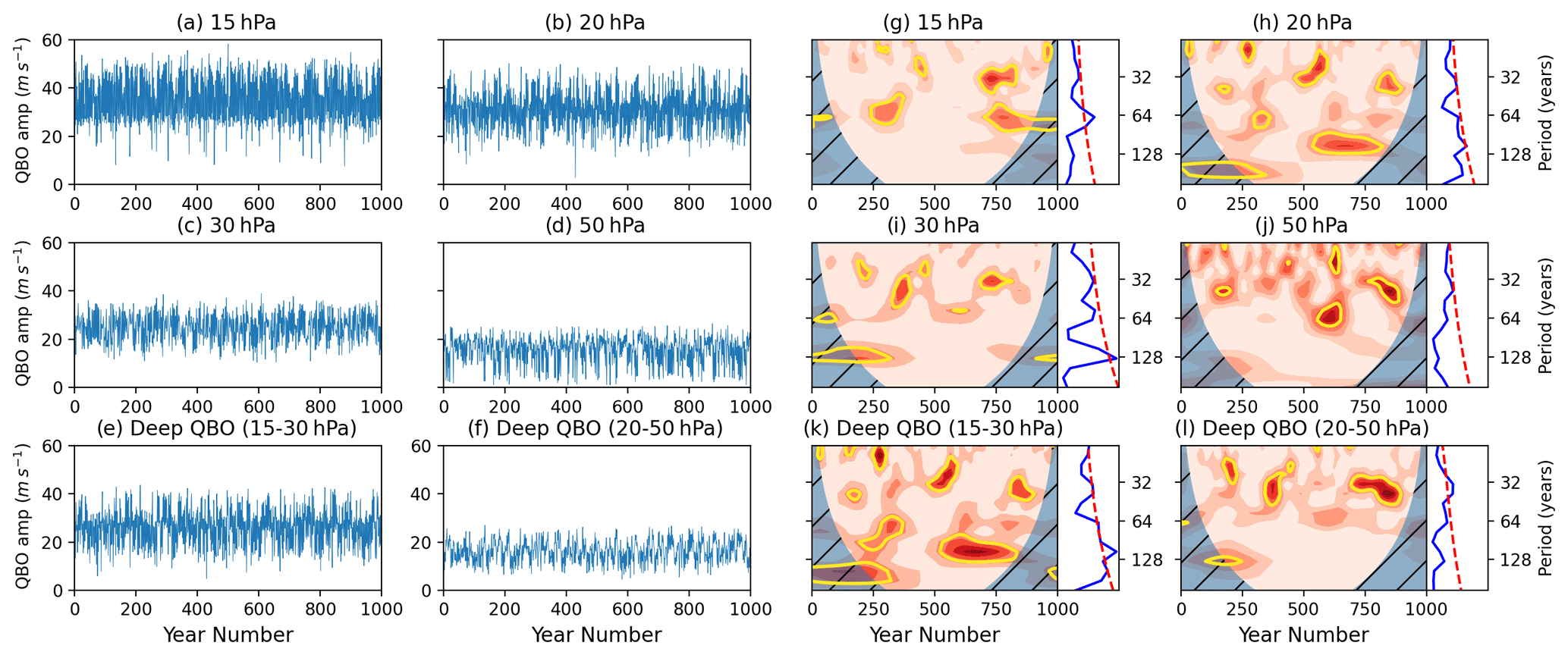
Figure 11 (a–e) Hilbert amplitude of September–November mean ZMZW averaged between 5^∘ S–5^∘ N latitude on different pressure levels (a–e) and the deep metric averaged between 15–30 hPa (f). (g–l) Wavelet power spectra for each time series shown in panels (a–c). Shading represents wavelet power with a colour scale the same as that seen in Fig. 6, and yellow contours indicate regions of significant power (> 95 % confidence interval) compared to a background AR1 process.

Wavelet analysis of the 5-year smoothed deep (15–30 hPa) QBO amplitude modulation index (Fig. 12a) enhances the clarity of the long-term periodicity, showing statistically significant power at around 90 years in the interval between 500–800 years. The cross power between SSW_5 years and this QBO amplitude modulation index (Fig. 12b) coincides extremely well with the signals observed in SSW_5 years at around 90 years. There are also coincident features at other timescales, although the feature between years 450–550 at periods of 60 years is less well captured. The phase relationship arrows in the main region of long-term variability (periods around 90 years in the interval 450–800 years) point broadly to the left (π phase shift), indicating that the signals are approximately anti-phased (the slight downward pointing of the arrows suggests a small deviation from this zero-lag relationship and is discussed below). The anti-phase relationship is consistent with the HT relationship in which a westerly (positive) QBO anomaly corresponds to a reduction in the frequency of SSWs.

Table 2 Summary of results from multi-linear regression analysis of SSW_5 years.

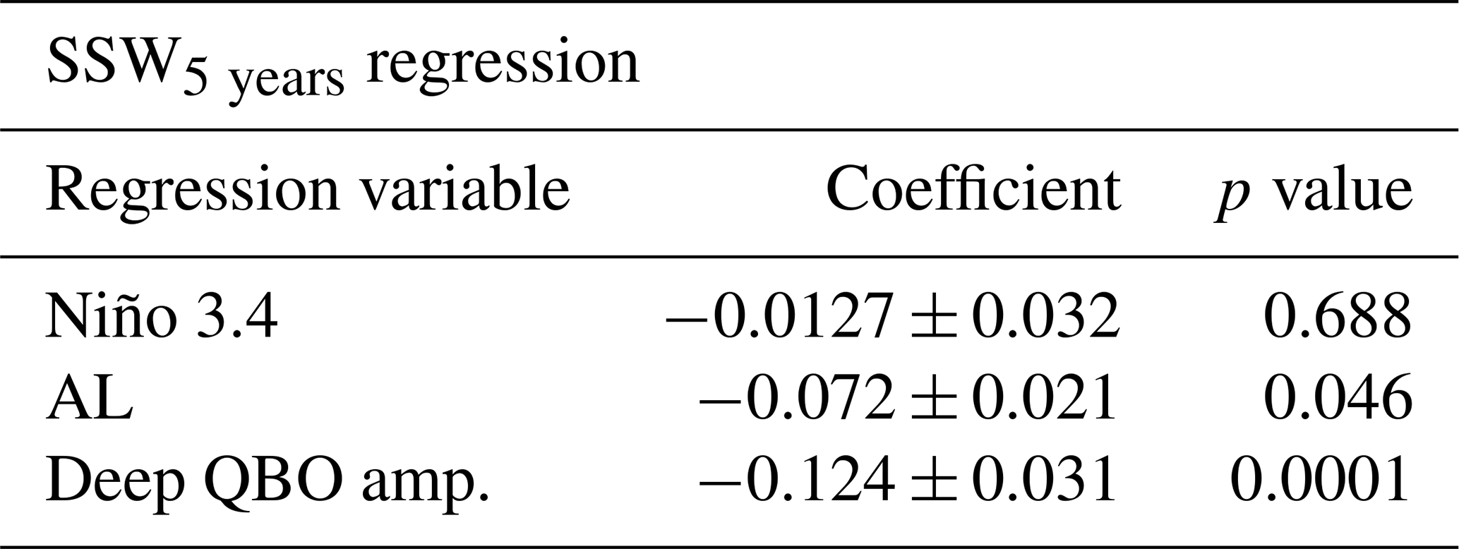
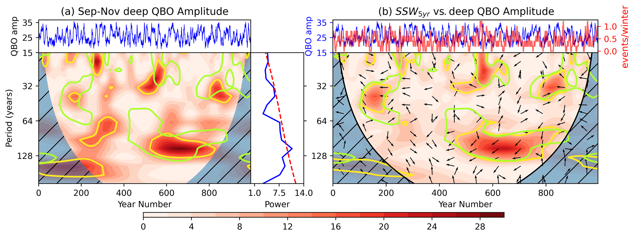
Figure 12 As Fig. 8 for the September–November deep QBO (15–30 hPa) amplitude index smoothed with a 5-year window. (a) QBO amplitude time series and associated wavelet power spectrum. (b) Cross-power spectrum between deep QBO amplitude and SSW_5 years.

In our earlier discussion, we linked long-term variability in SSW frequency to the existence of extended hiatus periods, during which the vortex is relatively undisturbed with no SSW events (Fig. 2). The cross-spectrum analysis with deep QBO amplitude modulation suggests a possible physical interpretation involving the Holton–Tan relationship varying on longer timescales, in which a series of consecutive years that exhibit a large-amplitude deep westerly QBO in early winter leads to a series of winters with reduced SSW frequency, i.e. a hiatus period. Correspondingly, a series of large-amplitude deep easterly QBO years would lead to a series of consecutive-event years.

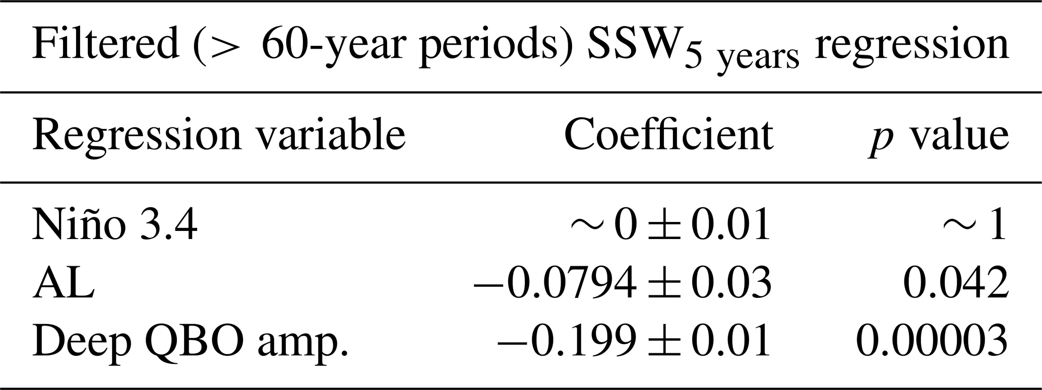
We verify the results of the wavelet analyses described above by repeating the multi-linear regression (Table 1) but using the 5-year smoothed QBO, ENSO and AL indices to measure their relative contributions to the 5-year smoothed SSW_5 years time series. The resulting regression coefficients for the deep QBO amplitude and AL remain significant at the 95 % level, although the AL's contribution remains small and close to the significance boundary. The coefficient for Niño 3.4 is not significant, suggesting that the connection between ENSO and the vortex variability is dominated by timescales of less than 5 years. If we further isolate multi-decadal signals by Fourier filtering each time series, so that only periodicities longer than 60 years are retained, the Niño 3.4 coefficient is near 0, while the deep QBO amplitude signal is near −0.2. This is consistent with our wavelet analysis which suggests a dominant role for QBO amplitude variations on these long timescales. The AL coefficient remains significant but smaller than that of the QBO (and outside error ranges). For completeness, we repeated the regression analysis using a 5-year smoothed PDO index instead of the AL, but there was no significant change in the coefficients (not shown). This is consistent with the fact that the AL and PDO indices exhibit similar spectra, and there is a high correlation between them (−0.45 unfiltered and −0.68 filtered), as also found by Mantua et al. (1997) and Rodionov et al. (2005).

Table 3 Summary of results from multi-linear regression analysis of a Fourier-filtered version of SSW_5 years retaining power corresponding to periods greater than 60 years.

To further clarify the role of the QBO, we note that an examination of Fig. 10 shows that the majority of the long-term amplitude variability in the 15–30 hPa deep QBO index lies in the amplitude of the westerly phase (the easterly phase amplitude is relatively constant with time). Also, as noted earlier, the simulation exhibits more hiatus intervals than consecutive-event intervals, which suggests that the observed long-term variability may arise primarily from the westerly QBO phase. To explore this hypothesis, we isolate the SSW hiatus intervals by modifying the SSW_5 years time series in the following way. All SSW rates above 0.54 events per season (the climatological mean) are reset to 0.54, thereby removing variability in 5-year intervals that exhibit anomalously high SSW rates. Figure 13 shows the cross-power spectrum between this modified SSW_5 years time series and the time series of deep QBO amplitude. It retains significant cross power within the portion of significant SSW_5 years power (green contours in Fig. 13) when compared with Fig. 12b, in which the full time series is used, and also shows a phase relationship significantly closer to anti-phased (i.e. pointing to the left). This is further support that the deep QBO–SSW relationship on these long timescales in the model arises primarily from the SSW hiatus periods.

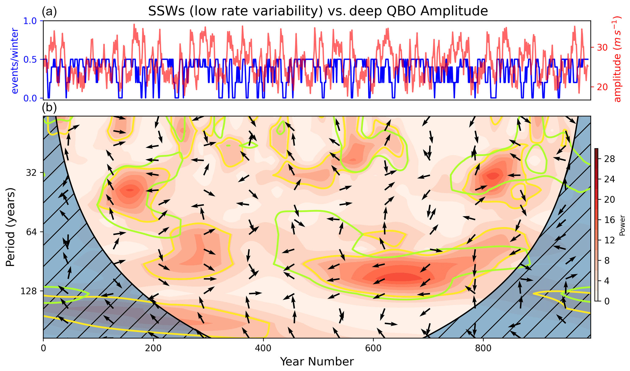
Figure 13 (a) SSW_5 years time series with variability in high SSW rate intervals removed by setting all rates above the climatological mean (0.54 events per season) to the mean (blue) and September–November deep QBO Hilbert amplitude index smoothed with a 5-year window (red). (b) Cross-wavelet power spectrum between the two time series.

An obvious question is whether this sensitivity to deep QBO westerlies that we find in the model is also present in the real atmosphere. Examination of the ERA-Interim dataset shows limited support. Some winters in the 1990s are characterised by anomalously westerly September–November equatorial winds which are vertically coherent between the 15 and 30 hPa levels. However, this effect is intermittent and does not span the whole interval of the 1990s during which SSWs were markedly absent in the observational record (not shown). On the other hand, a mini hiatus that was present in the mid-2010s is associated with 3 years of deep westerly anomaly in the QBO. Overall, it is clear that the relationship, if present in the real atmosphere, is likely obscured by other factors including greenhouse gas increases and volcanic eruptions, and the observational dataset is too short to provide useful validation for these long timescale variations.

4 Summary and discussion

In this study, we have examined variability in the appearance of hiatus and intervals of consecutive SSWs in a 1000-year pre-industrial control simulation of the UK Earth System Model. While there is much observational evidence for an impact of SSWs on the underlying tropospheric weather and climate, their multi-decadal variability and the associated forcing mechanisms are not well understood due to the short observational record. Analysis of long climate model simulations is currently the only available tool for understanding this variability.

We found realistic decadal and multi-decadal variability in the model, with hiatus intervals of 10 years or more in which no SSWs occurred, similar to the observed SSW record in the 1990s (Pawson and Naujokat, 1999; Shindell et al., 1999) and also intervals of consecutive-event periods in which at least one SSW occurred every year, as observed in the early 2000s (Manney et al., 2005). A 5-year smoothed representation of SSW frequency (SSW_5 years) was found to vary periodically for approximately 450 years of the 1000-year simulation with maxima in wavelet power corresponding to periodicity of around 60–90 years.

A possible tropical SST source of this long-term variability was investigated. Wavelet and cross-spectrum analyses were performed using a variety of different tropical SST indices, including the Niño 3.4 index, and also an index of the strength of the AL which is linked to large-scale planetary wave forcing of the winter stratosphere. While all of these indices displayed long-term variability, some of which overlapped with the periodicity and time intervals seen in the SSW_5 years spectrum, none of them could fully account for the extended 450-year interval of significant power at 60–90 years seen in the SSW_5 years spectrum. The weak relationship between the AL and SSW occurrence is unexpected, and modifying the metric by using a box-averaged SLP measure utilised in Garfinkel et al. (2012) did not recover a stronger connection. Further analysis of the AL–SSW relationship in the simulation would be useful (but outside the scope of this study) to explore whether the AL exhibits a connection with the mean vortex strength even though there is no apparent connection with SSW occurrence.

A second possible source of long-term variability involving variations in the QBO was also investigated. A range of QBO indices was considered, including the standard approach of using equatorial winds at a specified pressure level, e.g. 50 hPa, and also a “deep QBO” index which takes the average QBO wind over 15–30 hPa, designed to capture the degree of vertical coherence in the QBO winds (following Gray et al., 2018 and Andrews et al., 2019). A straightforward wavelet analysis of these QBO indices reveals no power at periodicity longer than 2–4 years. However, while there is evidently no long-term variability in the frequency of the QBO, visual examination of the QBO time series clearly shows the presence of long-term variability in the QBO amplitudes. A measure of this amplitude modulation was extracted by taking the Hilbert transform of the QBO index. Wavelet analysis of the amplitude variations from the Hilbert transform of the QBO indices showed long-term periodicity matching that seen in the SSW_5 years wavelet analysis. In particular, the deep QBO index exhibited significant signals coincident with those in SSW_5 years corresponding to periodicities of around 90 years. This overlap accounted for nearly all 450 years of SSW variability present on the 90-year timescale. Regression analysis of 5-year smoothed and filtered indices confirmed the contribution of the deep QBO amplitude to variability in SSWs on timescales greater than 60 years.

Our analysis has therefore revealed an unexpected relationship between the strength and vertical coherence of the QBO and long-term variability in the frequency of SSWs. The relationship was found to be particularly sensitive to the QBO westerly phase. Extended periods of deep westerly QBO phases were associated with hiatus periods with few or no SSWs, consistent with the Holton–Tan relationship. While this result appears compelling, it should be noted that the model showed some biases in its QBO associated with the period and descent rate of shear zones. The extended period of close to 3 years could introduce an element of phase locking between the QBO and seasonal cycle causing winter months to occur preferentially in one QBO phase over the other (evident from the legends in Fig. 5). This may influence QBO–vortex coupling. However, these biases are common in modern GCMs (Bushell et al., 2020), and Rao et al. (2020) show UKESM's representation of the HT effect is better than most major GCMs submitted to CMIP6, indicating this piControl remains one of the most effective tools for studying multi-decadal variability in the stratosphere. Recent work has also shown a large degree of inter-model variability exists in representations of the QBO as well as SSWs (Bushell et al., 2020; Ayarzagüena et al., 2020), so it is possible the result from this study is model dependant. Additional analysis of long simulations from different models is required to verify these results.

Combining the results of all these analyses, our overall conclusion is that multi-decadal variability in SSW frequency in UKESM is primarily accounted for by long-term variability in QBO–SSW coupling, particularly at periodicities of around 90 years and, to a lesser extent, by variability in the intensity of the Aleutian Low at periodicities around 60 years, although coherence with the AL signals is far less persistent than with the QBO. Given the observed impact of SSWs on the underlying tropospheric weather and climate, improved understanding of the source and mechanisms of long-term variability in QBO–SSW interactions is likely to help improve future seasonal weather forecasts and decadal-scale climate predictions. The precise nature of QBO–SSW interaction mechanisms is still not fully understood (Anstey and Shepherd, 2014). While the importance of wave–mean flow interactions is widely recognised, further studies are required to explore the relevance and usefulness of the deep QBO index highlighted in this study, which identifies a vertically coherent QBO phase. It appears to be especially relevant to long-term QBO–SSW interactions during the QBO-W phase.

Further exploration of the source of the long-term variability in amplitude of the QBO-W phase is also required. While a direct influence of tropical SSTs on long-term variability in SSW frequency has not been supported by this study, there may nevertheless be an important teleconnection via the QBO in which the SSTs influence the QBO which subsequently influences the SSW frequency via the Holton–Tan relationship. Initial investigation through cross-spectrum analysis of the deep QBO index with ENSO and selected SST indices shows some contribution from each of the regions (Figs. A6 and A7), not surprisingly because of the tropical source of equatorial waves that are known to drive the QBO. A closer examination of the precise nature of forcing of the QBO-W phase in the model, in terms of Kelvin and gravity wave forcing, would be helpful (but outside the scope of this study).

Time series analyses such as those presented here can highlight associations between modes of variability but are less able to determine causality. Where possible, we have selected indices that confirm well-known in-season causality, such as an early winter QBO index compared with a mid-winter SSW index, but determining causality on longer timescales is difficult and would require well-designed climate model experiments. The climate system is extremely complex, with many different interactions between modes of variability. The climate system is also clearly non-stationary, as evident in our simulation where the QBO–SSW interaction shows power at periodicities of 60–90 years for 450 years but is absent in the early half of the simulation. While this complexity means that it is extremely challenging to disentangle the influences or to attribute causality, improved understanding of individual links in this complex system, such as the relationship between the QBO and SSWs, will nevertheless contribute to improved understanding of the whole complex system.

Appendix A

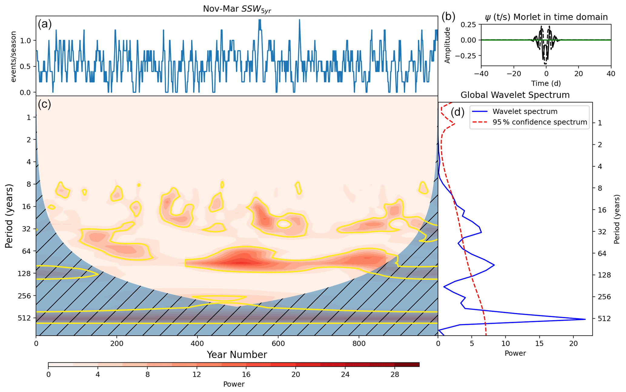
Figure A1 (a) SSW events per November–March season in UKESM smoothed using a 5-year running mean. (c) Wavelet power spectrum of time series in panel (a). Hatching represents area outside the cone of influence in which edge effects are significant and power should not be considered. Yellow contours represent 95 % confidence level assuming mean background AR1 red noise. (b) Morlet wavelet used for the wavelet transform in the time domain. (d) Global power spectrum, the wavelet power averaged over the whole simulation and global 95 % confidence spectrum.

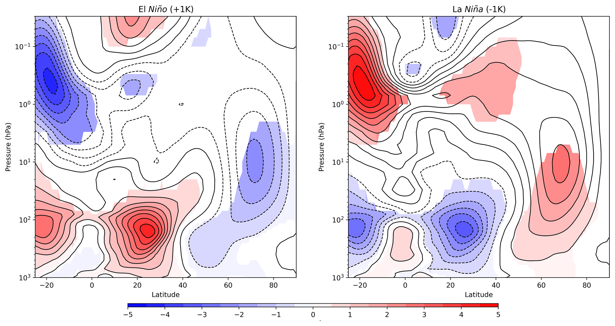
Figure A2 December–March ZMZW anomaly composites for positive (El Niño) and negative (La Niña) phases of the Niño 3.4 index evaluated in September–November. The phase of Niño 3.4 is defined as an SST anomaly of greater magnitude than 1 K. Coloured shading indicates anomalies significant above the 95 % confidence level under a two-tailed Student's t test.

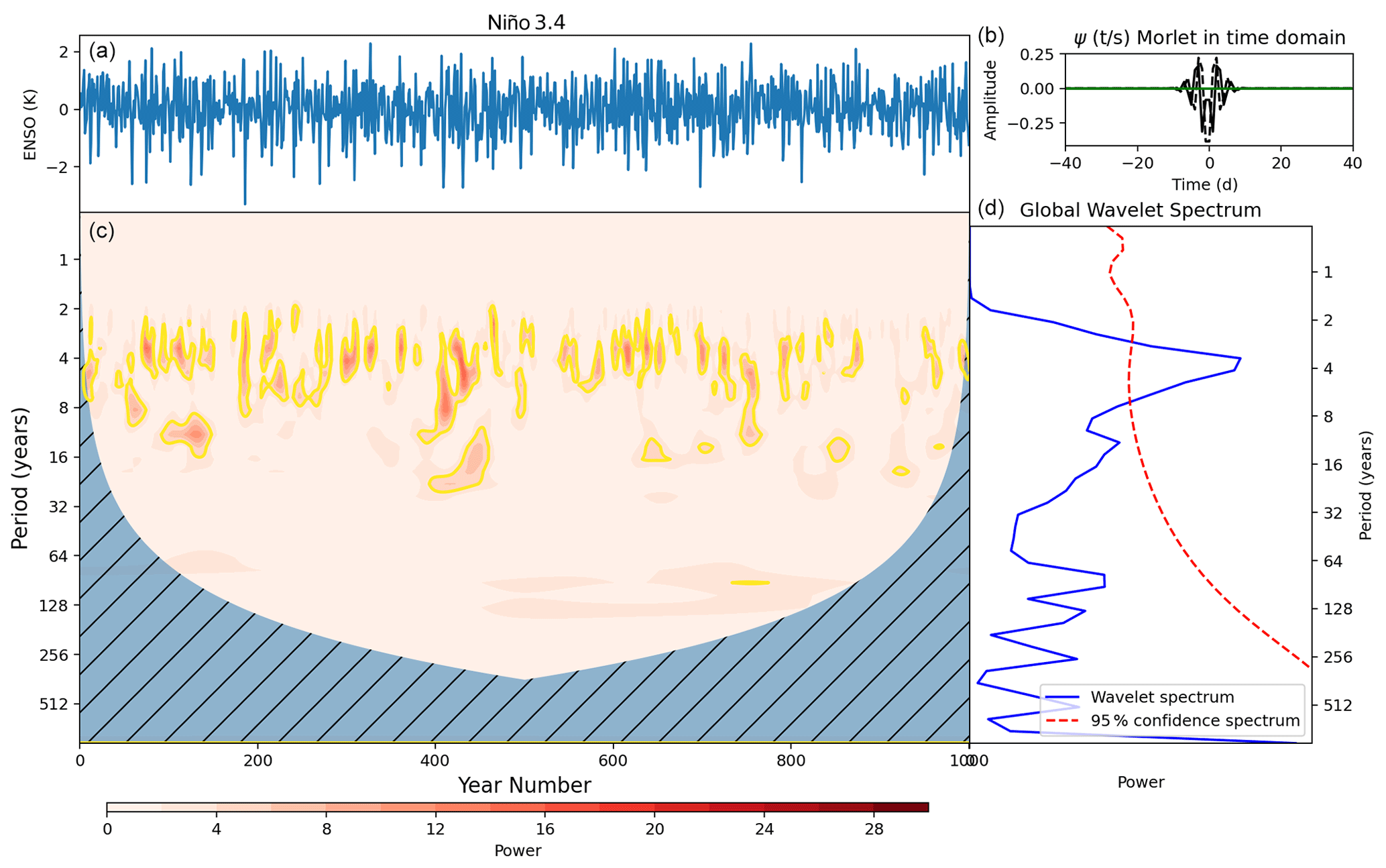
Figure A3 (a) September–November Niño 3.4 index from the UKESM piControl simulation. (c) Wavelet power spectrum of time series in panel (a). Hatching represents area outside the cone of influence in which edge effects are significant and power should not be considered. Yellow contours represent the 95 % confidence level assuming mean background AR1 red noise. (b) Morlet wavelet used for the wavelet transform in the time domain. (d) Global power spectrum, the wavelet power averaged over the whole simulation and global 95 % confidence spectrum.

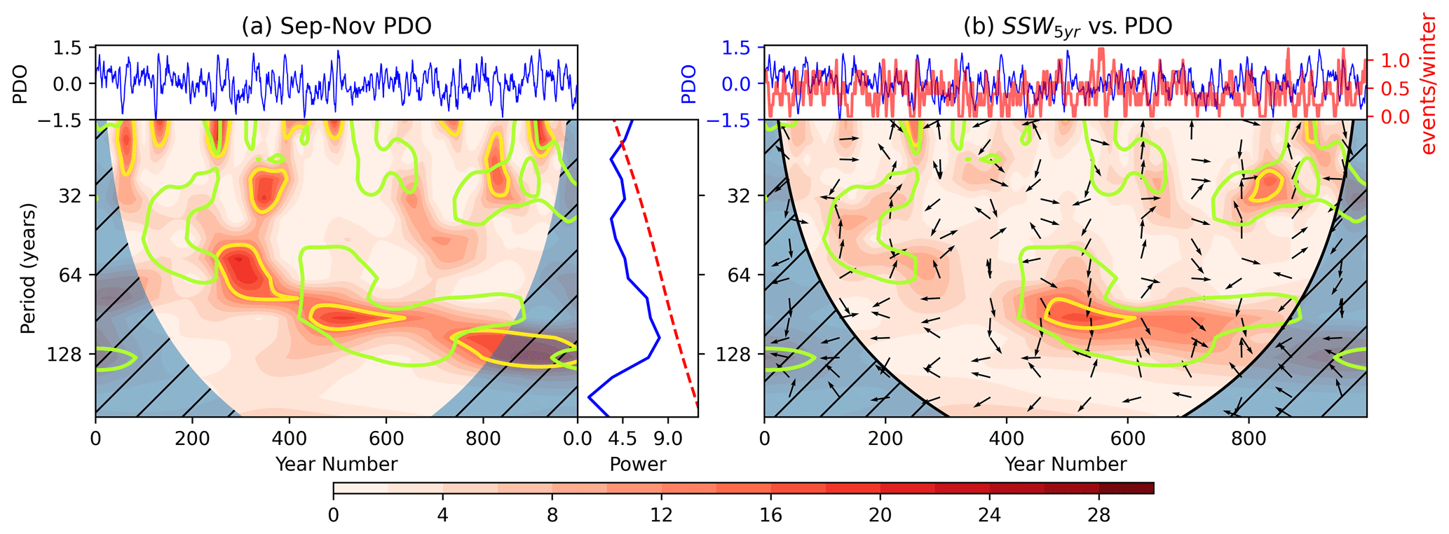
Figure A4 (a) Top: September–November PDO time series; bottom left: wavelet power spectrum (shaded contours represent wavelet power and yellow contours the 95 % significance level compared to an AR1 process); bottom right: global wavelet power spectrum (blue) and 95 % confidence level (dashed red). (b) Cross spectra between SSW_5 years and the PDO index. Top: PDO and SSW_5 years time series; bottom: cross-power spectrum. Shading indicates cross power, yellow contours the 95 % confidence interval and arrows the relative phase angle between signals in the time series. Green contours on both spectra represent the 95 % confidence intervals for the wavelet power spectrum of SSW_5 years.

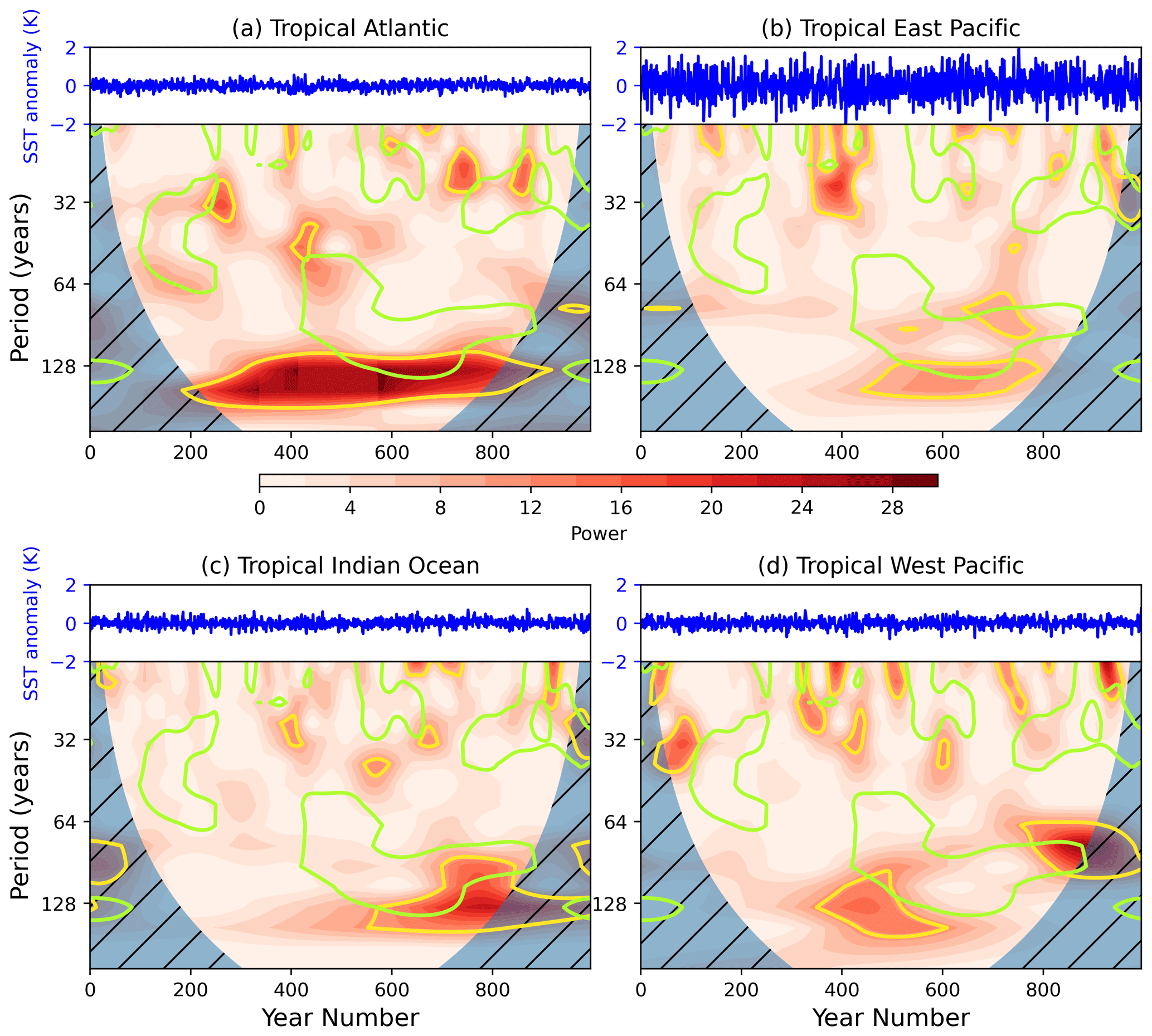
Figure A5 September–November SST anomaly time series and associated wavelet power spectrum for the tropical Atlantic (5^∘ S–5^∘ N, 60^∘ W–0^∘), tropical eastern Pacific (5^∘ S–1^∘ N, 160–270^∘ E), tropical western Pacific (5^∘ S–25^∘ N, 110–140^∘ E) and tropical Indian Ocean (5^∘ S–10^∘ N, 45–100^∘ E). Shading indicates wavelet power, yellow contours show the 95 % confidence level when the power is compared to and AR1 red-noise process, and green contours indicate the 95 % confidence level for the power spectrum of SSW_5 years.

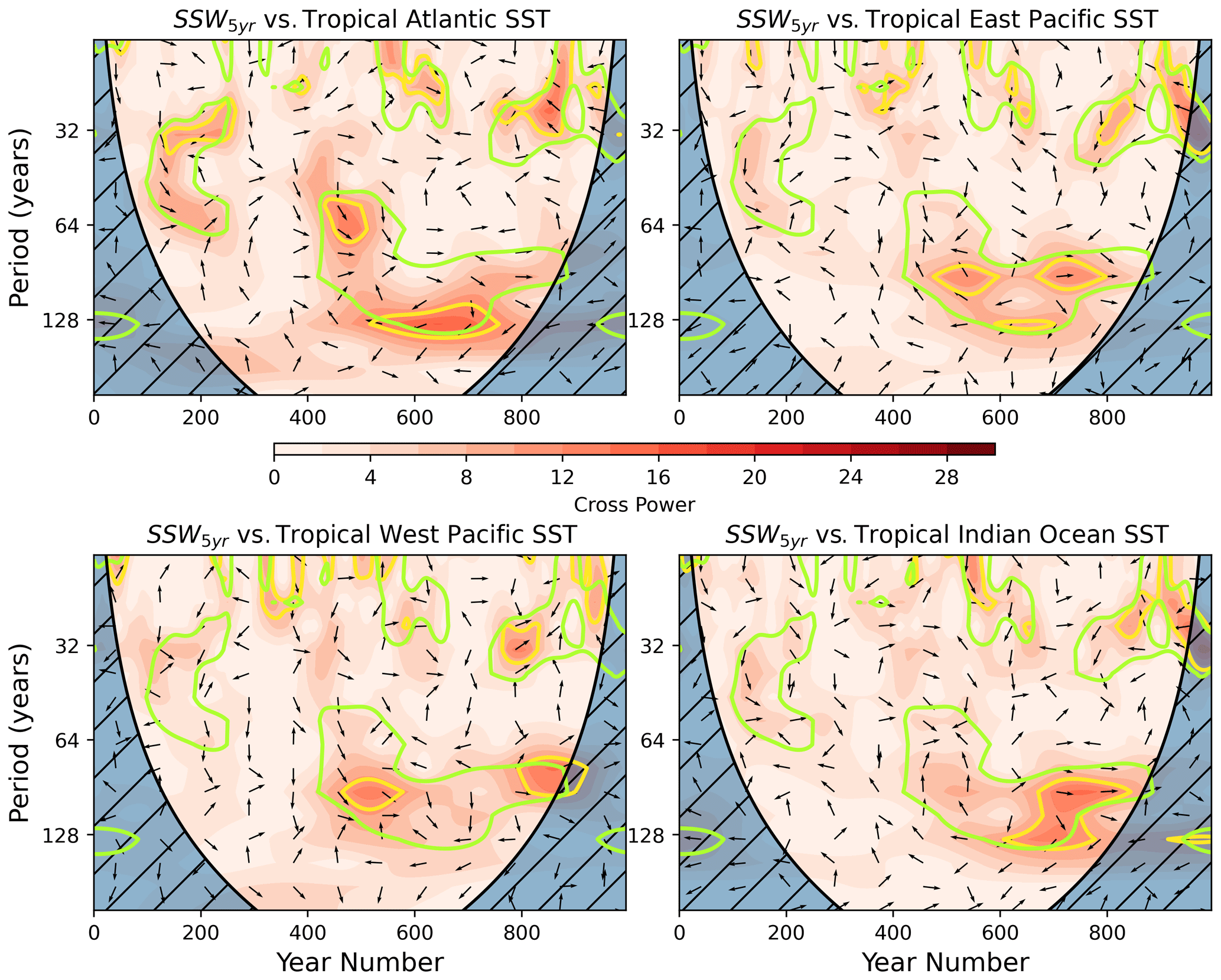
Figure A6 Cross-power spectra between September–November tropical SST anomaly time series and SSW_5 years. SST regions are defined as the tropical Atlantic (5^∘ S–5^∘ N, 60–0^∘ W), tropical eastern Pacific (5^∘ S–1^∘ N, 160–270^∘ E), tropical western Pacific (5^∘ S–25^∘ N, 110–140^∘ E) and tropical Indian Ocean (5^∘ S–10^∘ N, 45–100^∘ E).

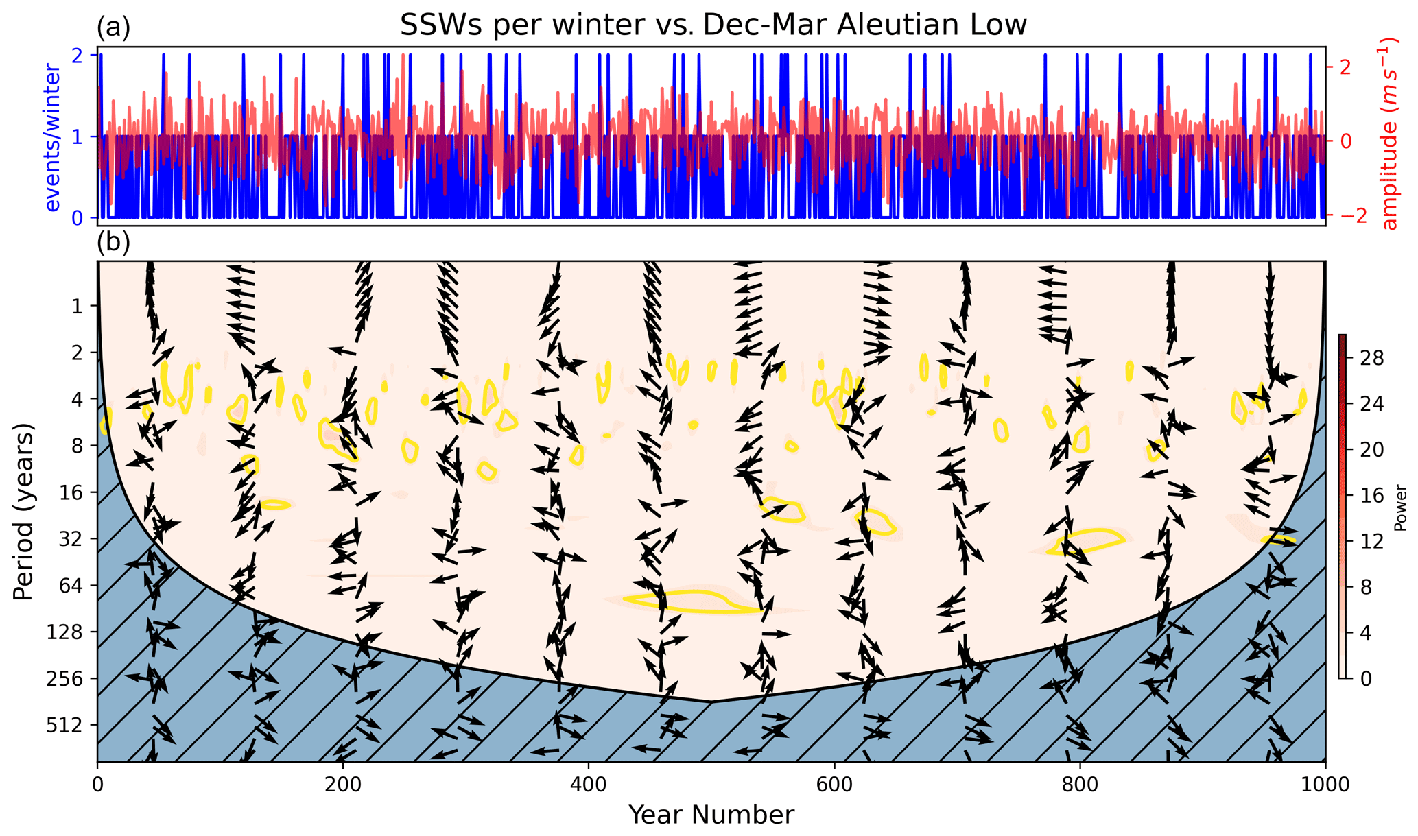
Figure A7 (a) December–March Aleutian Low index (red) and SSWs per NH winter (blue) time series. (b) Cross-wavelet power spectrum between the two time series.

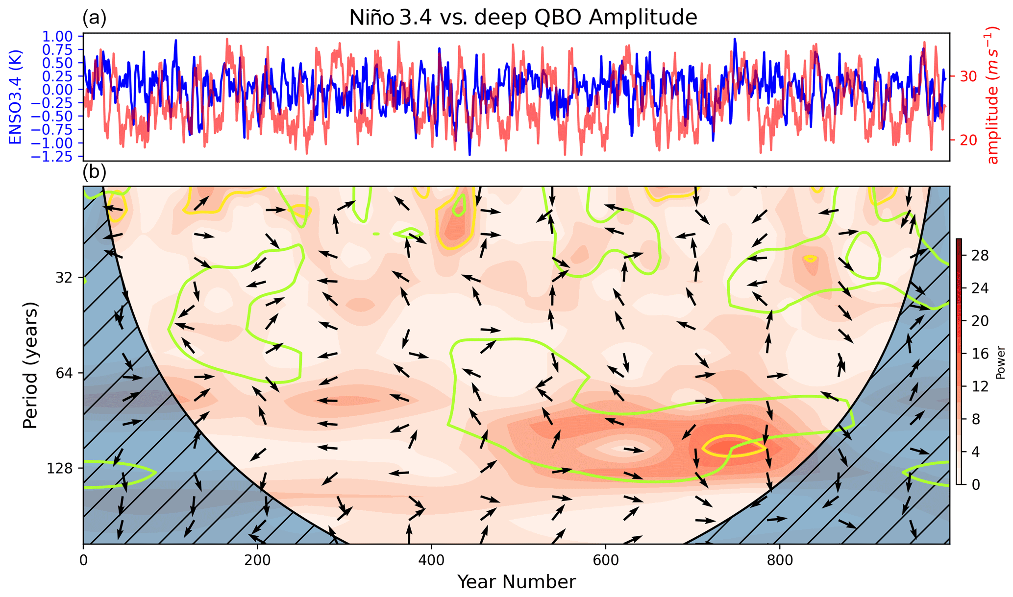
Figure A8 (a) September–November Niño 3.4 index mean (blue) and September–November deep QBO Hilbert amplitude index smoothed with a 5-year window (red). (b) Cross-wavelet power spectrum between the two time series.

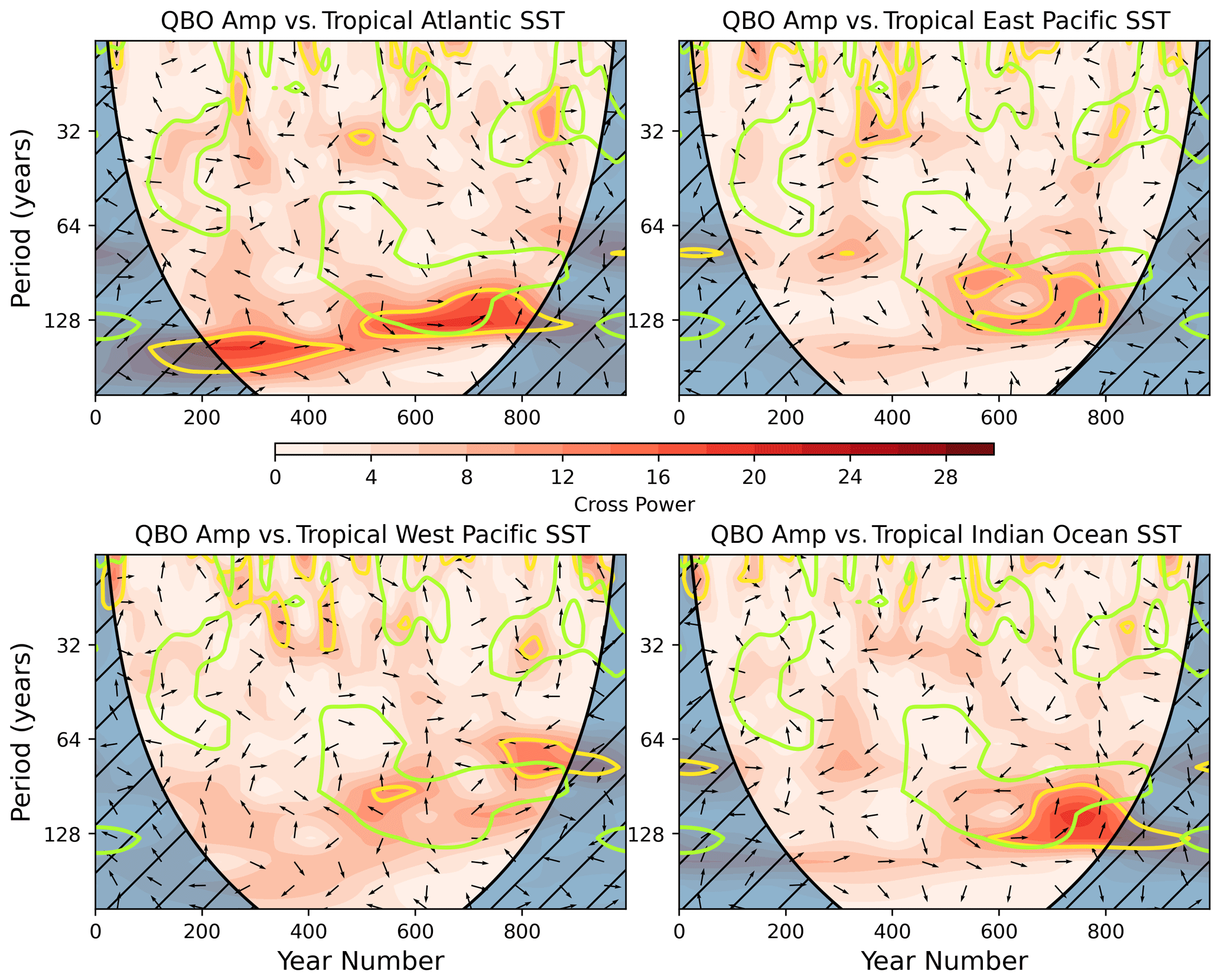
Figure A9 Cross-wavelet power spectra between September–November deep QBO amplitude modulation and September–November SST anomaly in each tropical basin.