the Creative Commons Attribution 4.0 License.
the Creative Commons Attribution 4.0 License.
 | 14 Apr 2021
The role of air–sea fluxes for the water vapour isotope signals in the cold and warm sectors of extratropical cyclones over the Southern Ocean
Katharina Hartmuth
Lukas Jansing
Josué Gehring
Maxi Boettcher
Irina Gorodetskaya
Martin Werner
Heini Wernli
Franziska Aemisegger
Meridional atmospheric transport is an important process in the climate system and has implications for the availability of heat and moisture at high latitudes. Near-surface cold and warm temperature advection over the ocean in the context of extratropical cyclones additionally leads to important air–sea exchange. In this paper, we investigate the impact of these air–sea fluxes on the stable water isotope (SWI) composition of water vapour in the Southern Ocean's atmospheric boundary layer. SWIs serve as a tool to trace phase change processes involved in the atmospheric water cycle and, thus, provide important insight into moist atmospheric processes associated with extratropical cyclones. Here we combine a 3-month ship-based SWI measurement data set around Antarctica with a series of regional high-resolution numerical model simulations from the isotope-enabled numerical weather prediction model COSMOiso. We objectively identify atmospheric cold and warm temperature advection associated with the cold and warm sector of extratropical cyclones, respectively, based on the air–sea temperature difference applied to the measurement and the simulation data sets. A Lagrangian composite analysis of temperature advection based on the COSMOiso simulation data is compiled to identify the main processes affecting the observed variability of the isotopic signal in marine boundary layer water vapour in the region from 35 to 70∘ S. This analysis shows that the cold and warm sectors of extratropical cyclones are associated with contrasting SWI signals. Specifically, the measurements show that the median values of δ18O and δ2H in the atmospheric water vapour are 3.8 ‰ and 27.9 ‰ higher during warm than during cold advection. The median value of the second-order isotope variable deuterium excess d, which can be used as a measure of non-equilibrium processes during phase changes, is 6.4 ‰ lower during warm than during cold advection. These characteristic isotope signals during cold and warm advection reflect the opposite air–sea fluxes associated with these large-scale transport events. The trajectory-based analysis reveals that the SWI signals in the cold sector are mainly shaped by ocean evaporation. In the warm sector, the air masses experience a net loss of moisture due to dew deposition as they are advected over the relatively colder ocean, which leads to the observed low d. We show that additionally the formation of clouds and precipitation in moist adiabatically ascending warm air parcels can decrease d in boundary layer water vapour. These findings illustrate the highly variable isotopic composition in water vapour due to contrasting air–sea interactions during cold and warm advection, respectively, induced by the circulation associated with extratropical cyclones. SWIs can thus potentially be useful as tracers for meridional air advection and other characteristics associated with the dynamics of the storm tracks over interannual timescales.
- Article
(11786 KB) - Full-text XML
-
Supplement
(1724 KB) - BibTeX
- EndNote


Ocean evaporation is the most important source of atmospheric water vapour and impacts atmospheric and ocean dynamics. In the extratropics and polar regions, strong ocean evaporation can lead to the intensification of extratropical cyclones (e.g. Yau and Jean, 1989; Uotila et al., 2011; Kuwano-Yoshida and Minobe, 2016) and polar lows (Rasmussen and Turner, 2003) and to changes in atmospheric (Neiman et al., 1990; Sinclair et al., 2010) and ocean static stability, for example in cyclone-induced cold ocean wakes (Chen et al., 2010) or by inducing deep water formation at high latitudes (Condron et al., 2006; Condron and Renfrew, 2013). The strength of ocean evaporation in the extratropics is strongly modulated by the large-scale atmospheric flow. Ocean evaporation averaged across extratropical cyclones is similar to the ocean evaporation in the North Atlantic (Rudeva and Gulev, 2010) and the Southern Ocean (Papritz et al., 2014). But there are large differences in ocean evaporation between the cold and warm sectors of extratropical cyclones, which are regions within cyclones of equatorward and poleward air mass transport, respectively. The equatorward advection of dry and cold air in the cold sector of extratropical cyclones leads to a large air–sea moisture gradient and strong large-scale ocean evaporation (Bond and Fleagle, 1988; Boutle et al., 2010; Aemisegger and Papritz, 2018), while weak ocean evaporation or even moisture fluxes from the atmosphere to the ocean, i.e. dew deposition, are observed ahead of the cold front in the warm sector (Fleagle and Nuss, 1985; Persson et al., 2005; Bharti et al., 2019). In polar regions close to the sea ice edge, cyclones induce the advection of cold and dry air over the open ocean, leading to cold air outbreaks and strong ocean evaporation (Papritz et al., 2015). Thus, the large-scale meridional advection modulates air–sea interactions, especially in the storm track regions.
The opposite direction of surface fluxes in the cold and warm sector of extratropical cyclones impact the marine boundary layer (MBL) stability and moisture budget. In the cold sector, positive sensible heat fluxes lead to a low atmospheric stability and a high MBL height (Beare, 2007; Sinclair et al., 2010). In idealised model simulations, the strongest ocean evaporation is seen directly behind the cold front in the region of subsiding dry air (Boutle et al., 2010). Dew deposition on the ocean surface has been observed ahead of the cold front (Persson et al., 2005) and in warm sectors during the passage of extratropical cyclones over cold ocean regions (Neiman et al., 1990). Negative sensible heat fluxes in the warm sector lead to a high boundary layer stability and shallow MBLs (Beare, 2007; Sinclair et al., 2010). The net freshwater flux between the ocean and atmosphere is the sum of ocean evaporation and precipitation. In the warm sector, important precipitation occurs in the region of the warm conveyor belt – a moist, coherent, ascending airstream in front of the cold front (Browning, 1990; Madonna et al., 2014; Pfahl et al., 2014). Frontal precipitation, often related to the warm conveyor belt, can affect the surface moisture fluxes in both sectors of extratropical cyclones (Catto et al., 2012).
The characteristic surface freshwater fluxes in the cold and warm sector of extratropical cyclones are schematically summarised in Fig. 1. Air–sea moisture fluxes in the form of ocean evaporation and dew deposition are caused by a thermodynamic disequilibrium between the ocean and atmosphere, which can be expressed by the relative humidity with respect to sea surface temperature , where qa is the specific humidity of the atmosphere and qs(SST) the saturation specific humidity at sea surface temperature (SST). qs is temperature-dependent and increases with increasing temperature. In the cold sector, where dry and cold air is advected over a relatively warm ocean surface, the air–sea temperature difference (where Ta denotes the air temperature) is negative and hs is low due to a low qa and a relatively high qs. Therefore, the air in the cold sector is generally undersaturated with respect to the ocean, and thus (intense) ocean evaporation is expected (Fig. 1a). Negative surface freshwater fluxes can be observed in the cold sector due to precipitation. The horizontal advection in the cold sector of extratropical cyclones is referred to as cold temperature advection in the following. In contrast, in the warm sector, warm air is advected over a relatively colder ocean surface (referred to as warm temperature advection in the following). Under these environmental conditions, ΔTao is positive and hs is high due to a high qa relative to qs. Therefore, the near-surface air in the warm sector can be close to saturation or oversaturated with respect to the potentially cold ocean surface, leading to weak ocean evaporation or dew deposition (Fig. 1b). Furthermore, precipitation associated with the warm conveyor belt leads to moisture fluxes from the atmosphere to the ocean.
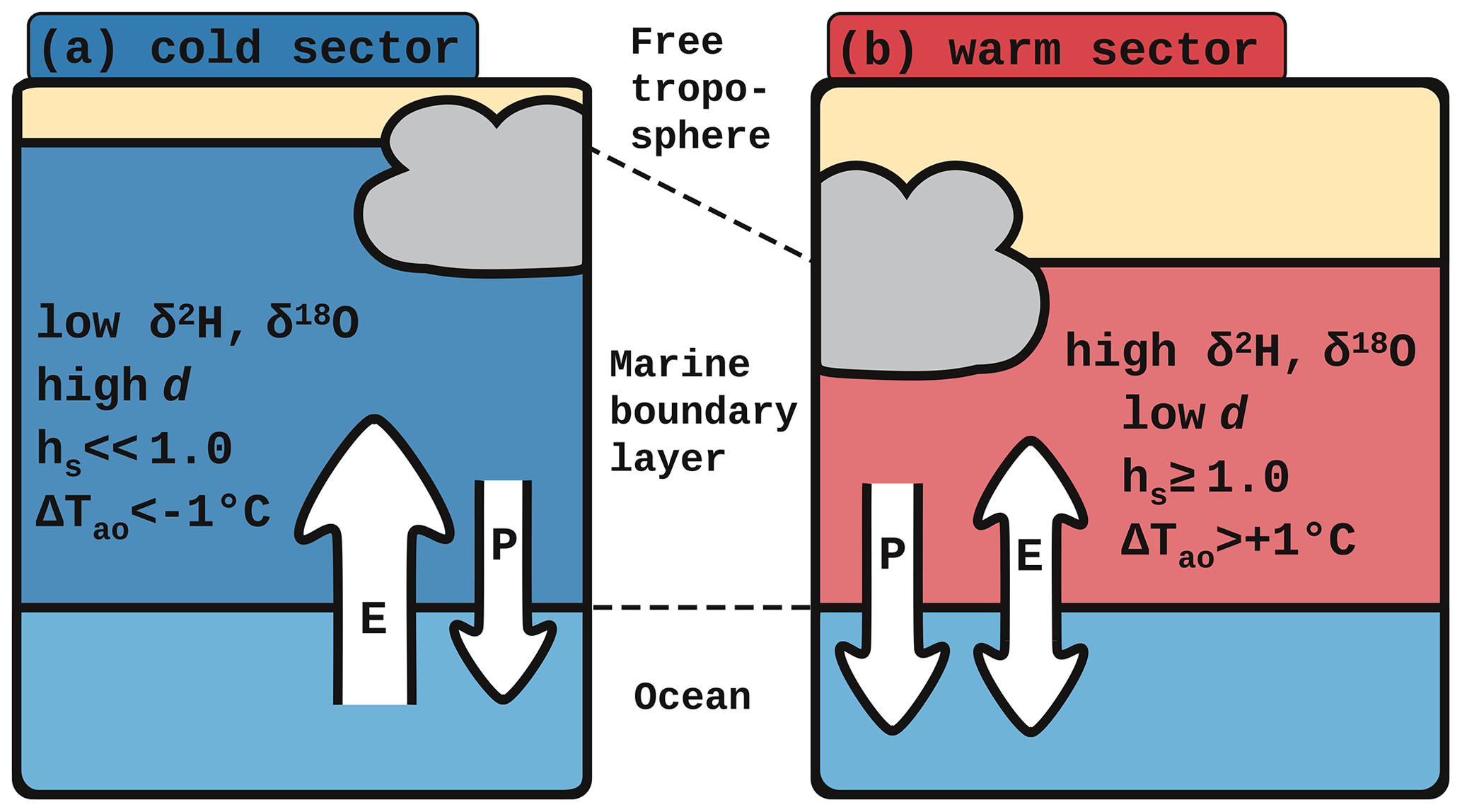
Figure 1Schematic of air–sea interactions in (a) the cold and (b) the warm sector of an extratropical cyclone. E denotes ocean evaporation and, if directed downward, dew formation, and P denotes precipitation. hs is the relative humidity with respect to sea surface temperature and ΔTao the difference between the air and sea surface temperature. For details see text.
Despite their important role in the atmospheric moisture budget, only few and regionally limited measurements of ocean evaporation and dew deposition are available, because of the extensive set of measurements needed (Pollard et al., 1983; Fleagle and Nuss, 1985; Holt and Raman, 1990; Neiman et al., 1990; Persson et al., 2005; Bharti et al., 2019). Many studies on air–sea moisture fluxes in extratropical cyclones rely on model simulations (e.g. Nuss, 1989; Beare, 2007; Sinclair et al., 2010; Boutle et al., 2011). Further insight into the strength of ocean evaporation can be gained by ship-based measurements of humidity and of stable water isotopes (SWIs) in water vapour, which provide near-surface water vapour characteristics. SWI measurements can be used to better understand the importance of various moist processes including ocean evaporation, dew deposition and precipitation for the MBL moisture budget. The relative abundance of heavy and light isotopes in the different water reservoirs is altered during phase change processes due to isotopic fractionation. The abundance of the heavy isotopologues 2H1H16O and 1HO is expressed by the δ notation (δ2H and δ18O, respectively) (Dansgaard, 1964), which is defined as the isotopic ratio R of the concentration of the heavy isotopologue to the concentration of the light isotopologue (hereafter named isotope) 1HO relative to an internationally accepted standard isotopic ratio (the Vienna standard mean ocean water, VMSMOW2; with and ): and . There are two types of isotopic fractionation: equilibrium fractionation, which is caused by the difference in saturation vapour pressure of different isotopes, and non-equilibrium fractionation, which occurs due to molecular diffusion, e.g. during ocean evaporation. A measure of non-equilibrium fractionation and, thus, diffusive processes such as evaporation or dew deposition is the second-order isotope variable deuterium excess d, defined as . During a diffusive process, a positive anomaly in d develops in the phase towards which the flux is directed (e.g. the atmosphere during ocean evaporation), while a negative d anomaly can be observed in the other, reservoir, phase (e.g. rain droplets during below-cloud evaporation). If the moisture reservoir is large and well mixed, which can be assumed for the ocean during ocean evaporation, the impact of isotopic fractionation on the isotopic composition of the reservoir can be neglected. Air–sea net moisture fluxes occur due to non-equilibrium conditions at the atmosphere–ocean interface, and, therefore, d can be used as a tracer of air–sea interactions.
Previous studies have shown that d in MBL water vapour negatively correlates with hs (Uemura et al., 2008; Pfahl and Wernli, 2008; Bonne et al., 2019; Thurnherr et al., 2020a), which reflects the differing strength of ocean evaporation and, thus, non-equilibrium fractionation in different hs environments. So far, studies focused on environments with low hs, where positive d in atmospheric water vapour has been observed due to strong ocean evaporation (Gat et al., 2003; Uemura et al., 2008; Gat, 2008; Pfahl and Wernli, 2008; Aemisegger and Sjolte, 2018). In extratropical cyclones, such low-hs environments with high d are expected in the cold sector, corresponding to areas of strong large-scale ocean evaporation (Aemisegger and Sjolte, 2018, and Fig. 1a). An opposite signal in d, i.e. d close to or below 0, is expected in the warm sector, where dew deposition or weak ocean evaporation occurs (Fig. 1b). Only few measurements of negative d in MBL water vapour have been reported (Uemura et al., 2008; Bonne et al., 2019; Thurnherr et al., 2020a), which have been related to weak ocean evaporation (Uemura et al., 2008) and deposition of water vapour on sea ice (Bonne et al., 2019). However, to our current knowledge there is no study that investigated the processes leading to the d–hs relationship in MBL water vapour in high-hs environments.
Modelling of SWIs in the atmospheric branch of the water cycle helps to identify which moist processes influence the isotopic composition of water vapour. The incorporation of SWIs into numerical climate and weather models (Joussaume et al., 1984; Yoshimura et al., 2008; Blossey et al., 2010; Risi et al., 2010b; Werner et al., 2011; Pfahl et al., 2012) allows us to study the impact of different moist atmospheric processes on the SWI evolution of atmospheric water vapour. Such model simulations also provide a spatial context to measurement data and the basis for the definition of various useful Eulerian and Lagrangian diagnostics. Recently, in situ SWI observations have been used to compare the representation of the hydrological cycle in general circulation models equipped with water isotopes, showing large differences in the performance of the three atmospheric general circulation models ECHAM5-wiso, LMDZiso and IsoGSM (Steen-Larsen et al., 2017). Detailed insights into the interaction of weather systems and SWIs can be obtained from the isotope-enabled Consortium for Small-scale Modelling model COSMOiso (Pfahl et al., 2012). Lagrangian studies based on COSMOiso simulations have shown that δ2H and d in near-surface water vapour are strongly influenced by ocean evaporation and, over land, by evapotranspiration and mixing with moist air, while liquid- and mixed-phase cloud formation contributes to the δ2H and d variability (Aemisegger et al., 2015; Dütsch et al., 2018). The importance of different air mass origins and pathways of airstreams for the SWI evolution during frontal passages has been illustrated using a COSMOiso simulation in the Mediterranean Sea (Lee et al., 2019). Idealised COSMOiso simulations of an extratropical cyclone showed that the meridional advection of air in the cold and warm sector strongly shapes the characteristic high δ values in the warm and low δ values in the cold sector (Dütsch et al., 2016, see also Fig. 1). In their idealised model study, isotopic fractionation during ocean evaporation was switched off, such that air–sea interaction processes did not affect their simulated δ2H contrast between the cold and warm sector. It is, therefore, not known yet how important air–sea interactions are in shaping the high δ values in the warm sector and the low δ values in the cold sector of extratropical cyclones (see also Fig. 1).
In this study, we aim to address the following two questions analysing 3-month ship-based SWI measurements in the Southern Ocean in combination with high-resolution regional COSMOiso simulations covering the measurement period with the goal to better understand the influence of air–sea interactions on the isotopic composition of water vapour in the MBL.
-
What are the characteristic SWI signals in the cold and warm sector of extratropical cyclones, respectively?
-
How do the differing air–sea freshwater fluxes in the cold and warm sector of extratropical cyclones affect the isotopic variability of the MBL water vapour?
This paper is structured in the following way: in Sect. 2, the measurements, simulations and Lagrangian diagnostics are described. An objective identification of cold and warm temperature advection is introduced in Sect. 3. Thereafter, the temperature advection regimes during the Antarctic Circumnavigation Expedition (ACE) are discussed (Sect. 4.1), the measured SWI signals are related to the cold and warm temperature advection in the cold and warm sector of extratropical cyclones, respectively (Sect. 4.2), and the evolution of the isotope signals along COSMOiso trajectories is analysed for trajectories from the cold and warm sector, respectively (Sect. 4.3).
This study combines meteorological and SWI measurements from ACE, which took place from 21 December 2016 to 19 March 2017 in the Southern Ocean (Walton and Thomas, 2018; Schmale et al., 2019, Sect. 2.1), with COSMOiso simulations and ERA-Interim reanalysis data from the European Centre for Medium-Range Weather Forecasts (ECMWF) (Sect. 2.2). The Lagrangian methods used for the analysis are described in Sect. 2.3.
2.1 Measurement data
Different measurement data sets from ACE were used in this study:
-
During ACE (see cruise track in Fig. 2), continuous measurements of SWIs using a Picarro cavity ring-down laser spectrometer were conducted at a height of 13.5 m a.s.l. above the ocean surface on board the Russian research vessel Akademik Tryoshnikov. A detailed description of the SWI data set (setup and post-processing) can be found in Thurnherr et al. (2020a).
-
A merged SST product (Haumann et al., 2020) was used, which is a combination of in situ measurements using an Aqualine Ferrybox system and, where no in situ measurements are available, of the daily optimum interpolation SST satellite product from the Advanced Very High Resolution Radiometer (AVHRR) infrared sensor (version 2; AVHRR-Only; Reynolds et al., 2007).
-
Air temperature, air pressure and relative humidity are used from the automated weather station operated on board (Landwehr et al., 2019).
-
Rainfall and snowfall rates along the ship track are derived from continuous micro rain radar (MRR) measurements. The rainfall rate (Gehring et al., 2020) is computed from the drop size distribution estimated from the MRR Doppler spectra at the 100–200 m a.s.l. range gate as explained in Peters et al. (2005). During time periods with a melting layer close to the surface, the rainfall rate is strongly overestimated by our method. These periods of a low melting layer (<200 m a.s.l.) are masked for the analysis in this study. The snowfall rates are calculated from the MRR effective reflectivity at the 400 m a.s.l. range. The effective reflectivity along with the Doppler velocity and the spectral range is derived from the raw Doppler spectra using the algorithm of Maahn and Kollias (2012). In order to estimate the snowfall rate, we use the reflectivity–snowfall-rate (Z–S) relationship derived by Grazioli et al. (2017) based on the measurements at Dumont d'Urville station. We assume that the snowfall measurements at this location (on an island near Adélie Land) provide a good approximation of the snowfall microphysical properties observed during ACE.
-
To study the vertical structure of the MBL, radiosonde measurement are used (Gorodetskaya et al., 2021). iMET radiosondes were deployed during ACE measuring pressure, air temperature, relative humidity and the GPS location. The radiosondes were launched once or twice per day and at higher frequency for specific events.
All data are used at an hourly time resolution, except for the radiosondes, which were launched at specific times with vertical profile measurements available at 1 s resolution.
2.2 Reanalysis and model data
2.2.1 ERA-Interim reanalysis data
Six-hourly data from the ERA-Interim reanalyses (Dee et al., 2011) from December 2016 to March 2017 are used for the analysis of cold and warm temperature advection (see Sect. 3) during ACE over the entire Southern Ocean. The data are interpolated to a 1∘ horizontal grid and 60 vertical levels. Due to fewer observational data in the Southern Hemisphere compared to the Northern Hemisphere, the model fields are expected to have a higher uncertainty in the Southern Hemisphere. Nonetheless, the 4D-Var data assimilation system used by ECMWF to compile the ERA-Interim reanalysis shows good performance in the Southern Hemisphere (Dee et al., 2011; Nicolas and Bromwich, 2011), and the uncertainties due to assimilation errors have been shown to be minor (Nicolas and Bromwich, 2011).
Based on the ERA-Interim reanalyses, cyclone frequencies were calculated using a 2D cyclone detection algorithm based on sea level pressure fields (Wernli and Schwierz, 2006; Sprenger et al., 2017). For the identification of the cyclones, pressure minima are removed where the topography exceeds 1500 m. Furthermore, surface fronts were detected following Schemm et al. (2015) using the following criteria: (i) the horizontal equivalent potential temperature gradient at 850 hPa has to be at least 3.8 K (100 km)−1, and (ii) the fronts need to have a minimum length of 500 km.
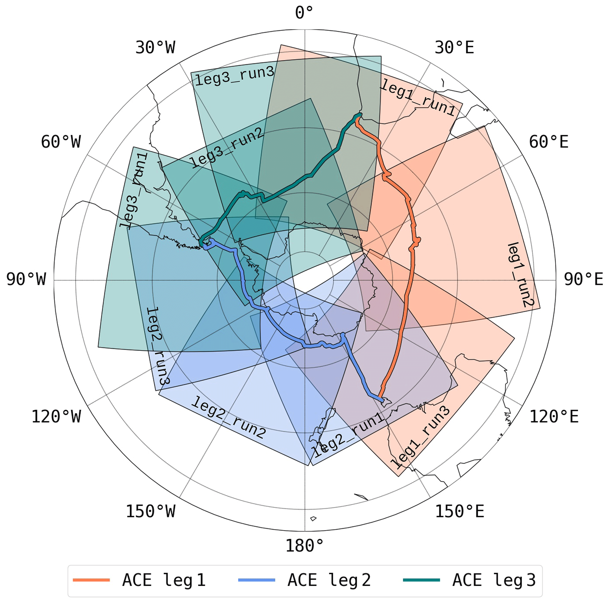
Figure 2Domains of the nine COSMOiso simulations (see also Table 1). The ACE ship track is indicated by a bold line, coloured differently for the three legs of the expedition.
2.2.2 COSMOiso simulations
The limited-area regional numerical weather prediction model COSMO (Steppeler et al., 2003) is used in its isotope-enabled version COSMOiso (Pfahl et al., 2012) with two additional parallel water cycles for the heavy water molecules HO and 1H2H16O, which mirror the water cycling of HO. These additional water cycles are affected by the same physical processes as the light water molecule, except for isotopic fractionation during phase change processes. COSMOiso has been previously used to study various aspects of the regional atmospheric water cycle over Europe and the USA (Pfahl et al., 2012; Aemisegger et al., 2015; Dütsch et al., 2018; Christner et al., 2018; Lee et al., 2019). Here, nine COSMOiso simulations were conducted over the Southern Ocean covering the ACE measurement time period. Since COSMOiso is an isotope-enabled regional numerical weather prediction model, global SWI data are needed for its initialisation and for the boundary conditions. The simulations were initialised and driven at the lateral boundaries by output from an ECHAM5-wiso simulation, which was nudged 6-hourly to temperature, surface pressure, divergence and vorticity of ERA-Interim reanalysis data (Werner et al., 2011; Butzin et al., 2014). The wind in the COSMO domain was spectrally nudged to the ECHAM5-wiso above 850 hPa to keep the meteorology within the COSMOiso domain as close as possible to the reanalysis. The ECHAM5-wiso fields are available 6-hourly with a spectral resolution of T106 (corresponding to 125 km grid spacing in meridional direction) and 31 vertical levels. The COSMOiso simulations were performed at a horizontal resolution of 0.125∘, corresponding to ∼14 km, with 40 vertical levels and explicit convection. The explicit convection setup is preferred over using the deep convection parameterisation even at a resolution of 0.125∘. Simulations with the COSMO model over Europe have been shown to represent the hydroclimate more realistically in this setup (Vergara-Temprado et al., 2019). Furthermore, isotope-enabled simulations over the Southern Ocean with explicit convection revealed a reduced strength of vertical mixing and more realistic vertical isotope profiles than simulations with parameterised convection (not shown; see also results from Jansing, 2019, with parametrised convection). Hourly outputs of the COSMOiso simulations are used for the analysis. The model domains have an area of approximately 50∘ × 50∘ and were shifted along the ACE track, such that the entire expedition route was covered by the nine simulations in space and time (see Fig. 2). Isotopic fractionation during surface evaporation is parameterised with the Craig–Gordon model (Craig and Gordon, 1965) using a wind-speed-independent formulation of the non-equilibrium fractionation factor (Pfahl and Wernli, 2009). The isotopic composition of the ocean surface water is prescribed at a constant value of 1 ‰ for δ2H and δ18O, which is relatively high for the southern part of the ACE cruise track (Xu et al., 2012), but we expect that this has minor effects for the purposes of this study. For a detailed description of the physics and isotope parameterisations in the COSMOiso model, see Doms et al. (2013) and Pfahl et al. (2012), respectively. For terrestrial surfaces, a one-layer surface snow model with equilibrium fractionation during snow sublimation and a multi-layer soil model (see Supplement of Christner et al., 2018) is used. The specifications of each model run are summarised in Table 1. The first week of each run is used as spin-up time and is not included in the analysis. For comparison with the ACE measurements, the lowest model level of the different variables is bilinearly interpolated along the ACE track. This corresponds approximately to the height of the inlet on the ship. During time periods, when two model runs overlap in time and space, one of the runs is chosen in such a way that the individual cold and warm temperature advection events are extracted entirely from one single model run.
Table 1Specifications of COSMOiso model simulations. The columns “Centre” and “Width” refer to the centre and width of the simulation domain. The column “Time window” shows the time period over which trajectories were calculated for the respective simulation. In column “Trajs”, the total number of trajectories arriving during cold and warm temperature advection (total) and the percentage of these trajectories included in the analysis based on the explained moisture fraction threshold (% incl.) are shown for each model simulation.

2.3 Backward trajectories and moisture sources
Air parcel trajectories are calculated 7 d backward using the Lagrangian analysis tool LAGRANTO (Wernli and Davies, 1997; Sprenger and Wernli, 2015) based on the three-dimensional 1-hourly wind fields from the COSMOiso simulations. The trajectories were launched every hour along the ACE track at pressure levels in 10 hPa steps between the surface and the MBL top as identified by COSMOiso. Trajectories were analysed until they left the model domain and for the time windows of each model run as indicated in Table 1. Several variables were interpolated along the trajectory positions, including the SWI concentrations, such that the evolution of the SWI composition during the air mass transport can be analysed.
Moisture sources of the MBL water vapour along the ACE track were calculated using the moisture source diagnostic developed by Sodemann et al. (2008) adjusted to identify the moisture sources of water vapour (Pfahl and Wernli, 2008) using the 7 d COSMOiso backward trajectories in a setup as in Aemisegger et al. (2014). In short, this method considers the mass budget of water vapour in an air parcel. Moisture uptakes are registered whenever the specific humidity along an air parcel trajectory increases. The weight of each uptake depends on its contribution to the specific humidity of the trajectory upon arrival. If precipitation occurs (i.e. a decrease in specific humidity along the trajectory happens) after one or several uptakes, the weight of all previous uptakes is reduced proportionally to their respective contribution to the loss. The moisture source conditions identified for each trajectory are subsequently weighted by the air parcel's specific humidity at the arrival in the boundary layer. This is done for different variables that are relevant for characterising the moisture source conditions, such as the time of uptake, the latitude and the water vapour's isotopic composition. More details on the moisture source identification algorithm is provided in the Supplement. For the COSMOiso analyses in Sect. 4, only trajectories for which at least 70 % of the moisture upon arrival can be explained by moisture uptakes along the trajectories are used. This corresponds to 90 % of all trajectories arriving during cold and warm temperature advection along the ACE track (see also Table 1) and explains the origin of, on average, 86 % of the moisture upon arrival.
The entrance time of the trajectories into a cold or warm sector before arrival at the measurement site is defined as the time when the trajectory enters the cold or warm sector (identified as explained in Sect. 3) without leaving the cold or warm sector, respectively, afterwards for more than 12 h before arrival. The 12 h criterion is used to avoid that the entrance time is affected by short residence times outside of the sector.
During the meridional advection of air in the cold and warm sector of extratropical cyclones, temperature advection occurs due to cold air, which is advected equatorward, and warm air, which is transported poleward. Temperature advection is defined as , where u is the velocity vector and T the air temperature. To calculate , the spatial distribution of T is needed, which is usually not available from ship-based meteorological measurements. Since the advection of air masses leads to a thermal imbalance between the ocean and the atmosphere, we use a simple identification method of temperature advection based on the air–sea temperature difference , where T is taken at a suitable near-surface level. A specific threshold of ΔTao is chosen to define cold and warm temperature advection, respectively. In this study, we analyse situations in which the atmosphere and the ocean are not in thermodynamic equilibrium. Therefore, symmetric thresholds around an isothermal near-surface stratification are chosen. Cold temperature advection is defined as time periods when ∘C and warm temperature advection when ΔTao>1.0 ∘C. A zonal or weak advection regime is defined for −1.0 ∘C ∘C. The effects of using different temperature thresholds to define the temperature advection regimes are discussed in Hartmuth (2019).
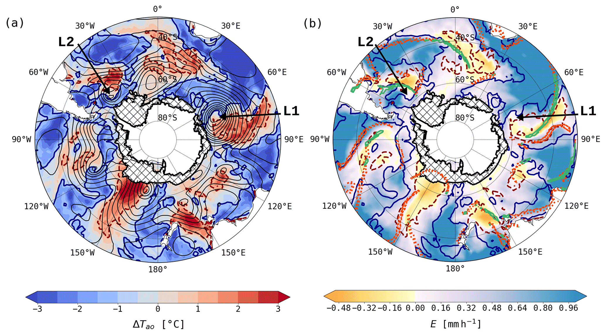
Figure 3An example of cold and warm temperature advection events in the Southern Ocean at 12:00 UTC on 26 December 2016 from ERA-Interim. (a) Air–sea temperature difference ΔTao using T at 10 m a.s.l. (colours). Grey contours show sea level pressure in 5 hPa intervals. (b) Ocean evaporation E (colours) and surface cold (green contours) and warm (orange contours) fronts. Contours of ∘C (blue, solid) indicate cold temperature advection events and of ΔTao=1.0 ∘C (red, dashed) warm temperature advection events, respectively. Land areas and areas covered by at least 1 % sea ice are blanked. Additionally, the blanked sea ice areas are hatched. L1 and L2 mark cyclones discussed in the text.
Two-dimensional masks of cold and warm temperature advection events as identified by the proposed scheme in ERA-Interim using T at 10 m a.s.l. are shown as an example at 12:00 UTC 26 December 2016 in Fig. 3. The warm temperature advection masks cover areas to the north-east of low-pressure systems (indicated by minima in sea level pressure), which correspond to the warm sectors of extratropical cyclones over the Southern Ocean (Fig. 3a). West of the low-pressure systems, cold temperature advection in the cold sectors can be seen. For example between 60 and 90∘ E, the cold and warm sectors of a large low-pressure system (L1 in Fig. 3) are indicated by the cold and warm temperature advection masks. In this snapshot, areas of cold and warm temperature advection coincide with positive and negative ocean evaporation, respectively (Fig. 3b). Cold temperature advection is associated with strong ocean evaporation. Weak ocean evaporation occurs mainly between the advection masks, and very small or even negative moisture fluxes indicate dew deposition occurring in the warm sectors (see for example cyclone L2 between 60 and 30∘ W in Fig. 3b). As expected, the surface fronts often mark the boundaries between the cold and warm sectors and, thus, of the cold and warm temperature advection masks. The warm and cold fronts of the cyclone L2 delimit the warm sector along its southern edge following closely the temperature advection mask. In other cases, the surface fronts are not aligned with the temperature advection mask. This is the case for the cyclone L1, where the cold front is within the warm temperature advection mask and negative ocean evaporation is seen behind the cold front. This discrepancy between the surface fronts and the temperature advection masks could be caused by differences in the identification schemes. The surface fronts are identified using horizontal gradients in equivalent potential temperature at 850 hPa, while the advection mask is based on the contrast between T at 10 m a.s.l. and SST. The focus on air–sea interactions in this study justifies the choice of an identification scheme based on surface fields. Ocean evaporation aligns well with the advection masks, confirming that the proposed identification scheme is useful for the investigation of air–sea fluxes. This scheme is a simple objective method and can be applied to model simulations as well as measurement data. Other Eulerian features of extratropical cyclones, such as the cyclone centres, areas or fronts, have been identified using automated identification schemes (e.g. Lambert, 1988; Hewson, 1998; Wernli and Schwierz, 2006; Jenkner et al., 2010) and used to characterise the impact of extratropical cyclones on air–sea interactions (Papritz et al., 2014; Aemisegger and Papritz, 2018). The temperature advection scheme presented here provides the possibility to study the contrasting behaviour of air–sea interactions specifically in the cold and warm sectors of extratropical cyclones, respectively.
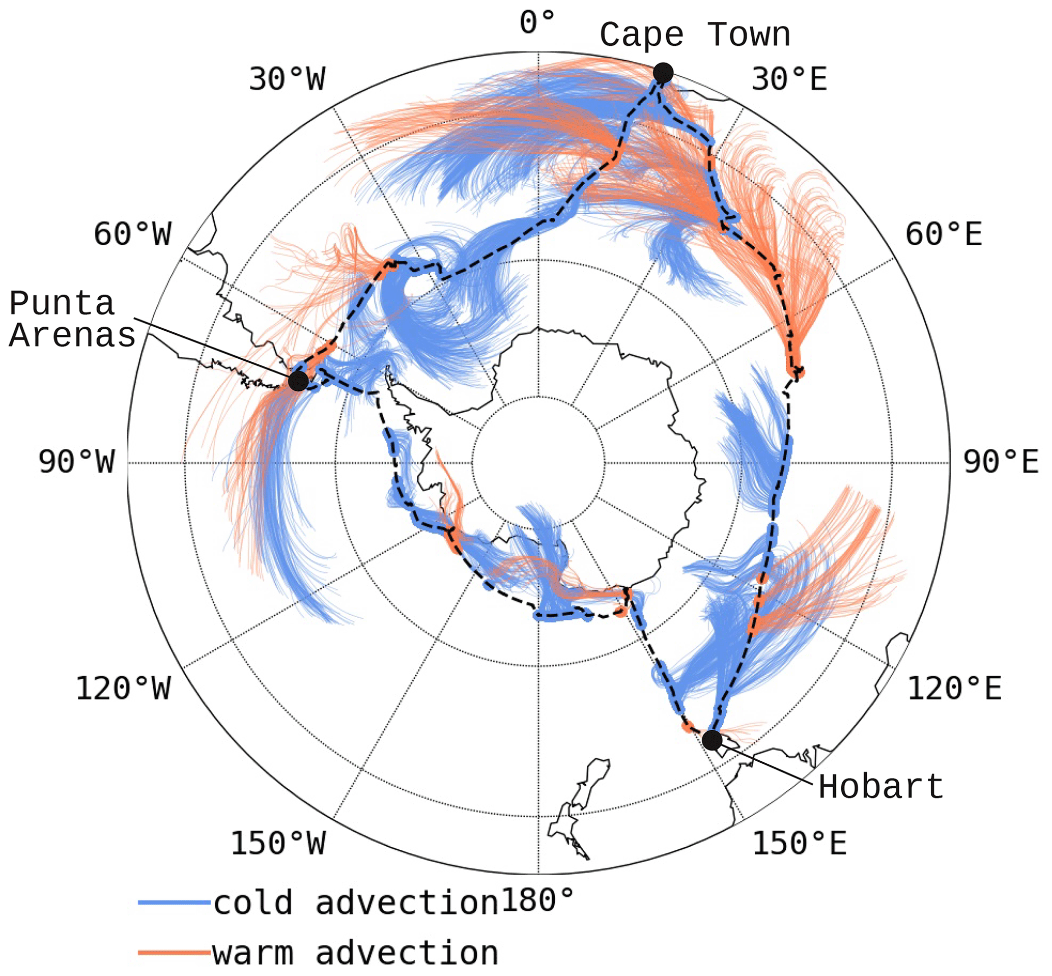
Figure 4The 2 d backward trajectories calculated with COSMOiso wind fields for warm (orange) and cold (blue) temperature advection events as identified using ΔTao in COSMOiso along the ACE ship track (black, dashed line). The black dots denote the harbour stays at Cape Town (ZA) on 21 December 2016, Hobart (AUS) from 19 to 22 January 2017, Punta Arenas (CL) from 22 to 26 February 2017 and again in Cape Town on 19 March 2017.
In this study, the cold and warm temperature advection scheme was applied (i) to the ACE measurements, which are used for the characterisation of the isotopic signal in the cold and warm sectors, using the measured air temperature at 24 m a.s.l., and the merged SST product (see Sect. 2.1); (ii) to the ERA-Interim reanalysis, which is used for a characterisation of cold and warm temperature advection during ACE, using T at 10 m a.s.l.; and (iii) to the COSMOiso data set, which is used to study the relevant processes shaping the SWI signal in cold and warm sectors, using T at the lowest model level, which corresponds to approximately 10 m a.s.l. The higher level of air temperature used for the calculation of the measured advection events leads to slightly higher frequencies in cold temperature advection and lower frequencies in warm temperature advection compared to the COSMOiso and ERA-Interim advection events, because lower air temperature is expected at higher altitude. In COSMOiso, the median temperature difference between the lowest model level at 10 m a.s.l. and the second lowest model level at 35 m a.s.l. is 0.25 [0.19, 0.29] ∘C (the brackets denote the [25, 75] percentile range). Using the temperature at 35 m a.s.l. instead of 10 m a.s.l. leads to an increase in total hours of cold temperature advection by 13 % and a decrease in warm temperature advection by 9 % along the ACE track. Nonetheless, the difference between 10 and 24 m a.s.l. air temperature is fairly small, and the advection frequencies in COSMOiso and ERA-Interim are similar to the advection frequencies in the measurements. The choice of air temperature altitude mainly changes the length of the advection events by a few hours. Overall, the identified cold and warm temperature advection events using COSMOiso agree well with the measurements and represent similar environmental conditions (see also Sect. 4.2). The COSMOiso backward trajectories along the ACE track show further that the identified cold and warm temperature advection events generally refer to situations of northward and southward flow, respectively (Fig. 4). We conclude that the proposed identification scheme is adequate to study the impact of meridional air mass advection on air–sea moisture fluxes in measurements and simulations.
4.1 Temperature advection regimes and their vertical structure during ACE
(a) Occurrence frequencies of the advection regimes over the Southern Ocean
In order to characterise the temperature advection regimes, the frequency of the advection regimes at each grid cell (referred to as occurrence frequency in the following) and the associated air–sea moisture fluxes (i.e. the mean values associated with each advection regime) are calculated in the region south of 30∘ S for the period from December 2016 to March 2017 based on ERA-Interim. The spatial patterns of cold temperature advection, warm temperature advection and zonal flow south of 30∘ S in the ACE summer (December 2016–March 2017, Fig. 5) are in general agreement with the December–March climatology over the period 1979–2018 (see Fig. S1 in the Supplement). Therefore, we will focus on the occurrence frequencies of temperature advection during ACE in the following. Cold temperature advection, warm temperature advection and zonal flow occur with different frequencies south of 30∘ S (Fig. 5). Zonal flow is the most frequently occurring advection regime (54 %), the median air–sea fluxes lie in between the values for cold and warm temperature advection, and the net air–sea moisture flux is close to zero. Therefore, we will mainly discuss cold and warm temperature advection in the following, which occur with frequencies of 32 % and 14 %, respectively. Each temperature advection regime, thus, occurs frequently and represents an important large-scale flow situation of the atmospheric dynamics over the Southern Ocean. In the following, the large-scale flow environment and freshwater fluxes associated with cold and warm temperature advection are discussed separately.
Cold temperature advection occurs during the meridional transport of cold air over a relatively warmer ocean surface in the cold sector of extratropical cyclones. A high occurrence frequency of cold temperature advection of up to 60 % is seen in a latitudinal band north of 40∘ S, equatorward of regions with high cyclone frequencies in all three ocean basins (Fig. 5a). In these areas, the cold sectors of extratropical cyclones pass over regions with anomalously warm SSTs, which are higher than the zonal mean SST (Fig. 6). For instance in the south-eastern Indian Ocean, the two zonal SST maxima at 20 and 60∘ E north of 40∘ S overlap with the local frequency maxima of cold temperature advection. In these regions, hot spots of large-scale ocean evaporation occur frequently and are associated with the warm ocean western boundary currents along the continents (Moore and Renfrew, 2002; Aemisegger and Papritz, 2018). Cold temperature advection also frequently occurs along the Antarctic coast in the Ross Sea, in the Weddell Sea and across the Amery Ice Shelf. These areas correspond to regions of frequent cold air outbreaks in summer (Papritz et al., 2015). During cold air outbreaks, which are often induced by extratropical cyclones, cold and dry air is advected over a relatively warm ocean. In the same regions along the Antarctic coast, strong large-scale ocean evaporation events occur, of which more than 80 % are driven by extratropical cyclones (Aemisegger and Papritz, 2018). Strong evaporation is therefore expected to occur during cold temperature advection. Surface evaporation during cold temperature advection is found to be positive with a mean value and standard deviation of 0.08±0.05 mm h−1 (Fig. 5b) and increases towards the Equator due to the SST dependence of ocean evaporation. Small amounts of rainfall are associated with cold temperature advection (mean value of 0.05±0.04 mm h−1) and are mainly due to shallow convection behind the cold front. The net air–sea moisture flux during cold temperature advection is from the ocean into the atmosphere (Fig. 5b).
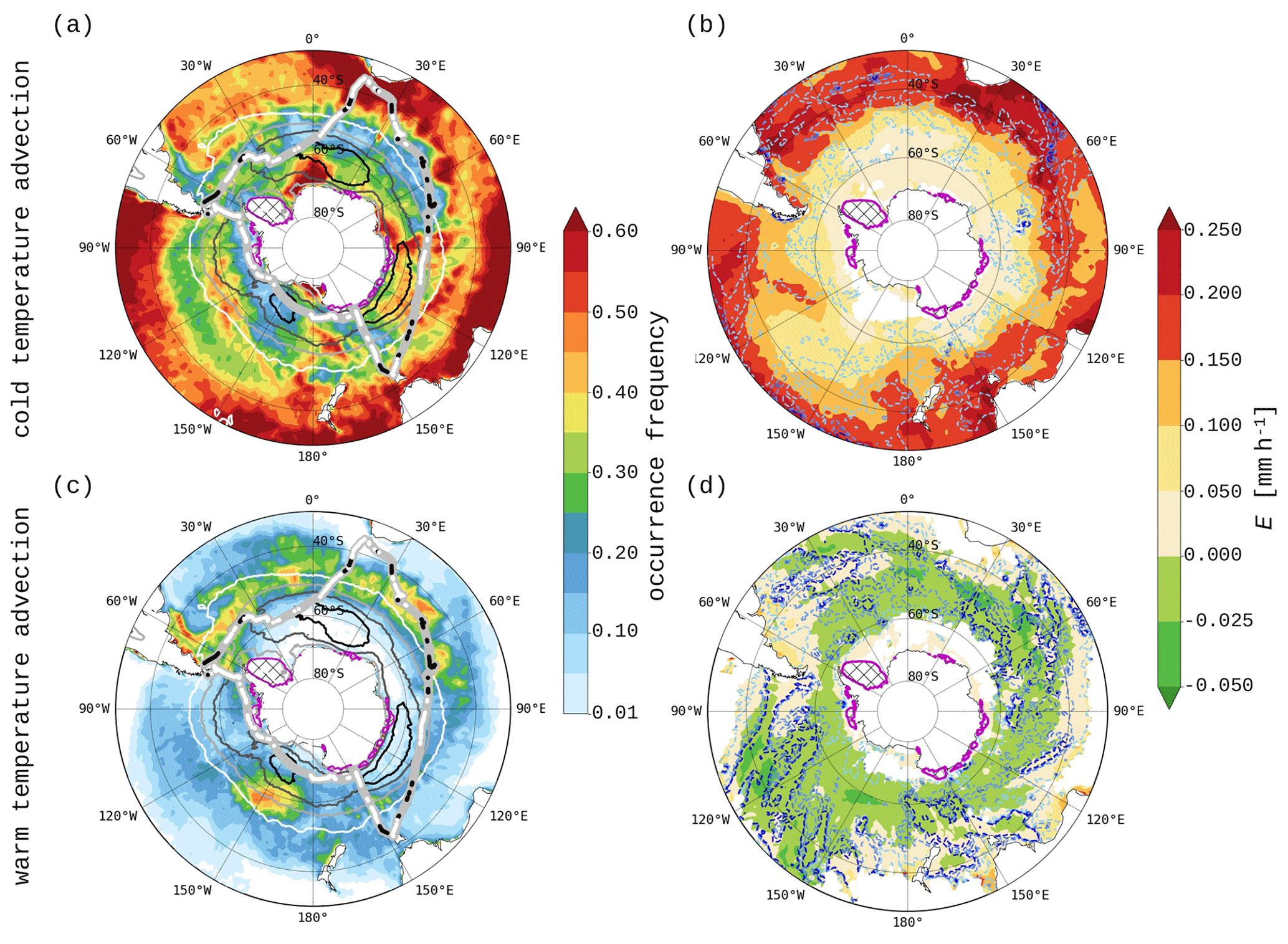
Figure 5Mean occurrence frequencies of cold and warm temperature advection (a, c) and the associated ocean evaporation (b, d) from December 2016 to March 2017 using ERA-Interim. Contours in panels (a) and (c) show the cyclone frequencies of 10 %, 20 %, 30 % and 40 % (from white to black, respectively). Blue dashed lines in panels (b) and (d) show mean surface precipitation in the respective flow category at levels of 0.06, 0.18, 0.24 and 0.3 mm h−1 (from light to dark blue, respectively). The grey thick line in panels (a) and (c) shows the ACE ship track with the observed occurrences of cold (white points) and warm (black points) temperature advection events during ACE. Land areas and areas covered by at least 50 % sea ice are blanked. Additionally, the blanked sea ice areas are hatched and bounded by pink contours.
Warm temperature advection frequently occurs in a few areas in the Southern Ocean where warm air is transported over a relatively colder ocean. Warm temperature advection hot spots of up to 50 % occurrence frequency can be observed north of the region with highest cyclone frequency and south of the band of high cold temperature advection occurrence frequency (Fig. 5c). These regions are associated with the warm sectors of extratropical cyclones along the Southern Ocean storm track, in which warm and moist air is advected polewards. Furthermore, warm temperature advection occurs along the eastern coast of South America and at 150∘ W in the South Pacific, which are regions of anomalously cold ocean waters (Fig. 6). The isolated hot spot in the Pacific is connected to the location of the oceanic polar front, which has its northernmost position between 55 and 60∘ S in the Pacific Ocean around 150∘ W (Moore et al., 1999). The advection of terrestrial and/or subtropical air over the cold Malvinas current along the Argentinian coast leads to frequent warm temperature advection along the east coast of South America. During warm temperature advection, surface evaporation is low or negative, with a mean of 0.00±0.02 mm h−1 (Fig. 5d). Furthermore, warm temperature advection is accompanied by precipitation with a mean of 0.16±0.14 mm h−1. Thus, there is a net flux of moisture from the atmosphere into the ocean during warm temperature advection.
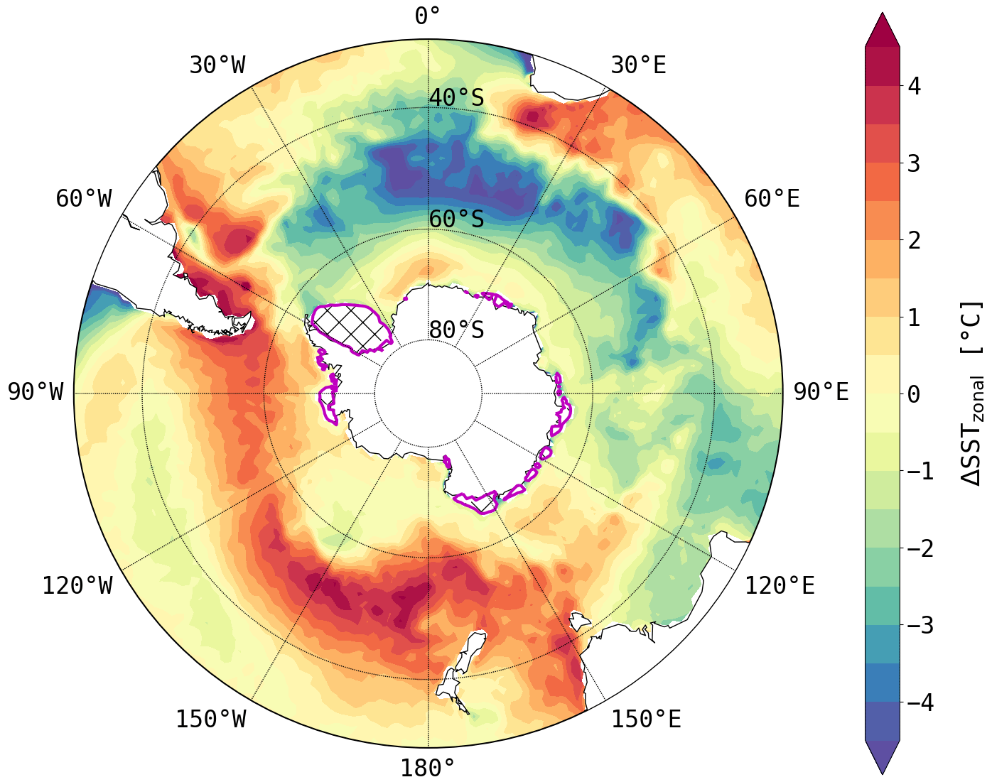
Figure 6Deviations of the sea surface temperature from the zonal mean from December 2016 to March 2017 using ERA-Interim. Land areas and areas covered by at least 50 % sea ice are blanked. Additionally, the blanked sea ice areas are hatched and bounded by pink contours.
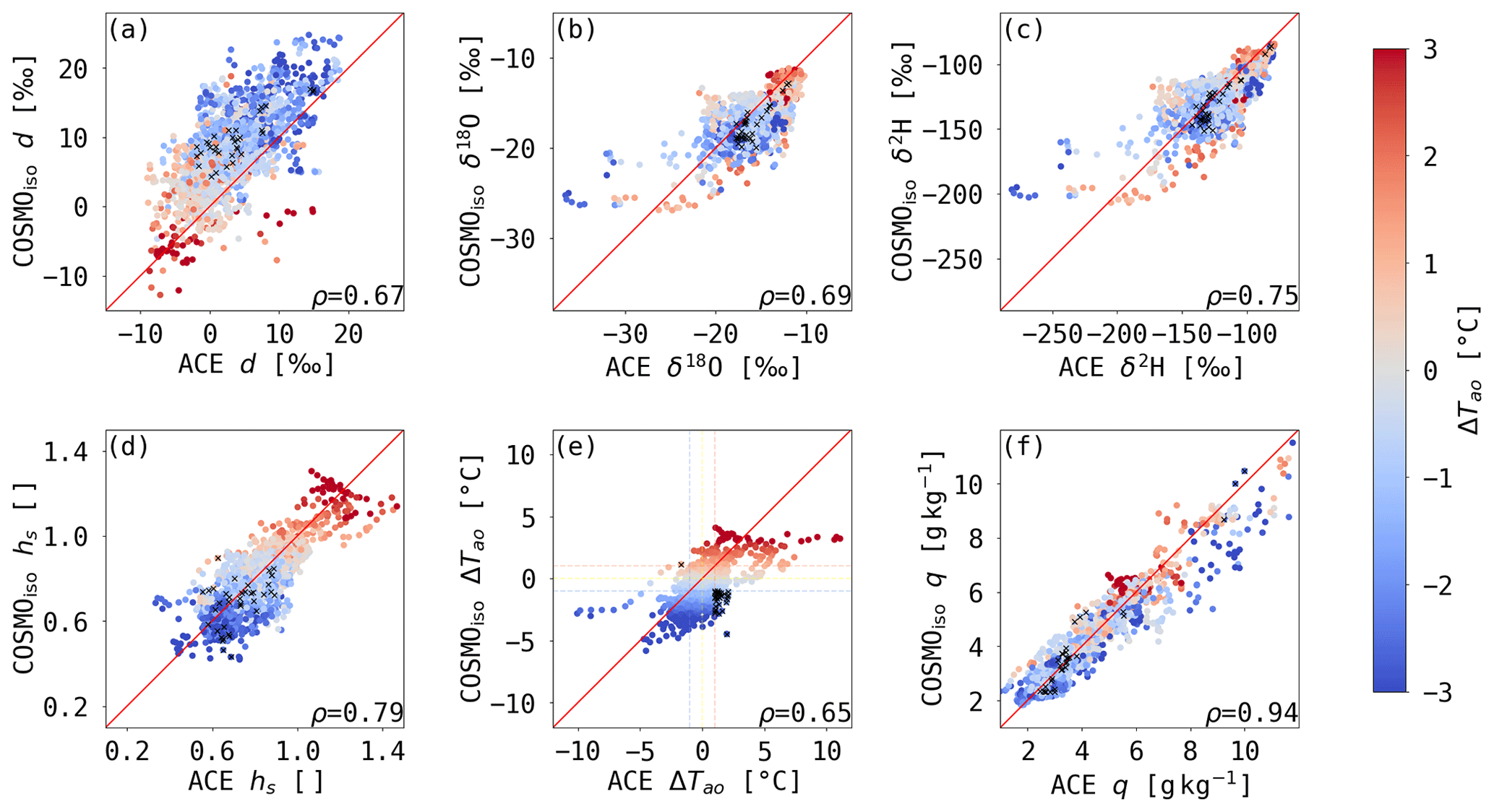
Figure 7Scatterplots of 1-hourly ACE measurements vs. interpolated values from COSMOiso simulations at the lowest model level along the ACE ship track of (a) d, (b) δ18O, (c) δ2H, (d) hs, (e) air–sea temperature difference ΔTao and (f) specific humidity q coloured by ΔTao from COSMOiso. Points with contradicting cold and warm temperature advection classification between the measurements and simulations are marked with black crosses. The value of the Pearson correlation coefficient ρ for each variable is shown in the bottom right of the panels.
(b) Advection regimes along the ACE track
Specifically along the ACE track, the occurrence frequencies of the three advection regimes differ from the occurrence frequencies over the entire Southern Ocean. In the ACE measurements, 59 % of all advection events were zonal, 27 % cold and 14 % warm temperature advection events (see black and white dots in Fig. 5a, b). The frequency of cold temperature advection events along the ACE track is approximately 6 % lower than in the climatology for the region south of 30∘ S (Fig. 5a). The ACE track was close to Antarctica only in the Pacific, which means that cold air outbreaks in the Atlantic and Indian Ocean, where the ACE track was mostly located in areas with zonal and warm temperature advection, are undersampled (see also Fig. 5). Warm temperature advection events were mainly encountered in the South Indian and Atlantic Ocean. Therefore, insight from the ACE data set on warm temperature advection is representative for these two ocean basins around Antarctica.
The largest difference in the identification of cold and warm temperature advection between the measurements and COSMOiso is observed during leg 2 (compare orange trajectories in Fig. 4 and black dots in Fig. 5). Two warm temperature advection events are identified during leg 2 in COSMOiso, which were categorised as zonal flow using the measurements. During these two events, air is advected northwards from Antarctica towards the ship's position. The large positive ΔTao in COSMOiso could be caused by adiabatic warming during the descent in a katabatic wind event. These two warm temperature advection events thus differ from a typical warm temperature advection event as generally observed along the ACE track in the warm sector of an extratropical cyclone.
Although zonal flow events dominated, a total measurement time of 462 h during cold and 238 h during warm temperature advection, respectively, is available, which provides an observational data set that is large enough to statistically analyse the typical isotope signature associated with these events.
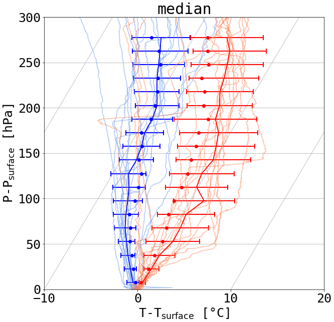
Figure 8Skew T–P diagram of air temperature relative to the surface air temperature from radiosoundings (thin lines) during cold (blue) and warm (red) temperature advection events. The y axis shows the pressure relative to the surface pressure. The thick lines and error bars show the median and standard deviation in every 15 hPa pressure bin. The dots show the median profiles from COSMOiso for the same cold and warm temperature advection events as sampled by the radiosoundings.
(c) Vertical temperature profiles and precipitation
The strongly differing environmental conditions during cold and warm temperature advection, as seen in the ERA-Interim composite analysis (Fig. 5), can also be observed in the ACE measurements. A distinctively different hs during cold compared to warm temperature advection was observed (see e.g. Fig. 7d) with a median value of 70.9 % during cold and 96.9 % during warm temperature advection, respectively. This is in agreement with the results from the ERA-Interim composites, which show the strongest positive air–sea moisture fluxes in the cold temperature advection regime and low or negative fluxes in the warm temperature advection regime.
The vertical temperature profiles also differ strongly between cold and warm temperature advection. Radiosoundings during cold temperature advection show a conditionally unstable MBL up to 130 hPa a.s.l. (Fig. 8). With a median surface pressure of 988 hPa, this corresponds to a median MBL top at 848 hPa. During warm temperature advection, the median profile from radiosoundings shows a stable MBL starting from the surface. The individual soundings during warm temperature advection are very diverse. Most of them show a strong temperature inversion below 50 hPa a.s.l., which corresponds to a MBL top at 930–960 hPa, indicating a shallow MBL. The entire MBL is, thus, influenced by the opposite air–sea heat fluxes and resulting mixing processes during cold and warm temperature advection.
As indicated by the ERA-Interim climatology (Fig. 5b, d), precipitation characteristics differ between cold and warm temperature advection. The precipitation rates along the ACE track (derived from MRR measurements) show that during cold temperature advection rainfall (>0 mm h−1) occurred during 25 % and snowfall during 14 % of the time. The median value of the rainfall rate was 0.16 mm h−1 and for the snowfall rate 0.04 mm h−1. During warm temperature advection, rainfall was present 32 % of the time and no snowfall occurred, leading to a smaller total precipitation occurrence frequency than during cold temperature advection. However, precipitation during warm temperature advection was more intense, with a median value of 0.31 mm h−1. Surface precipitation in ERA-Interim (Fig. 5b, d) and COSMOiso (not shown) shows larger median values for cold and warm advection but qualitatively agrees with the observed rainfall intensities with typically heavier precipitation during warm than cold temperature advection. The reasons for the mismatch between the observed and modelled precipitation amounts include (i) limitations of the microphysical scheme used in numerical weather models, specifically for mixed-phase clouds; (ii) uncertainties in the micro-rain-radar-derived precipitation amounts; and (iii) discrepancies between point measurements (as provided by the radar) and the model's grid averages. Nevertheless, overall we assume that the simulated precipitation statistics are fairly realistic. Even though precipitation during cold temperature advection is less intense, it occurs more often, resulting in a larger input of precipitation into the ocean. The larger precipitation totals during cold compared to warm temperature advection events are mainly due to the difference in the average geographical extent of the two advection regimes. Cold temperature advection generally occurs over much larger areas than warm temperature advection, which is usually confined to the warm sectors of extratropical cyclones, which leads to shorter sections of warm temperature advection along the ship track, respectively (black dots in Fig. 5b).
Overall, the observed environmental conditions during ACE are in agreement with the climatological composite analysis of cold and warm temperature advection based on ERA-Interim. In the next sections, we will discuss the isotopic signature during cold temperature advection, warm temperature advection, and zonal flow (Sect. 4.2) and the processes shaping the differing isotopic signature of MBL water vapour during cold and warm temperature advection (Sect. 4.3).
4.2 Observed and simulated SWI composition during the different advection regimes
(a) ACE observations
To identify the characteristic SWI signal during cold and warm temperature advection, the measured isotope and environmental variables during ACE are analysed with respect to the different temperature advection regimes. The distributions of δ2H, δ18O and d during warm temperature advection, cold temperature advection and zonal flow are shown in Fig. 9. For all isotope variables, the distributions associated with the cold and the warm temperature advection regime are significantly different when applying a Wilcoxon rank-sum test (p<0.01). The mode of the d distribution during cold temperature advection is 6.3 ‰ higher than during warm temperature advection. The median d during cold temperature advection is 6.1 ‰ compared to −0.3 ‰ during warm temperature advection. The distributions of δ2H and δ18O are similar, with median values 27.9 ‰ and 3.8 ‰ higher during warm compared to cold temperature advection, respectively. The mode of the distributions is higher by 34.0 ‰ for δ2H and 4.2 ‰ for δ18O during warm compared to during cold temperature advection. The median and mode of the zonal flow lie in between the respective values of the cold and warm temperature advection distributions for all isotope variables.
As already shown in previous studies (Uemura et al., 2008; Pfahl and Wernli, 2008; Steen-Larsen et al., 2014b; Benetti et al., 2015; Bonne et al., 2019; Thurnherr et al., 2020a), d in the MBL is anti-correlated with the near-surface relative humidity. In the ACE measurements, d and hs negatively correlate, with a Pearson correlation of −0.73. During cold temperature advection, the atmosphere is undersaturated (low hs), and during warm temperature advection it is close to saturation or oversaturated (hs≥100 %, Fig. 7d). Therefore, contrasting atmosphere–ocean moisture fluxes, which can even be of opposite sign, can be associated with cold and warm temperature advection. The ACE measurements confirm the expected contrasts in the isotopic signature and the close link of d and hs also in oversaturated conditions.
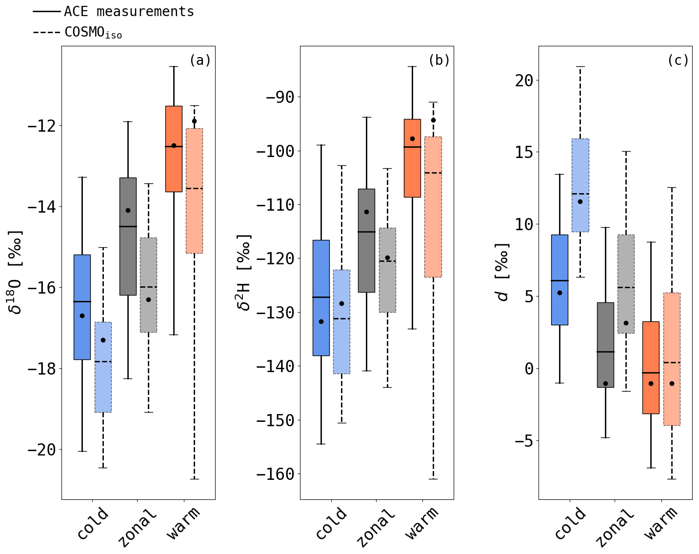
Figure 9Box plots showing median (black horizontal line in box), interquartile range (boxes), mode (black dots) and [5, 95] percentile range (whiskers) of (a) δ18O, (b) δ2H and (c) d from ACE measurements (solid lines, dark colours) and COSMOiso simulations at the lowest model level (dashed lines, light colours) during cold temperature advection (blue), zonal flow (grey) and warm temperature advection (orange).
(b) COSMOiso simulations
From the air–sea fluxes associated with the different temperature advection regimes, we expect the MBL to be strongly influenced by ocean evaporation during cold temperature advection, whereas dew deposition on the ocean surface plays a major role in shaping the observed isotopic composition of water vapour during warm temperature advection. To better understand how the observed anomalies in the isotope signals form during cold and warm temperature advection, the isotopic composition and other environmental variables are analysed along the ACE track using COSMOiso simulations. For 1 % of all 1-hourly measurement points of the ACE legs 1–3, the classification of cold and warm temperature advection according to the COSMOiso simulations disagrees with the observed classification (see black crosses in Fig. 7). These measurement points and their associated trajectories are excluded from the following analysis. The very low ∘C and very high ΔTao>7.0 ∘C in the ACE measurements are not seen in COSMOiso (Fig. 7e). These instances belong to a katabatic wind event and a vertical dry intrusion event, respectively, for which COSMOiso did not correctly simulate the meteorology. These events are included in the analysis as the identification of cold or warm temperature advection agrees in the model and the measurements.
The simulated isotope variability is in agreement with the measurements with a Pearson correlation coefficient ρ of 0.75 for δ2H, 0.69 for δ18O and 0.67 for d (Fig. 7). COSMOiso reasonably reproduces the measured SWI variability and composition during ACE. The same qualitative distribution of the cold and warm temperature advection SWI signal is seen with a shift in δ2H and δ18O towards negative values for all temperature advection regimes and a shift in d towards positive values during cold temperature advection and zonal flow compared to the measured composition during ACE (Fig. 9). This difference specifically during conditions with important contributions of water vapour to the MBL by ocean evaporation could be caused by too strong a vertical mixing in the COSMOiso simulations. This effect could also lead to the slightly lower specific and relative humidity in the simulation compared to the measurements (Fig. 7d, f). The vertical temperature gradient in the MBL can be used as a measure of vertical mixing. During cold advection, the vertical temperature structure in the MBL is generally simulated well by COSMOiso (Fig. 8). The simulated median vertical temperature profile shows a temperature inversion around 150 hPa a.s.l., which lies above the inversion in the measured profiles at 130 hPa a.s.l. This supports the hypothesis that COSMOiso has too strong a vertical mixing as a higher inversion height implies more mixing. Furthermore, too strong an entrainment at the MBL top in COSMOiso could also contribute to the observed difference in SWIs during cold temperature advection. These findings show that the environmental conditions during cold temperature advection, i.e. during conditions of strong ocean evaporation, are not well reproduced in COSMOiso. The simulated median temperature profile during warm advection shows, in accordance with the measured profile, a stable MBL. Due to the model's vertical resolution, very strong temperature inversions in the radiosoundings are not represented in the simulated profiles. This is most likely the reason for the negative temperature bias in the simulated profiles during warm advection.
A further reason for the differences between the measurements and simulations could originate from the formulation of non-equilibrium isotopic fractionation in COSMOiso. Using a weaker, wind-independent formulation of the non-equilibrium fractionation factor by Merlivat and Jouzel (1979) (in the smooth regime at 6 m s−1) instead of the currently used formulation by Pfahl and Wernli (2009) in COSMOiso simulations with parameterised convection leads to a decrease in d by, on average, 2 ‰, on the lowest model level over the ocean surface (Jansing, 2019). The larger negative bias in δ18O compared to δ2H in COSMOiso could also be explained by too strong a non-equilibrium fractionation using the formulation by Pfahl and Wernli (2009). However, the simulations using the formulation by Merlivat and Jouzel (1979) also show a decrease in d variability above oceanic areas (Jansing, 2019). As we are interested in the processes shaping the SWI variability in the MBL, the formulation by Pfahl and Wernli (2009) is more adequate to use here as the SWI variability in the measurements and simulations agrees well.
To better understand the difference in SWIs between measurements and COSMOiso simulations, further studies are needed such as the detailed analysis of case studies based on extensive 3D data sets as, for example, collected during the Iceland Greenland Seas Project (Renfrew et al., 2019). Even though near-surface simulated and measured isotope signals do not agree everywhere, the COSMOiso simulations capture the observed variability of the isotopic composition and provide similar distributions of isotope variables as the observations for the three advection categories. These simulations will thus be used for an assessment of the relevant processes shaping the isotopic composition of water vapour in the MBL during cold and warm temperature advection.
4.3 Formation of isotope anomalies during cold and warm temperature advection
During transport, the specific humidity of air masses varies due to different moist atmospheric processes such as ocean evaporation, dew deposition, cloud formation and below-cloud evaporation. These processes might alter the isotopic composition of the water vapour substantially between the moisture source and the point of measurement. With a Lagrangian composite analysis of cold and warm temperature advection events, we aim to assess the relative importance of these processes in shaping the SWI composition of water vapour in the MBL. One way to analyse how such moist processes during transport affect the SWI composition of the air mass is to compare the air mass' properties at the moisture source and upon arrival at the measurement site (Fig. 10). The weighted mean of the moisture source properties of the MBL water vapour along the ACE track is computed using 7 d backward trajectories from 3D COSMOiso wind fields and is compared to the properties of the trajectories at the arrival and at the driest point in terms of specific humidity along the backward trajectories.
(a) Cold temperature advection
For cold temperature advection, the weighted mean moisture uptake time is 37 [26, 48] h (the numbers in the brackets denote the [25 %, 75 %] percentile range) before the air parcels arrived at the measurement site (Fig. 10e). The air parcels enter the cold sector 49 [31, 91] h before arrival, and, thus, the bulk of the moisture of the cold air is taken up in or shortly before entering the cold sector. After the uptake, small changes in δ2H, δ18O and d between the moisture source and the arrival are seen (Fig. 10a), suggesting that other post-evaporation processes such as cloud formation or interaction with precipitation have a limited impact on the observed isotopic composition at the ship location. δ2H and to a smaller extent δ18O show a weak increase from the moisture source until arrival (Fig. 10b, c), while the air moves equatorwards (Fig. 10d and the cold temperature advection trajectories in Fig. 4). This isotopic enrichment might be due to the weaker equilibrium fractionation at higher SST closer to the arrival, which leads to higher δ18O and δ2H in the evaporated water vapour. A much stronger increase in δ2H and δ18O is seen between the minimum q along the 7 d backward trajectories, which has a median value of 1.3 g kg−1, and the moisture source, where q has a median value of 2.7 g kg−1, showing how strongly the advected SWI signal in the MBL water vapour is changed by the moisture uptake. A similar median d can be observed at the minimum q, the moisture source location and at the ship's position, while the moisture source location shows a wider interquartile range than the other two locations along the trajectories. The higher variability in d at the moisture source compared to the location of minimum q could be caused by the large variability in ocean evaporation and air temperature at the moisture source locations for water vapour arriving along the ACE track (not shown). Furthermore, d at the moisture source is the median of the weighted mean conditions of all moisture uptakes, which can spread over a large region. This leads to a wider distribution of d at the moisture source than for d along the ACE track. Overall, the isotopic composition of water vapour in the cold sector is strongly affected by the moisture uptake within the sector, which overwrites the advected SWI signal.
To better understand these changes between the isotopic composition at the moisture source and the point of measurement, the temporal evolution of the isotopic composition and other environmental variables are analysed along the backward trajectories for the 4 d before arrival.
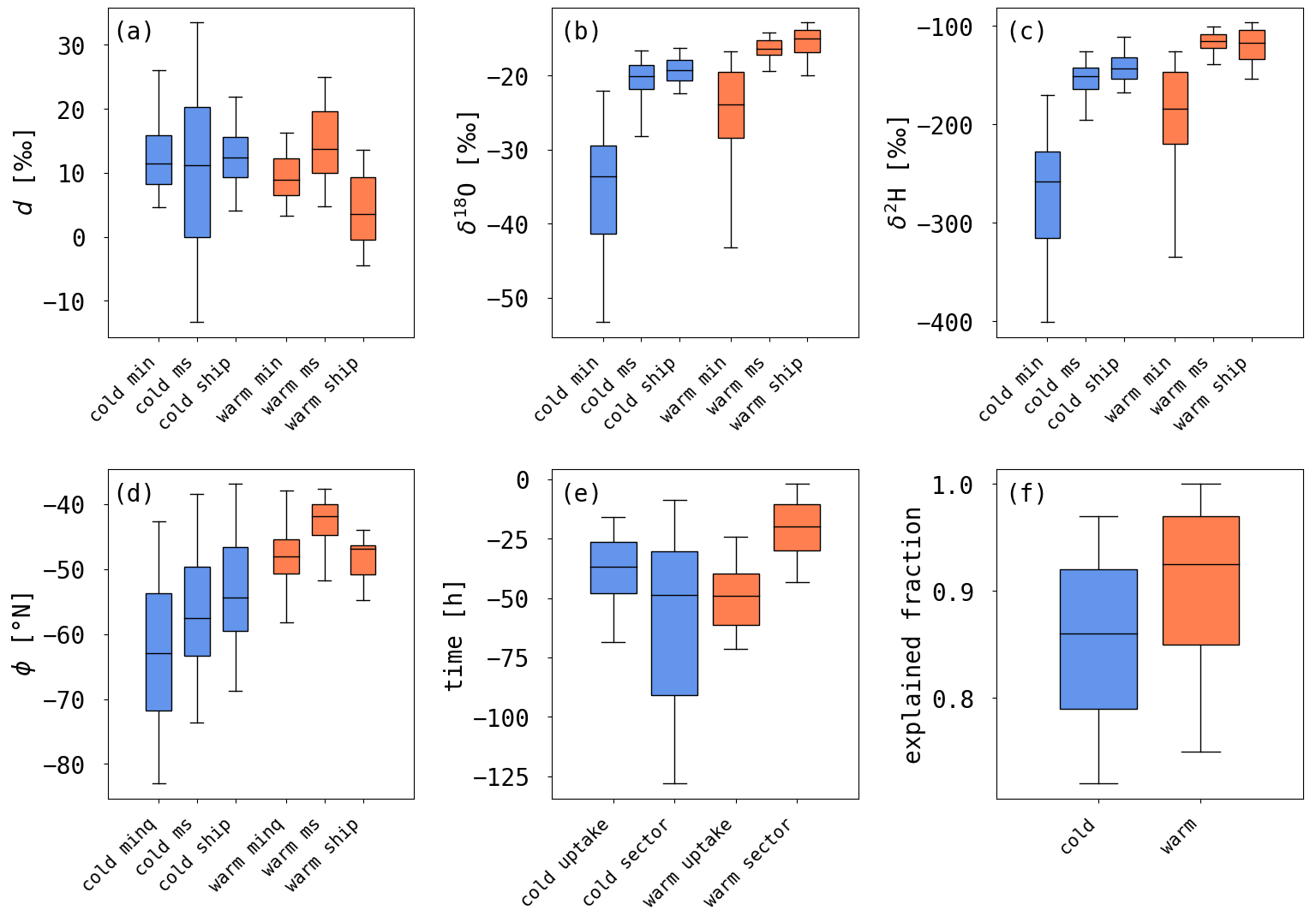
Figure 10Box plots with information derived from COSMOiso trajectories for cold (blue) and warm (orange) temperature advection events. Boxes show the median (black horizontal line in box), interquartile range (boxes) and [5, 95] percentile range (whiskers) of (a) d, (b) δ18O, (c) δ2H and (d) latitude ϕ at minimum specific humidity along the trajectories (minq), the moisture source site (ms) and the ship location (ship), (e) the weighted mean moisture uptake time before arrival (uptake) and the entrance time into the cold and warm sectors (sector), and (f) the specific humidity fraction explained by the moisture source attribution.

Figure 11Composites of COSMOiso trajectories showing time series along trajectories from cold (blue) and warm (red) temperature advection events, respectively, of median values of (a) d, (b) δ18O, (c) δ2H, (d) surface evaporation (E), (e) latitude (ϕ), (f) pressure (p), (g) specific humidity (q), (h) the sum of cloud and ice water content (qc+qi), and (i) the sum of rain and snow water content (qr+qs). Cold and warm temperature advection events are only considered over open ocean (no sea ice, land fraction <0.1 in COSMOiso). Shadings denote the [25, 75] percentile range, and vertical lines show the median time step when the trajectories enter the cold (blue line) and the warm sector (red line). Furthermore, median values are shown for trajectories experiencing no surface precipitation upon arrival (total surface precipitation Rtot<0.01 mm h−1; dashed lines) and for those with surface precipitation upon arrival (Rtot>0.01 mm h−1; dotted lines).
(b) Temporal evolution of SWI signals along cold advection trajectories
The temporal evolution of the median d, δ18O and δ2H along the backward trajectories in the cold sector shows a continuous increase (Fig. 11a–c). These changes occur simultaneously with an increase in ocean evaporation, an equatorward movement and descent of the air (Fig. 11d–f). The strongest changes in d can be observed in the cold sector during the last 48 h before arrival, when the air masses are closest to the ocean surface and the ocean evaporation and specific humidity increase strongly (Fig. 11d, g). The changes of the isotopic composition along the trajectories can be described by two stages. During the first stage, only δ2H and δ18O increase and d stays constant. In this period until approximately 40 h before arrival, the increase in the δ values might be mainly caused by mixing during the descent with air masses at lower altitudes with higher δ values and a similar d as the descending air masses, which does not affect d but leads to an increase in δ18O and δ2H. The second stage starts once the trajectories are closer to the sea surface and within the cold sector, where E and d increase strongly. During this second stage, the air masses are more strongly influenced by ocean evaporation and, thus, non-equilibrium fractionation, which leads to an increase in δ18O and δ2H as well as d. In addition to ocean evaporation, precipitation-related processes such rain evaporation, cloud formation or the equilibration of rain droplets with the surrounding water vapour might affect the isotopic composition of water vapour (Risi et al., 2010a; Aemisegger et al., 2015; Graf et al., 2019). To analyse the effect of precipitation on the water vapour isotopic composition of the air parcels, the median properties along precipitating (surface precipitation >0.01 mm h−1) and non-precipitating (surface precipitation ≤0.01 mm h−1) trajectories upon arrival are calculated based on the simulated surface precipitation in COSMOiso. The air masses arriving in the cold sector are weakly influenced by cloud and precipitation-related processes (Fig. 11h and i, and compare dashed and dotted blue lines in Fig. 11a–i). Precipitating air parcels arriving during cold temperature advection upon arrival have a lower d, higher δ values and a lower pressure, which decreases upon arrival, compared to non-precipitating cold temperature advection trajectories. Overall, the difference between the precipitating and non-precipitating trajectories in the cold sector is small and lies within the [25, 75] percentile range for all variables in Fig. 11. Therefore, the positive anomalies in d due to ocean evaporation in the cold sector are not substantially altered by precipitation-induced changes in the isotopic composition of the MBL water vapour.
The small difference between precipitating and non-precipitating cold temperature advection events can also be observed in the vertical SWI profiles along the ACE ship track, which show a slightly lower d and higher δ values during precipitating than non-precipitating events throughout the MBL (Fig. 12a–c). Over all cold temperature advection events, the equivalent potential temperature (θe) within the MBL indicates well-mixed conditions (Fig. 12d) and a strong influence of ocean evaporation on the MBL moisture budget. This is reflected in the SWI profiles which show constant values in d, δ18O and δ2H in the lower MBL. In the upper MBL, δ18O and δ2H show a weak decrease, which progresses further above the MBL height, implicating vertical mixing of free tropospheric air into the MBL. Even though ocean evaporation is the main process affecting the MBL isotopic composition, cloud processes might affect the region around the MBL top, where d has its minimum values. This minimum occurs above the region of highest cloud and ice water content (qc+qi, Fig. 12e) and rain and snow water content (qr+qs, Fig. 12f). A minimum of d at the MBL top has been observed in measurements of SWIs, and several processes where discussed, such as evaporation of cloud and rain droplets (Sodemann et al., 2017; Salmon et al., 2019). A further process which could induce low d in water vapour close to the MBL top is cloud formation during decreasing temperatures such as during a moist adiabatic ascent. The condensation of water vapour in an environment with decreasing air temperature leads to a decrease in d in the remaining water vapour due to the temperature dependency of equilibrium fractionation (see also Appendix A). More detailed studies of these processes comparing measurements, e.g. aboard aircraft, and model simulations are needed to better understand the processes involved in these low d values at the MBL top.
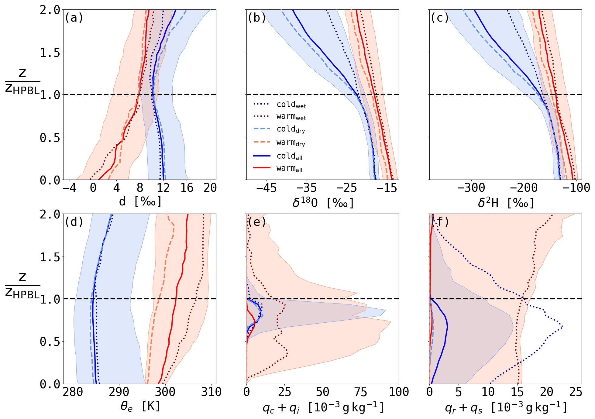
Figure 12Composites of vertical profiles from COSMOiso showing the median of (a) d, (b) δ18O, (c) δ2H, (d) equivalent potential temperature θe, (e) the sum of cloud and ice water content (qc+qi), and (f) the sum of rain and snow water content (qr+qs) for cold (blue) and warm (red) temperature advection events along the ACE ship track. The shading denotes the interquartile range. Furthermore, the median vertical profiles for conditions with (total surface precipitation Rtot>0.01 mm h−1, dotted lines) and without (total surface precipitation Rtot<0.01 mm h−1, dashed lines) surface precipitation are shown for warm and cold temperature advection. On the y axis the height relative to the boundary layer height is shown, where 1 denotes the height of the boundary layer (black dashed line).
(c) Warm temperature advection
For warm temperature advection, the weighted mean moisture uptake occurs 49 [40, 61] h before arrival, while the air parcels enter the warm sector much later at 20 [11, 30] h before arrival (Fig. 10e). Therefore, the air parcels take up moisture upstream of the warm sector of an extratropical cyclone, generally in a region with cold temperature advection and sometimes in a region of zonal flow. Similar to cold temperature advection, the isotopic composition at minimum q along the 7 d backward trajectories with a median value of 3.2 g kg−1 is strongly altered due to ocean evaporation at the moisture source, where the median value of q is 5.8 g kg−1. In contrast to the cold sector, not only δ18O and δ2H, but also d increases from minimum q to the moisture source location. This increase in median d could be caused by a stronger median increase in latitude between minimum q and the moisture source during warm temperature advection compared to cold temperature advection (Fig. 10d). Median d changes by −10 ‰ from the moisture source to arrival, revealing that the isotopic composition of the water vapour can be strongly modified in the warm sector, for example due to cloud formation, precipitation or dew deposition. The strength in d decrease between the moisture source and measurement location depends on the residence time in the warm sector. There is a weak trend (Pearson correlation coefficient ρ=0.31) towards a stronger decrease in d with an increase in residence time in the warm sector (not shown). For a residence time of, for example, 40 h in the warm sector, there is a decrease in d of 11 ‰ between the moisture source and the arrival at the measurement site. During warm temperature advection, the air moves poleward from the moisture source (Fig. 10d and warm temperature advection trajectories in Fig. 4) and shows a weak increase in δ18O from the moisture source to the point of measurement along the ship track. δ2H stays at a similar median value but shows a wider distribution upon arrival compared to the moisture source. Analogously to the cold temperature advection analysis, the temporal evolution of the isotopic composition and other environmental variables along the 4 d backward trajectories are analysed in the following to identify the main process affecting SWIs in the warm sector.
(d) Temporal evolution of SWI signals along warm advection trajectories
For warm temperature advection, δ values increase along the trajectories before the air masses arrive in the warm sector. Within the warm sector, in the last 20 h before arrival, the δ values start to decrease, with δ2H starting earlier than δ18O (Fig. 11b, c). The d already starts decreasing around 60 h before arrival. During the decrease in d outside of the warm sector, the air masses descend and ocean evaporation decreases, while there is only a small increase in q (Fig. 11f, g). Furthermore, the movement of the air masses changes from equatorward to poleward (Fig. 11e). Therefore, this episode of decreasing d outside of the warm sector could be due to weaker non-equilibrium fractionation during ocean evaporation. During the d decrease within the warm sector, the air parcels stay at the same altitude or ascend slightly, while E is close to zero or changes sign, implying dew formation. The median precipitation, which consists of rainfall for 98 % of all precipitation events, and cloud and ice water content increase shortly before arrival of the warm temperature advection trajectories. The evolution of d and the δ values shows that two different processes can lead to the observed decrease in d in the warm sector. After the entrance into the warm sector, d and E decrease, while δ18O and δ2H increase. This stage is dominated by dew deposition, and non-equilibrium processes during dew deposition might lead to the observed changes in SWIs. Shortly before arrival, δ18O and δ2H also start decreasing. At this stage, dew deposition and the interaction of water vapour with cloud and rain droplets affect the isotopic composition of the water vapour. d in cloud droplets is low during the precipitation events in the warm sector (not shown). Therefore, an exchange between cloud droplets and the surrounding water vapour could lead to a decrease in d. Nonetheless, the vertical profiles during warm temperature advection along the ACE track do not show lower d in regions of high qc+qi (Fig. 12a, e). The median vertical d profile and the profile for precipitating and non-precipitating events show the lowest d close to the surface, implying that surface-related processes such as dew deposition are most important in forming negative d anomalies in the warm sector. To better understand the changes in SWIs in the warm sector, the temporal evolution of SWIs in water vapour during the moist processes in the warm sector needs to be described using a mechanistic physical approach. A study is in preparation describing the temporal evolution of the isotopic composition of water vapour with single physical process models.
Even though dew deposition is the most important process in the lower MBL leading to the decrease in d during warm temperature advection, further processes might be important in the upper MBL. The median values along the precipitating and non-precipitating trajectories show small differences to the median values along all trajectories. There are lower d values in the warm sector for precipitating than for non-precipitating trajectories, which are in accordance with lower E along the precipitating trajectories. Nonetheless, these differences lie within the [25, 75] percentile range for all variables in Fig. 11a–g, implying that precipitation upon arrival has a small impact on the SWI evolution of air parcels in the warm sector. A specific difference can be observed for precipitating and non-precipitating air masses in the vertical profiles. The non-precipitating profiles show a minima of d close to the surface and a stagnation in d increase with height in the upper MBL (Fig. 12a). The minimum close to the surface is most likely related to dew deposition similar to the precipitating trajectories. The stagnation in the upper MBL does not correspond to a region of enhanced precipitation or cloud occurrences upon arrival. Therefore, this weaker increase in d in the upper MBL might have been caused by upstream processes as for example the moist adiabatic ascent of the air parcel and subsequent cloud formation similar to the d minimum at the MBL top in the cold sector. Due to the diverse Lagrangian history of the different warm temperature advection events, detailed case studies are needed to study such upstream processes and to understand how important the advection of low d signals in the upper MBL is.
In summary, the analysis of the isotopic composition during cold and warm temperature advection in COSMOiso simulations shows that ocean evaporation and dew deposition are the main processes affecting SWIs in water vapour in the MBL over the Southern Ocean. The impact of local precipitation on the SWIs in the MBL is small compared to the anomalies induced by air–sea interactions. Still, negative d anomalies can be seen in the upper MBL and might be caused by cloud and precipitation-related processes. The ACE measurements confirmed that the SWI signals in the lower MBL along the ACE ship track were adequately simulated in COSMOiso but cannot be used to verify the Lagrangian analysis. The importance of the described processes, such as cloud formation and below-cloud processes, during moisture transport needs more detailed future studies which include the comparison of measurements and model data in the upper MBL and campaigns including upstream measurements of the air mass properties.
The aim of this study was to systematically quantify the contrasting isotopic composition in MBL water vapour in the cold and warm sectors of extratropical cyclones in the Southern Ocean and to identify the main processes that are responsible for these signals. In order to address these objectives in a robust way, i.e. by averaging over many cold and warm sectors, the following prerequisites were indispensable: (i) a method to objectively identify cold and warm sectors of extratropical cyclones that can be applied to ship measurements as well as to reanalysis data (here we used a simple approach focusing on air–sea temperature differences due to cold and warm temperature advection, respectively; Hartmuth, 2019); (ii) an extended data set of SWI measurements available from the 3-month Antarctic Circumnavigation Experiment in 2016/2017 (Thurnherr et al., 2020a), which contains observations from 29 cold and 18 warm advection events corresponding to 462 and 238 h of data, respectively; and (iii) simulations with the high-resolution, SWI-enabled numerical weather prediction model COSMOiso, which allows for the calculation of air parcel trajectories and studying the processes affecting SWI signals along the flow (Pfahl et al., 2012). The simulated SWI signals agree well with the ship-based measurements, in particular, in terms of the observed variability in δ18O, δ2H and d at the synoptic timescale, enabling the joint analysis of observations and simulations. Only the combination of these diagnostic, observational and modelling elements made it possible to provide a portrayal of the characteristic SWI signals associated with warm and cold temperature advection events and their underlying physical processes.
The analyses in this study show that the cold and warm sectors of extratropical cyclones are associated with contrasting isotopic signals in MBL water vapour. The main conclusions can be summarised as follows, separately for situations with cold and warm temperature advection, i.e. for cold and warm sectors of extratropical cyclones, respectively.
-
In the cold sector, negative δ18O and δ2H anomalies (i.e. deviations from the campaign mean) and positive d anomalies occurred together with low hs and a deep and unstable MBL. The trajectory analysis based on COSMOiso simulations showed that during cold temperature advection, the moisture uptake due to ocean evaporation occurs typically 26−48 h before arrival of the considered air parcels at the measurement site. This moisture originates from ocean evaporation mainly within the cold sector itself, and ocean evaporation is the main process that shapes the isotopic composition of the measured water vapour. Moreover, ocean evaporation in the cold sector influences the SWI composition of the entire MBL, leading to an increased vertical gradient of δ2H and δ18O between the MBL and the free troposphere.
-
In the warm sector, positive δ18O and δ2H anomalies and negative d anomalies were observed during meteorological conditions with high hs and a shallow and stable MBL. Processes shaping the SWI composition during warm temperature advection as identified using COSMOiso simulations are more diverse than during cold temperature advection. The air parcels enter the warm sector typically 11–30 h before arrival at the measurement site, which generally occurs after the moisture uptake that is most prominent in the time window 40–61 h before arrival. Therefore, the uptake of moisture that ends in the warm sector happens outside of the warm sector in a region of cold temperature advection and affects the isotopic composition of the air parcels with an increase in δ2H, δ18O and d. In addition, within the warm sector, the air parcels encounter a net loss of moisture due to two main processes. First, air–sea interactions in the form of dew deposition lead to a negative d anomaly and positive δ18O and δ2H anomalies. Second, the formation of clouds and precipitation in ascending air parcels decreases d in water vapour. Thus, in summary, the characteristic SWI signals associated with the warm sector are shaped by both the processes during moisture uptake outside the warm sector, in a context of cold advection, and subsequent dew and cloud formation within the warm sector.
So far, only few studies have discussed the occurrence of low d in MBL water vapour on synoptic timescales. Kurita et al. (2016) analysed SWI measurements in MBL water vapour along the East Antarctic coast. They showed similar contrasting SWI signals over the open ocean as observed in this study with low or negative d and high δ2H in poleward-moving warm air and high d and low δ2H in equatorward-moving air of Antarctic origin. Furthermore, they showed that the δ2H variability along the East Antarctic coast is linked to the southward movement of cyclones, which advect warm and moist air towards the Antarctic continent, potentially contributing to heavy precipitation (Gorodetskaya et al., 2014; Welker et al., 2014). We showed here that these contrasting SWI signals cannot only be found close to Antarctica but throughout the Southern Ocean and that, over the open ocean, the synoptic timescale variability of SWI signals is the result of strongly varying air–sea interactions induced by the meridional advection of air masses within extratropical cyclones. The contrasting air–sea fluxes in cold and warm sectors of extratropical cyclones have been observed in previous ship measurement campaigns, i.e. during pre-ERICA (Neiman et al., 1990) and FASTEX (Persson et al., 2005) in the North Atlantic.
Low or negative d in the boundary layer water vapour has also been observed over ice-covered areas due to the deposition of water vapour on the snow surface (Bonne et al., 2019), where it can impact the isotopic composition of the surface snow (Steen-Larsen et al., 2014a; Casado et al., 2018; Madsen et al., 2019). The here observed d anomalies in the MBL over the open ocean due to air–sea interactions during warm and cold temperature advection could also lead to changes in the isotopic composition of the ocean surface waters or, even more prominently, precipitation formed from these air masses. It is an important implication of the results in this study that clouds forming in the cold sector of extratropical cyclones (typically shallow convective cloud) and clouds forming in the warm sector (typically in the rapidly, slant-wise-ascending warm conveyor belts) rely on different SWI starting conditions, i.e. on vapour with contrasting SWI anomalies. A recent study (Aemisegger, 2018) found a clear link between d in monthly precipitation in Reykjavik (Iceland) and the frequency and location of North Atlantic cyclones, which influences the location of strong ocean evaporation during cold temperature advection. It has yet to be studied if and how air–sea fluxes in the context of warm temperature advection affect the isotopic composition of precipitation, for example, in warm conveyor belts. Future collocated measurements of dew and fog over the ocean during warm advection events will provide key insights into the coupling between clouds and their environments. Previous studies over land showed that the time evolution of the isotopic composition of cloud droplets in fog was mainly driven by the moisture origin at large scales and the enrichment of the fog dependent on the occurrence of precipitation within the cloud (Spiegel et al., 2012a, b). Future detailed studies of simultaneous cloud water, vapour, precipitation and dew over the ocean within near-surface clouds would provide important empirical data for the validation of model isotope microphysics.
A previous, highly idealised study based on COSMOiso simulations without isotopic fractionation during ocean evaporation (Dütsch et al., 2016) has shown that δ2H in the cold and warm sectors of extratropical cyclones is primarily affected by horizontal transport. Here, we confirm that the meridional large-scale transport of air strongly affects the isotopic composition of the MBL water vapour, based on observations and real-case simulations. In particular, δ18O and δ2H in water vapour in the cold and warm sectors of extratropical cyclones are influenced by ocean evaporation at the moisture source. The moisture uptake over the ocean surface leads to an increase in δ18O and δ2H, and this SWI signal is only marginally changed during transport to the measurement site. Surprisingly, and in contrast to δ18O and δ2H, d shows large variations after the moisture uptake in the warm sector, indicating that d in the warm sector is not only influenced by the moisture source conditions but is changed substantially during transport. Therefore, the isotopic composition of water vapour in the MBL is mainly a signal from air–sea interactions, such as ocean evaporation at the moisture source in the cold sector and dew deposition during transport in the warm sector. The mechanisms leading to isotopic fractionation associated with ocean evaporation, dew deposition, and cloud formation as well as the relative contributions of these processes to the observed SWI variability in the cold and warm sector of extratropical cyclones will be analysed in future studies. Furthermore, the findings of this study are valuable for further studies analysing meridional air mass advection and other characteristics associated with the dynamics of the storm tracks over interannual timescales.
The condensation of water vapour in an ascending air parcel leads to the formation of cloud droplets and changes the isotopic composition of the remaining atmospheric water vapour. This process can be modelled using a Rayleigh fractionation model based on the temperature and moisture evolution of a moist adiabatic ascent of an air parcel. Thereby it is assumed that the condensed cloud droplets do not interact anymore with the surrounding water vapour after condensation and are immediately removed. This is a simplification of processes occurring during cloud formation, but it provides a first-order understanding of isotopic variations due to cloud formation.
A Rayleigh model (Dansgaard, 1964) is used to estimate the effect of condensation during a moist adiabatic ascent on the isotopic composition of water vapour, including the temperature dependency of the equilibrium fractionation factor αe(T) (Horita and Wesolowski, 1994) and the transition from liquid to ice clouds as in Dütsch et al. (2017). An effective isotopic fractionation factor αeff>1 is defined, depending on temperature and the relative fractions of liquid and solid condensate during the moist adiabatic ascent: . fliq is 0 for T<250.15 K and 1 for T>273.15 K, and a quadratic interpolation is used in between these temperatures to represent mixed-phase clouds. αice>1 is the equilibrium fractionation factor in vapour with respect to ice (Majoube, 1971), adjusted for supersaturation over ice (Jouzel and Merlivat, 1984).
Figure A1 shows the Rayleigh fractionation during a moist adiabatic ascent, which is initiated at a temperature of 283.15 K, a pressure of 1000 hPa, and isotopic compositions ‰ and ‰ (which corresponds to d0=6 ‰). Four different scenarios are calculated:
-
Rayleigh fractionation with constant temperature and a stepwise loss of moisture (blue line).
-
Rayleigh fractionation along a moist adiabatic ascent, i.e. with temperature variations, assuming only liquid clouds (black line).
-
Same as 2 but including ice cloud formation and the fractionation factor for vapour over ice (green line).
-
Same as 3 but including an adjustment of the ice fractionation factor due to ice supersaturation (orange line).
All of these four scenarios show a depletion of δ18O and δ2H in water vapour with ongoing moisture loss. d in water vapour decreases in the beginning for all scenarios. The decrease in d is small with a value around 1 ‰ for scenario 1 with constant temperature and increases to values above the start value after the condensation of 75 % of the humidity. In the other three scenarios, there is a stronger decrease in d with minimum values of more than 6 ‰ below the starting value. This stronger decrease in d is due to the temperature dependency of the equilibrium fractionation factor, which increases more rapidly with decreasing temperature for 2H than for 18O (see 2αeff(18αeff)−1 in Fig. A1d). Thus, d in the remaining vapour decreases with decreasing temperature. Scenario 3, which includes the equilibrium fractionation effects of the ice phase but neglects non-equilibrium effects due to supersaturation, shows a weaker decrease in d. When including ice supersaturation, the evolution of d follows a similar pattern as scenario 2 with only liquid cloud formation. Once the amount of heavy isotopes in the vapour phase becomes very small, d increases by definition (due to the non-linearity of the δ scale; see also Dütsch et al., 2017) for all scenarios. These four scenarios show that Rayleigh fractionation during a moist adiabatic ascent can lead to a substantial decrease in d in water vapour.
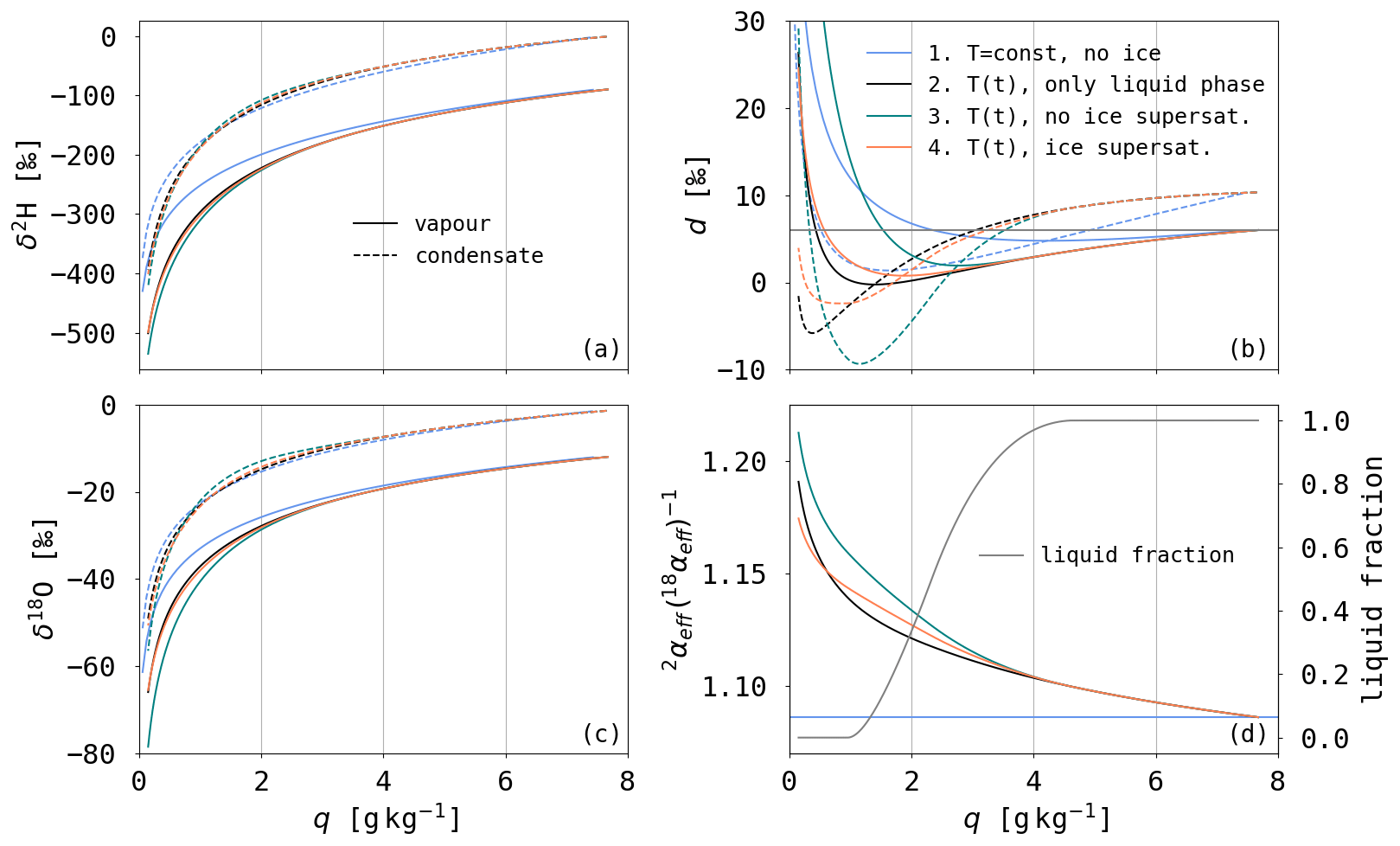
Figure A1Modelled (a) δ2H, (b) d and (c) δ18O of water vapour (solid lines) and condensate (dashed lines) versus specific humidity q during Rayleigh fractionation with different model setups (see text for details). Furthermore, the ratio of 2αeff and 18αeff for each model setup as a function of q and the liquid fraction for the two setups with ice cloud formation is shown in panel (d).
The ACE data sets are published on the research data repository zenodo: https://zenodo.org/communities/spi-ace/ (Thomas, 2021). The radiosonde data set is accessible with the DOI https://doi.org/10.5281/zenodo.4382460 (Gorodetskaya et al., 2021) and the rainfall data set with the DOI https://doi.org/10.5281/zenodo.3929289 (Gehring et al., 2020). The COSMOiso simulations are published on the ETH research collection with the DOI https://doi.org/10.3929/ethz-b-000445744 (Thurnherr et al., 2020b). The snowfall data set is available upon request (irina.gorodetskaya@ua.pt).
The supplement related to this article is available online at: https://doi.org/10.5194/wcd-2-331-2021-supplement.
HW, FA and IT initiated the project. IT, MB, FA and HW discussed the day-to-day large-scale meteorology during and after the ACE campaign based on forecast and analysis weather charts prepared by MB. IT performed the analyses and produced the figures. KH developed and evaluated the temperature advection diagnostic during her master's thesis, with contributions from IT and FA. MW provided the ECHAM5-wiso global boundary data for the regional COSMOiso simulations. FA, LJ and IT designed and prepared the setup for the COSMOiso simulations performed during LJ's master's thesis by LJ and IT at the Swiss National Supercomputing Centre (CSCS). IG, FA and IT contributed to the production of the radiosonde data set. JG produced the rainfall data and IG the snowfall data. IT wrote the paper, supported by FA and HW. All co-authors provided feedback on the manuscript.
The authors declare that they have no conflict of interest.
ACE was a scientific expedition carried out under the auspices of the Swiss Polar Institute, supported by funding from the ACE Foundation and Ferring Pharmaceuticals. The COSMOiso simulations were performed at the Swiss National Supercomputing Centre (CSCS) with the small production projects sm08 and sm32. The authors acknowledge MeteoSwiss and ECMWF for the access to the ERA-Interim reanalyses and operational forecasts. We thank F. Martin Ralph for co-funding the ACE radio soundings, Pascal Graf for his help during the planning of the sounding equipment and design, and the ACE team for the helping hands during the launchings. We thank the anonymous reviewers for their constructive comments that helped to improve the paper.
This research has been supported by the ACE Foundation, Ferring Pharmaceuticals and the BNP Paribas Foundation (grant nos. ACE project 11 and ACE project 18); the Swiss National Science Foundation (grant nos. PZ00P2_142684, 175700/1 and 165941); the European Research Council, H2020 research and innovation programme (INTEXseas, grant no. 787652); and the FCT/MCTES (CESAM, grant nos. UIDP/50017/2020 and UIDB/50017/2020; FCT project ATLACE, CIRCNA/CAC/0273/2019 grant).
This paper was edited by Helen Dacre and reviewed by three anonymous referees.
Aemisegger, F.: On the link between the North Atlantic storm track and precipitation deuterium excess in Reykjavik, Atmos. Sci. Lett., 19, e865, https://doi.org/10.1002/asl.865, 2018. a
Aemisegger, F. and Papritz, L.: A climatology of strong large-scale ocean evaporation events, Part I: Identification, global distribution, and associated climate conditions, J. Climate, 31, 7287–7312, https://doi.org/10.1175/JCLI-D-17-0591.1, 2018. a, b, c, d
Aemisegger, F. and Sjolte, J.: A climatology of strong large-scale ocean evaporation events, Part II: Relevance for the deuterium excess signature of the evaporation flux, J. Climate, 31, 7313–7336, https://doi.org/10.1175/JCLI-D-17-0592.1, 2018. a, b
Aemisegger, F., Pfahl, S., Sodemann, H., Lehner, I., Seneviratne, S. I., and Wernli, H.: Deuterium excess as a proxy for continental moisture recycling and plant transpiration, Atmos. Chem. Phys., 14, 4029–4054, https://doi.org/10.5194/acp-14-4029-2014, 2014. a
Aemisegger, F., Spiegel, J. K., Pfahl, S., Sodemann, H., Eugster, W., and Wernli, H.: Isotope meteorology of cold front passages: A case study combining observations and modeling: Water isotopes during cold fronts, Geophys. Res. Lett., 42, 5652–5660, https://doi.org/10.1002/2015GL063988, 2015. a, b, c
Beare, R. J.: Boundary layer mechanisms in extratropical cyclones, Q. J. Roy. Meteor. Soc., 133, 503–515, https://doi.org/10.1002/qj.30, 2007. a, b, c
Benetti, M., Aloisi, G., Reverdin, G., Risi, C., and Sèze, G.: Importance of boundary layer mixing for the isotopic composition of surface vapor over the subtropical North Atlantic Ocean, J. Geophys. Res.-Atmos., 120, 2190–2209, https://doi.org/10.1002/2014JD021947, 2015. a
Bharti, V., Fairall, C. W., Blomquist, B. W., Huang, Y., Protat, A., Sullivan, P. P., Siems, S. T., and Manton, M. J.: Air-sea heat and momentum fluxes in the Southern Ocean, J. Geophys. Res.-Atmos., 124, 12426–12443, https://doi.org/10.1029/2018JD029761, 2019. a, b
Blossey, P. N., Kuang, Z., and Romps, D. M.: Isotopic composition of water in the tropical tropopause layer in cloud-resolving simulations of an idealized tropical circulation, J. Geophys. Res.-Atmos., 115, D24309, https://doi.org/10.1029/2010JD014554, 2010. a
Bond, N. A. and Fleagle, R. G.: Prefrontal and postfrontal boundary layer processes over the ocean, Mon. Weather Rev., 116, 1257–1273, https://doi.org/10.1175/1520-0493(1988)116<1257:PAPBLP>2.0.CO;2, 1988. a
Bonne, J.-L., Behrens, M., Meyer, H., Kipfstuhl, S., Rabe, B., Schönicke, L., Steen-Larsen, H. C., and Werner, M.: Resolving the controls of water vapour isotopes in the Atlantic sector, Nat. Commun., 10, 1632, https://doi.org/10.1038/s41467-019-09242-6, 2019. a, b, c, d, e
Boutle, I. A., Beare, R. J., Belcher, S. E., Brown, A. R., and Plant, R. S.: The moist boundary layer under a mid-latitude weather system, Bound.-Lay. Meteorol., 134, 367–386, https://doi.org/10.1007/s10546-009-9452-9, 2010. a, b
Boutle, I. A., Belcher, S. E., and Plant, R. S.: Moisture transport in midlatitude cyclones, Q. J. Roy. Meteor. Soc., 137, 360–373, https://doi.org/10.1002/qj.783, 2011. a
Browning, K. A.: Organization of Clouds and Precipitation in Extratropical Cyclones, in: Extratropical Cyclones: The Erik Palmén Memorial Volume, American Meteorological Society, Boston, Massachusetts, 129–153, https://doi.org/10.1007/978-1-944970-33-8_8, 1990. a
Butzin, M., Werner, M., Masson-Delmotte, V., Risi, C., Frankenberg, C., Gribanov, K., Jouzel, J., and Zakharov, V. I.: Variations of oxygen-18 in West Siberian precipitation during the last 50 years, Atmos. Chem. Phys., 14, 5853–5869, https://doi.org/10.5194/acp-14-5853-2014, 2014. a
Casado, M., Landais, A., Picard, G., Münch, T., Laepple, T., Stenni, B., Dreossi, G., Ekaykin, A., Arnaud, L., Genthon, C., Touzeau, A., Masson-Delmotte, V., and Jouzel, J.: Archival processes of the water stable isotope signal in East Antarctic ice cores, The Cryosphere, 12, 1745–1766, https://doi.org/10.5194/tc-12-1745-2018, 2018. a
Catto, J. L., Jakob, C., Berry, G., and Nicholls, N.: Relating global precipitation to atmospheric fronts, Geophys. Res. Lett., 39, L10805, https://doi.org/10.1029/2012GL051736, 2012. a
Chen, S., Campbell, T. J., Jin, H., Gaberšek, S., Hodur, R. M., and Martin, P.: Effect of two-way air-sea coupling in high and low wind speed regimes, Mon. Weather Rev., 138, 3579–3602, https://doi.org/10.1175/2009MWR3119.1, 2010. a
Christner, E., Aemisegger, F., Pfahl, S., Werner, M., Cauquoin, A., Schneider, M., Hase, F., Barthlott, S., and Schädler, G.: The climatological impacts of continental surface evaporation, rainout, and subcloud processes on δD of water vapor and precipitation in Europe, J. Geophys. Res.-Atmos., 123, 4390–4409, https://doi.org/10.1002/2017JD027260, 2018. a, b
Condron, A. and Renfrew, I. A.: The impact of polar mesoscale storms on northeast Atlantic Ocean circulation, Nat. Geosci., 6, 34–37, https://doi.org/10.1038/ngeo1661, 2013. a
Condron, A., Bigg, G. R., and Renfrew, I. A.: Polar mesoscale cyclones in the northeast Atlantic: Comparing climatologies from ERA-40 and satellite imagery, Mon. Weather Rev., 134, 1518–1533, https://doi.org/10.1175/MWR3136.1, 2006. a
Craig, H. and Gordon, L. I.: Deuterium and oxygen 18 variations in the ocean and the marine atmosphere, in: Stable Isotopes in Oceanographic Studies and Paleotemperatures, edited by: Tongiorgi, E., 9–130, Lab. Geol. Nucl., Pisa, Italy, 1965. a
Dansgaard, W.: Stable isotopes in precipitation, Tellus, 16, 436–468, https://doi.org/10.3402/tellusa.v16i4.8993, 1964. a, b
Dee, D. P., Uppala, S. M., Simmons, A. J., Berrisford, P., Poli, P., Kobayashi, S., Andrae, U., Balmaseda, M. A., Balsamo, G., Bauer, P., Bechtold, P., Beljaars, A. C. M., van de Berg, L., Bidlot, J., Bormann, N., Delsol, C., Dragani, R., Fuentes, M., Geer, A. J., Haimberger, L., Healy, S. B., Hersbach, H., Hólm, E. V., Isaksen, L., Kållberg, P., Köhler, M., Matricardi, M., McNally, A. P., Monge-Sanz, B. M., Morcrette, J.-J., Park, B.-K., Peubey, C., de Rosnay, P., Tavolato, C., Thépaut, J.-N., and Vitart, F.: The ERA-Interim reanalysis: configuration and performance of the data assimilation system, Q. J. Roy. Meteor. Soc., 137, 553–597, https://doi.org/10.1002/qj.828, 2011. a, b
Doms, G., Förstner, J., Heise, E., Herzog, H.-J., Mironov, D., Raschendorfer, M., Reinhardt, T., Ritter, B., Schrodin, R., Schulz, J.-P., and Vogel, G.: A description of the nonhydrostatic regional COSMO model, Part II: Physical parameterization, Deutscher Wetterdienst, Offenbach, Germany, 2013. a
Dütsch, M., Pfahl, S., and Wernli, H.: Drivers of δ2H variations in an idealized extratropical cyclone, Geophys. Res. Lett., 43, 5401–5408, https://doi.org/10.1002/2016GL068600, 2016. a, b
Dütsch, M., Pfahl, S., and Sodemann, H.: The impact of nonequilibrium and equilibrium fractionation on two different deuterium excess definitions, J. Geophys. Res.-Atmos., 122, 12732–12746, https://doi.org/10.1002/2017JD027085, 2017. a, b
Dütsch, M., Pfahl, S., Meyer, M., and Wernli, H.: Lagrangian process attribution of isotopic variations in near-surface water vapour in a 30-year regional climate simulation over Europe, Atmos. Chem. Phys., 18, 1653–1669, https://doi.org/10.5194/acp-18-1653-2018, 2018. a, b
Fleagle, R. G. and Nuss, W. A.: The distribution of surface fluxes and boundary layer divergence in midlatitude ocean storms, J. Atmos. Sci., 42, 784–799, https://doi.org/10.1175/1520-0469(1985)042<0784:TDOSFA>2.0.CO;2, 1985. a, b
Gat, J. R.: The isotopic composition of evaporating waters – review of the historical evolution leading up to the Craig-Gordon model, Isot. Environ. Healt. S., 44, 5–9, https://doi.org/10.1080/10256010801887067, 2008. a
Gat, J. R., Klein, B., Kushnir, Y., Roether, W., Wernli, H., Yam, R., and Shemesh, A.: Isotope composition of air moisture over the Mediterranean Sea: An index of the air-sea interaction pattern, Tellus B, 55, 953–965, https://doi.org/10.1034/j.1600-0889.2003.00081.x, 2003. a
Gehring, J., Thurnherr, I., and Graf, P.: Vertical profiles of Doppler spectra of hydrometeors from a Micro Rain Radar recorded during the austral summer of 2016/2017 in the Southern Ocean on the Antarctic Circumnavigation Expedition (ACE) [Data set], Zenodo, https://doi.org/10.5281/zenodo.3929289, 2020. a, b
Gorodetskaya, I. V., Tsukernik, M., Claes, K., Ralph, M. F., Neff, W. D., and Van Lipzig, N. P. M.: The role of atmospheric rivers in anomalous snow accumulation in East Antarctica, Geophys. Res. Lett., 41, 6199–6206, https://doi.org/10.1002/2014GL060881, 2014. a
Gorodetskaya, I. V., Thurnherr, I., Tsukernik, M., Graf, P., Aemisegger, F., Wernli, H., and Ralph, F. M.: Atmospheric profiling data collected from radiosondes in the Southern Ocean in the austral summer of 2016/2017 during the Antarctic Circumnavigation Expedition. (Version 1.0) [Data set], Zenodo, https://doi.org/10.5281/zenodo.4382460, 2021. a, b
Graf, P., Wernli, H., Pfahl, S., and Sodemann, H.: A new interpretative framework for below-cloud effects on stable water isotopes in vapour and rain, Atmos. Chem. Phys., 19, 747–765, https://doi.org/10.5194/acp-19-747-2019, 2019. a
Grazioli, J., Genthon, C., Boudevillain, B., Duran-Alarcon, C., Del Guasta, M., Madeleine, J.-B., and Berne, A.: Measurements of precipitation in Dumont d'Urville, Adélie Land, East Antarctica, The Cryosphere, 11, 1797–1811, https://doi.org/10.5194/tc-11-1797-2017, 2017. a
Hartmuth, K.: The role of cold and warm air advection for the hydrological cycle in the South Indian Ocean, Master's thesis, ETH Zurich, Zurich, Switzerland, https://doi.org/10.3929/ethz-b-000437864, 2019. a, b
Haumann, F. A., Robinson, C., Thomas, J., Hutchings, J., Pina Estany, C., Tarasenko, A., Gerber, F., and Leonard, K.: Physical and biogeochemical oceanography data from underway measurements with an AquaLine Ferrybox during the Antarctic Circumnavigation Expedition (ACE) [Data set], Zenodo, https://doi.org/10.5281/zenodo.3660852, 2020. a
Hewson, T. D.: Objective fronts, Meteorol. Appl., 5, 37–65, https://doi.org/10.1017/S1350482798000553, 1998. a
Holt, T. and Raman, S.: Marine boundary-layer structure and circulation in the region of offshore redevelopment of a cyclone during GALE, Mon. Weather Rev., 118, 392–410, https://doi.org/10.1175/1520-0493(1990)118<0392:MBLSAC>2.0.CO;2, 1990. a
Horita, J. and Wesolowski, D. J.: Liquid-vapor fractionation of oxygen and hydrogen isotopes of water from the freezing to the critical temperature, Geochim. Cosmochim. Ac., 58, 3425–3437, https://doi.org/10.1016/0016-7037(94)90096-5, 1994. a
Jansing, L.: Marine boundary layer stable water isotope variability in the Southern Ocean – An investigation using the regional COSMOiso model, Master's thesis, ETH Zurich, Zurich, Switzerland, https://doi.org/10.3929/ethz-b-000438068, 2019. a, b, c
Jenkner, J., Sprenger, M., Schwenk, I., Schwierz, C., Dierer, S., and Leuenberger, D.: Detection and climatology of fronts in a high-resolution model reanalysis over the Alps, Meteorol. Appl., 17, 1–18, https://doi.org/10.1002/met.142, 2010. a
Joussaume, S., Sadourny, R., and Jouzel, J.: A general circulation model of water isotope cycles in the atmosphere, Nature, 311, 24–29, https://doi.org/10.1038/311024a0, 1984. a
Jouzel, J. and Merlivat, L.: Deuterium and oxygen 18 in precipitation: Modeling of the isotopic effects during snow formation, J. Geophys. Res.-Atmos., 89, 11749–11757, https://doi.org/10.1029/JD089iD07p11749, 1984. a
Kurita, N., Hirasawa, N., Koga, S., Matsushita, J., Steen-Larsen, H. C., Masson-Delmotte, V., and Fujiyoshi, Y.: Influence of large-scale atmospheric circulation on marine air intrusion toward the East Antarctic coast, Geophys. Res. Lett., 43, 9298–9305, https://doi.org/10.1002/2016GL070246, 2016. a
Kuwano-Yoshida, A. and Minobe, S.: Storm-track response to SST fronts in the northwestern Pacific region in an AGCM, J. Climate, 30, 1081–1102, https://doi.org/10.1175/JCLI-D-16-0331.1, 2016. a
Lambert, S. J.: A cyclone climatology of the Canadian Climate Centre general circulation model, J. Climate, 1, 109–115, https://doi.org/10.1175/1520-0442(1988)001<0109:ACCOTC>2.0.CO;2, 1988. a
Landwehr, S., Thomas, J., Gorodetskaya, I., Thurnherr, I., Robinson, C., and Schmale, J.: Quality-checked meteorological data from the Southern Ocean collected during the Antarctic Circumnavigation Expedition from December 2016 to April 2017 [Data set], Zenodo, https://doi.org/10.5281/zenodo.3379590, 2019. a
Lee, K.-O., Aemisegger, F., Pfahl, S., Flamant, C., Lacour, J.-L., and Chaboureau, J.-P.: Contrasting stable water isotope signals from convective and large-scale precipitation phases of a heavy precipitation event in southern Italy during HyMeX IOP 13: a modelling perspective, Atmos. Chem. Phys., 19, 7487–7506, https://doi.org/10.5194/acp-19-7487-2019, 2019. a, b
Maahn, M. and Kollias, P.: Improved Micro Rain Radar snow measurements using Doppler spectra post-processing, Atmos. Meas. Tech., 5, 2661–2673, https://doi.org/10.5194/amt-5-2661-2012, 2012. a
Madonna, E., Wernli, H., Joos, H., and Martius, O.: Warm conveyor belts in the ERA-Interim dataset (1979–2010), Part I: Climatology and potential vorticity evolution, J. Climate, 27, 3–26, https://doi.org/10.1175/JCLI-D-12-00720.1, 2014. a
Madsen, M. V., Steen-Larsen, H. C., Hörhold, M., Box, J., Berben, S. M. P., Capron, E., Faber, A.-K., Hubbard, A., Jensen, M. F., Jones, T. R., Kipfstuhl, S., Koldtoft, I., Pillar, H. R., Vaughn, B. H., Vladimirova, D., and Dahl-Jensen, D.: Evidence of Isotopic Fractionation During Vapor Exchange Between the Atmosphere and the Snow Surface in Greenland, J. Geophys. Res.-Atmos., 124, 2932–2945, https://doi.org/10.1029/2018JD029619, 2019. a
Majoube, M.: Fractionnement en oxygene 18 et en deuterium entre l'eau et sa vapeur, J. Chim. Phys., 68, 1423–1436, https://doi.org/10.1051/jcp/1971681423, 1971. a
Merlivat, L. and Jouzel, J.: Global climatic interpretation of the deuterium-oxygen 18 relationship for precipitation, J. Geophys. Res.-Oceans, 84, 5029–5033, https://doi.org/10.1029/JC084iC08p05029, 1979. a, b
Moore, G. W. K. and Renfrew, I. A.: An assessment of the surface turbulent heat fluxes from the NCEP–NCAR reanalysis over the western boundary currents, J. Climate, 15, 2020–2037, https://doi.org/10.1175/1520-0442(2002)015<2020:AAOTST>2.0.CO;2, 2002. a
Moore, J. K., Abbott, M. R., and Richman, J. G.: Location and dynamics of the Antarctic Polar Front from satellite sea surface temperature data, J. Geophys. Res.-Oceans, 104, 3059–3073, https://doi.org/10.1029/1998JC900032, 1999. a
Neiman, P. J., Shapiro, M. A., Donall, E. G., and Kreitzberg, C. W.: Diabatic modification of an extratropical marine cyclone warm sector by cold underlying water, Mon. Weather Rev., 118, 1576–1590, https://doi.org/10.1175/1520-0493(1990)118<1576:DMOAEM>2.0.CO;2, 1990. a, b, c, d
Nicolas, J. P. and Bromwich, D. H.: Precipitation changes in high southern latitudes from global reanalyses: A cautionary tale, Surv. Geophys., 32, 475–494, https://doi.org/10.1007/s10712-011-9114-6, 2011. a, b
Nuss, W. A.: Air-Sea interaction influences on the structure and intensification of an idealized marine cyclone, Mon. Weather Rev., 117, 351–369, https://doi.org/10.1175/1520-0493(1989)117<0351:ASIIOT>2.0.CO;2, 1989. a
Papritz, L., Pfahl, S., Rudeva, I., Simmonds, I., Sodemann, H., and Wernli, H.: The role of extratropical cyclones and fronts for Southern Ocean freshwater fluxes, J. Climate, 27, 6205–6224, https://doi.org/10.1175/JCLI-D-13-00409.1, 2014. a, b
Papritz, L., Pfahl, S., Sodemann, H., and Wernli, H.: A climatology of cold air outbreaks and their impact on air-sea heat fluxes in the high-latitude South Pacific, J. Climate, 28, 342–364, https://doi.org/10.1175/JCLI-D-14-00482.1, 2015. a, b
Persson, P. O. G., Hare, J. E., Fairall, C. W., and Otto, W. D.: Air-sea interaction processes in warm and cold sectors of extratropical cyclonic storms observed during FASTEX, Q. J. Roy. Meteor. Soc., 131, 877–912, https://doi.org/10.1256/qj.03.181, 2005. a, b, c, d
Peters, G., Fischer, B., Münster, H., Clemens, M., and Wagner, A.: Profiles of raindrop size distributions as retrieved by microrain radars, J. Appl. Meteorol., 44, 1930–1949, https://doi.org/10.1175/JAM2316.1, 2005. a
Pfahl, S. and Wernli, H.: Air parcel trajectory analysis of stable isotopes in water vapor in the eastern Mediterranean, J. Geophys. Res., 113, D20104, https://doi.org/10.1029/2008JD009839, 2008. a, b, c, d
Pfahl, S. and Wernli, H.: Lagrangian simulations of stable isotopes in water vapor: An evaluation of nonequilibrium fractionation in the Craig-Gordon model, J. Geophys. Res.-Atmos., 114, D20108, https://doi.org/10.1029/2009JD012054, 2009. a, b, c, d
Pfahl, S., Wernli, H., and Yoshimura, K.: The isotopic composition of precipitation from a winter storm – a case study with the limited-area model COSMOiso, Atmos. Chem. Phys., 12, 1629–1648, https://doi.org/10.5194/acp-12-1629-2012, 2012. a, b, c, d, e, f
Pfahl, S., Madonna, E., Boettcher, M., Joos, H., and Wernli, H.: Warm conveyor belts in the ERA-Interim dataset (1979–2010), Part II: Moisture origin and relevance for precipitation, J. Climate, 27, 27–40, https://doi.org/10.1175/JCLI-D-13-00223.1, 2014. a
Pollard, R. T., Guymer, T. H., Taylor, P. K., Charnock, H., and Pollard, R. T.: Summary of the JASIN 1978 field experiment, Philos. T Roy. Soc. A, 308, 221–230, https://doi.org/10.1098/rsta.1983.0001, 1983. a
Rasmussen, E. A. and Turner, J.: Polar lows: Mesoscale Weather Systems in the Polar Regions, Cambridge University Press, Cambridge, UK, https://doi.org/10.1017/CBO9780511524974, 2003. a
Renfrew, I. A., Pickart, R. S., Våge, K., Moore, G. W. K., Bracegirdle, T. J., Elvidge, A. D., Jeansson, E., Lachlan-Cope, T., McRaven, L. T., Papritz, L., Reuder, J., Sodemann, H., Terpstra, A., Waterman, S., Valdimarsson, H., Weiss, A., Almansi, M., Bahr, F., Brakstad, A., Barrell, C., Brooke, J. K., Brooks, B. J., Brooks, I. M., Brooks, M. E., Bruvik, E. M., Duscha, C., Fer, I., Golid, H. M., Hallerstig, M., Hessevik, I., Huang, J., Houghton, L., Jónsson, S., Jonassen, M., Jackson, K., Kvalsund, K., Kolstad, E. W., Konstali, K., Kristiansen, J., Ladkin, R., Lin, P., Macrander, A., Mitchell, A., Olafsson, H., Pacini, A., Payne, C., Palmason, B., Pérez-Hernández, M. D., Peterson, A. K., Petersen, G. N., Pisareva, M. N., Pope, J. O., Seidl, A., Semper, S., Sergeev, D., Skjelsvik, S., Søiland, H., Smith, D., Spall, M. A., Spengler, T., Touzeau, A., Tupper, G., Weng, Y., Williams, K. D., Yang, X., and Zhou, S.: The Iceland Greenland Seas Project, B. Am. Meteorol. Soc., 100, 1795–1817, https://doi.org/10.1175/BAMS-D-18-0217.1, 2019. a
Reynolds, R. W., Smith, T. M., Liu, C., Chelton, D. B., Casey, K. S., and Schlax, M. G.: Daily high-resolution-blended analyses for sea surface temperature, J. Climate, 20, 5473–5496, https://doi.org/10.1175/2007JCLI1824.1, 2007. a
Risi, C., Bony, S., Vimeux, F., Chong, M., and Descroix, L.: Evolution of the stable water isotopic composition of the rain sampled along Sahelian squall lines, Q. J. Roy. Meteor. Soc., 136, 227–242, https://doi.org/10.1002/qj.485, 2010a. a
Risi, C., Bony, S., Vimeux, F., and Jouzel, J.: Water-stable isotopes in the LMDZ4 general circulation model: Model evaluation for present-day and past climates and applications to climatic interpretations of tropical isotopic records, J. Geophys. Res.-Atmos., 115, D12118, https://doi.org/10.1029/2009JD013255, 2010b. a
Rudeva, I. and Gulev, S. K.: Composite analysis of North Atlantic extratropical cyclones in NCEP–NCAR reanalysis data, Mon. Weather Rev., 139, 1419–1446, https://doi.org/10.1175/2010MWR3294.1, 2010. a
Salmon, O. E., Welp, L. R., Baldwin, M. E., Hajny, K. D., Stirm, B. H., and Shepson, P. B.: Vertical profile observations of water vapor deuterium excess in the lower troposphere, Atmos. Chem. Phys., 19, 11525–11543, https://doi.org/10.5194/acp-19-11525-2019, 2019. a
Schemm, S., Rudeva, I., and Simmonds, I.: Extratropical fronts in the lower troposphere – global perspectives obtained from two automated methods, Q. J. Roy. Meteor. Soc., 141, 1686–1698, https://doi.org/10.1002/qj.2471, 2015. a
Schmale, J., Baccarini, A., Thurnherr, I., Henning, S., Efraim, A., Regayre, L., Bolas, C., Hartmann, M., Welti, A., Lehtipalo, K., Aemisegger, F., Tatzelt, C., Landwehr, S., Modini, R. L., Tummon, F., Johnson, J., Harris, N., Schnaiter, M., Toffoli, A., Derkani, M., Bukowiecki, N., Stratmann, F., Dommen, J., Baltensperger, U., Wernli, H., Rosenfeld, D., Gysel-Beer, M., and Carslaw, K.: Overview of the Antarctic Circumnavigation Expedition: Study of Preindustrial-like Aerosols and their Climate Effects (ACE–SPACE), B. Am. Meteorol. Soc., 100, 2260–2283, https://doi.org/10.1175/BAMS-D-18-0187.1, 2019. a
Sinclair, V. A., Belcher, S. E., and Gray, S. L.: Synoptic controls on boundary-layer characteristics, Bound.-Lay. Meteorol., 134, 387–409, https://doi.org/10.1007/s10546-009-9455-6, 2010. a, b, c, d
Sodemann, H., Schwierz, C., and Wernli, H.: Interannual variability of Greenland winter precipitation sources: Lagrangian moisture diagnostic and North Atlantic Oscillation influence, J. Geophys. Res., 113, D03107, https://doi.org/10.1029/2007JD008503, 2008. a
Sodemann, H., Aemisegger, F., Pfahl, S., Bitter, M., Corsmeier, U., Feuerle, T., Graf, P., Hankers, R., Hsiao, G., Schulz, H., Wieser, A., and Wernli, H.: The stable isotopic composition of water vapour above Corsica during the HyMeX SOP1 campaign: insight into vertical mixing processes from lower-tropospheric survey flights, Atmos. Chem. Phys., 17, 6125–6151, https://doi.org/10.5194/acp-17-6125-2017, 2017. a
Spiegel, J. K., Aemisegger, F., Scholl, M., Wienhold, F. G., Collett Jr., J. L., Lee, T., van Pinxteren, D., Mertes, S., Tilgner, A., Herrmann, H., Werner, R. A., Buchmann, N., and Eugster, W.: Stable water isotopologue ratios in fog and cloud droplets of liquid clouds are not size-dependent, Atmos. Chem. Phys., 12, 9855–9863, https://doi.org/10.5194/acp-12-9855-2012, 2012a. a
Spiegel, J. K., Aemisegger, F., Scholl, M., Wienhold, F. G., Collett Jr., J. L., Lee, T., van Pinxteren, D., Mertes, S., Tilgner, A., Herrmann, H., Werner, R. A., Buchmann, N., and Eugster, W.: Temporal evolution of stable water isotopologues in cloud droplets in a hill cap cloud in central Europe (HCCT-2010), Atmos. Chem. Phys., 12, 11679–11694, https://doi.org/10.5194/acp-12-11679-2012, 2012b. a
Sprenger, M. and Wernli, H.: The LAGRANTO Lagrangian analysis tool – version 2.0, Geosci. Model Dev., 8, 2569–2586, https://doi.org/10.5194/gmd-8-2569-2015, 2015. a
Sprenger, M., Fragkoulidis, G., Binder, H., Croci-Maspoli, M., Graf, P., Grams, C. M., Knippertz, P., Madonna, E., Schemm, S., Škerlak, B., and Wernli, H.: Global climatologies of Eulerian and Lagrangian flow features based on ERA-Interim, B. Am. Meteorol. Soc., 98, 1739–1748, https://doi.org/10.1175/BAMS-D-15-00299.1, 2017. a
Steen-Larsen, H. C., Masson-Delmotte, V., Hirabayashi, M., Winkler, R., Satow, K., Prié, F., Bayou, N., Brun, E., Cuffey, K. M., Dahl-Jensen, D., Dumont, M., Guillevic, M., Kipfstuhl, S., Landais, A., Popp, T., Risi, C., Steffen, K., Stenni, B., and Sveinbjörnsdottír, A. E.: What controls the isotopic composition of Greenland surface snow?, Clim. Past, 10, 377–392, https://doi.org/10.5194/cp-10-377-2014, 2014a. a
Steen-Larsen, H. C., Sveinbjörnsdottir, A. E., Peters, A. J., Masson-Delmotte, V., Guishard, M. P., Hsiao, G., Jouzel, J., Noone, D., Warren, J. K., and White, J. W. C.: Climatic controls on water vapor deuterium excess in the marine boundary layer of the North Atlantic based on 500 days of in situ, continuous measurements, Atmos. Chem. Phys., 14, 7741–7756, https://doi.org/10.5194/acp-14-7741-2014, 2014b. a
Steen-Larsen, H. C., Risi, C., Werner, M., Yoshimura, K., and Masson-Delmotte, V.: Evaluating the skills of isotope-enabled general circulation models against in situ atmospheric water vapor isotope observations, J. Geophys. Res.-Atmos., 122, 246–263, https://doi.org/10.1002/2016JD025443, 2017. a
Steppeler, J., Doms, G., Schättler, U., Bitzer, H. W., Gassmann, A., Damrath, U., and Gregoric, G.: Meso-gamma scale forecasts using the nonhydrostatic model LM, Meteorol. Atmos. Phys., 82, 75–96, https://doi.org/10.1007/s00703-001-0592-9, 2003. a
Thomas, J.: Zenodo community of Swiss Polar Institute: Antarctic Circumnavigation Expedition (ACE): https://zenodo.org/communities/spi-ace/, last access: 9 April 2021. a
Thurnherr, I., Kozachek, A., Graf, P., Weng, Y., Bolshiyanov, D., Landwehr, S., Pfahl, S., Schmale, J., Sodemann, H., Steen-Larsen, H. C., Toffoli, A., Wernli, H., and Aemisegger, F.: Meridional and vertical variations of the water vapour isotopic composition in the marine boundary layer over the Atlantic and Southern Ocean, Atmos. Chem. Phys., 20, 5811–5835, https://doi.org/10.5194/acp-20-5811-2020, 2020a. a, b, c, d, e
Thurnherr, I., Jansing, L., Aemisegger, F., and Wernli, H.: Numerical weather simulations using COSMOiso from December 2016–March 2017 along the ship track of the Antarctic Circumnavigation Expedition, https://doi.org/10.3929/ethz-b-000445744, 2020b. a
Uemura, R., Matsui, Y., Yoshimura, K., Motoyama, H., and Yoshida, N.: Evidence of deuterium excess in water vapor as an indicator of ocean surface conditions, J. Geophys. Res., 113, D19114, https://doi.org/10.1029/2008JD010209, 2008. a, b, c, d, e
Uotila, P., Vihma, T., Pezza, A. B., Simmonds, I., Keay, K., and Lynch, A. H.: Relationships between Antarctic cyclones and surface conditions as derived from high-resolution numerical weather prediction data, J. Geophys. Res.-Atmos., 116, D07109, https://doi.org/10.1029/2010JD015358, 2011. a
Vergara-Temprado, J., Ban, N., Panosetti, D., Schlemmer, L., and Schär, C.: Climate models permit convection at much coarser resolutions than previously considered, J. Climate, 33, 1915–1933, https://doi.org/10.1175/JCLI-D-19-0286.1, 2019. a
Walton, D. W. H. and Thomas, J.: Cruise Report – Antarctic Circumnavigation Expedition (ACE), 20 December 2016–19 March 2017, Zenodo, Version 1, https://doi.org/10.5281/zenodo.1443511, 2018. a
Welker, C., Martius, O., Froidevaux, P., Reijmer, C. H., and Fischer, H.: A climatological analysis of high-precipitation events in Dronning Maud Land, Antarctica, and associated large-scale atmospheric conditions, J. Geophys. Res.-Atmos., 119, 11932–11954, https://doi.org/10.1002/2014JD022259, 2014. a
Werner, M., Langebroek, P. M., Carlsen, T., Herold, M., and Lohmann, G.: Stable water isotopes in the ECHAM5 general circulation model: Toward high-resolution isotope modeling on a global scale, J. Geophys. Res.-Atmos., 116, D15109, https://doi.org/10.1029/2011JD015681, 2011. a, b
Wernli, H. and Davies, H. C.: A Lagrangian-based analysis of extratropical cyclones, Part I: The method and some applications, Q. J. Roy. Meteor. Soc., 123, 467–489, https://doi.org/10.1002/qj.49712353811, 1997. a
Wernli, H. and Schwierz, C.: Surface cyclones in the ERA-40 dataset (1958–2001), Part I: Novel identification method and global climatology, J. Atmos. Sci., 63, 2486–2507, https://doi.org/10.1175/JAS3766.1, 2006. a, b
Xu, X., Werner, M., Butzin, M., and Lohmann, G.: Water isotope variations in the global ocean model MPI-OM, Geosci. Model Dev., 5, 809–818, https://doi.org/10.5194/gmd-5-809-2012, 2012. a
Yau, M. K. and Jean, M.: Synoptic aspects and physical processes in the rapidly intensifying cyclone of 6–8 March 1986, Atmos. Ocean, 27, 59–86, https://doi.org/10.1080/07055900.1989.9649328, 1989. a
Yoshimura, K., Kanamitsu, M., Noone, D., and Oki, T.: Historical isotope simulation using reanalysis atmospheric data, J. Geophys. Res.-Atmos., 113, D19108, https://doi.org/10.1029/2008JD010074, 2008. a
- Abstract
- Introduction
- Data
- Objective identification of cold and warm temperature advection
- Results
- Discussion and conclusions
- Appendix A: Decrease in d due to condensation during a moist adiabatic ascent
- Data availability
- Author contributions
- Competing interests
- Acknowledgements
- Financial support
- Review statement
- References
- Supplement