Zonal scale and temporal variability of the Asian monsoon anticyclone in an idealised numerical model

The upper-level monsoon anticyclone is studied in a 3D dry dynamical model as the response of a background circulation without any imposed zonal structure to a steady imposed zonally confined heat source. The characteristics of the background circulation are determined by thermal relaxation towards a simple meridionally varying state, which gives rise to baroclinic instability if meridional gradients are sufficiently large. This model configuration allows the study of the dependence of the monsoon anticyclone response on characteristics of both the imposed heating and the background state, in particular including interactions between the anticyclone and the active dynamics on its poleward side in the form of a jet and baroclinic eddies.

As characteristics of forcing and background state are varied a range of different behaviours emerges, many of which strongly resemble phenomena and features associated with the monsoon anticyclone as observed in re-analysis data. For a resting background state the time-mean anticyclone is highly extended in longitude to the west of the forcing region. When the active mid-latitude dynamics is included the zonal extent of the time-mean anticyclone is limited, without any need for the explicit upper-level momentum dissipation which is often included in simple theoretical models but difficult to justify physically.

We further describe in detail the spontaneous emergence of temporal variability in the form of westward eddy shedding from the monsoon anticyclone for varying strength of the imposed heating. By varying the strength of the background mid-latitude dynamics we observe a transition of the system from a state with periodic westward eddy shedding to a state dominated by eastward shedding. The details of the time-mean structure and temporal evolution depend on the structure of the background flow, and for certain flows the monsoon anticyclone shows signs of both westward and eastward shedding.

1 Introduction

1.1 The monsoon circulation

One of the major features of the atmospheric general circulation is the Asian monsoon. This seasonal large-scale circulation pattern is active during the boreal summer months, peaking during June–August (JJA), and spans large parts of south and south-east Asia. The monsoon can strongly influence the weather and climate of the Northern Hemisphere (NH) via various mechanisms, e.g. locally through strong convective rainfall in the monsoon region or globally since it potentially forms an important transport pathway from the troposphere into the stratosphere and can thus affect the state of the stratosphere. In the lower and middle troposphere the characteristics of the monsoon are dominated by large-scale convection and precipitation. Predicting the corresponding monsoon rainfall is crucial, e.g. to maximise the agricultural output within the monsoon region, making it essential to minimise the uncertainties associated with the monsoon and its dynamics.

The lower and middle tropospheric circulation of the monsoon is characterised by cyclonic flow, while in the upper troposphere and lower stratosphere (UTLS) the monsoon is characterised by a large anticyclone. Many properties of the large-scale dynamics of the monsoon flow can be explained in terms of the forcing of potential vorticity (PV) that is provided by the latent heating due to the convective precipitation. The latent heating maximises in the middle troposphere, providing a positive PV forcing below and a negative PV forcing above the maximum, and hence to corresponding cyclonic and anticyclonic circulations. The lower- and upper-level circulation of the monsoon are linked via large-scale convective transport and, in combination, potentially form a fast pathway for air masses (and with it chemical species and aerosols) from the surface into the stratosphere (Randel et al., 2010; Bourassa et al., 2012). Air parcels arriving in the upper troposphere can be transported across the tropopause in two ways, either vertically by the large-scale upwelling of the monsoon or, alternatively, horizontally into the extratropical lower stratosphere through baroclinic mid-latitude eddies (Dethof et al., 1999; Vogel et al., 2014; Ploeger et al., 2013). The latter process depends strongly on the spatial and temporal structure of the monsoon anticyclone, as well as the dynamical properties of the flow in mid-latitude. The sharp PV gradients that form the edges of the monsoon anticyclone have been suggested to act as a transport barrier that inhibits mixing of air parcels with surrounding air (Ploeger et al., 2015).

1.2 Large-scale friction in the UTLS and zonal scale of the monsoon anticyclone

The simple steady theory developed by Matsuno (1966) and Gill (1980) for heat-induced tropical flows is widely used to explain the general structure of the monsoon circulation. The Gill–Matsuno model describes the response to a localised, low-latitude heating in terms of westward-propagating Rossby waves and eastward-propagating equatorial Kelvin waves, where the importance of the latter strongly depends on the position of the heating relative to the Equator. A common critique of the Gill–Matsuno theory is that it requires inclusion of linear friction throughout the depth of the atmosphere in order to obtain a zonally confined response by dissipating the Kelvin and Rossby waves. While there is likely a boundary drag acting on the cyclonic low-level flow it is still an open question if any atmospheric mechanism can provide a significant large-scale momentum damping to affect the monsoon anticyclone in the UTLS region (Battisti et al., 1999; Lin et al., 2008; Romps, 2014).

One potentially relevant concept takes account of the vertical transport of horizontal momentum in cumulus clouds, which might provide a large-scale “cumulus friction”. Zhang and McFarlane (1995) showed that the inclusion of cumulus friction can lead to substantial changes in the overall response of a general circulation model (GCM), including effects in the monsoon region. Lin et al. (2008) investigated if the friction used by Gill (1980) can be interpreted as cumulus friction in the UTLS and conclude that the process can indeed account for a significant damping, although they point out the strong dependence of the resulting cumulus friction damping rate on the strength of the convective systems and the resulting spatial inhomogeneity of the effect. Romps (2014) uses a simple model for the vertical convective momentum flux and concludes that cumulus friction can act as a large-scale friction with timescales of the order of 1–10 d for features of vertical wavelength between 2–10 km.

However, the use of cumulus friction as damping mechanism for the monsoon anticyclone is questionable since it is not fully understood yet to what extent cumulus momentum transport, based on localised vertical cloud movements, can act as a large-scale friction. Different authors have studied the significance of friction in creating the upper-level monsoon flow. Holton and Colton (1972) found that a strong friction is required in order to match their model response to observational data when the model was linearised about a zonal mean flow. On the other hand, Sardeshmukh and Held (1984) and Sardeshmukh and Hoskins (1985), who analysed the upper tropospheric vorticity balance for general circulation model output and re-analysis data, respectively, found a significant contribution from horizontal advection and argued that (vertical) convective cumulus transport is of lesser importance. They concluded that the dynamics in the tropical upper troposphere is essentially non-linear and nearly inviscid. Studies such as these are often cited as important, but as yet no clear consensus has emerged on what physical processes balance the negative forcing of potential vorticity above the monsoon heating and hence control the zonal structure of the anticyclone.

Other studies used a slightly different approach to obtain a (quasi-)realistic monsoon response in three-dimensional numerical simulations of the tropical middle atmosphere, e.g. Hoskins and Rodwell (1995) or Liu et al. (2007). The general idea in these studies was to relax the zonal mean zonal wind component towards climatological or idealised profiles, while keeping the wave part freely evolving. This approach obtained tropical circulations that were localised in longitude. However, fixing the zonal mean zonal wind tends to suppress non-linear processes as it does not allow for full wave–mean-flow interactions, and it is further not clear whether such an approach is in practise equivalent to some form of large-scale friction.

Another approach to modelling the upper-level monsoon response to thermal forcing in a quasi-realistic setting has been to suppress the development of baroclinic instabilities via an imposed damping or to avoid their occurrence by restricting model integrations in time (usually to about 20 d). An example of this is the work of Hoskins and Jin (1991), who performed initial value experiments for tropical circulations. Among other cases they perturbed a resting atmosphere and a climatological zonal mean zonal wind profile with a Gill-like stream function pattern to find the climatological wind profile to significantly suppress the equatorial flow, causing a polewards propagation of Rossby waves. This study, however, can only give limited insights into a potential (steady) zonal confinement of the response since the model is not constantly forced, and the initial flow becomes strongly modified due to baroclinicity after about 14 d.

Hoskins and Rodwell (1995) modelled the monsoon circulation as response to thermal or orographic forcing and investigated the importance of non-linear effects and mountains. They found the general structure of the monsoon anticyclone to be well reproduced by a linear, thermally forced model. However, again Hoskins and Rodwell (1995) restricted their experiments to early times in order to avoid baroclinic instabilities developing in their system. Such short integration lengths might simply bypass the problem of unrealistic zonal extension without the system actually reaching a steady state. Jin and Hoskins (1995) used a very similar approach and modelled zonally confined Gill-like flow structures as response to an equatorial heating but also limited considerations to early times.

Ting and Yu (1998) investigated the steady response of a baroclinic atmosphere with climatological basic state to a localised equatorial heating but suppressed the occurrence of baroclinic instability by adding a 15 d mechanical and thermal damping to the system. Such added friction processes directly affect the explicitly forced flow, which potentially explains the zonal localisation of the response in their experiments. Hendon (1986) performed Gill-like tropical heating experiments in a two-layer model with baroclinically unstable background and an inviscid upper layer to study the relative position of the upper-level anticyclones without restricting the experiments to early times or suppressing the instability of the basic state. However, the problem of zonal localisation was not addressed in this study in any detail. In Sect. 3 below we show that baroclinic instability (which is ignored or suppressed in many of these investigations) can in fact play an important localising effect on the monsoon circulation.

The problem of zonal confinement of a flow induced by a local heat source was recently investigated by Amemiya and Sato (2018) in a single-layer model, who found that a meridionally varying depth can have a localising effect. Such a meridional depth gradient does introduce a zonal mean wind (a westerly jet in their case) and does therefore correspond to a simple representation of certain dynamic mid-latitude characteristics. However, the basic state used includes regions with negative meridional PV gradient, and thus its relevance for describing the monsoon system is not clear.

1.3 Eddy shedding by the monsoon anticyclone

Alongside characteristics of the time-mean monsoon anticyclone, such as its zonal localisation, the temporal variation of the anticyclone is also not yet fully understood. The time variation is potentially important because of its meteorological implications and also, as noted previously, for its implications for transport of chemical species from the upper troposphere, including from within the centre of the anticyclone, into the extratropical stratosphere. Different authors have observed and described westward and eastward shedding of vortices from the (bulk) monsoon anticyclone. These vortices (or eddies) are often defined via localised, coherent PV or geopotential height structures and strongly characterise the evolution of the monsoon anticyclone. Siu and Bowman (2020) found that the monsoon anticyclone shows signs of more than one distinct anticyclonic vortex for about three-quarters of the monsoon season. Fluctuations in flow associated with these vortices can transport trace gases or water vapour out of the monsoon region (Garny and Randel, 2013; Vogel et al., 2014; Honomichl and Pan, 2020).

The mechanisms for the two types of time dependence, i.e. westward shedding and eastward shedding, are potentially very different, and the two phenomena have been previously investigated by various other authors. Hsu and Plumb (2000) studied a particular westward-shedding event of the monsoon anticyclone and showed that the response of a single-layer model to a local steady forcing can become unstable for certain parameter ranges, giving a potential explanation for the westward-shedding process. Indeed Davey and Killworth (1989a) had previously analysed the response to a steady mass source in a single layer beta-plane model intending to describe and explain oceanographic phenomena (e.g. Mediterranean outflow). They observed a transition from a steady state, a westward extending patch of low PV (sometimes referred to as a beta-plume), to an eddy-shedding state as the strength of the forcing increases, similar to the transition shown later in Fig. 11. Davey and Killworth (1989a) further argued that eddy shedding occurs when the meridional PV gradient within the beta-plume of the steady linear solution becomes negative and the system therefore unstable.

Popovic and Plumb (2001) demonstrated with re-analysis data that such westward-shedding events occur regularly and about 2–4 times each monsoon season. Analysing Fourier spectra of ERA-Interim (ERA-I) PV data Fadnavis et al. (2018) concluded that the periodic eddy-shedding events from the monsoon anticyclone happen with a frequency on synoptic timescales (≈10 d). Their estimate for the frequency of the almost-periodic shedding process seems to be in rough agreement with the findings of Popovic and Plumb (2001).

The Liu et al. (2007) work noted previously studied the response of to idealised and semi-realistic monsoon thermal forcing distributions and observed a periodic shedding of eddies from the main PV low of the monsoon anticyclone for sufficiently strong heating magnitudes. The analysis and model setup used by Liu et al. (2007) mainly differs from the study reported in this paper in two aspects. For one, Liu et al. (2007) emphasise the importance of “Tibetan heating” in creating the phenomenon of westward eddy shedding, while we will mostly study in detail the changes in temporal variability of the response as the forcing magnitude increases and, in addition, perform a set of experiments in a basic state with temporally varying background flow (Sect. 4). Second Liu et al. (2007) relaxed their system towards a prescribed steady zonal flow profile which, as mentioned earlier, can potentially alter the dynamics and restrict the time-mean response. The model configuration used in this study (see Sect. 2 for details) does not restrict the winds of the forced response.

Rupp and Haynes (2020) found that westward shedding of eddies from a localised region of steady negative PV forcing in a single-layer beta-plane model can be interpreted as the result of a spatio-temporal instability of the system. They further analysed the dependence of the underlying instability and the resulting qualitative state of the system on different characteristics of the forcing and (also) found a transition from a stable/steady to an unsteady/eddy-shedding state for increasing strength and/or decreasing length scale of the forcing, which is not fully captured by a simple reversal of the PV gradient.

The different phenomenon of eastward shedding has emerged more gradually through independent studies focusing on meteorological implications on the one hand and on chemical transport on the other. Postel and Hitchman (1999) noted that there was frequent breaking of Rossby waves over the North Pacific in the upper troposphere in NH summer and suggested that the low-PV part of the characteristic pattern of wave breaking originated in the Asian anticyclone to the west. Enomoto et al. (2003) studied the dynamics of the Bonin high, which is a characteristic feature of the western North Pacific circulation in late NH summer and occurs near Japan. They showed in a modelling study that the anticyclone could result from the roll-up of a low-PV filament that had been drawn out of the monsoon anticyclone by fluctuations on the mid-latitude jet, leading to the formation of isolated anticyclones to the (north-)east of the bulk anticyclone. Note, however, that Enomoto et al. (2003) emphasised the importance of an external Rossby wave source (the “Silk Road cooling” to the west of the monsoon) in order to form these isolated vortices in their simulations. As we show in Sect. 3 we can reproduce a similar anticyclonic feature to the north-east of the main monsoon without any extra local wave source.

Later papers such as Garny and Randel (2013) and Vogel et al. (2014) identified the chemical signatures of these dynamical events forming isolated anticyclones via an interaction of the monsoon anticyclone and perturbations on the mid-latitude jet and referred to them as “eastward-shedding” events. Note that eastward shedding is rather distinct from a further consequence of time variation of the anticyclone identified by Dethof et al. (1999), where the time variation of the anticyclone and the jet often leads to a filament of low PV extending eastward and poleward into the extratropical stratosphere and subsequently being absorbed into the stratospheric air mass through mixing, perhaps also forming a coherent anticyclonic vortex during this process.

Although different types of shedding events associated with perturbations to the main anticyclone have been identified by monsoon researchers, there is still uncertainty about precise mechanisms. Furthermore the connection between shedding events and other phenomena such as potential bimodality of the monsoon anticyclone (Zhang et al., 2002) is not always made clear. Indeed some of the features that have been previously identified by other authors in their studies of the monsoon anticyclone can, in retrospect, be identified as signatures of eddy shedding. For example, Hoskins and Rodwell (1995) analyse the short-term response to a three-dimensional semi-realistic heating distribution and obtain some agreement between the instantaneous model stream function field and the climatological JJA-averaged stream function obtained from re-analysis data. However they identify a “major defect” of their (instantaneous) model response in the form of a tendency of the anticyclone to “split into three separate centres, with additional maxima near east Africa and Japan”, which is not clearly visible in the time-averaged re-analysis fields. Enomoto et al. (2003) later identified the “defect” anticyclone over Japan as a representation of the Bonin high.

Ren et al. (2015) used a composite analysis and PV budget calculations to investigate mechanisms corresponding to eastward extension phases of the monsoon anticyclone. They find a strong correlation between the eastward extension and anomalous heat and rainfall patterns over east Asia, indicating a potential meteorological impact of eastward-shedding events. Similarly, Luo et al. (2017) describe and analyse an east–west oscillation event of the monsoon anticyclone during 2016. These oscillation events can include a split of the monsoon anticyclone and a zonal shift of its geopotential height maximum. Luo et al. (2017) further show that this shift can lead to a substantial zonal mass flux and thus might have important implications for horizontal transport. They further link the oscillatory behaviour to a bimodality of the monsoon, as it was described by Zhang et al. (2002). A unified explanation of the zonal and temporal variation seen in all these phenomenon is as a consequence of eastward- and westward-shedding events.

1.4 Outline

Our aim in this paper is to clarify the mechanisms that control the spatial structure of the monsoon anticyclone, particularly its zonal scale, and its time variability.

In particular we address the following questions:

• Can we find a mechanism that leads to a zonal localisation of the time-mean response and does not rely on strong mechanical damping throughout the atmosphere?

• Does the response to a steady localised forcing in a 3D numerical model show evidence for westward eddy shedding similar to the results that have previously been reported for single-layer models with a transition to an eddy-shedding state as the forcing strength increases?

• What influence does the interaction with mid-latitude dynamics have on the locally forced monsoon anticyclone and what role does it play in the phenomenon of eastward eddy shedding?

We address these questions by using a minimal model, based on three-dimensional primitive-equation dynamics, in which the monsoon circulation is forced by an imposed localised heating and the background zonal flow is determined by imposing a meridional (Equator–pole) temperature gradient rather than by being determined (via initialisation or relaxation) by a zonal flow profile that approximates observations. The strengths of the localised heating and of the meridional temperature gradient are varied, and the implications for the monsoon anticyclone are determined.

The structure of the paper is as follows. In Sect. 2 we describe the numerical model used in the study and also the re-analysis dataset that provides examples for comparison with the modelled behaviour. Section 3 focuses on the time-mean response to localised heating, with particular focus on the zonal scale of the response. In Sect. 4 we then investigate the different forms of temporal variability of the response and its dependence on the forcing magnitude and the basic state. Finally we give a brief summary of our findings in Sect. 5.

2 Model and data used in this study

The present study involves numerical experiments with a three-dimensional atmospheric model, as well as various diagnostic analyses of re-analysis data. This section outlines the specifics of the model and the dataset used.

2.1 The numerical model

Numerical experiments are performed using the dry non-linear primitive equation model IGCM1 developed at the University of Reading (Hoskins and Simmons, 1975). In the model horizontal dimensions are represented via a spherical harmonics series truncation at total wave number 42, corresponding to resolution of about 2.8^∘ at the Equator. The vertical dimension is represented by 40 sigma levels (ratio of pressure and surface pressure) equally spaced on the log-pressure scale defined via $z=-H\ln \mathit{\sigma },$ where H=7 km is a scale height. This gives a vertical level spacing of 0.7 km up to the model top at about 28 km. Throughout this paper we will use the log-pressure height z rather than σ coordinates.

All experiments are run using a Held–Suarez-like (HS) basic state, which is obtained by relaxing the temperature of the system at a rate ϵ_r(ϕ,σ) towards the restoration profile T_r(ϕ,σ), both defined in Eq. (1). The corresponding approach was suggested by Held and Suarez (1994) and gives an easy and reliable way to produce a simple representation of the large-scale circulation of the mid-latitude atmosphere in the form of a mid-latitude mean zonal jet and a strong temporal variability due to baroclinic instability. In addition to the thermal relaxation the basic state setup includes a simple representation of surface friction in the form of a linear damping of horizontal winds at a rate of 1 per day at z=0, gradually reducing to zero at about z=2.5 km (exact implementation follows the definition in Held and Suarez, 1994).

$$\begin{array}{ll}\text{(1)}& {\displaystyle }{T}_{\mathrm{r}}& {\displaystyle }=max\left[T_{\mathrm{strat}},\left(T_{\mathrm{surf}}-\mathrm{\Delta }T{\sin }^{\mathrm{2}}\mathit{\varphi }-T_{\mathrm{as}}\sin \mathit{\varphi }\right.\right.{\displaystyle }& {\displaystyle }\left.\left.-\mathrm{\Delta }\mathrm{\Theta }\ln \mathit{\sigma }{\cos }^{\mathrm{2}}\mathit{\varphi }\right){\mathit{\sigma }}^{\frac{\mathrm{2}}{\mathrm{7}}}\right],\\ {\displaystyle }{\mathit{ϵ}}_{\mathrm{r}}& {\displaystyle }={\mathit{ϵ}}_{\mathrm{atmos}}+({\mathit{ϵ}}_{\mathrm{surf}}-{\mathit{ϵ}}_{\mathrm{atmos}})max\left[\mathrm{0},{\displaystyle \frac{\mathit{\sigma }-{\mathit{\sigma }}_{\mathrm{b}}}{\mathrm{1}-{\mathit{\sigma }}_{\mathrm{b}}}}\right]{\cos }^{\mathrm{4}}\mathit{\varphi }.\end{array}$$

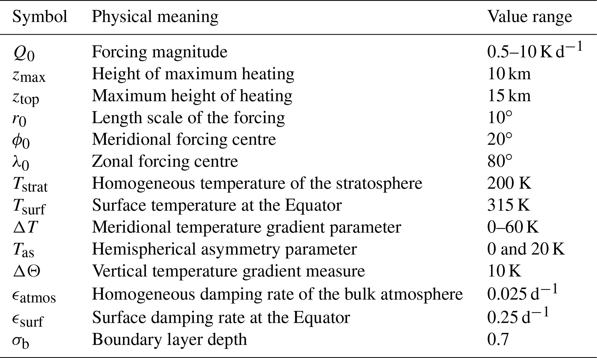
The parameters appearing in Eq. (1) are defined in Table 1. For most of the parameters of the basic state we use the same values as have originally been used by Held and Suarez (1994), with the exception of the meridional temperature gradient parameter ΔT, which we vary to alter the characteristics (in particular the strength) of the induced mid-latitudinal background flow. Following the proposal by Polvani and Kushner (2002), we further added a term “−T_assin ϕ” to the restoration profile in Eq. (1), allowing us to introduce the hemispherical asymmetry associated with the summer season that is of most relevance to the Asian monsoon. The same approach was adapted by McGraw and Barnes (2016) and Chen and Plumb (2014) to investigate eddy transport in the lower atmosphere, both choosing T_as=20 K, a value twice as large as was originally used by Polvani and Kushner (2002). In this study we use both a (hemispherically symmetric) “annual-mean” state (T_as=0 K) and an asymmetric “summer” state (T_as=20 K) in order to assess the significance of differences in the structure of the background state.

Table 1 Physical parameters used in the GCM.

A tropical monsoon flow is forced by imposing a localised steady heating with structure

$$\begin{array}{}\text{(2)}& Q(\mathit{\varphi },\mathit{\lambda },z)=\left\{\begin{array}{l}{Q}_{\mathrm{0}}V\left(z\right){\cos }^{\mathrm{2}}\left(\mathit{\pi }\frac{\mathit{\varphi }-{\mathit{\varphi }}_{\mathrm{0}}}{\mathrm{2}{r}_{\mathrm{0}}}\right){\cos }^{\mathrm{2}}\left(\mathit{\pi }\frac{\mathit{\lambda }-{\mathit{\lambda }}_{\mathrm{0}}}{\mathrm{2}{r}_{\mathrm{0}}}\right)\\ \text{if}|\mathit{\varphi }-{\mathit{\varphi }}_{\mathrm{0}}|<r_{\mathrm{0}}\text{ and }|\mathit{\lambda }-{\mathit{\lambda }}_{\mathrm{0}}|<r_{\mathrm{0}}\\ \mathrm{0}\text{otherwise },\end{array}\right.\end{array}$$

where ϕ and λ represent latitude and longitude, respectively, Q₀ controls the magnitude of the heating, r₀ its horizontal extent and V(z) its vertical structure. The forcing is centred at ${\mathit{\varphi }}_{\mathrm{0}}=\mathrm{20}{}^{\circ }$ latitude and ${\mathit{\lambda }}_{\mathrm{0}}=\mathrm{80}{}^{\circ }$ longitude, with a radius of $r_{\mathrm{0}}=\mathrm{10}{}^{\circ }$. Note that the zonal position of the forcing is completely arbitrary and has no influence on the results, since we did not impose any zonally asymmetric features other than the explicit heating. For easier visualisation of the response we defined the range of longitudes in our domain to be $-\mathrm{120}{}^{\circ }\le \mathit{\lambda }<\mathrm{240}{}^{\circ }$.

The vertical structure V(z) is given by

$$\begin{array}{}\text{(3)}& V\left(z\right)=\left\{\begin{array}{ll}\sin \left(\frac{\mathit{\pi }}{\mathrm{2}}\frac{z}{z_{\max }}\right)& \text{if }z<z_{\max }\\ {\sin }^{\mathrm{2}}\left(\frac{\mathit{\pi }}{\mathrm{2}}\frac{z_{\mathrm{top}}-z}{z_{\mathrm{top}}-z_{\max }}\right)& \text{if }{z}_{\max }\le z<z_{\mathrm{top}}\\ \mathrm{0}& \text{otherwise}.\end{array}\right.,\end{array}$$

The heating is confined to a height below z_top and maximises at z_max. We chose different a structure of V(z) above and below the maximum at z_max in order to reduce the vertical gradient of the heating at lower levels, which weakens the corresponding PV forcing, and therefore de-emphasise the cyclonic lower level part of the forced monsoon response. However, the results presented in this study do not rely on the precise structure of the forcing.

In each simulation the initial state is that of an isothermal resting atmosphere, and the flow is allowed to evolve in the absence of localised forcing (Q₀=0) until it reaches what is effectively a statistically steady state. At least 1000 d was allowed for this. The imposed localised forcing (Eq. 2) with Q₀≠0 is then switched on smoothly over 25 d and subsequently kept steady. Temporal mean states are obtained by averaging the corresponding field for at least 3000 d starting 1000 d after the switch on of the localised forcing. Anomalies are computed as differences between model runs with and without imposed heating. To prevent the build-up of energy at small scales the model includes a parameterisation of sub-grid-scale processes in the form of an eighth-order hyper-diffusion acting on temperature, vorticity, and divergence and damping the smallest represented spatial scales on a timescale of 0.1 d.

Table 1 gives an overview of the parameter ranges for the imposed heating and the basic state used in our experiments.

We checked that all results shown are not sensitive to changes in the hyper-diffusion timescale and the length of spin-up or averaging periods. Further, the response of the model in the upper troposphere and lower stratosphere region was not sensitive to small changes in the details of the bottom drag layer.

2.2 Re-analysis data

Part of our analysis is based on the ERA-Interim (ERA-I) re-analysis dataset (Dee et al., 2011) of the European Centre for Medium-Range Weather Forecasts (ECMWF). The data used in this study are a standard product of the re-analysis dataset and are given on a horizontal 1${}^{\circ }\times$1^∘ grid following the 370 K isentropic surface. Seasonal means are calculated from monthly averaged fields for the years 2000–2009, while snapshots show fields at 12:00 UTC.

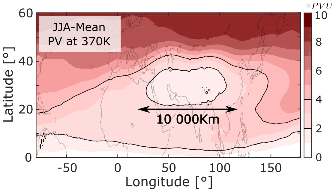
Figure 1 Years 2000–2009 JJA average of ERA-I potential vorticity on the 370 K isentropic surface. The 2 and 4 PVU contours are emphasised, and a length of 10 000 km at 20^∘ latitude is indicated.

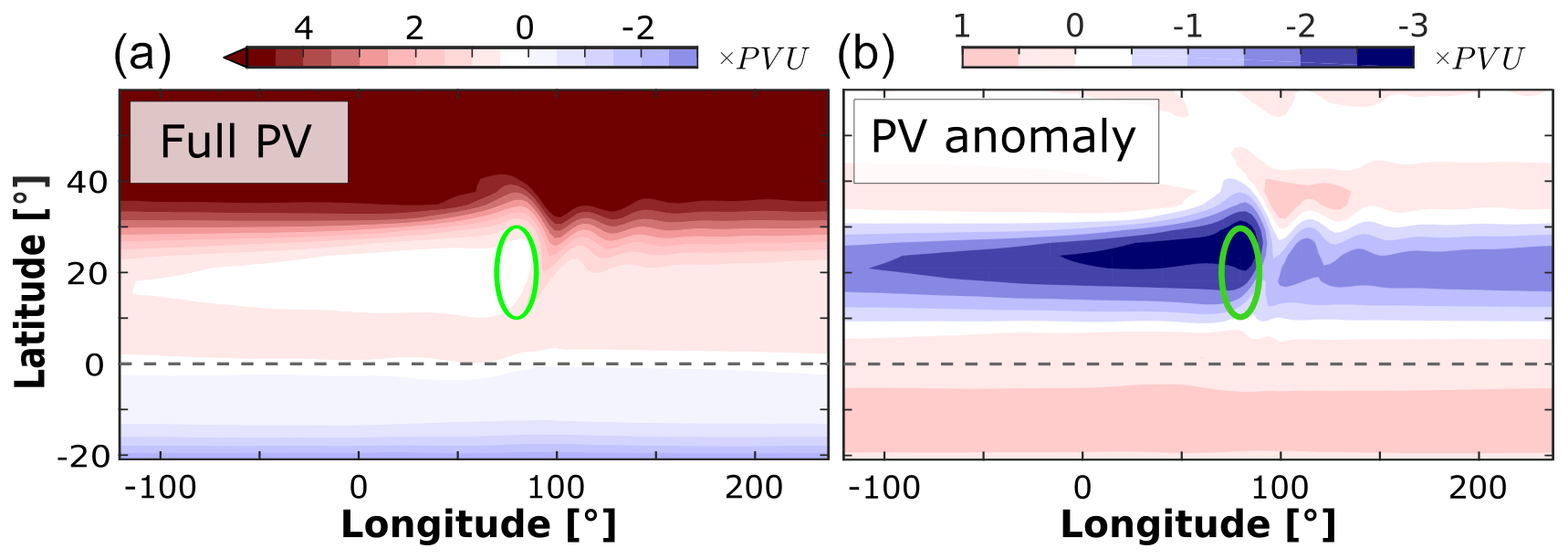
Figure 2 Time-averaged full PV response (a) and PV anomaly (b) on 340 K for a resting basic state with ΔT, T_as=0 to a forcing with Q₀=5 K d⁻¹. Ellipses indicate the horizontal extent of the heating.

3 Zonal scale of the time-mean response

3.1 Localisation due to mid-latitude dynamics

As mentioned earlier the monsoon anticyclone is associated with a pronounced PV minimum in the UTLS region. Figure 1 shows the horizontal structure of this minimum on the 370 K isentropic surface, as it appears in the mean over several NH summers (JJA for 2000–2009). Note that only a limited range of longitudes is included in the figure.

The region of low PV (≤2 PVU) has meridional and zonal widths of about 2000 and 10 000 km, respectively. As explained in Sect. 1 it remains an open question as to what physical or dynamical processes control the zonal localisation of the anticyclone. In this section we conduct a series of numerical experiments to study this problem. In particular we investigate the changes in the response to monsoon heating when varying the meridional temperature gradient parameter ΔT and the asymmetry parameter T_as (see Eq. 1) and thus change the properties of the basic state, including the strength, position and structure of the background mid-latitude jet and the corresponding baroclinic eddies.

We use the numerical model configuration described in Sect. 2.1. Figure 2 shows the time-mean PV structure and the corresponding anomaly from the basic state on the 340 K isentropic surface for a forcing with magnitude Q₀=5 K d⁻¹ and a resting background atmosphere, i.e. ΔT=0 and T_as=0. The chosen isentropic level roughly corresponds to z=13 km at the latitudes of the heating and hence lies between the height of maximum heating (z_max=10 km) and the top of the heating (z_top=15 km) and in a region with strong negative PV forcing due to the large negative vertical gradient of the imposed heating profile. We can therefore expect to observe a relatively strong anticyclonic PV response on this level. From Fig. 2 it is apparent that the PV response is zonally elongated and not confined to the vicinity of the heating. Zonally elongated structures are visible in both the full PV field and the anomaly field (recall that the zonal position of our forcing is arbitrary due to the zonally symmetric basic state, but for ease of comparison we have centred the forcing at 80^∘ N).

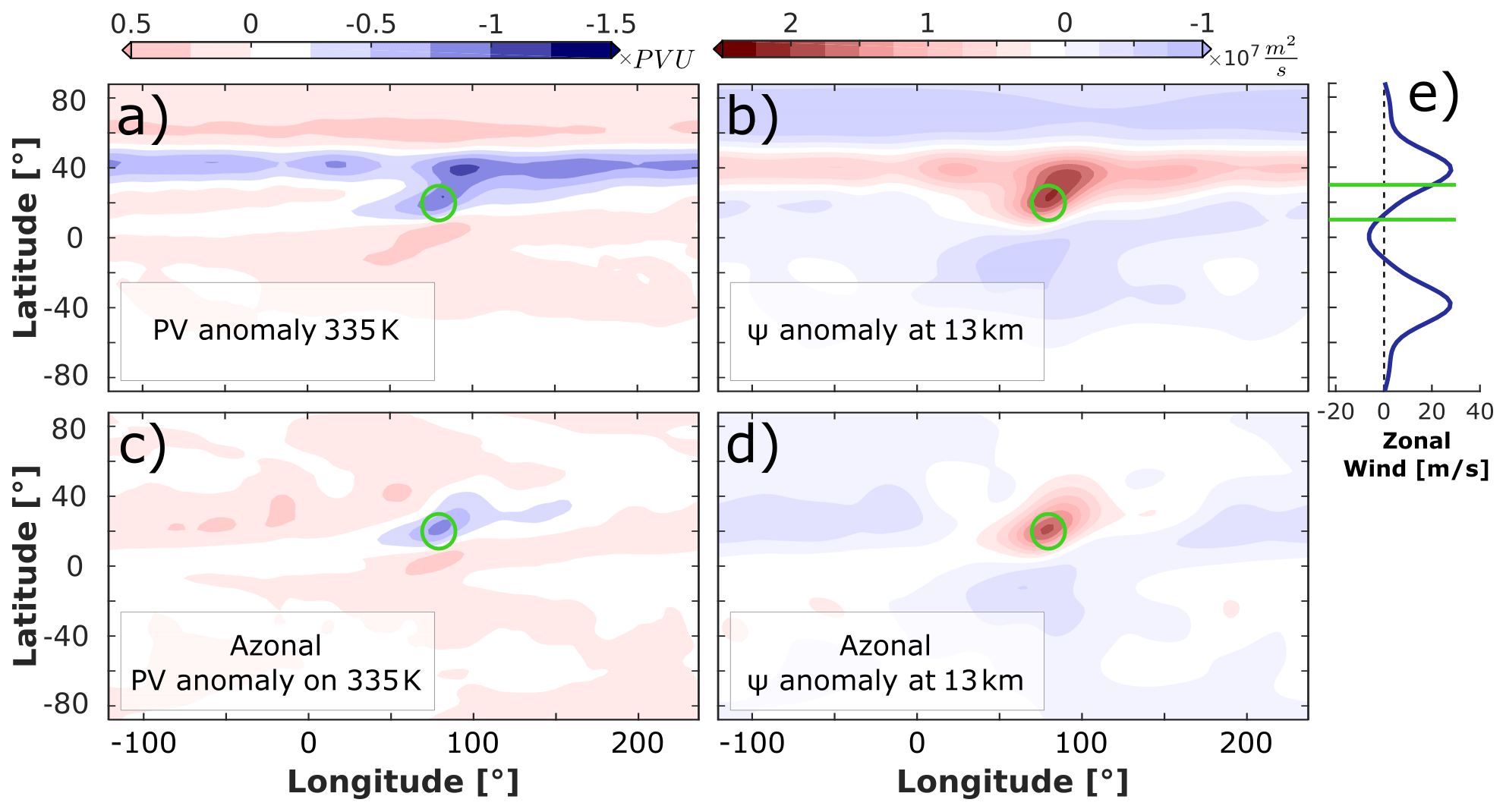
Figure 3 Time-mean potential vorticity anomaly on the 335 K isentrope (a, c) and stream function anomaly on the 13 km surface (b, d) for an experiment with baroclinically unstable background, i.e. the symmetric HS state with ΔT=60 K. The forcing magnitude is Q₀=5 K d⁻¹. The bottom row shows plots with zonal mean removed (azonal anomaly). Circles indicate position and extent of the forcing region. Panel (e) shows the zonal mean zonal wind of the background state at 13 km, with horizontal lines indicating the extent of the forcing region.

Unlike the Gill–Matsuno model (see Sect. 1), our model does not include any mechanical friction above the boundary layer. As a result, the forced Rossby-wave response in the upper troposphere decays only slowly with distance to the west of the forcing, with the controlling process being the weak thermal damping in the bulk atmosphere (timescale of about 40 d)¹. This zonal non-localisation of the monsoon anticyclone is in strong contrast to what is found in re-analysis data (e.g. Fig. 1) and indicates that additional physical or dynamical processes have to be included in the model in order to obtain a monsoon anticyclone response with a realistic zonal scale.

As a next step we modify the basic state of our system by choosing ΔT=60 K in Eq. (1) and thus making the basic state baroclinically unstable at mid-latitudes (for now we keep T_as=0). The resulting dynamics leads to the formation of mid-latitude jet streams with associated highly variable baroclinic eddies.

Figure 3 shows the horizontal structure of the time-mean PV and stream function (ψ) response on the 335 K isentropic surface and the 13 km height plane, respectively². The streamfunction ψ represents the non-divergent part of the horizontal flow. Since we are considering relatively long timescales on which the flow is close to geostrophic balance, the streamfunction is expected to be a useful representation of the actual horizontal flow, which will be non-divergent to a good approximation.

The top panel of Fig. 3 shows the full anomaly response to a localised steady heating in a baroclinically unstable atmosphere. Two main features can be seen:

• a zonally confined patch around the forcing region (green circle) and

• an elongated zonal band of anomaly to the north of the forcing.

The bottom panel of Fig. 3 only shows the zonally asymmetric (azonal) component of the ψ and PV response, i.e. with zonal mean subtracted. We find that the anticyclone response in the form of a confined anomaly patch remains mostly unchanged as we remove the zonal mean, while the northern, elongated feature disappears almost entirely. These results suggest that the change to the background circulation as associated with non-zero ΔT has resulted in a subtropical monsoon anticyclone that is much more zonally confined and that was found with ΔT=0, but the role of the zonally elongated response at mid-latitudes cannot immediately be dismissed, and we therefore examine this further in the following subsection.

3.2 Distinction between response to zonal mean and zonally varying part of the forcing

To further study the nature and relative importance of the zonal band structure seen in Fig. 4 we conduct an experiment using an imposed forcing identical to the one described Sect. 2 but without a zonal mean component (the zonal mean of the original heating was subtracted along the entire latitude band). Figure 4c shows the response of the system to the forcing without zonal mean component. As can be seen, the zonally symmetric band structure is not present in this case, and the PV anomaly response looks almost identical to the response in the case with full heating (including zonal mean), when subtracting the zonal mean of the final response (Fig. 4b). This indicates that the responses to the zonal mean part and to the azonal part of the heating are almost independent, and the zonally extended feature is not caused by the “local contribution” of the forcing but only by its zonal mean component.

In particular the localisation to the west of the forcing is similar in Fig. 4b and c, despite the corresponding basic states differing slightly in their zonal wind structure (due to the changes in wind corresponding to the zonal band structure, also seen later in Fig. 5). This suggests that the direct advection by the mean flow is less important in localising the response and thus that the stirring effect of the baroclinic eddies (which is the other physical ingredient included as a result of non-zero ΔT) potentially plays a significant role. Note that Fig. 4b and c also show indication of an (north-)eastward extension of the time-mean response of the forced anticyclone. We will come back to this feature in Sect. 4 and link it to the phenomenon of eastward eddy shedding.

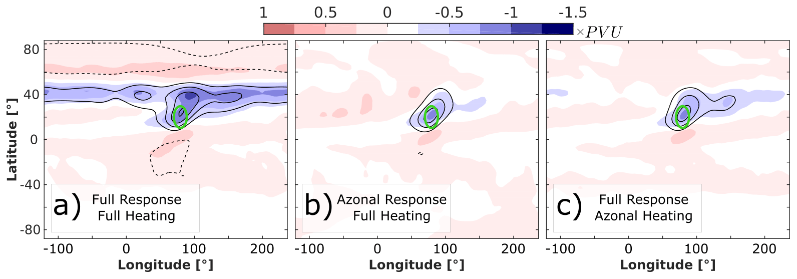
Figure 4 Mean PV anomaly at 335 K (shading) and mean ψ anomaly at 13 km (contours) for the symmetric HS basic state with ΔT=60 K. The contour interval is 5 km²/s. Panel (a) shows the full anomaly response to the full heating. Panels (b) and (c) show the azonal response to the full heating and full anomaly response to a heating without zonal mean, respectively.

The fact that the zonally extended band structure is caused by the zonal mean component of the heating suggests it to represent an annular-mode-like response of the system. Annular modes are hemispheric-scale patterns of climate variability and, in terms of empirical orthogonal functions (EOFs), the leading mode of mid-latitudinal variability (see e.g. Thompson and Wallace, 2000, for a detailed description on annular modes and examples for the observed variability of the atmosphere). A perturbation of the global temperature structure and flow fields by an imposed forcing can cause a response similar to such an annular mode. Effectively, the structure and/or position of the resulting baroclinic jet and eddy features can change as a result of a perturbation. This might lead to a meridional shift of the time-mean jet and can thus manifest as a zonally symmetric PV or ψ structure.

Various studies (e.g. Ring and Plumb, 2007; Butler et al., 2010) have shown that simple dry GCMs with basic states similar to the HS configuration can indeed exhibit an annular-mode-like response when perturbed by a zonally symmetric forcing. As we have shown in Fig. 4, the response to the zonally symmetric part of the heating is manifested in the zonally symmetric part of the response, which can be separated from the zonally localised monsoon anticyclone response forced by the azonal part of the heating.

A characteristic of annular-mode-like responses, in contrast to a simple advection of low (monsoon) PV by the mean flow, is that the coupled system of mean winds and the baroclinic eddies responds as a whole. Figure 5a shows the time and zonal mean zonal wind profile of the HS basic state (contours) and the mean eddy momentum transport, given by the temporally averaged meridional eddy advection of zonal wind $\stackrel{\mathrm{‾}}{u^{\prime }{v}^{\prime }}$ (shading), where u^′ and v^′ describe the deviation of zonal and meridional wind from the zonal mean, respectively, and the overbar indicates the zonal mean. The mean eddy momentum transport is a measure for the strength of the baroclinic eddies and indicates their role in driving the mean flow of the system. Figure 5b shows the corresponding modification of the zonal wind and eddy flux when the system is forced by a local heating with Q₀=5 K d⁻¹. A polewards shift of the jet can be seen, driven by changes in $\stackrel{\mathrm{‾}}{u^{\prime }{v}^{\prime }}$. Note that the mean flow and the eddies seem to respond as a coupled system, and the response is consistent with the typical EOF response associated with annular modes (e.g. Butler et al., 2010).

The results presented above suggest that the elongated mid-latitude feature shown in Fig. 3 has no particular significance with regard to the monsoon anticyclone itself and hence that the addition of the meridional temperature gradient and the resulting baroclinic instability and jet formation is the key ingredient which results in zonal localisation of the monsoon anticyclone response to the confined heating. One has to be careful when interpreting Fig. 5 since the shown anomalies include the localised anticyclone structure in the forcing region that can be seen in Fig. 5b. However, since the change in mean zonal wind is centred at about 40^∘ latitude, and hence north of the forcing, it seems to indeed mostly capture the annular-mode-like feature.

3.3 Sensitivity of the response to details of the meridional temperature gradient

We now investigate in more detail how the monsoon anticyclone response to a confined steady heating changes as we gradually vary the meridional temperature gradient parameter ΔT. This will lead to a change in zonal jet strength, centre position and shape, as well as corresponding changes in the baroclinic eddies. Figure 6 shows the meridional profiles of the mean zonal wind at 13 km. It can be seen how the jets generally shift polewards and become stronger as ΔT is increased. Note that the zonal wind and meridional shear within the forcing region ($\mathrm{10}-\mathrm{30}{}^{\circ }$ latitude) are almost the same for all shown values of ΔT (the exception is the case with T_as=20 K, which we will discuss in a later section).

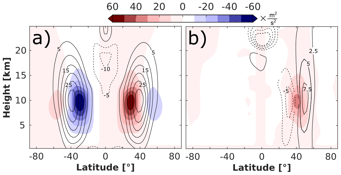
Figure 5 Panel (a) shows time and zonal mean zonal wind field of the symmetric HS basic state (contours) with ΔT=60 K and the time and zonal mean eddy momentum flux $\stackrel{\mathrm{‾}}{u^{\prime }{v}^{\prime }}$ (shading). Panel (b) is as panel (a) but with anomalies from the basic state caused by a forcing with magnitude Q₀=5 K d⁻¹.

Figure 6 Time and zonal mean profiles of zonal wind at 13 km for basic state profiles with different values of the meridional temperature gradient parameter ΔT. The blue dotted line shows the summer state with T_as=20 K; all other profiles show the annual-mean HS state with T_as=0 K. The vertical line indicates the centre of the forcing region at 20^∘ latitude.

Several studies have previously investigated the effect of varying physical parameters in HS-like states, e.g. Zurita-Gotor (2008), who found a similar tendency for poleward shift, strengthening and broadening of the jets when changing the meridional temperature gradient.

The altered background state does affect the time-mean response of the flow to the localised heating, as can be seen in Fig. 7. As we increase the meridional temperature gradient ΔT we see how the distinction between the two features discussed in Sect. 3.2 (localised anticyclone and zonal band structure) becomes more apparent. First, the response gradually becomes zonally localised at the latitudes of the heating, forming a coherent anticyclone in the forcing region. Second, the zonal mean component of the anomaly response seems to shift northward, which can be interpreted as formation of an annular-mode-like response, as shown earlier. Figure 5 shows the jet maximum tends to move polewards as ΔT increases, and a similar polewards shift of the corresponding EOF would not be surprising. Further, the PV anomaly response generally seems to weaken (in particular the zonally symmetric part), and its zonal scale reduces with increasing ΔT (see Fig. 7d), which is potentially explained by the increasing strength of the stirring effect of the active mid-latitude eddy field and further indicates the apparent importance of interactions between the response to the imposed heating and the baroclinic eddies in determining the structure of the flow.

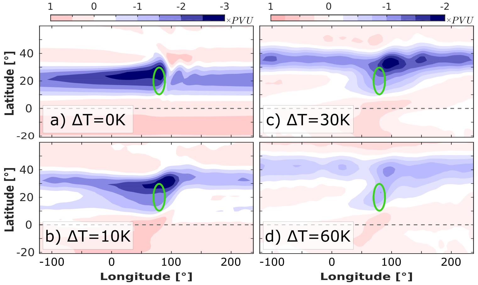
Figure 7 Time-mean PV anomaly response at 340 K (a, b) and 335 K (c, d) for a forcing with magnitude Q₀=5 K d⁻¹ and baroclinic HS basic states with T_as=0 and different values of meridional temperature gradient parameter ΔT. Ellipses indicate the forcing region.

In the rest of this subsection we investigate the response to a steady confined heating for a summer basic state in which hemispheric asymmetry has been incorporated by setting T_as=20 K, as discussed in Sect. 2. The intention is not to contrast the hemispheres but to obtain a basic state that is within the Northern Hemisphere (where the forcing is a located), which is a more realistic representation of the summer state, rather than the more annual-mean-like state of the original HS configuration with T_as=0. Figure 8 illustrates the main difference between the basic state mid-latitude jet profiles for the annual-mean and summer states. Note in particular that the zonal wind for the summer case at a height of 13 km (Fig. 8c) is close to zero in the centre of the forcing region at 20^∘ latitude.

The upper-level ψ and PV response of the summer state to a steady localised forcing are shown in Fig. 9. As for the symmetric case (Fig. 3), we find an annular-mode response, in the form of a zonally symmetric band to the north of the forcing region, and a pronounced localised anticyclone confined to the vicinity of the forcing region. The annular-mode part of the response seems to be broader and span a larger meridional range than that observed in the case with symmetric basic state. The structure of the localised anticyclone, however, seems to be qualitatively similar to the symmetric case. The fact that the localisation of the response in the annual-mean and summer cases is similar while the zonal winds essentially vanish within the forcing region (see Fig. 8) is further evidence that stirring by baroclinic eddies plays a significant role in localising the response, and it is not solely due to the direct advection by the zonal mean flow (also briefly discussed in Sect. 3.2).

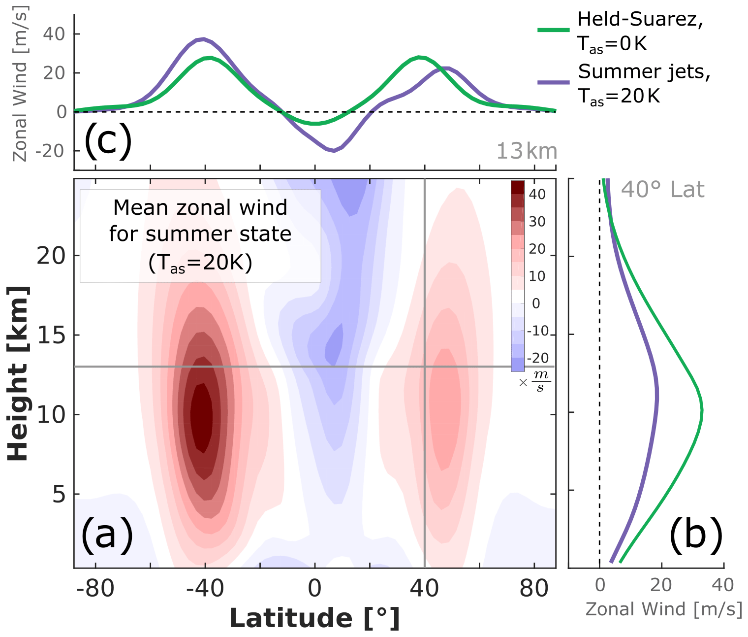
Figure 8 Panel (a) shows the zonal and time-mean zonal wind profile for the summer basic state, using T_as=20 K and ΔT=60 K. Panels (b) and (c) show the zonal jet profiles for the summer and annual-mean cases at 13 km and 40^∘ latitude, respectively, indicated by grey straight lines in panel (a).

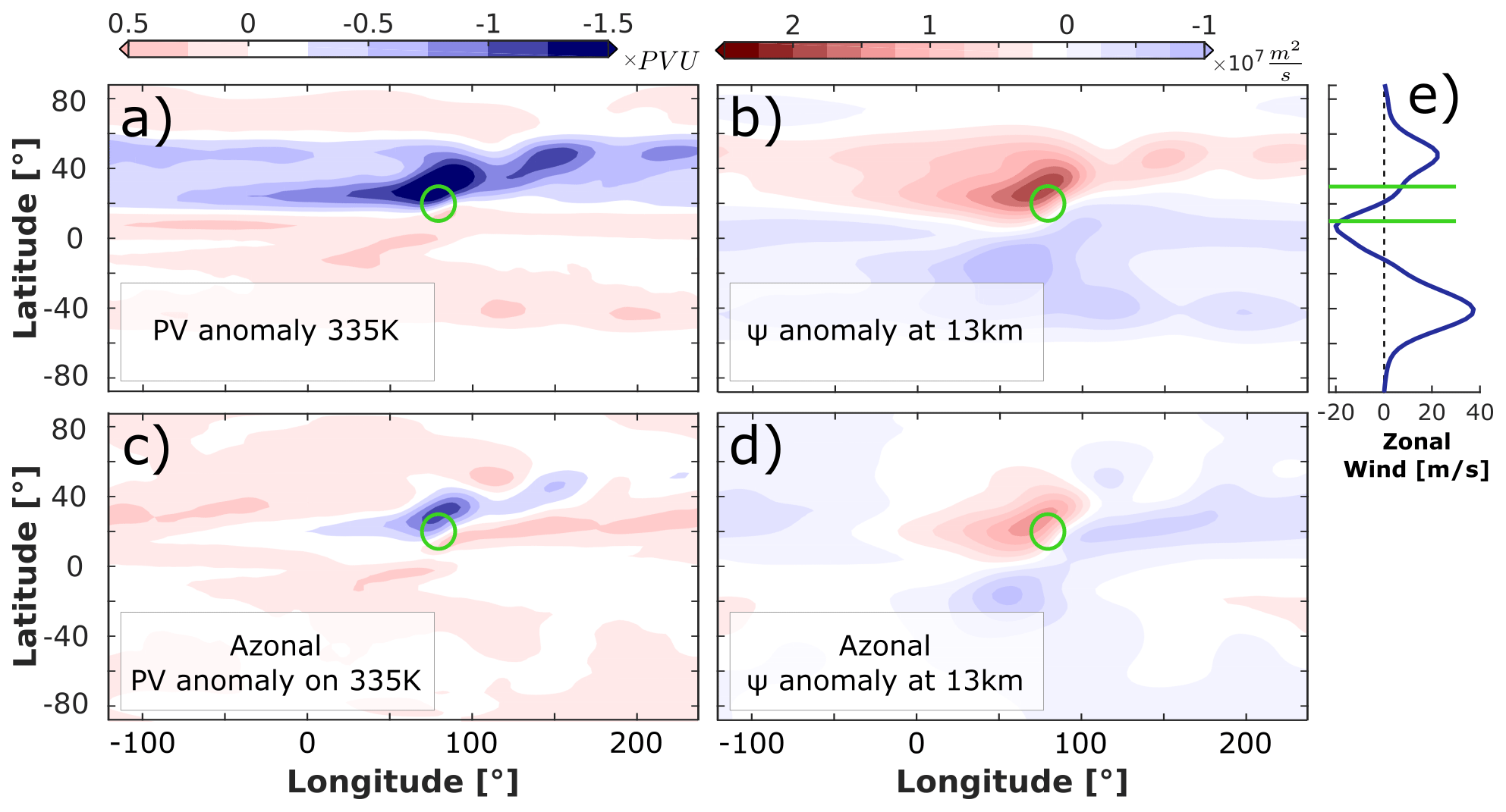
Figure 9 Mean potential vorticity (a, c) and stream function (b, d) anomaly response to a forcing with Q₀=5 K d⁻¹ perturbing the summer basic state with T_as=20 K and ΔT=60 K. Panels (c) and (d) shows the zonally asymmetric part of the response. Circles indicate the forcing region. Panel (e) shows the zonal mean zonal wind of the basic state at 13 km, with horizontal lines indicating the extent of the forcing region.

The azonal mean response seems to show zonal extensions, with the response stretching eastward to the north and westward to the south of the main response, giving the response a north-east/south-west-tilted appearance. Similar extensions can be seen in the symmetric HS case (Fig. 3) although they do not seem to extend as far out of the forcing region and are weaker in magnitude. Further examination (see Sect. 4) suggests that these zonal extensions arise from east- and westward eddy shedding. As we explain, eastward shedding is caused in part by advection by the mid-latitude jet and hence happens preferably closer to the centre of the jet (located north of the forcing), while westward shedding can only occur in the absence of strong eastward winds and hence occurs further to the south (where the zonal winds are weak or even westward). Note that the structure of the monsoon anticyclone PV low in the real atmosphere also shows signs of a north-east/south-west tilt (e.g. the 4 PVU contours around −50 to 50^∘ longitude or the 4 and 5 PVU contours around 150^∘ longitude in Fig. 1), although not as pronounced as for the response in our (highly idealised) numerical simulations.

In the next section we investigate the time dependence of the monsoon response in a baroclinic background, with special interest in the phenomena of east- and westward shedding.

4 Temporal variability in the form of eddy shedding

4.1 Eddy shedding in re-analysis data

As noted in Sect. 1.3, various authors have discussed in detail examples of the evolution of the horizontal monsoon anticyclone PV structure during specific east- or westward-shedding events (e.g. Hsu and Plumb, 2000; Garny and Randel, 2013; Vogel et al., 2014). Figure 10 provides further illustration of shedding events, in this case as observed in re-analysis data during July and August 2000. A localised anticyclone in form of a PV minimum centred at about 30^∘ latitude and 70^∘ longitude can be identified on 11 July in Fig. 10a. Over the following days the northern edge of the anticyclone becomes distorted and the patch of low PV eventually breaks into two almost equally sized anticyclones on 19 July (Fig. 10c). The events between 11 and 19 July are representative for a westward-eddy-shedding event. In the case shown the broken-off anticyclone then slowly propagates westward over the following days. Note that the dynamical evolution of westward-shed vortices (e.g. their propagation speed) can be influenced by interactions with the background flow. Correspondingly the shed vortex discussed above seems to get mostly disintegrated by the meridional wind associated with the baroclinic eddy field over the period until 1 August in Fig. 10f.

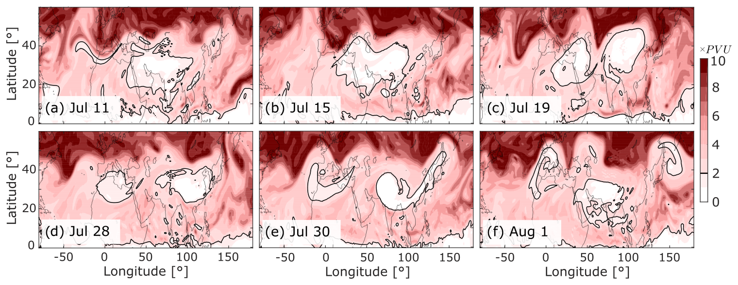
Figure 10 ERA-I potential vorticity on the 370 K isentropic surface for various days of the year 2000. The 2 PVU contour is emphasised. Panels (b) to (d) display the evolution of a westward-shedding event; panels (e) and (f) show an eastward-shedding event.

A few days after the westward-shedding event, on 30 July in Fig. 10e, we can observe an example of an eastward-shedding event. At about 130^∘ longitude one can see how a filament of low PV gets pulled out of the main anticyclone due to meridional advection of a passing-by baroclinic eddy. The filament then breaks off, rolls up and subsequently gets advected eastward by the mid-latitude jet on 1 August (Fig. 10f). Note that, whilst there is significant variation between the daily PV fields (e.g. due to interactions of the bulk monsoon anticyclone with baroclinic eddies) shown in the different panels of Fig. 10, in each case a clear monsoon anticyclone manifested as a coherent low-PV structure (albeit sometimes split into two) can be clearly identified.

4.2 Emergence of westward eddy shedding in model experiments with a basic state at rest

In Sect. 3 we focused solely on the time-mean monsoon anticyclone response of the flow to a steady localised heating. In this Sect. we examine the time variability of this response for a range of forcing and basic state parameters. In particular we show how the phenomena of west- and eastward eddy shedding can spontaneously emerge for certain parameter combinations of the steady forcing and basic state profiles.

As in Sect. 3 we start by considering the case of the forced response in a resting atmosphere, i.e. choosing ΔT=0 in Eq. (1). The corresponding time-mean response was shown in Fig. 2. Figure 11a and b show the instantaneous ψ and PV response to a steady localised heating with two different heating magnitudes, while Fig. 11c and d show the corresponding time evolution of the azonal (with zonal mean subtracted) anomaly response along the 20^∘ latitude line. A clear qualitative difference between both cases with different forcing strength can be seen.

The response to the weak forcing (Q₀=0.5 K d⁻¹) (Fig. 11a and c) is entirely steady and simply consists of a westward-extending beta-plume which slowly decays with distance to the forcing, probably due to the weak thermal damping of the model (as also mentioned in Sect.  3.1). In the case with a strong heating (Q₀=5 K d⁻¹) (Fig. 11b and d) the behaviour of the model is completely different. In this case the system exhibits a periodic creation and westward shedding of vortices (or eddies) from the region of (steady) heating, inducing a strong temporal and zonal variability. Note that these structures represent distinct and coherent eddies, rather than a zonally propagating Rossby wave, to the extent that they correspond to closed contours in the full PV field.

The eddies propagate predominantly westward at an essentially constant speed of about 12 m/s, indicated by the constant slope of the diagonal line in Fig. 11d. Different authors have studied the propagation of isolated vortices in simplified settings (e.g. single-layer beta-plane models) and found them to propagate (at leading order) westward with the phase speed of long Rossby waves (e.g. Davey and Killworth, 1984; Cushman-Roisin et al., 1990), although Davey and Killworth (1989b) found that interactions of neighbouring vortices can modify their propagation speed (for further details see Rupp, 2019). In addition to the formation of eddies at the latitudes of the heating we see positive PV anomalies (and corresponding negative stream function anomalies) in the Southern Hemisphere in Fig. 11b. These structures do not correspond to closed contours in the full PV field and are likely to be essentially a Rossby wave response forced by the eddy shedding and eddy propagation process. The spontaneously emerging temporal variability of the response to a steady forcing that can be seen in Fig. 11 is a potential explanation for the observed phenomenon of westward eddy shedding in relation with the observed monsoon anticyclone (e.g. Fig. 10).

Figure 11 (a, b) Day 1500 snapshot of the stream function anomaly response at 13 km in an atmosphere at rest (ΔT=0, T_as=0) for two different forcing magnitudes. Contour lines show the day 1500 PV anomaly on the 340 K isentropic surface, with dashed contours representing negative values, the zero contour not shown, and the contour interval being 0.2 and 1 PVU for panels (a) and (b), respectively. The ellipses indicate the forcing region. (c, d) Evolution of azonal stream function along line at 13 km and 20^∘ latitude for the same two experiments shown in the top panel. Vertical lines indicate the extent of the forcing region; the slope of the diagonal black line in (d) indicates a reference velocity of 12 m/s.

Note that, as discussed in Sect. 3, the lack of strong dissipation in our model leads to an extreme westward elongation of the response and an eventual re-emergence of air parcels in the forcing region due to the spherical geometry of the domain. In cases where the system is in the shedding regime, i.e. with strong heating magnitudes, this phenomenon can, in particular, lead to a “phase-locking process”, where vortices that re-emerge in the forcing region can trigger a new shedding event. Such a phase-locking mechanism can potentially influence flow characteristics like the shedding frequency or the size of shed vortices, and the corresponding details of the response have to be interpreted with caution. Other authors have previously investigated eddy shedding in a periodic domain but either restricted their experiments to early time behaviour (Davey and Killworth, 1989a) or did not mention the phenomenon of phase locking (Hsu and Plumb, 2000). However, phase locking is less relevant for experiments in which the response is, via some process, zonally localised, for example experiments that include a representation of mid-latitude dynamics (as discussed in Sect. 3).

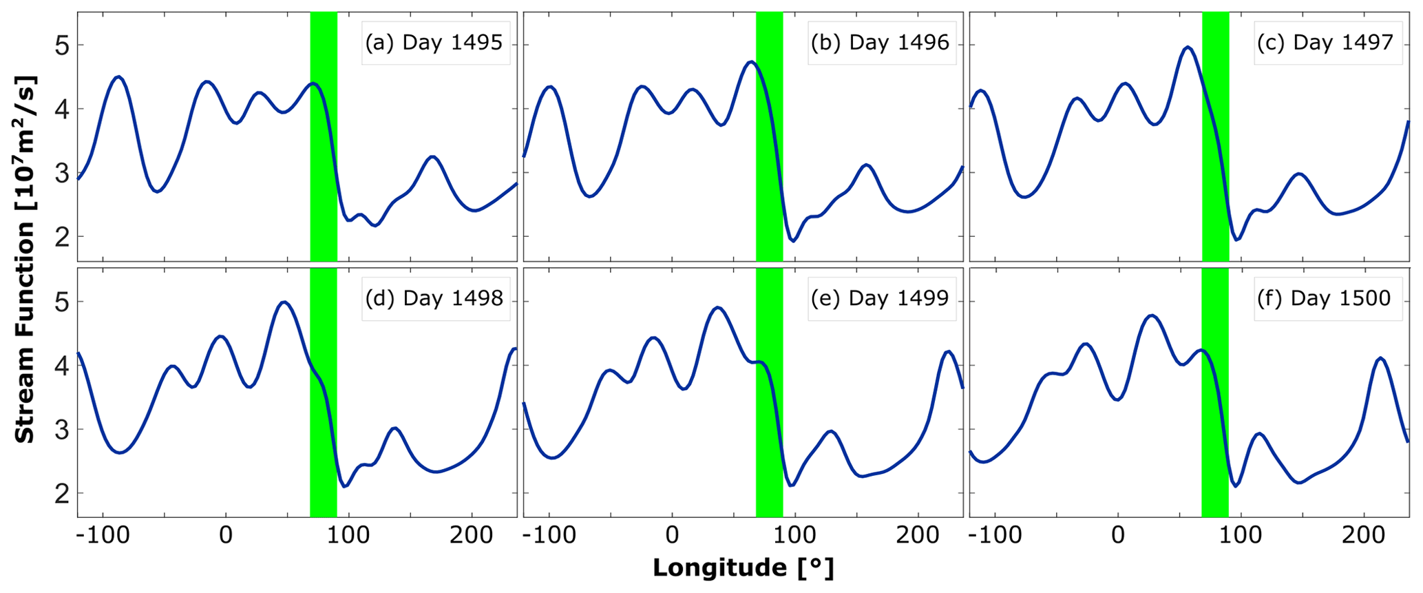
Figure 12 Evolution of the stream function response at 13 km and 20^∘ latitude over several days in an atmosphere at rest (ΔT=0, T_as=0) and for a forcing magnitude of Q₀=5 K d⁻¹. The vertical shading indicates the forcing region.

In order to obtain a better understanding of how the westward-shedding process evolves, Fig. 12 displays the structure of ψ along the 13 km and 20^∘ latitude line for several consecutive days. Zonal profiles through the centre of the forcing region are a suitable way of describing the flow evolution since the meridional structure of the response varies little with longitude and is mostly determined by the meridional structure of the imposed forcing, as can be seen in Fig. 11b. At day 1495 (i.e. Fig. 12a) we find a localised anticyclone developing inside the forcing region (given by a local maximum in ψ) and slowly strengthening and propagating westward over the next few days. As it moves out of and away from the forcing region the stream function inside the forcing region decreases slightly (see Fig. 12d). Once the anticyclone moved sufficiently far away from the forcing, another isolated vortex starts developing inside the forcing region, and correspondingly the stream function starts to increase again (Fig. 12f). Figure 12 suggests the shedding process to be characterised by the periodic production of individual vortices inside the forcing region along with a continuous predominantly westward propagation of the strengthening vortex (consistent with Fig. 11d), resulting in alternating periods of high and low equatorward flow anomalies within the forcing region and therefore variations of the southward advection of high background PV. We find the evolution of the stream function response during a westward-shedding event in our three-dimensional model to be similar to what has been described by other authors in relation to single-layer studies on westward shedding (Hsu and Plumb, 2000; Davey and Killworth, 1989a).

For the rest of this section we focus on experiments in the shedding regime, i.e. experiments with imposed heating of magnitude, and investigate the details of the intrinsically emerging temporal variability for various basic state configurations.

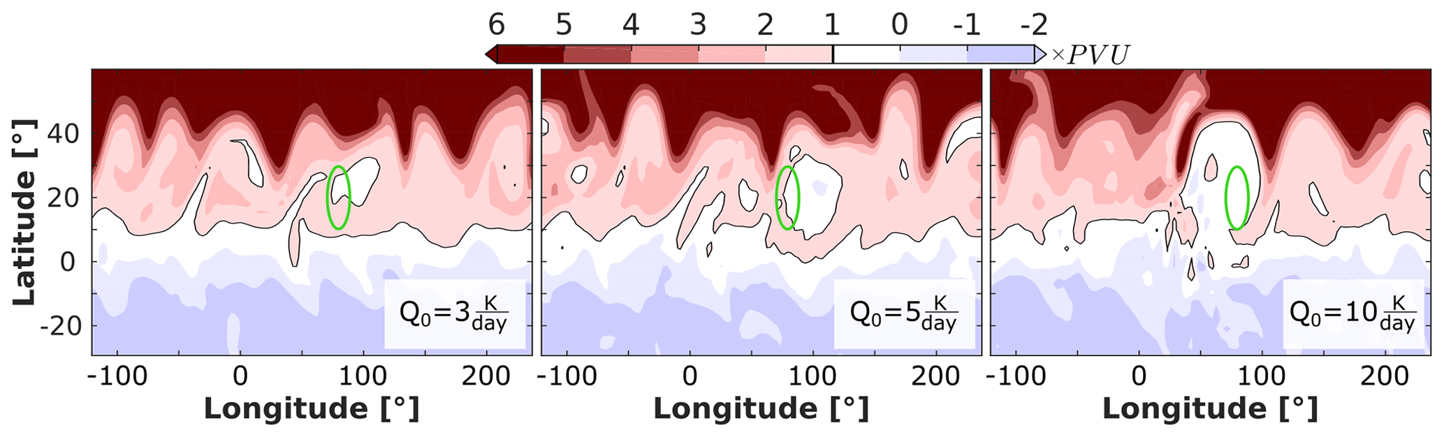
Figure 13 Day 1525 PV response at 335 K using different forcing magnitudes and a symmetric HS state with ΔT=60 K. Ellipses indicate the forcing region, and the 1 PVU contour is highlighted.

4.3 Transition to eastward eddy shedding via introduction of mid-latitude dynamics

Next we investigate how the (transient) behaviour of the response changes as we make the basic state baroclinically unstable by introducing a meridional temperature gradient, i.e. by increasing ΔT in Eq. (2). As mentioned earlier, the baroclinically unstable basic state develops westerly jets and baroclinic eddies in mid-latitudes. The latter induce a strong spatial and temporal variability to the background flow, and hence the PV and stream function fields generally show a range of quickly evolving spatial structures which can correspond to anomalies of fairly large magnitude compared to the time-mean field. Since the response magnitude of the explicitly forced anticyclone strongly depends on the forcing strength (as suggested by Fig. 11) one can imagine situations where the response to a steady localised heating is weak relative to the varying anomalies of the background, and thus it is difficult to identify a clear and pronounced anticyclone on a day-to-day basis. In situations with sufficiently strong forcing, and therefore strong response, one would, on the other hand, expect to see a well-defined anticyclone in terms of a coherent low-PV structure (as is typically the case in re-analysis date; see Fig. 10).

Figure 13 shows instantaneous snapshots of the PV response to heating distributions with varying magnitude Q₀. For the case with Q₀=10 K d⁻¹ a clear patch of low PV can be identified in the vicinity of the forcing region, relating to a clearly visible anticyclone, i.e. similar to the observed cases shown in Fig. 10. For the weaker heating with Q₀=3 K d⁻¹, on the other hand, the anticyclone is barely visible and could easily be misinterpreted for a feature of the basic state (e.g. a baroclinic eddy). This dependence of the response amplitude on the forcing magnitude is a persistent and usual characteristic of the flow. Whilst the PV field of course varies on a day-to-day basis, these overall characteristics of the PV field (as the forcing magnitude varies) are robust and reproducible. In all three experiments shown in Fig. 13 the PV anomaly of the anticyclone becomes clearly visible when taking long time averages since the azonal anomalies of the background state average out and the monsoon response creates a uniquely identifiable azonal feature in or near the heating region.

The nature of time dependence of the response changes fundamentally as we gradually increase ΔT and thus gradually introduce active mid-latitude dynamics. Figure 14 shows the time evolution along latitude lines at the northern edge (top panel) and through the centre (bottom panel) of the forcing region for a range of values of ΔT. In the case where the basic state is at rest (Fig. 14a, b) we find pronounced westward shedding of vortices from the forcing region. The vortices subsequently propagate westward along the 20^∘ latitude line, as described earlier. The shed eddies do not have a strong PV signature at 30^∘. In the case with strong mid-latitude dynamics (Fig. 14g, h), on the other hand, almost no evidence for westward shedding can be seen, but we find clear indication of eastward-propagating coherent features. These eastward shed eddies have pronounced PV signatures at 30^∘, i.e. to the north of the forcing region and closer to the centre of the mid-latitude jet (see Fig. 6), suggesting them to be advected eastward by the background wind.

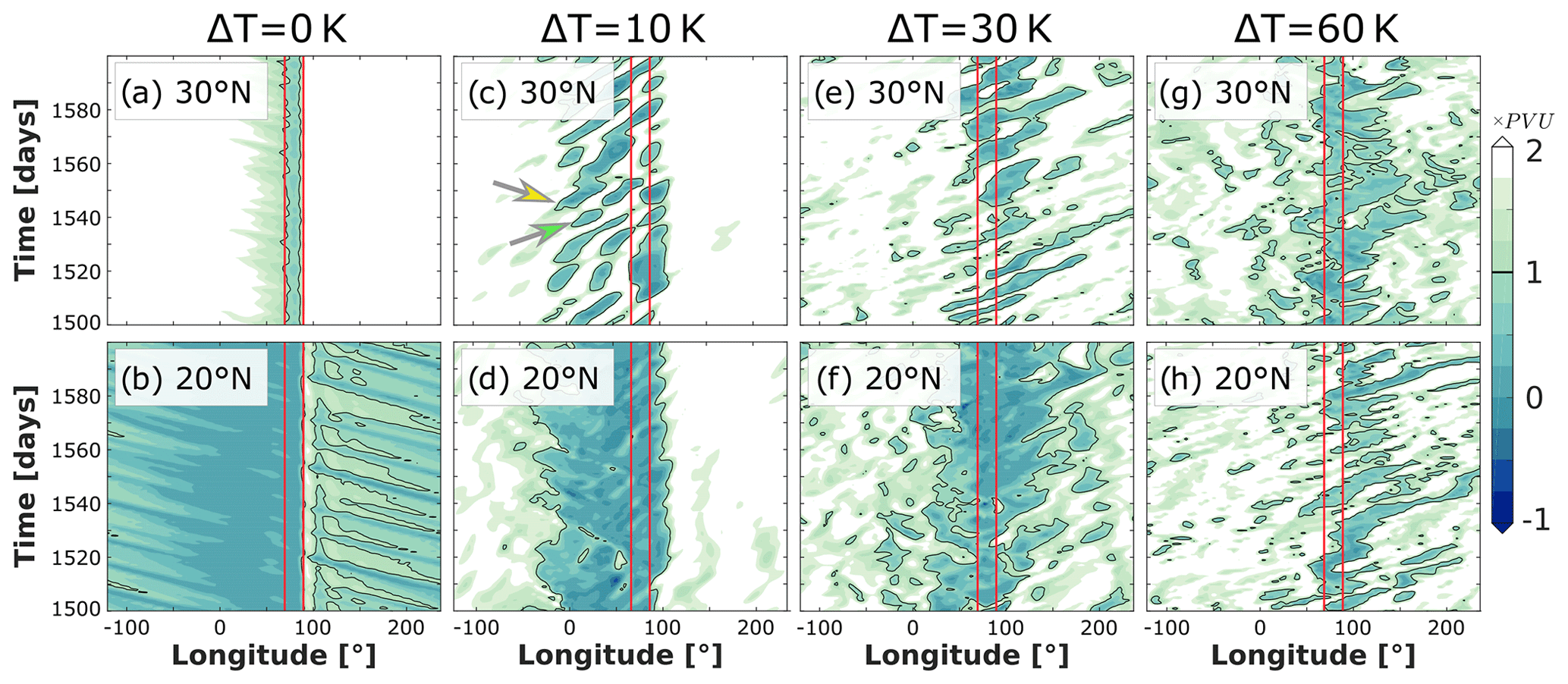
Figure 14 Time evolution of PV along two latitude lines on the 340 K (a–d) and 335 K (e–h) isentropic surface. The forcing magnitude is Q₀=5 K d⁻¹, and the basic state uses T_as=0 and different values of ΔT. Vertical lines indicate the extent of the forcing region, and the 1 PVU contour is highlighted. Arrows show the structures shown in Fig. 16.

To gain a better understanding of the dynamical processes leading to the modified temporal variability of the response in experiments with strong mid-latitude dynamics (e.g. Fig. 14d, h), it is useful to study in detail the evolution of a specific eastward-shedding event. In order to see a clear evolution of the anticyclone on a day-to-day basis (as discussed earlier; see e.g. Fig. 13) we choose a forcing magnitude of Q₀=10 K d⁻¹ for this experiment, although we see similar behaviour for weaker magnitudes (as also suggested by Fig. 14 for Q₀=5 K d⁻¹).

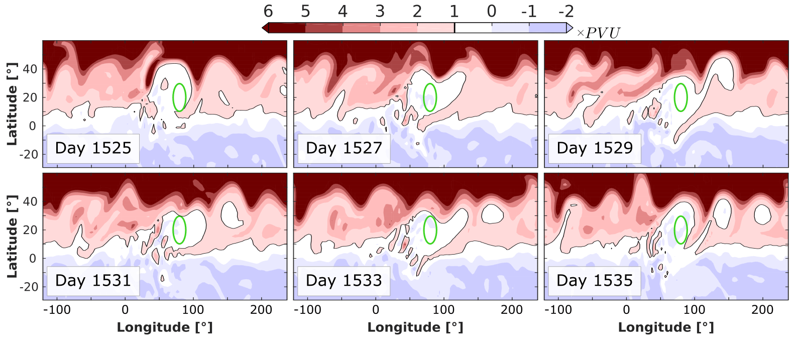
Figure 15 PV response at 335 K for various days. The forcing magnitude is Q₀=10 K d⁻¹, and we used a symmetric HS state with ΔT=60 K. Ellipses indicate the forcing region, and the 1 PVU contour is highlighted.

Figure 15 shows the evolution of PV on the 335 K isentrope over the course of 10 d. Strong wave-like perturbations can be seen along the steep meridional background PV gradient at about 40^∘ latitude, associated with the eastward-moving baroclinic eddies. One can further clearly see a pronounced monsoon anticyclone in the form of a PV minimum in the vicinity of the forcing region (green ellipse), almost elliptic in shape at day 1525. At day 1529 a filament of low PV is pulled out of the bulk-PV region by the strong winds of a baroclinic eddy associated with a sharp PV gradient. The filament then rolls up and breaks off over the following days, forming an isolated anticyclone at day 1531 which subsequently gets advected eastward by the mean zonal wind of the background state. A second such eastward-shedding event is happening between days 1531 and 1535. This behaviour, which in our simulations occurs repeatedly as a response to a combinations of steady monsoon heating and statistically steady baroclinic eddy dynamics in the extratropics, is very similar to what has been reported during specific events (e.g. Enomoto et al., 2003; Garny and Randel, 2013). Note that the centre location of eastward-shed vortices in Fig. 15 is located northward of the forcing region, in agreement with the PV signals observed in Fig. 14e and g.

A slightly different kind of behaviour seems to be happening for the weakly baroclinic background state with ΔT=10 K. As can be seen in Fig. 14d a coherent bulk anticyclone has formed at 20^∘ latitude and between about −20 and 100^∘ longitude. There is no pronounced time variation or preferred direction of propagation obvious, and the response seems relatively steady. However, to the north of the forcing region (Fig. 14c) patches of anomaly seem to appear to the west of the forcing region, propagate eastward towards it and eventually disappear near the eastern edge of the forcing. In the following paragraphs we discuss this state in more detail, before moving on to a (hemispherically asymmetric) summer basic state.

Figure 16 shows how the PV field on the 340 K isentropic surface evolves between days 1542 and 1550 for a background state with ΔT=10 K. The arrows highlight the position of two pronounced baroclinic eddies forming a wave-like structure on the mid-latitude PV gradient of the background. As the eddies move eastward, they start to interact with the PV minimum of the anticyclone. The meridional winds associated with the horizontal gradients in PV pull low PV out of the anticyclone northward on one side and advect high-value PV southward on the other. A potential dynamic interaction of the monsoon anticyclone could then further intensify this baroclinic wave structure. It is also possible that the combination of strong westerlies of the mid-latitude jet and the northern part of the anticyclone forms a sort of wave guide, as pointed out by Enomoto et al. (2003), which additionally favours certain waves and hence leads to a stronger modulation of the PV field.

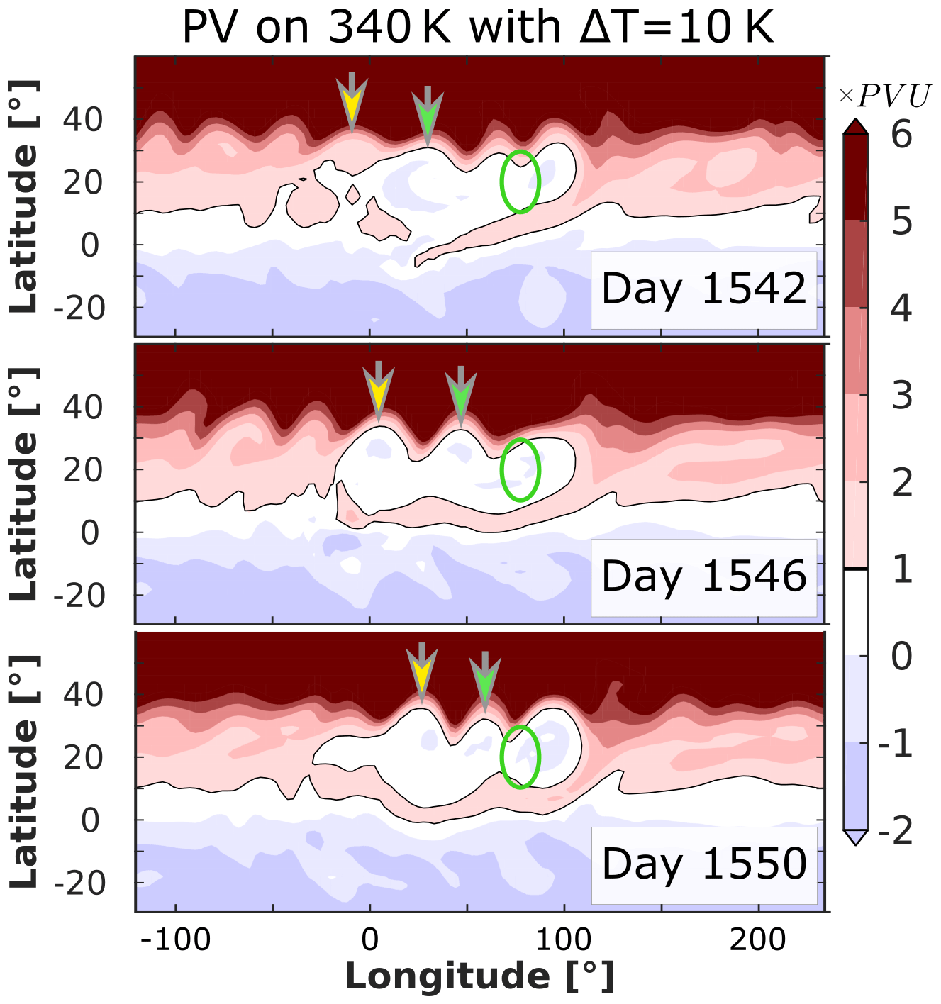
Figure 16 Snapshots of PV at 340 K for a forcing with Q₀=5 K d⁻¹ and a symmetric basic state with ΔT=10 K. Ellipses indicate the forcing region, and the 1 PVU contour is emphasised. The arrows illustrate the position of different wave structures on the sharp PV gradient associated with the jet stream.

Amemiya and Sato (2018) observed a somewhat similar behaviour in a steadily forced single-layer model with meridionally varying mean depth, inducing a background westerly mean wind. They describe a statistically steady localised response, which experiences westward shedding of eddies followed by a circling back of shed vortices towards the forcing region. However, it should also be noted that the basic state used by Amemiya and Sato (2018) is associated with a pronounced reversal of the meridional PV gradient at the latitudes of the imposed forcing due to the varying mean depth of the modelled fluid layer. It is questionable if such a state is a useful representations of the sub-tropical UTLS, as to some extent discussed by e.g. Kraucunas and Hartmann (2007), who argue that sub- and extratropical basic state flows should not be introduced through a layer depth gradient to avoid unrealistic behaviour of the system.

The process shown in Fig. 16 leads to the emergence of coherent PV anomaly structures at about −20^∘ longitude and subsequent eastward propagation of such, as shown in Fig. 14c. However, the meridional advection does not lead to a complete separation of low-PV patches from the bulk anticyclone and subsequent eastward propagation of these patches, as we observe for basic state configuration with stronger meridional temperature gradient (see Fig. 15). A potential explanation is that the baroclinic eddies in the case with ΔT=10 K are too weak to produce sufficient meridional advection of PV and/or are located to close to the forcing region to create elongated PV filaments (recall that the jet core is located farther north for larger values of ΔT).

Different authors have presented indication for the existence of a bimodality of the monsoon anticyclone, with respective east- or westward displacement of the anticyclone centre (e.g. Zhang et al., 2002; Siu and Bowman, 2020). Similar theories suggest the occurrence of a “split state” of the anticyclone, showing two distinct centres (e.g. Vogel et al., 2015). Nützel et al. (2016) found that only one (NCEP-1) out of seven analysed re-analysis datasets showed indication for a pronounced bimodality for a range of timescales. The modulations of the PV low of the anticyclone by baroclinic eddies in Fig. 16 can produce pronounced and zonally separated PV minima on certain latitudes. It is not clear if this mechanism, however, can potentially explain the observation of mentioned split phases in certain diagnostics and datasets.

Since the phenomenon described above modulates the northern edge of the anticyclone, it creates a north–south asymmetry of the PV minimum in the form of a wavy northern edge and an only weakly perturbed southern edge. We find similar modulations of the northern edge in PV fields of re-analysis datasets, e.g. just before a westward-shedding event on 15 July in Fig. 10.

We also observe east- and westward-shedding behaviour in experiments with a (hemispherically asymmetric) summer basic state, i.e. when choosing T_as=20 K in Eq. (1). Figure 17 shows the time evolution of PV along two latitude lines on the 335 K isentrope. Clear evidence for both westward shedding at the latitudes of the forcing region and eastward shedding north of it is visible. Westward shedding seems to occur much more frequently than eastward shedding, and the shed vortices travel much farther. As described for the symmetric cases in Fig. 14 the westward shedding seems to happen mostly on the latitude of the forcing, while eastward shedding has a clear signature to the north of the forcing region. Both characteristics, the north-/southward shift of east-/westward shedding and the relatively more pronounced westward events, seem to be consistent with re-analysis data observations and our general understanding of these features (e.g. Popovic and Plumb, 2001; Enomoto et al., 2003; Vogel et al., 2014).

Figure 17 Time evolution of PV along two latitudes on the 335 K isentrope in a summer basic state with ΔT=60 K. The forcing magnitude is Q₀=5 K d⁻¹. Vertical lines show the extent of the forcing, and the 1 PVU contour is highlighted. Black solid lines indicate an east-/westward velocity of 8 m/s.

A crucial aspect of the relative importance of east-/westward shedding is potentially given by the strength and position of the mid-latitude jet relative to the forcing region. As explained, Fig. 14 shows the change from westward to predominantly eastward shedding as we increase ΔT in the (symmetric) annual-mean HS state. This induces (among other things) a strengthening of the jet and baroclinic eddies; both features are essential for the occurrence of an eastward-shedding process. Hence we find the described transition as the mid-latitude flow becomes stronger with increasing ΔT. In the (asymmetric) summer case we find evidence for both types of shedding, although a clear dominance of westward shedding can be seen. Figure 17 indicates a generally weaker and poleward shifted jet for T_as=20 K, compared to the symmetric case with T_as=0. The existence of such intermediate states, showing signatures of east- and westward shedding, can potentially explain the dominance of the westward-shedding process with respect to eastward shedding in the summer case.

5 Summary and conclusions

In this study we analysed the response of a three-dimensional dry dynamical model to a steady and spatially localised imposed heating distribution, which aimed to model the Asian monsoon anticyclone circulation. Particular focus was given to the modification of the response when the localised forcing was applied to an atmosphere that includes a simple representation of mid-latitude dynamics (mid-latitude jet and baroclinic eddies) compared to an atmosphere at rest. In a range of numerical experiments, we identified a set of characteristics and behaviours that are potentially relevant when describing the three-dimensional circulation of the Asian monsoon anticyclone, including a localised zonal scale and eastward- and westward-eddy-shedding phenomena.

As shown, in re-analysis data the time-mean structure of the PV low associated with the monsoon anticyclone is zonally localised and thus confined to the vicinity of the forcing region. In numerical model simulations with resting basic state (ΔT=0), however, the response to a simple monsoon heating is only very weakly localised, with the anticyclone extending far away from the forcing region and its zonal extent essentially being determined by the weak thermal damping of the upper troposphere and lower stratosphere.

In experiments with mid-latitude dynamics (ΔT≠0) the response forms a localised anticyclone at the latitudes of the forcing and a change in zonal mean flow to north of forcing region. Further examination supports the idea that these two aspects of the response are effectively independent and that the interactions with mid-latitude dynamics allow a time-mean response that is localised to the west and also extends to the (north-)east. We have demonstrated that as ΔT is increased from 0 to 60 K the scale of the anticyclone reduces from several times 10 000 km, which is much larger than the observed scale in the atmosphere, to something less than 5000 km, which is much less than that observed in the real atmosphere. The model is highly idealised, so it would not be appropriate to identify a best value of ΔT, but we conclude that the effect of non-zero ΔT can account for the finite scale of the anticyclone without having to invoke the artificial friction that would be required in the Matsuno–Gill model. Different sensitivities of the response to changes in the background flow suggest the potential importance of the stirring effect of baroclinic eddies in localising the response, in contrast to a mechanism that simply relies on the advection by the time-mean flow. The details of the spatial structure of the anticyclone change as ΔT is varied or the basic state is changed from a more annual-mean state to a state more representative of the summer time conditions in the Northern Hemisphere.

The dependence of some aspects of the spatial structure of the time-mean response on the background is easier to understand if we look in more detail at the time dependence of the system. In the case with resting basic state the response shows a transition from a steady beta-plume state to a state with westward eddy shedding for sufficiently strong forcing. In cases with time-varying basic state the nature of the time dependence of the response changes significantly, and the system exhibits a transition from a state with westward shedding only to a state dominated by eastward shedding as ΔT increases, and thus structure and strength of the background flow change. While in some cases (equinox flow) westward shedding seems to be inhibited, in other cases westward shedding persists (summer flow), and the response shows signs of both shedding behaviours (as observed in the real atmosphere).

The presented model exhibits a range of behaviours and reproduces various properties of the monsoon circulation. The combined simplicity of the setup and ability to simulate different monsoon characteristics provides potential conceptual explanations for many aspects of the monsoon structure and variability and gives a way to study them quantitatively.