the Creative Commons Attribution 4.0 License.
the Creative Commons Attribution 4.0 License.
 | 27 May 2021
The wave geometry of final stratospheric warming events
Daniela I. V. Domeisen
Every spring, the stratospheric polar vortex transitions from its westerly wintertime state to its easterly summertime state due to seasonal changes in incoming solar radiation, an event known as the “final stratospheric warming” (FSW). While FSWs tend to be less abrupt than reversals of the boreal polar vortex in midwinter, known as sudden stratospheric warming (SSW) events, their timing and characteristics can be significantly modulated by atmospheric planetary-scale waves. While SSWs are commonly classified according to their wave geometry, either by how the vortex evolves (whether the vortex displaces off the pole or splits into two vortices) or by the dominant wavenumber of the vortex just prior to the SSW (wave-1 vs. wave-2), little is known about the wave geometry of FSW events. We here show that FSW events for both hemispheres in most cases exhibit a clear wave geometry. Most FSWs can be classified into wave-1 or wave-2 events, but wave-3 also plays a significant role in both hemispheres. The timing and classification of the FSW are sensitive to which pressure level the FSW central date is defined, particularly in the Southern Hemisphere (SH) where trends in the FSW dates associated with ozone depletion and recovery are more evident at 50 than 10 hPa. However, regardless of which FSW definition is selected, we find the wave geometry of the FSW affects total column ozone anomalies in both hemispheres and tropospheric circulation over North America. In the Southern Hemisphere, the timing of the FSW is strongly linked to both total column ozone before the event and the tropospheric circulation after the event.
Please read the corrigendum first before continuing.
-
Notice on corrigendum
The requested paper has a corresponding corrigendum published. Please read the corrigendum first before downloading the article.
-
Article
(8681 KB)
-
The requested paper has a corresponding corrigendum published. Please read the corrigendum first before downloading the article.
- Article
(8681 KB) - Full-text XML
- Corrigendum
- BibTeX
- EndNote


The polar stratosphere exhibits a distinct seasonal cycle featuring a wintertime polar vortex, that is, strong circumpolar westerly winds that form in late summer and decay the following spring, which is ultimately due to the seasonal cycle of incoming solar radiation. While the formation of the polar vortex occurs very predictably each year in late summer of both hemispheres (late August in the Northern Hemisphere and mid-February in the Southern Hemisphere), the timing of the spring weakening of the vortex, the so-called final stratospheric warming (FSW) event, is more variable (Black et al., 2006; Black and McDaniel, 2007a). The FSW marks the reversal of the climatological winter westerlies to summer easterlies in the stratosphere, and its timing varies by up to 2 months in the Northern Hemisphere (NH) and by more than 1 month in the Southern Hemisphere (SH) due to upward-propagating wave disturbances from the troposphere that can disrupt the vortex ahead of its radiatively driven decay (Waugh et al., 1999; Black and McDaniel, 2007a, b). FSWs thus share many characteristics with dynamically driven midwinter disruptions of the polar vortex, spectacular events called sudden stratospheric warmings (SSWs; for a review see Baldwin et al., 2021), in which the polar stratosphere rapidly warms and the polar vortex winds reverse. However, FSW events are driven by a combination of wave-induced and radiative processes (Salby and Callaghan, 2007) and thus occur every spring in both hemispheres, while the occurrence of major SSW events is largely limited to the NH, with a notable exception in the SH spring of 2002 (e.g., Charlton et al., 2005). In the NH, SSWs on average occur about six times per decade (Charlton and Polvani, 2007) with strong decadal variability (Reichler et al., 2012; Domeisen, 2019). Further notable differences between the NH and the SH include a longer lifespan of the SH vortex and a stronger distortion and displacement from the pole of the NH vortex (Waugh and Randel, 1999).
In the SH spring, the timing of the FSW is modulated by feedbacks between chemical stratospheric ozone loss and the circulation (Solomon et al., 2014). The SH spring vortex is climatologically stronger and more stable compared to the NH, resulting in annual conditions ideal for the rapid destruction of ozone by atmospheric chlorofluorocarbons, known as the ozone hole (Solomon, 1999). As sunlight returns to the south pole every year in late September, a cascade of chemical reactions rapidly destroys stratospheric ozone, which further cools and strengthens the polar vortex and allows the vortex to persist longer. The SH thus exhibits a long-term trend in the timing of FSW events that is linked to ozone depletion (e.g., Zhou et al., 2000; Haigh and Roscoe, 2009; Sheshadri et al., 2014). In the NH, where spring temperatures are rarely cold enough to support chemical reactions for rapid ozone loss, the persistence of the vortex in the NH spring is more closely linked to interannual variations in tropospheric wave forcing than to feedbacks with stratospheric ozone (Chipperfield and Jones, 1999; Newman et al., 2001; Savenkova et al., 2012). Nevertheless certain boreal springs, as in 1997 and 2020, have been characterized by a persistent polar vortex associated with extreme Arctic ozone loss (Coy et al., 1997; Lawrence et al., 2020). The timing of the FSW in both hemispheres can have significant influence on the transport and mixing of stratospheric ozone (Rood and Schoeberl, 1983; Manney and Lawrence, 2016). The presence of the polar vortex isolates polar stratospheric air, and so the seasonal breakdown of the vortex allows for the sudden mixing and stirring of vortex air with ozone-rich midlatitude air. The timing of the final warming modulates the strength and speed at which this mixing occurs (Waugh and Rong, 2002).
Just as for midwinter SSWs, changes in the stratosphere at the time of the final warming in spring can have an influence on weather patterns in both hemispheres (Black et al., 2006; Black and McDaniel, 2007a), including extreme events (Domeisen and Butler, 2020). In the SH, the tropospheric eddy-driven jet exhibits an equatorward shift at the time of the FSW related to a negative phase of the Southern Annular Mode (SAM) (Byrne et al., 2017; Byrne and Shepherd, 2018; Lim et al., 2018). The trend and variability in the timing of the FSW event due to ozone depletion has been suggested to further affect the surface impact (Thompson et al., 2011; Son et al., 2013). In the Northern Hemisphere, the FSW is associated with a weakening and equatorward shift of the North Atlantic storm track resembling the negative phase of the North Atlantic Oscillation (NAO), associated with high geopotential height anomalies over the Arctic (Black et al., 2006; Ayarzagüena and Serrano, 2009). Consistent with the chemical-dynamic feedbacks discussed above, spring ozone extremes have also been linked to anomalous surface weather patterns (Calvo et al., 2015; Ivy et al., 2017).
Furthermore, FSW events have been suggested to contribute to variability (Ayarzagüena and Serrano, 2009) and predictability (Byrne et al., 2019; Hardiman et al., 2011; Butler et al., 2019) at the surface. While SSWs cannot be predicted more than 1–2 weeks in advance (Taguchi, 2014, 2016; Karpechko et al., 2018; Karpechko, 2018), FSW events tend to be more predictable, especially events in late spring (Butler et al., 2019). The higher predictability of FSW events with respect to SSW events may provide enhanced lead times for potential surface impacts in comparison to SSW events. For a comprehensive comparison of the predictability timescales of sudden and final stratospheric warming events, see Domeisen et al. (2020).
SSW events have been classified according to a range of characteristics (Butler et al., 2015), notably with respect to the zonal wavenumber dominating the polar stratosphere at the time of or just prior to the event (Bancalá et al., 2012; Barriopedro and Calvo, 2014) or according to vortex elliptical moment diagnostics (Waugh, 1997; Charlton and Polvani, 2007; Mitchell et al., 2011; Seviour et al., 2013), that is, whether the vortex splits into two vortices or displaces off the pole. They have also been classified with respect to their downward impact (Kodera et al., 2016; Runde et al., 2016; Karpechko et al., 2017; Charlton-Perez et al., 2018; Domeisen, 2019; Afargan-Gerstman and Domeisen, 2020). FSW events, on the other hand, have generally been classified according to the timing of their occurrence into “early” and “late” events (e.g., Waugh and Rong, 2002) and their altitude of origin in the stratosphere (Hardiman et al., 2011).
Planetary wave activity from the troposphere to the stratosphere is on average stronger in austral spring compared to austral winter or boreal spring (Randel, 1988; Wang et al., 2019). Climatologically, in the SH late winter and spring the wave structure in the stratosphere is dominated by a quasi-stationary zonal wavenumber 1 (hereafter: wave-1) with contributions from a transient, eastward-moving zonal wavenumber 2 (hereafter: wave-2) (Randel, 1988; Mechoso et al., 1988; Manney et al., 1991; Waugh and Randel, 1999; Harvey et al., 2002; Ialongo et al., 2012), which may contribute to zonal asymmetries in ozone depletion (Kravchenko et al., 2012). In the NH, early FSW events tend to be predominantly wave-driven (e.g., Vargin et al., 2020). In fact, there is no mechanistic difference between midwinter SSW events and early NH FSW events; they are merely differentiated through the evolution of the stratospheric winds after the event as the definition of the SSW requires the winds after the event to return to westerly for a consecutive number of days (Charlton and Polvani, 2007). Late FSWs may also be partly wave-driven, although as the mean flow weakens in boreal spring due to changing solar radiation, less weakening by waves is required for an event to occur. Sun et al. (2011) show in a model study that FSW events tend to occur earlier if wave driving is increased, and a correspondence has been found between the amplitude of wave-1 and the NH FSW date (Savenkova et al., 2012). Wave geometry can also be associated with the nonlinear resonance of the vortex, a process suggested to be potentially important in SH spring (Scott and Haynes, 2002; Plumb, 2010). Given the timing of FSW events in spring when the polar vortex has already weakened, one could hypothesize that these events are more often caused by higher zonal wavenumbers (e.g., waves 2 and 3) as compared to wave-1, as these will be allowed to propagate into the weaker winds (Charney and Drazin, 1961; Matsuno, 1970; Plumb, 1989). Nonetheless, a classification of individual FSW events in the historical record based on geometrical wave structure, and the influence of the wave geometry on stratospheric ozone and surface impacts, does not yet exist.
This study explores the classification of FSW events by wave geometry (Sect. 2), the connections between wave geometry and dynamical behavior in the stratosphere (Sect. 3), ozone distribution (Sect. 4), and surface impacts (Sect. 5).
Currently there exists no consistent metric for defining the central date of FSWs. While most metrics detect the FSW when springtime stratospheric zonal winds fall below a certain threshold, different studies have considered multiple pressure levels (Hardiman et al., 2011), single pressure levels at varying latitudes and thresholds (Black and McDaniel, 2007b; Byrne et al., 2017), or definitions along the location of maximum potential vorticity gradient rather than a zonal mean (Waugh and Rong, 2002). In this study, we compare our results for metrics defined at two different pressure levels, 10 and 50 hPa. In particular, we define FSW dates in these two ways:
-
FSW events are detected as the first date before 30 June (31 January) when the daily mean zonal-mean zonal winds at 60∘ latitude and 10 hPa in the NH (SH) are easterly and do not return to westerly for more than 10 consecutive days (e.g., Butler and Gerber, 2018). An advantage of this definition is that it is consistent with the definition of midwinter SSWs, which is based on the reversal of the westerly winds at 10 hPa and 60∘ latitude (Charlton and Polvani, 2007), and can be used identically in the NH and SH. The 10 hPa level is also optimal for detecting dynamic changes in the polar stratosphere (Butler and Gerber, 2018).
-
FSW events are detected as the first date before 30 June (31 January) when the daily mean zonal-mean zonal winds at 60∘ latitude and 50 hPa in the NH (SH) fall below 5 (10) m s−1 and do not return to westerly for more than 10 consecutive days (similar to Black and McDaniel, 2007b, a). An advantage of this definition is that the spring transition in the lower stratosphere may better reflect both chemistry–climate feedbacks associated with trends in ozone and coupling to the surface.
Tables 1 and 2 list the calculated NH and SH FSW dates, respectively, using daily-mean data from JRA-55 reanalysis (Kobayashi et al., 2015) for the January 1958–December 2019 period and for the definitions based at both 10 and 50 hPa. We do not examine FSWs in the SH prior to 1979 because large-scale dynamical features related to stratosphere–troposphere coupling processes are not reliable due to lack of assimilated observations in the SH prior to satellite measurements (Gerber and Martineau, 2018). We compare these dates based on JRA-55 reanalysis to ERA-interim reanalysis (Dee et al., 2011) for the period in common between them, 1979–2019; in general the dates are almost identical but can vary by 1–2 d.
Table 1Dates and classifications for FSW events in the Northern Hemisphere according to JRA-55 reanalysis. Early (late) events are indicated in bold (cursive), referring to a date before (after) the median date of 12 April at 10 hPa and 15 April at 50 hPa. Dates that fall within ±2 d of the median date are not classified as early or late. U=unclassified (methods did not agree according to the criterion outlined in Sect. 2). Superscripts indicate the ERA-interim classification if it was not in agreement with JRA-55 during the 1979–2019 period.
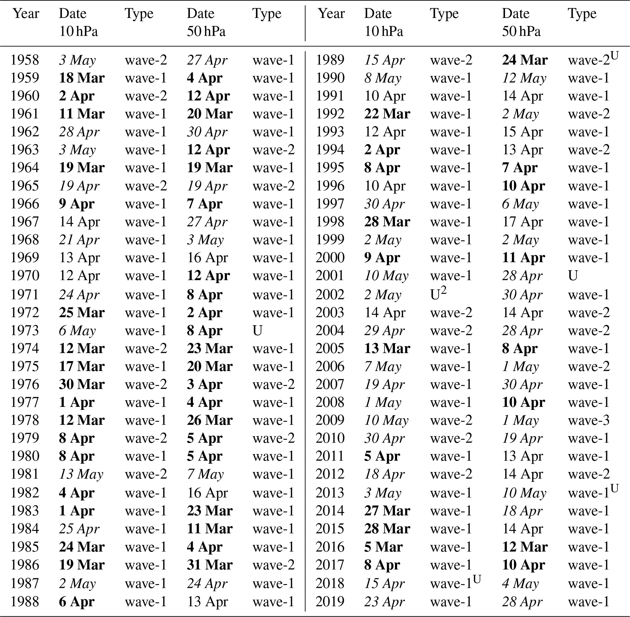
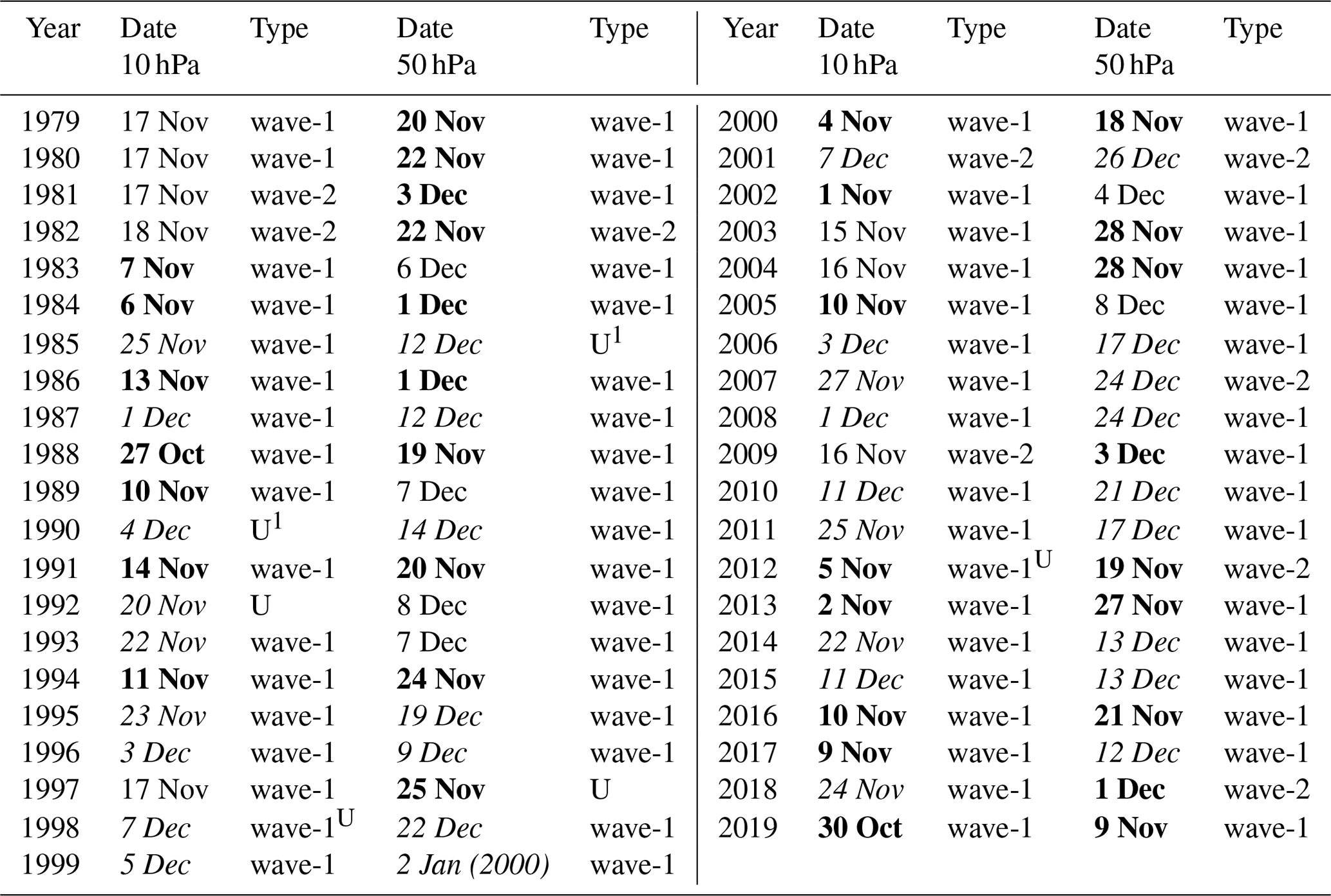
Table 2Dates and classifications for FSW events in the Southern Hemisphere according to JRA-55 reanalysis. Early (late) events are indicated in bold (cursive), referring to a date before (after) the median date of 17 November at 10 hPa and 6 December at 50 hPa. Dates that fall within ±2 d of the median date are not classified as early or late. U=unclassified (methods did not agree according to the criterion outlined in Sect. 2). Superscripts indicate the ERA-interim classification if it was not in agreement with JRA-55 during the 1979–2018 period.
We then classify FSW events by their geometry, either wave-1, wave-2, or wave-3, using the following method. We first apply Fourier decomposition in the zonal direction of the 50 hPa geopotential heights averaged with cosine weighting by latitude over 55–65∘ latitude. The 50 hPa geopotential heights are used for wave classification throughout, no matter the level where the date of the FSW is defined, because wave-2 climatologically peaks at 50 hPa (Barriopedro and Calvo, 2014; Gerber et al., 2021). We determine which wavenumber has, during the period 10 d prior to the FSW date, (1) the daily-mean maximum amplitude for the greatest number of days and (2) the maximum mean amplitude averaged over the 10 d period (similar to Bancalá et al., 2012, and Barriopedro and Calvo, 2014, for midwinter SSWs). The former measures the persistence, and the latter indicates the strength of a given wavenumber; these different metrics frequently but not always yield the same result (see Table A1).
For every event, each of these two metrics indicates a preference for wave-1, wave-2, or wave-3. The final wave geometry classification used throughout the remainder of this study is then determined based on the agreement of these metrics. If they do not agree, the event is labeled as “unclassified”. Table A1 shows the individual classification for each metric for JRA-55, as a demonstration of how the final classification was determined. For the period 1979–August 2019, we check the classifications using both ERA-interim and JRA-55 reanalysis data, as wave geometry for midwinter SSWs has been found to be sensitive to the reanalysis used (Gerber et al., 2021). In general, the classification of FSW events is consistent across the two reanalysis products, although a few discrepancies are noted in Tables 1 and 2.
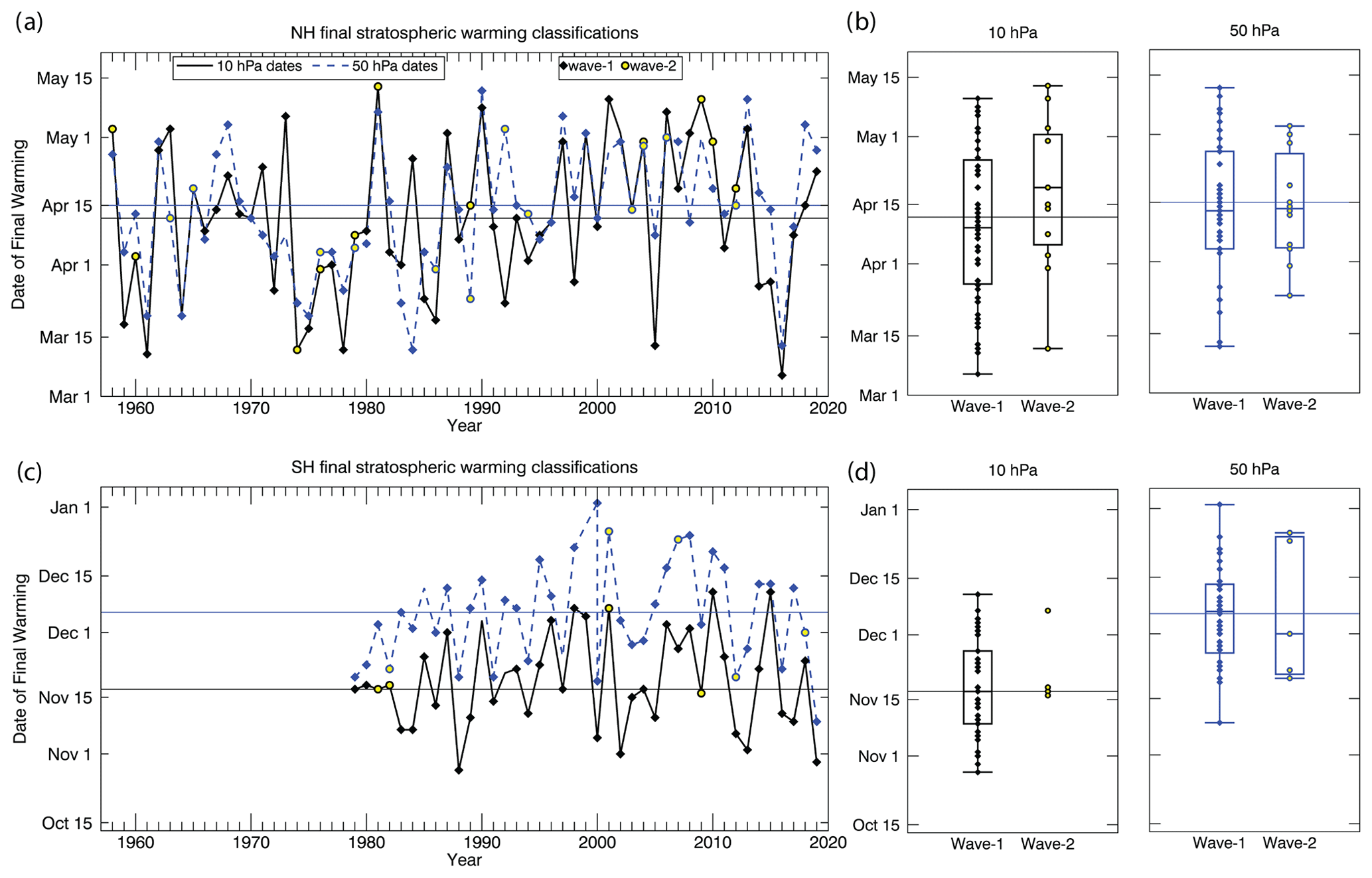
Figure 1(a, c) Dates of FSWs in the NH (1958–2019) and SH (1979–2019) using JRA-55 reanalysis based on zonal-mean zonal winds below 0 m s−1 at 10 hPa (solid black line) and below 5 (10) m s−1 at 50 hPa in the NH (SH) (dashed blue line). Symbols indicate the wave classification of the event. (b, d) Dates of FSWs at 10 and 50 hPa grouped by either wave-1 or wave-2 classification. The whiskers show the earliest/latest dates, the top/bottom of the box shows the upper and lower quartiles, and the solid line shows the median date for each classification. The horizontal lines indicate the median date (based on the 1979–2019 period) for all final warmings in each hemisphere.
Figure 1a and c illustrates the sequence of dates of the final warmings at both 10 and 50 hPa along with their wave geometry classification and their timing of occurrence with respect to the median final warming date, indicated by horizontal lines. In this study we consider separately early events, those that occur more than 2 d prior to the median date, and late events, those that occur more than 2 d after the median date. In the NH, the median date of the final warming based on the 1979–2019 period is 12 April at 10 hPa and 15 April at 50 hPa. In general there is little difference in the timing of the NH FSW for the 10 and 50 hPa metrics, though for a few years they differ by more than a week. In the SH, the median date of the final warming is 17 November at 10 hPa and 6 December at 50 hPa. Given the different classifications for FSW events in the literature, it is important to note that detecting the FSW at 10 or 50 hPa yields a much more significant shift in the timing of the SH as compared to the NH (Newman, 1986). In addition, for the 50 hPa dates in the SH, there is a clear trend towards later FSWs from 1979–2000, and a trend towards earlier FSWs from 2000–2019. While the former has been previously linked to chemical ozone depletion (Waugh et al., 1999), the latter is an indicator of ozone recovery which has recently been tied to a reversal in SH tropospheric circulation trends (Banerjee, Antara et al., 2020). These trends are less apparent for the 10 hPa dates. The linear trend for the 1979–2000 period for the 50 hPa dates is d yr−1, whereas for the 10 hPa dates the trend is d yr−1 (both are significant, but the 10 hPa trend is weaker). Similarly, the linear trend for the 2001–2019 period for the 50 hPa dates is d yr−1, whereas for the 10 hPa dates the trend is not statistically significant at d yr−1.
Nonetheless, the interannual variability in the dates at 10 and 50 hPa is strongly correlated in both hemispheres, at r=0.68 (n=62, ρ<0.01) in the NH and r=0.76 (n=41, ρ<0.01) in the SH. The FSW dates are more variable in the NH compared to the SH; the standard deviations are 18 (15) d for the 10 (50) hPa classification in the NH (1958–2019) and 12 d at both levels for the SH (1979–2019). In the NH, the timing of FSWs has been linked to the occurrence of mid-winter SSWs, which are followed by a period of recovery to westerlies and thus later-than-normal FSWs (Hu et al., 2014). For example for the FSWs at 10 hPa, the median date for years without midwinter SSWs is 1 April, whereas for years with SSWs the FSW date is 24 April. This difference reduces to 4 d for NH FSWs defined at 50 hPa. In the SH, years with larger ozone loss in early austral spring lead via chemistry–climate feedbacks to a colder and more persistent polar vortex and later than average FSWs (Fig. 2; see also Zhang et al., 2017). This interannual relationship holds for both 10 and 50 hPa dates; the correlation coefficient is r=0.53 (n=41, ρ<0.01) between FSW dates at each level and austral spring polar cap total column ozone. Importantly, the median FSW in the NH at 10 (50) hPa occurs only 22 (25) d after the boreal spring equinox, but the median FSW in the SH at 10 (50) hPa occurs 57 (76) d after the austral spring equinox. The much later timing of the SH FSW relative to the seasonal cycle compared to the NH FSW reflects how differing dynamical and chemical processes in the two hemispheres modulate the spring transition; more wave driving leads to earlier FSWs in the NH, while chemistry–climate feedbacks lead to later FSWs (particularly at 50 hPa), compared to if the FSWs were solely driven by incoming solar radiation.

Figure 2Polar cap total column ozone (TCO) (Dobson units) averaged from 7 September–13 October for each year vs. the FSW date in the SH (1979–2019) using zonal-mean zonal winds below 0 m s−1 at 10 hPa (black) or below 10 m s−1 at 50 hPa (blue). The solid (dashed) horizontal line indicates the median date for FSW dates defined at 10 (50) hPa. TCO data are from the Bodeker Scientific filled total column ozone (TCO) database (Version 3.4) (Bodeker et al., 2020); see Sect. 4.
In terms of wave classification, there are fewer wave-2 events compared to wave-1 events, particularly in the SH. In the SH, there are 4 (5) wave-2 events compared to 35 (34) wave-1 events using the 10 (50) hPa dates for 1979–2019. In the NH, there are 13 (12) wave-2 events compared to 48 (47) wave-1 events using the 10 (50) hPa dates for 1958–2019. This frequency of wave-2 events in the NH is slightly larger than the frequency of wave-2 midwinter SSWs (e.g., Barriopedro and Calvo, 2014, who found nine wave-2 events in the 1958–2010 period, using a similar wave classification method). For the NH 10 hPa dates, wave-2 events occur slightly later than wave-1 events (Fig. 1b), with 8 out of 13 wave-2 events from 1958–2019 occurring at least 2 d later than the median date of 12 April. However, for NH 50 hPa dates and for dates at both levels in the SH, no statistical difference between the date of wave-1 and wave-2 FSW events is observed (Fig. 1b and d).
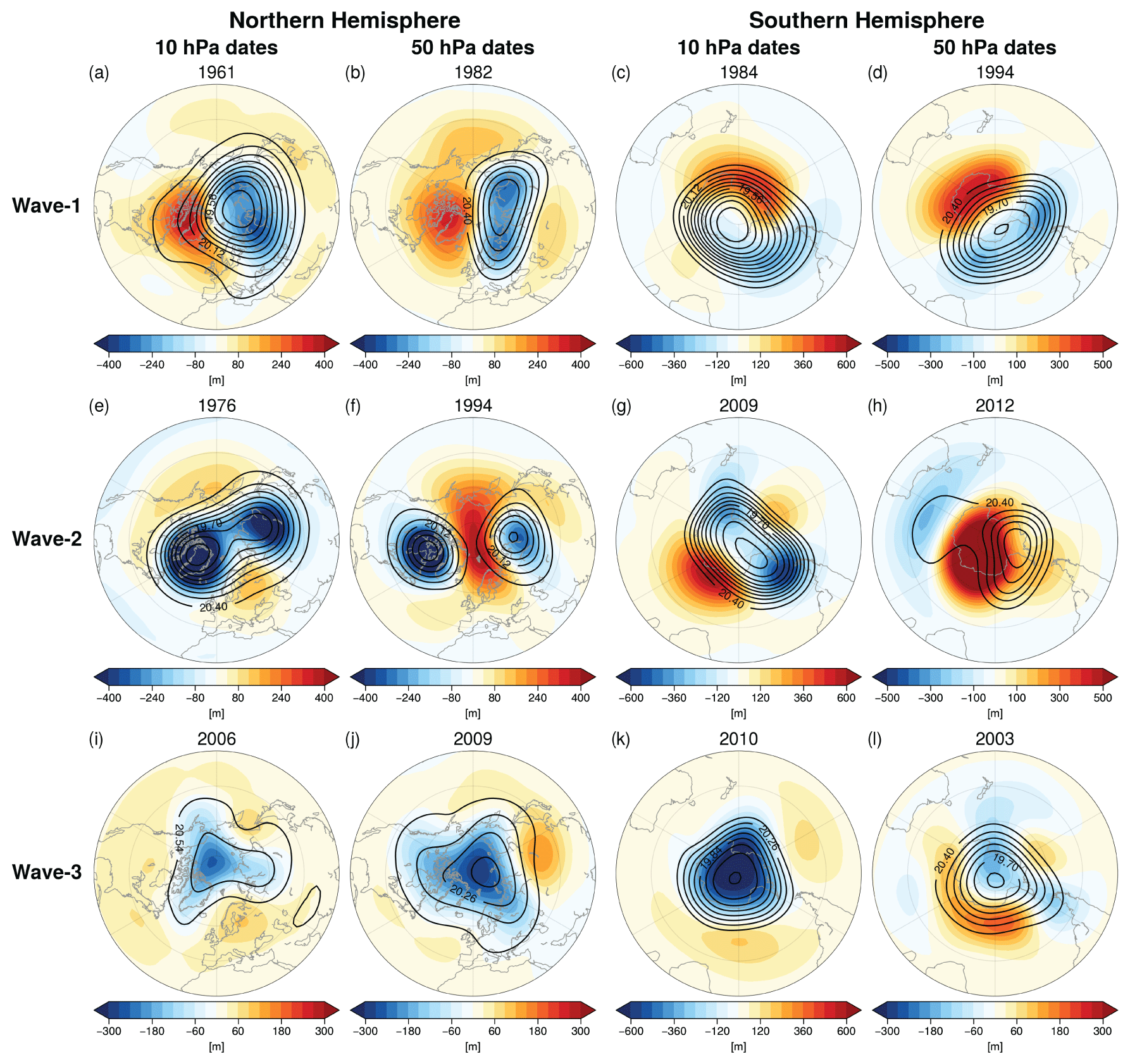
Figure 3The 50 hPa geopotential heights (contours; km) and anomalies (shading; m) from JRA-55 reanalysis averaged over the 10 d prior to the final warming for selected case studies that show a clear wave structure for (a–d) wave-1, (e–h) wave-2, and (i–l) wave-3 for both hemispheres and for FSWs dates at both 10 and 50 hPa. Note the different color bars.
For illustration, Fig. 3a–h show selected wave-1, wave-2, and wave-3 cases of FSWs. Different years were selected in order to showcase the presence of wave structures throughout the record. The wave-1 and wave-2 events show geopotential height structures that are strongly reminiscent of the structures observed during wave-1 and wave-2 midwinter SSW events, with the vortex shifted off the pole during wave-1 events and either elongated or split into two smaller vortices during wave-2 events. Quantification of the wave-3 component using the Fourier decomposition method reveals a substantial role of wave-3 in some cases, highlighted in Fig. 3i–l. There is one NH FSW based on the 50 hPa dates, 1 May 2009 (Fig. 3j), that was classified as a wave-3 event.
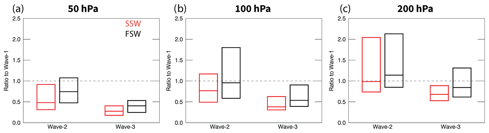
Figure 4Ratio of wave-2 and wave-3 amplitudes relative to wave-1 amplitudes averaged for the 10 d prior to either midwinter SSW events (red) or FSW events (black) for the 1958–2019 period in the NH at (a) 50 hPa, (b) 100 hPa, and (c) 200 hPa. The top/bottom of the boxes show the quartile range and the solid horizontal line shows the median value for 35 midwinter SSW events and 62 FSW events. The dashed line shows where the ratio of amplitudes is equal to 1. The midwinter SSW dates are from Butler et al. (2017).
Evidence that wave-3 plays a more significant role in NH FSW events compared to midwinter SSW events is provided by comparing the ratio of wave-2 and wave-3 amplitudes to wave-1 amplitude averaged for the 10 d prior to SSW and FSW events (Fig. 4). For both SSWs and FSWs, wave-2 and wave-3 amplitudes tend to be more comparable to wave-1 amplitudes in the troposphere (200 hPa), while in the lower stratosphere (50 hPa), wave-2 and wave-3 typically have smaller amplitudes than wave-1 (indicated by median ratios less than 1), as expected from wave filtering (Charney and Drazin, 1961). Wave-3 amplitudes are generally much smaller relative to wave-1 and wave-2 prior to SSWs. This is true for FSWs as well; however, the median ratios of both wave-2 and wave-3 relative to wave-1 for FSWs are higher than for SSWs at all levels (particularly at 50 hPa), suggesting that wave-2 and wave-3 are able to propagate higher as the westerly flow weakens in spring.
In this section we investigate the stratospheric dynamical characteristics of the final warming events. Composites of the 50 hPa geopotential heights and anomalies averaged for the 10 d prior to FSW dates at both 10 and 50 hPa (Fig. 5) shed light on how robust the features in Fig. 3 are across events and for different classifications. First, we focus on the NH (Fig. 5a–h). Wave-1 FSWs defined at both 10 and 50 hPa (a and b) show a shift of the polar vortex towards Eurasia, with corresponding anomalously positive stratospheric height anomalies over North America. Wave-2 FSWs (e and f) instead show an elongated vortex centered over the pole and extending across Canada to eastern Asia, corresponding to anomalously positive stratospheric height anomalies over the North Pacific and Europe. These features do not show substantial differences between the 10 and 50 hPa FSW dates. Comparing early (c and d) and late (g and h) events in the NH indicates that on average early events manifest similarly to wave-1 events, with a shift of the vortex towards Eurasia. The early events for 10 hPa dates have more significant negative anomalies over Eurasia compared to the early events for 50 hPa dates. Late events on average show a more annular response representing (by definition) a stronger vortex compared to average for those dates, though overall the vortex is smaller and weaker compared to early events.
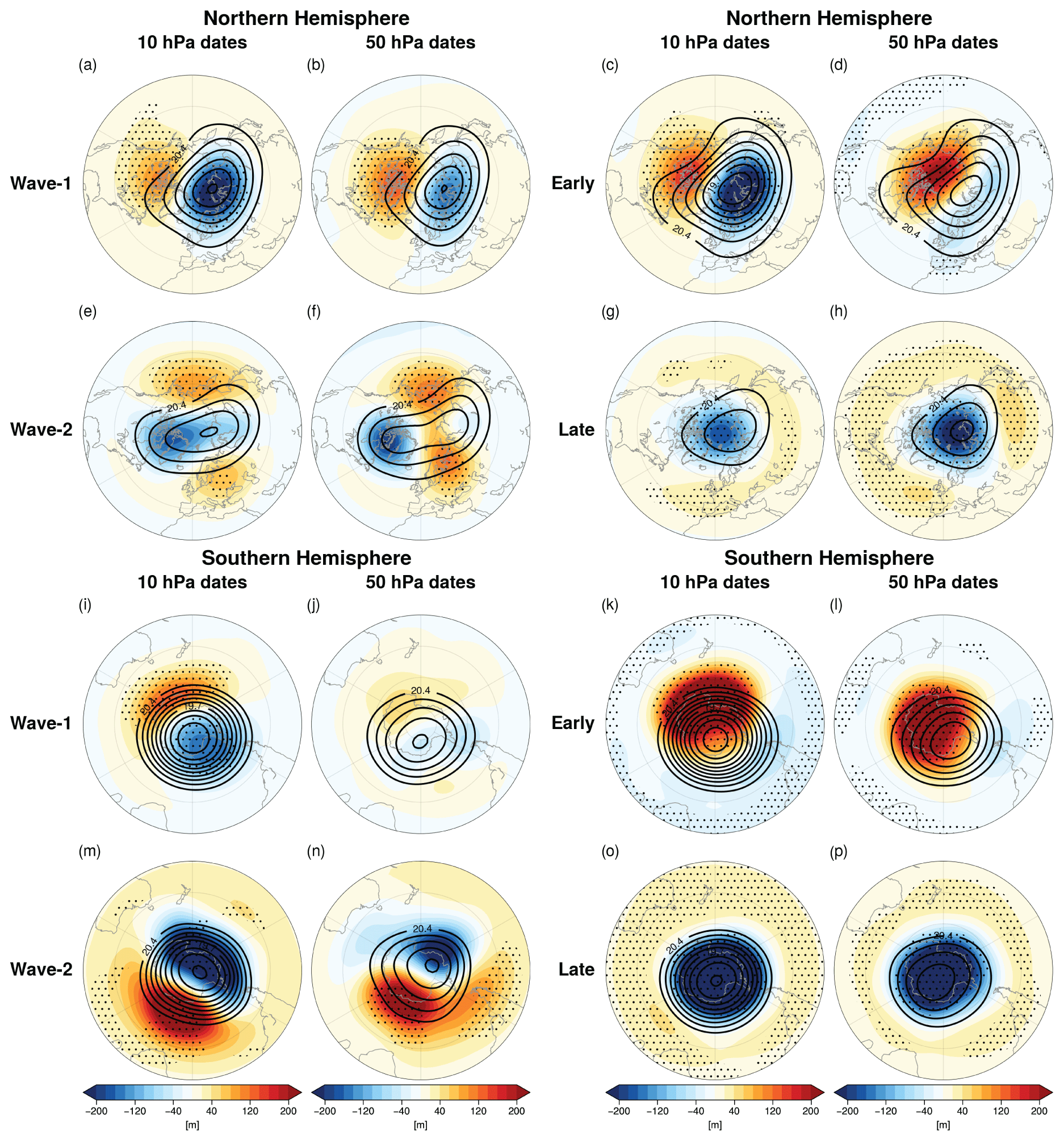
Figure 550 hPa geopotential heights (contours, [km]) and anomalies (shading; m) from JRA-55 reanalysis averaged over the 10 d prior to the final warming at both 10 and 50 hPa for (a–h) the NH and (i–p) the SH. Panels show the composites based on wave-1 or wave-2 classification, or early or late classification. Stippling indicates regions where the anomaly composites are significantly different from zero at the 95 % confidence level according to a two-tailed t test.
In the SH (Fig. 5i–p), wave-1 cases (i and j) on average show a displacement of the vortex towards the Weddell Sea, with anomalously positive height anomalies south of Australia. This wave-1 pattern is only significant for the 10 hPa dates, while wave-1 events for the 50 hPa dates (generally later in austral spring) do not as consistently displace the vortex in a preferred location. Wave-2 events (m and n) for both 10 and 50 hPa dates show negative stratospheric height anomalies over the South Pacific, with anomalously positive height anomalies south of Africa, but overall the wave-2 structure seen in individual cases (Fig. 3g and h) is unclear in the composite (though sample size is small). Robust differences between early (k and l) and late events (o and p) for both 10 and 50 hPa dates are evident in the SH. These differences show a broadly weaker than average vortex for early events and stronger than average vortex for late events, as expected by definition. There is little wave structure to the early and late events in the SH, though early events are more displaced off the pole than late events.
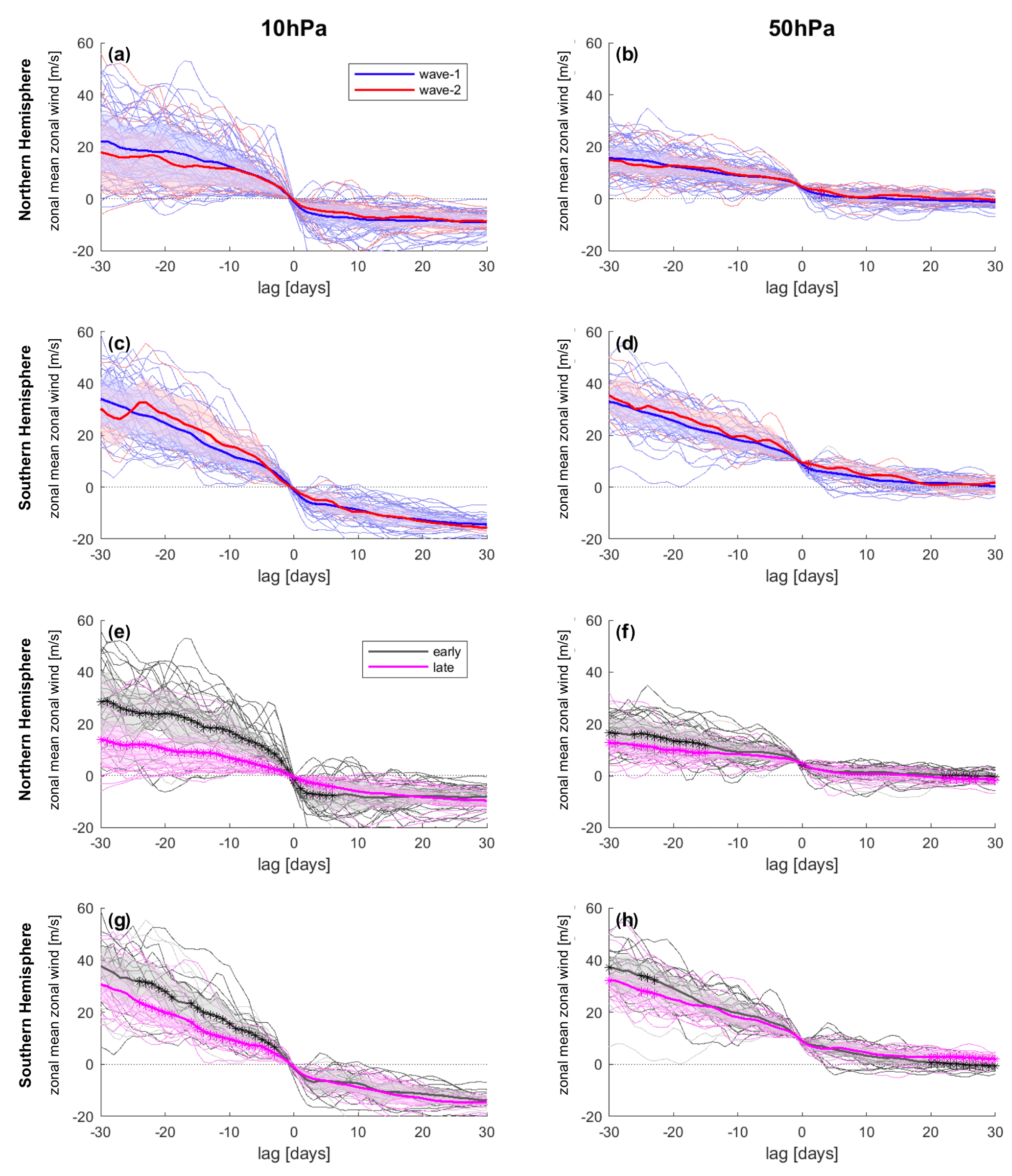
Figure 6Composites of zonal-mean zonal wind (m s−1) at 60∘ latitude and 10 hPa (a, c, e, g) and 50 hPa (b, d, f, h) for the NH (a, b, e, f) and the SH (c, d, g, h) for 1958–2019 (NH) and 1979–2019 (SH) for lags of −30 to +30 d around all final warming event dates defined at the indicated level. (a–d) Thin blue (red) lines correspond to a wave-1 (wave-2) classification. Thin gray lines (if applicable) correspond to FSW events unclassified by wavenumber. The bold blue (red) lines indicate the average of all events classified as wave-1 (wave-2) at the depicted level. The blue (red) shading indicates the area between the 25th and 75th percentile for the wave-1 (wave-2) classification. (e–h) Same as (a–d) but for early (black) vs. late (pink) FSW events; see text for definition. Thin gray lines correspond to FSW events classified as neither early nor late at the depicted level. Stars denote lags for which the composites for wave-1 and wave-2 or early and late events, respectively, are significantly different from each other at the 95 % level according to a t test.
In order to obtain a better comparison of the behavior of the zonal-mean zonal winds around the FSW event for the different wave classifications, Fig. 6 shows a composite of zonal-mean zonal wind for the month before and after the FSW using the date at either 10 hPa (Fig. 6a, c, e, and g) or 50 hPa (Fig. 6b, d, f, and h). The wind speeds about a month before the FSW event are weaker in the NH as compared to the SH (e.g., compare Figs. 6a and b with c and d). In the NH the winds can already exhibit values close to zero within the month before the FSW event, while in the SH the winds are significantly stronger in the month before the event. The average decrease in wind speed between the average over lags of −30 to −11 d before the FSW event and days 11 to 30 after the event is 25.2 m s−1 (36.7 m s−1) for the NH (SH) at 10 hPa. Further down at 50 hPa, these values are smaller, i.e., 12.8 m s−1 (24.8 m s−1) for the NH (SH). No significant differences are found in wind speed between wave-1 and wave-2 classifications. This suggests that, though the different wave geometries are clearly associated with asymmetries in the geopotential heights (Fig. 5), the wave geometry has little influence on the strength of the zonal-mean stratospheric wind changes.
We then compare this behavior to early vs. late FSW events. Early FSW events are associated with a stronger deceleration of the winds as compared to late FSW events at all levels and in both hemispheres due to the seasonally stronger winds earlier in the season (Fig. 6e–h). In the NH, the winds are significantly weaker before early FSW events at 50 hPa as compared to 10 hPa, while for late events, the deceleration is weaker at both levels. The decrease in wind speed between the average over lags of −30 to −11 d before the FSW event and days 11 to 30 after the event is 31.4 m s−1 (13.3 m s−1) at 10 (50) hPa for early events. For late events, the corresponding values are 18.8 m s−1 (10.8 m s−1) at 10 (50) hPa. In the SH the winds exhibit similar strengths before the FSW event at both 10 and 50 hPa, although the deceleration at the time of the FSW event is stronger at 10 hPa compared to 50 hPa. The decrease in wind speed between the average over lags of −30 to −11 d before the FSW event and days 11 to 30 after the event is 39.3 m s−1 (28.3 m s−1) at 10 (50) hPa for early events. For late events, the corresponding values are 33.4 m s−1 (22.8 m s−1) at 10 (50) hPa. The wind speeds at 10 hPa between early and late events are significantly different from each other for most lags before the FSW event, while at 50 hPa the winds speeds are significantly different for early vs. late events only at lags around −20 d or longer. After the FSW event, significant differences can only be detected between early and late events for the first few days at 10 hPa in the NH.
To investigate the influence of final warming wave geometry on total column ozone, we use the Bodeker Scientific filled total column ozone (TCO) database (Version 3.4) (Bodeker et al., 2020). This dataset combines measurements from multiple satellite-based instruments and fills missing data with a machine-learning-based method to create a temporally and spatially gap-free database of total column ozone from 31 October 1978 to 31 December 2016. We also compared these results to the same analysis using ERA-interim ozone at the 500 K isentrope (lower stratosphere), and the results were very similar (not shown). TCO anomalies are calculated based on the 1979–2016 daily climatology.

Figure 7Composite total column ozone anomaly (Dobson units) averaged over the 10 d prior to FSWs at 10 hPa for (a–e) the NH and (f–j) the SH. Panels show the composites based on (a, f) all events from 1979–2016 (the period of the TCO dataset), (b, g) wave-1 or (d, i) wave-2 classification, or (c, h) early or (e, j) late classification. Stippling in (a, f) indicates regions where the anomaly composites are significantly different from zero at the 95 % confidence level according to a two-tailed t test; stippling in other panels shows where composites are significantly different from each other (e.g., wave-1 vs. wave-2, early vs. late) using a t test for two samples of unequal variance.
Figure 7a–e show the NH TCO anomalies (from 1979–2016, the period of the ozone dataset) 10 d prior to the final warming for the 10 hPa FSW dates and for different classifications. A corresponding figure for the 50 hPa FSW dates is shown in the Appendix (Fig. A1), but we found in both hemispheres that the differences in TCO anomalies tied to wave geometry were more apparent for 10 hPa FSW dates. While spatial patterns are similar, TCO anomalies are generally weaker and less significant for FSWs at 50 hPa, likely because the vortex is smaller and potential gradients are weaker later in the season, and particularly for the NH, more of the ozone within the vortex has mixed with midlatitude air (Manney et al., 1994).
In the NH, negative TCO anomalies over northern Eurasia and positive TCO anomalies over Canada occur prior to wave-1 FSWs. This pattern closely matches the composite geometry of the vortex (Fig. 5a). The TCO anomalies prior to wave-2 FSWs show some wave-2 structure but more generally show positive TCO anomalies across the middle to high latitudes. Thus there are broad large-scale differences in TCO anomalies just prior to wave-1 and wave-2 NH FSWs which are statistically significant over Europe and Asia. Early NH FSWs defined at 10 hPa show significantly more positive TCO anomalies over the Pacific North American region compared to late FSWs. Early FSWs also exhibit negative anomalies over central Eurasia, echoing wave-1 events, but since late FSWs also show weakly negative TCO anomalies over northern Europe, the differences are less significant over Eurasia compared to the wave-1 vs. wave-2 differences.
In the SH (Fig. 7f–j), the TCO anomalies also closely mirror the geopotential height anomaly composites (Fig. 5i, k, m, and o), with negative (positive) TCO anomalies occurring over the Weddell Sea (east Antarctica) prior to wave-1 FSWs and negative (positive) TCO anomalies over the Amundsen-Ross seas (South Atlantic) prior to wave-2 FSWs. The differences in TCO anomalies between wave-1 and wave-2 FSWs are significant over most of the South Atlantic and South Pacific extratropical regions. Similar but much weaker TCO anomalies are seen following wave-1 and wave-2 events for FSWs defined at 50 hPa (Fig. A1b and d). Early FSWs show robust positive TCO anomalies, while late FSWs show robust negative TCO anomalies corresponding to significant differences in TCO anomalies over Antarctica. These differences likely reflect the fact that late events in the SH tend to occur in years with strong ozone depletion (Fig. 2) that further strengthen the vortex winds and allow the vortex to persist longer.
We have shown that both the wave geometry and timing of the event can play a role in the evolution of springtime TCO anomalies, which may have implications for ecosystems and human health due to increased ultraviolet (UV) radiation exposure (Barnes et al., 2019) or stratosphere-to-troposphere ozone transport (Albers et al., 2018). For example, prior to wave-1 and early NH FSWs there are widespread negative TCO anomalies over Eurasia and positive TCO anomalies over North America that are shifted off the pole towards more populated areas, compared to wave-2 and late NH FSWs.
There are observed differences in the NH surface impacts following displacement and split-type SSW events (Mitchell et al., 2013), though the robustness of these impacts is debated (Maycock and Hitchcock, 2015; Hall et al., 2021; White et al., 2021). To see if such differences exist following different geometries or timings of final warmings, we next investigate potential differences in the surface impact for different types of FSW events. Figure 8 shows the composite response for wave-1 and wave-2 (and early and late) FSWs for linearly detrended 500 hPa geopotential height anomalies for days 7–30 after the 50 hPa FSW event dates. A comparable figure is shown in the Appendix for 10 hPa dates (Fig. A2). The composites based on the 50 hPa dates are highlighted here because (1) changes of the vortex in the lower stratosphere have been linked more closely with changes in tropospheric circulation (Maycock and Hitchcock, 2015), and (2) the surface responses are more similar to known patterns associated with stratosphere–troposphere coupling following FSWs. The detrending was applied to account for possible trends in the storm tracks but does not qualitatively change the results.
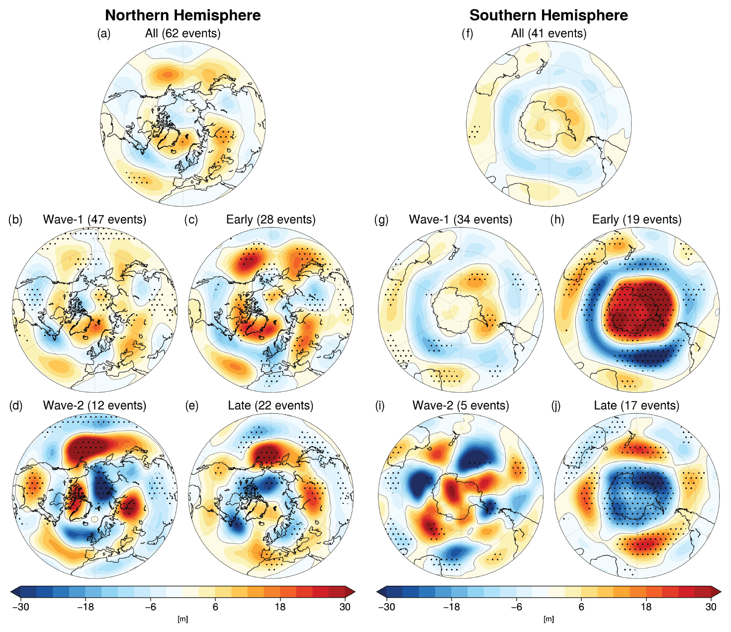
Figure 8Composite of the linearly detrended 500 hPa geopotential height anomalies (m) from JRA-55 data for (a, f) all FSW events based on the 50 hPa dates and classified as (b, g) wave-1, (d, i) wave-2, (c, h) early, or (e, j) late averaged over the 7–30 d after the central FSW date (i.e., lags of 7–30 d) for (a–e) the NH and (f–j) the SH extratropics. Stippling in (a, f) indicates regions where the anomaly composites are significantly different from zero at the 95 % confidence level according to a t test, while stippling in other panels shows where composites are significantly different from each other (e.g., wave-1 vs. wave-2, early vs. late) according to a 1000-sample bootstrap analysis (with replacement).
The average over all NH FSW events (Fig. 8a) shows a negative NAO-like structure with a high geopotential anomaly over Greenland and a low geopotential anomaly over Europe and the adjacent North Atlantic region. A positive geopotential height anomaly is observed in the North Pacific. When dividing the response between wave-1 and wave-2 (Fig. 8b and d), the negative NAO response persists for both types of events, but the response over North America is opposite between wave-1 and wave-2 events, with a positive (negative) anomaly over Canada for wave-1 (wave-2) events and the opposite response over the southern United States. Wave-2 events also show stronger positive anomalies over the North Pacific that are significantly different from wave-1 events. Early and late FSWs also show opposing but less significant differences across North America (Fig. 8c and e), but there are more significant differences in the circulation response over Eurasia compared to wave-1 vs. wave-2 events.
In the SH, anomalously high geopotential heights are found across Antarctica surrounded by anomalously low geopotential heights over the Southern Ocean in the average for all events (Fig. 8f), which resembles the negative phase of the Southern Annular Mode (SAM). The same pattern is apparent following both wave-1 and wave-2 events (Fig. 8g and i), though the wave-2 composite is noisy due to few samples. The surface impacts following FSWs are clearly dominated by the timing, not the wave geometry, of the FSW (Fig. 8h and j). Early FSWs show a significantly more negative SAM pattern compared to late FSWs which show a positive SAM pattern. Importantly, averaging over all events yields insignificant circulation anomalies (panel f), but this apparent lack of response arises from the cancellation of significant differences between early and late events. Overall, greater ozone loss in early austral spring leads to a colder vortex that persists longer (Fig. 2) and keeps ozone anomalously low until the FSW (Fig. 7j), resulting in a positive SAM and poleward-shifted jet stream into austral summer. Our results support findings that ozone hole recovery since 2000 has reversed circulation trends due to ozone depletion (Banerjee, Antara et al., 2020) towards earlier FSWs and a more negative SAM.
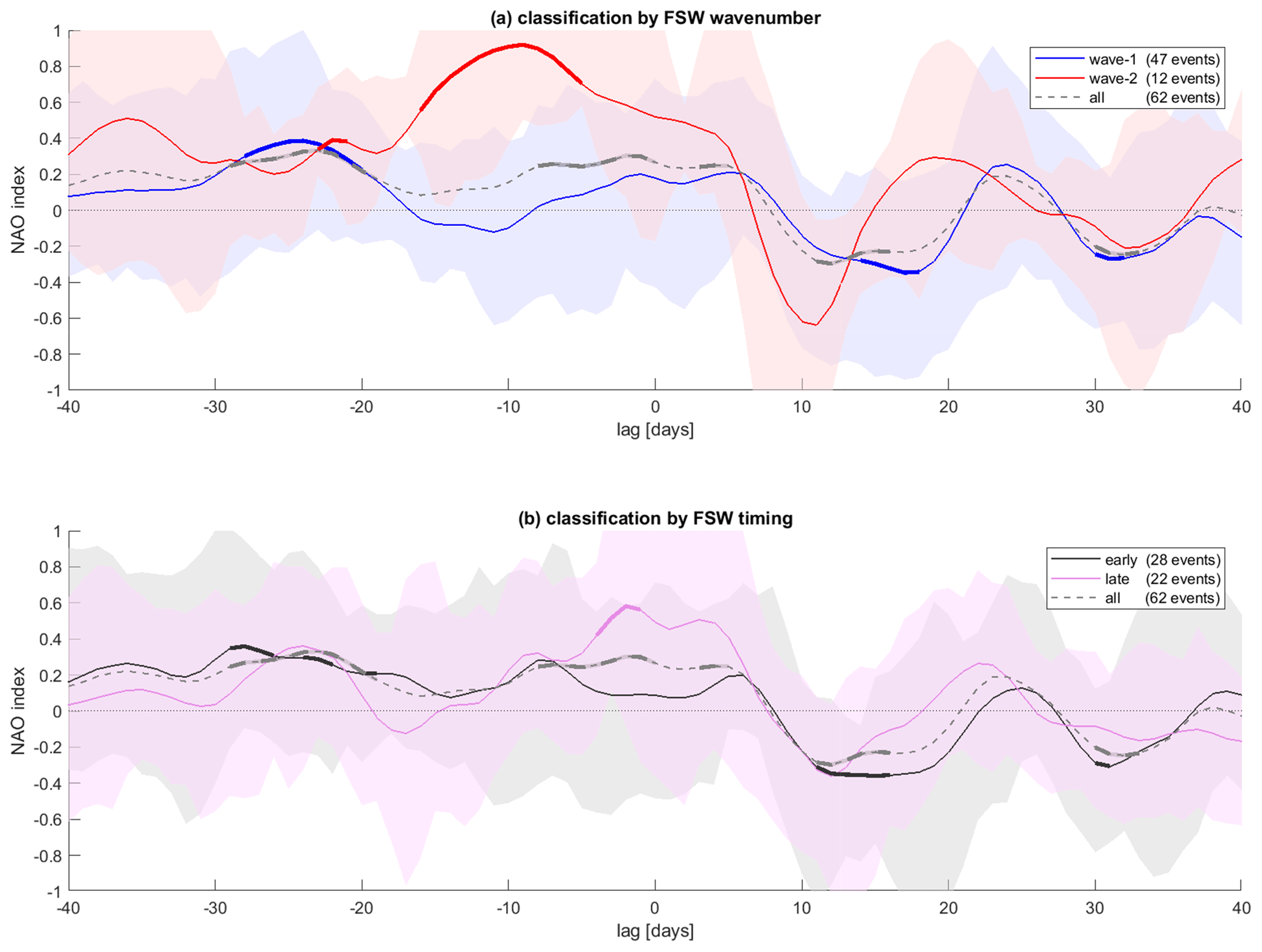
Figure 9Composite of the NAO index (using a 3 d running mean) for lags of −40 to +40 d around the final warming dates at 50 hPa for 1958–2019. (a) The blue (red) lines indicate the average values for the wave-1 (wave-2) classifications, respectively. The dashed gray line is the average over all FSW events from 1958–2019, including unclassified events. Bold parts of the lines indicate values significantly different from zero at the 95 % level according to a t test. The blue (red) shading indicates the 25th and 75th percentiles for the wave-1 (wave-2) classification. (b) Same as (a) but for early (black) vs. late (purple) FSW events.
Since the surface signal over the North Atlantic tends to show a structure reminiscent of the negative phase of the NAO (Fig. 8a), we also composite the NAO index (obtained from the Climate Prediction Center) for the period 1958–2019 using the 50 hPa FSW dates (Fig. 9a). The NAO experiences a decrease from significantly positive values before the FSW event to values close to zero or negative starting within a week after the event. Both wave-1 and wave-2 FSW events experience a tendency towards a negative NAO after the central day of the event, with on average consistently positive NAO values in the 40 d before the event. Values significantly different from zero are observed primarily for wave-1 events for lags between 5 and 20 d before the FSW event. Wave-2 events show larger variability, especially after the FSW event, likely due to the smaller sample size as compared to wave-1 events. A similar picture emerges when compositing the NAO for early vs. late events (Fig. 9b). Both early and late FSW events exhibit a drop in the NAO from positive to negative values roughly a week after the FSW event. Late events show more variability than early events.
Both sudden stratospheric warming events in the middle of winter and final stratospheric warming events that mark the end of winter in the stratosphere are characterized by a similar evolution and are often classified by the same metrics, i.e., when the zonal-mean zonal winds of the polar vortex fall below some threshold. However, in order to characterize their evolution further, different measures are used. The most dominant classification for midwinter sudden stratospheric warmings is by their wave geometry into split and displacement events. FSWs, on the other hand, have so far not been classified by geometry but only by their timing or vertical evolution. This difference in the classification between midwinter and end-of-winter polar vortex breakdowns is likely due to the notion that a wave geometry cannot always be identified for FSW events, especially for events that occur later in spring and that are more radiatively driven. We show here that final warmings can almost exclusively be classified with regard to their geometrical wave structure. This geometrical structure is present even for most late events. A detailed classification of wave geometry using FSWs detected at two different pressure levels and for two different reanalysis products is provided.
Defining the final warming date at 50 vs. 10 hPa yields a much more significant shift in the timing in the SH as compared to the NH. In particular, using the 50 hPa dates more clearly captures ozone-related trends in the timing of the SH FSWs. On the other hand, the interannual variability in FSW dates at 10 and 50 hPa is significantly correlated in both hemispheres. Our analysis suggests that, depending on the question being explored, there could be valid reasons for using either the 10 or 50 hPa dates. For example, for SSWs the 10 hPa level has been found to be optimal for detecting dynamic changes in the stratospheric circulation, whereas the 50 hPa level shows stronger linkages to surface impacts (Butler and Gerber, 2018). Here, we noted a more significant relationship of wave geometry to TCO anomalies using the 10 hPa dates but a more expected tropospheric response when using the 50 hPa dates.
Weaker westerly winds in spring allow for more vertical propagation of wave-2 and even wave-3 into the stratosphere. Similar to SSWs, more events are characterized as wave-1 events as compared to wave-2 events in both hemispheres. Wave-3 plays a more significant role in the NH stratosphere during the FSW compared to midwinter SSW events, when wave-3 is generally not able to propagate into the strong vortex winds present prior to SSWs. One NH event in 2009 was classified as a wave-3 event, and several other events show clear wave-3 structure even in the SH.
To bring together the influence of FSW wave geometry on the polar vortex, TCO anomalies, and tropospheric impacts, here we summarize the composite impacts from each type of classification. Wave-1 events shift the polar vortex off the pole preferentially towards Eurasia in the NH and the Weddell Sea in the SH. This is associated with anomalously high stratospheric heights over Canada in the NH and over east Antarctica in the SH. The vortex shift is associated with anomalously low total column ozone in the region where the ozone-poor vortex air shifts towards and anomalously high total column ozone in the region it moves away from. Wave-1 events are followed in the NH by a negative NAO-like pattern in the North Atlantic, positive 500 hPa height anomalies over Canada, and negative 500 hPa height anomalies over the United States.
Wave-2 events in the NH generally consist of an elongated or split vortex preferentially over Canada and eastern Asia, with anomalously high stratospheric heights over the North Pacific and European sectors. In the SH, the vortex evolution is less consistent for wave-2, but on average there are anomalously high stratospheric heights south of Africa and negative heights over the South Pacific. Wave-2 events are associated with broadly positive total column ozone anomalies in both hemispheres. For surface impacts, NH wave-2 events are followed by anomalously positive 500 hPa height anomalies over the North Pacific and United States, oppositely signed to wave-1 events, though the negative NAO pattern is consistent.
From our results, it is evident that the FSW wave geometry could be relevant for understanding and predicting the evolution of total column ozone anomalies in spring. In particular, wave-1 events tend to be associated with more widespread negative TCO anomalies prior to the FSW than wave-2 events in both hemispheres. This may be because, while wave-2 events tend to be associated with elongation and possible splitting over the pole, wave-1 events displace the vortex equatorward into more sunlit regions. Still, the timing of the FSW is also very important; in the SH, differences in polar cap TCO anomalies for early and late events are likely associated with chemistry–climate feedbacks that play a central role in stratosphere–troposphere coupling in austral spring. Consideration of both the timing and geometry of the FSW in both hemispheres may be important for how much stratospheric ozone is available to be transported via deep stratospheric intrusions to the surface in spring (Albers et al., 2018; Breeden et al., 2020).
While there are some indications of the modulation of tropospheric impacts by FSW wave geometry, in general FSWs of either wave classification are followed by a shift towards the negative phase of the NAO in the NH and the SAM in the SH. We did not attempt to identify causes for the different surface response over, for example, North America, which could be linked to tropospheric variability leading up to the FSWs, the more direct influence of the stratospheric wave geometry on the underlying tropospheric circulation, or to other large-scale climate patterns like El Niño–Southern Oscillation (Domeisen et al., 2019) or decadal variability. These signals may also arise due to sampling given the small number of events available in the historical record; further testing with long model simulations may reveal non-significant differences (e.g., Maycock and Hitchcock, 2015). Tropospheric impacts are strongly tied to the timing of the FSW in the SH, where the tropospheric height pattern is nearly the mirror opposite for early and late FSWs. These differences are likely related to the trends associated with ozone depletion and recovery that have been linked both to trends in the timing of SH FSWs and to changes in atmospheric circulation.
The ability to classify final stratospheric warming events by wave geometry points out similarities with midwinter sudden stratospheric warming events, while the greater importance of wave-3 for FSWs highlights the differences. We have shown that the structure of the stratospheric polar vortex as it weakens in spring can influence total column ozone and tropospheric impacts, suggesting that the wave geometry of FSWs may be important for improving predictive skill following these events. Whether the wave geometry characteristics of FSWs are well simulated in climate and forecast models, and if they are modulated by external forcings like increasing greenhouse gases, should be investigated.
Table A1Details of JRA-55 classification for 1979–2019 using NH final warming dates based on 60∘ N and 10 hPa. The two metrics determine the wavenumber (WN) with maximum mean amplitude and highest percent of days of maximum amplitude for the 10 d before the FSW, as described in Sect. 2. U=unclassified (methods did not agree according to the criterion outlined in Sect. 2).
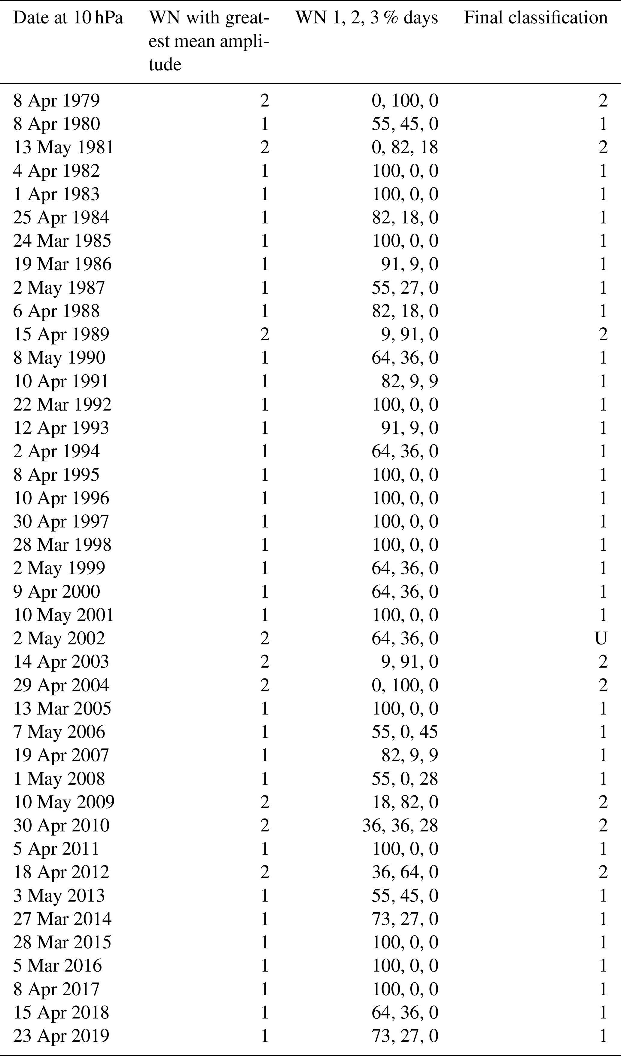

Figure A1Composite total column ozone anomaly (Dobson units) averaged over the 10 d prior to FSWs at 50 hPa for (a–e) the NH and (f–j) the SH. Panels show the composites based on (a, f) all events from 1979–2016 (the period of the TCO dataset), (b, g) wave-1 or (d, i) wave-2 classification, or (c, h) early or (e, j) late classification. Stippling in (a, f) indicates regions where the anomaly composites are significantly different from zero at the 95 % confidence level on a two-tailed t test; stippling in other panels shows where composites are significantly different from each other (e.g., wave-1 vs. wave-2, early vs. late) using a t test for two samples of unequal variance.
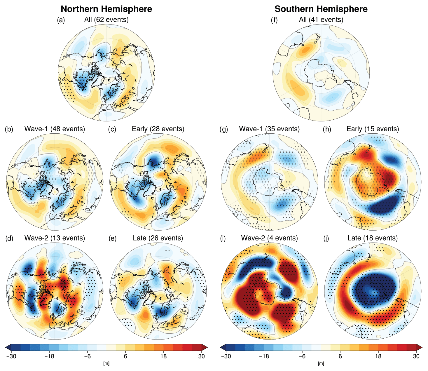
Figure A2Composite of the linearly detrended 500 hPa geopotential height anomalies (m) from JRA-55 data for (a, f) all FSW events based on the 10 hPa dates and classified as (b, g) wave-1, (d, i) wave-2, (c, h) early, or (e, j) late averaged over the 7–30 d after the central FSW date (i.e., lags of 7–30 d) for (a–e) the NH and (f–j) the SH extratropics. Stippling in (a, f) indicates regions where the anomaly composites are significantly different from zero at the 95 % confidence level according to a t test, while stippling in other panels shows where composites are significantly different from each other (e.g., wave-1 vs. wave-2, early vs. late) according to a 1000-sample bootstrap analysis (with replacement).
The ERA-interim Reanalysis data were obtained from the ECMWF data portal at https://apps.ecmwf.int/datasets/data/interim-full-daily/ (Berrisford et al., 2011). The JRA-55 data were obtained from the NCAR Research Data Archive at https://doi.org/10.5065/D6HH6H41 (Japan Meteorological Agency/Japan, 2013). The NAO index was obtained from the Climate Prediction Center at https://www.cpc.ncep.noaa.gov/products/precip/CWlink/pna/nao.shtml (National Oceanic and Atmospheric Administration, Climate Prediction Center, 2021). The total column ozone database was obtained from https://doi.org/10.5281/zenodo.3908787 (Bodeker et al., 2020). We would like to thank Bodeker Scientific, funded by the New Zealand Deep South National Science Challenge, for providing the combined NIWA-BS total column ozone database.
The authors together initiated and designed the study. Both authors contributed to figures, and both contributed to the writing.
The authors declare that they do not have any competing interests.
The authors thank Darryn Waugh, Nick Byrne, and an anonymous reviewer, as well as the co-editor Yang Zhang, for their helpful comments during the discussion phase.
Amy H. Butler has been supported by the National Science Foundation (grant no. 1756958) and Daniela I. V. Domeisen by the Swiss National Science Foundation (grant no. PP00P2_170523).
This paper was edited by Yang Zhang and reviewed by Darryn Waugh and one anonymous referee.
Afargan-Gerstman, H. and Domeisen, D. I. V.: Pacific Modulation of the North Atlantic Storm Track Response to Sudden Stratospheric Warming Events, Geophys. Res. Lett., 47, 18–10, https://doi.org/10.1029/2019GL085007, 2020. a
Albers, J. R., Perlwitz, J., Butler, A. H., Birner, T., Kiladis, G. N., Lawrence, Z. D., Manney, G. L., Langford, A. O., and Dias, J.: Mechanisms Governing Interannual Variability of Stratosphere-to-Troposphere Ozone Transport, J. Geophys. Res.-Atmos., 123, 234–260, 2018. a, b
Ayarzagüena, B. and Serrano, E.: Monthly Characterization of the Tropospheric Circulation over the Euro-Atlantic Area in Relation with the Timing of Stratospheric Final Warmings, J. Climate, 22, 6313–6324, 2009. a, b
Baldwin, M. P., Ayarzaguena, B., Birner, T., Butchart, N., Butler, A. H., Charlton-Perez, A. J., Domeisen, D. I. V., Garfinkel, C. I., Garny, H., Gerber, E. P., Hegglin, M. I., Langematz, U., and Pedatella, N. M.: Sudden Stratospheric Warmings, Rev. Geophys., 59, 27.1–37, 2021. a, b
Bancalá, S., Krüger, K., and Giorgetta, M.: The preconditioning of major sudden stratospheric warmings, J. Geophys. Res., 117, D04101, https://doi.org/10.1029/2011JD016769, 2012. a, b, c
Banerjee, A., Fyfe, J. C, Polvani, L. M., Waugh, D., and Chang, K-L.: A pause in Southern Hemisphere circulation trends due to the Montreal Protocol., Nat. Geosci., 579, 544–548, 2020. a, b
Barnes, P. W., Williamson, C. E., Lucas, R. M., Robinson, S. A., Madronich, S., Paul, N. D., Bornman, J. F., Bais, A. F., Sulzberger, B., Wilson, S. R., Andrady, A. L., McKenzie, R. L., Neale, P. J., Austin, A. T., Bernhard, G. H., Solomon, K. R., Neale, R. E., Young, P. J., Norval, M., Rhodes, L. E., Hylander, S., Rose, K. C., Longstreth, J., Aucamp, P. J., Ballaré, C. L., Cory, R. M., Flint, S. D., de Gruijl, F. R., Häder, D.-P., Heikkilä, A. M., Jansen, M. A. K., Pandey, K. K., Robson, T. M., Sinclair, C. A., Wängberg, S.-Å., Worrest, R. C., Yazar, S., Young, A. R., and Zepp, R. G.: Ozone depletion, ultraviolet radiation, climate change and prospects for a sustainable future, Nature Sustainability, 2, 569–579, 2019. a
Barriopedro, D. and Calvo, N.: On the Relationship between ENSO, Stratospheric Sudden Warmings, and Blocking, J. Climate, 27, 4704–4720, 2014. a, b, c, d, e, f
Berrisford, P., Dee, D. P., Poli, P., Brugge, R., Fielding, M., Fuentes, M., Kållberg, P. W., Kobayashi, S., Uppala, S., and Simmons, A.: The ERA-Interim archive Version 2.0, ERA Report Series, https://www.ecmwf.int/node/8174 (last access: 21 May 2021). a
Black, R., McDaniel, B., and Robinson, W. A.: Stratosphere-troposphere coupling during spring onset, J. Climate, 19, 4891–4901, 2006. a, b, c
Black, R. X. and McDaniel, B.: Interannual Variability in the Southern Hemisphere Circulation Organized by Stratospheric Final Warming Events, J. Atmos. Sci., 64, 2968–2974, 2007a. a, b, c, d
Black, R. X. and McDaniel, B. A.: The dynamics of northern hemisphere stratospheric final warming events, J. Atmos. Sci., 64, 2932–2946, 2007b. a, b, c
Bodeker, G. E., Kremser, S., and Tradowsky, J. S.: BS Filled Total Column Ozone Database (Version 3.4) [data set], https://doi.org/10.5281/zenodo.3908787, 2020. a, b, c
Breeden, M. L., Butler, A. H., Albers, J. R., Sprenger, M., and Langford, A. O.: The spring transition of the North Pacific jet and its relation to deep stratosphere-to-troposphere mass transport over western North America, Atmos. Chem. Phys., 21, 2781–2794, https://doi.org/10.5194/acp-21-2781-2021, 2021. a
Butler, A. H. and Gerber, E. P.: Optimizing the definition of a sudden stratospheric warming, J. Climate, 31, 2337–2344, 2018. a, b, c
Butler, A. H., Seidel, D. J., Hardiman, S. C., Butchart, N., Birner, T., and Match, A.: Defining sudden stratospheric warmings, B. Am. Meteorol. Soc., 96, 1913–1928, 2015. a
Butler, A. H., Sjoberg, J. P., Seidel, D. J., and Rosenlof, K. H.: A sudden stratospheric warming compendium, Earth Syst. Sci. Data, 9, 63–76, https://doi.org/10.5194/essd-9-63-2017, 2017. a
Butler, A. H., Charlton-Perez, A., Domeisen, D. I. V., Simpson, I., and Sjoberg, J.: Predictability of Northern Hemisphere final stratospheric warmings and their surface impacts, Geophys. Res. Lett., 46, https://doi.org/10.1029/2019GL083346, 2019. a, b
Byrne, N. J. and Shepherd, T. G.: Seasonal Persistence of Circulation Anomalies in the Southern Hemisphere Stratosphere and Its Implications for the Troposphere, J. Climate, 31, 3467–3483, 2018. a
Byrne, N. J., Shepherd, T. G., Woollings, T., and Plumb, R. A.: Nonstationarity in Southern Hemisphere Climate Variability Associated with the Seasonal Breakdown of the Stratospheric Polar Vortex, J. Climate, 30, 7125–7139, 2017. a, b
Byrne, N. J., Shepherd, T. G., and Polichtchouk, I.: Subseasonal-to-Seasonal Predictability of the Southern Hemisphere Eddy-Driven Jet During Austral Spring and Early Summer, J. Geophys. Res.-Atmos., 124, 6841–6855, 2019. a
Calvo, N., Polvani, L. M., and Solomon, S.: On the surface impact of Arctic stratospheric ozone extremes, Environ. Res. Lett., 10, https://doi.org/10.1088/1748-9326/10/9/094003, 2015. a
Charlton, A. and Polvani, L. M.: A new look at stratospheric sudden warmings. Part I: Climatology and modeling benchmarks, J. Climate, 20, 449–469, 2007. a, b, c, d
Charlton, A., O'Neill, A., Lahoz, W., and Berrisford, P.: The splitting of the stratospheric polar vortex in the Southern Hemisphere, September 2002: Dynamical evolution, J. Atmos. Sci., 62, 590–602, 2005. a
Charlton-Perez, A. J., Ferranti, L., and Lee, R. W.: The influence of the stratospheric state on North Atlantic weather regimes, Q. J. Roy. Meteor. Soc., 144, 1140–1151, 2018. a
Charney, J. and Drazin, P.: Propagation of planetary-scale disturbances from the lower into the upper atmosphere, J. Geophys. Res., 66, 83–109, 1961. a, b
Chipperfield, M. P. and Jones, R. L.: Relative influences of atmospheric chemistry and transport on Arctic ozone trends, Nature, 400, 551–554, 1999. a
Coy, L., Nash, E. R., and Newman, P. A.: Meteorology of the polar vortex: Spring 1997, Geophys. Res. Lett., 24, 2693–2696, 1997. a
Dee, D. P., Uppala, S. M., Simmons, A. J., Berrisford, P., Poli, P., Kobayashi, S., Andrae, U., Balmaseda, M. A., Balsamo, G., Bauer, P., Bechtold, P., Beljaars, A. C. M., van de Berg, L., Bidlot, J., Bormann, N., Delsol, C., Dragani, R., Fuentes, M., Geer, A. J., Haimberger, L., Healy, S. B., Hersbach, H., Holm, E. V., Isaksen, L., Kallberg, P., Köhler, M., Matricardi, M., McNally, A. P., Monge-Sanz, B. M., Morcrette, J.-J., Park, B.-K., Peubey, C., de Rosnay, P., Tavolato, C., Thepaut, J.-N., and Vitart, F.: The ERAInterim reanalysis: Configuration and performance of the data assimilation system, Q. J. Roy. Meteor. Soc., 137, 553–597, 2011. a
Domeisen, D. I. V.: Estimating the Frequency of Sudden Stratospheric Warming Events from Surface Observations of the North Atlantic Oscillation, J. Geophys. Res.-Atmos., 124, 3180–3194, https://doi.org/10.1029/2018JD030077, 2019. a, b
Domeisen, D. I. V. and Butler, A. H.: Stratospheric drivers of extreme events at the Earth's surface, Communications Earth & Environment, 1, 59, https://doi.org/10.1038/s43247-020-00060-z, 2020. a
Domeisen, D. I. V., Garfinkel, C. I., and Butler, A. H.: The Teleconnection of El Niño Southern Oscillation to the Stratosphere, Rev. Geophys., 57, 5–47, https://doi.org/10.1029/2018RG000596, 2019. a
Domeisen, D. I. V., Butler, A. H., Charlton-Perez, A. J., Ayarzaguena, B., Baldwin, M. P., Dunn Sigouin, E., Furtado, J. C., Garfinkel, C. I., Hitchcock, P., Karpechko, A. Y., Kim, H., Knight, J., Lang, A. L., Lim, E.-P., Marshall, A., Roff, G., Schwartz, C., Simpson, I. R., Son, S.-W., and Taguchi, M.: The Role of the Stratosphere in Subseasonal to Seasonal Prediction: 1. Predictability of the Stratosphere, J. Geophys. Res.-Atmos., 125, 1–17, 2020. a
Gerber, E. P. and Martineau, P.: Quantifying the variability of the annular modes: reanalysis uncertainty vs. sampling uncertainty, Atmos. Chem. Phys., 18, 17099–17117, https://doi.org/10.5194/acp-18-17099-2018, 2018. a
Gerber, E. P., Martineau, P., Ayarzagüena, B., Barriopedro, D., Bracegirdle, T. J., Butler, A. H., Calvo, N., Hardiman, S. C., Hitchcock, P., Iza, M., Langematz, U., Lua, H., Marshall, G., Orr, A., Palmeiro, F. M., Son, S.-W., and Taguchi, M.: Extratropical stratosphere-troposphere coupling, in: Stratosphere-troposphere processes and their role in climate (SPARC) reanalysis intercomparison project (S-RIP), edited by: Fujiwara, M., Manney, G. L., Gray, L., and Wright, J. S., chap. 6, SPARC, Oberpfaffenhofen, Germany, in press, 2021. a, b
Haigh, J. D. and Roscoe, H. K.: The Final Warming Date of the Antarctic Polar Vortex and Influences on its Interannual Variability, J. Climate, 22, 5809–5819, 2009. a
Hall, R. J., Mitchell, D. M., Seviour, W. J. M., and Wright, C. J.: Tracking the stratosphere-to-surface impact of Sudden Stratospheric Warmings, J. Geophys. Res.-Atmos., 126, e2020JD033881, 1–47, 2021. a
Hardiman, S. C., Butchart, N., Charlton-Perez, A. J., Shaw, T. A., Akiyoshi, H., Baumgaertner, A., Bekki, S., Braesicke, P., Chipperfield, M., Dameris, M., Garcia, R. R., Michou, M., Pawson, S., Rozanov, E., and Shibata, K.: Improved predictability of the troposphere using stratospheric final warmings, J. Geophys. Res., 116, 6313, https://doi.org/10.1029/2011JD015914, 2011. a, b, c
Harvey, V. L., Pierce, R. B., Fairlie, T. D., and Hitchman, M. H.: A climatology of stratospheric polar vortices and anticyclones, J. Geophys. Res.-Atmos., 107, https://doi.org/10.1029/2001JD001471, 2002. a
Hu, J. G., Ren, R. C., and Xu, H. M.: Occurrence of Winter Stratospheric Sudden Warming Events and the Seasonal Timing of Spring Stratospheric Final Warming, J. Atmos. Sci., 71, 2319–2334, 2014. a
Ialongo, I., Sofieva, V., Kalakoski, N., Tamminen, J., and Kyrölä, E.: Ozone zonal asymmetry and planetary wave characterization during Antarctic spring, Atmos. Chem. Phys., 12, 2603–2614, https://doi.org/10.5194/acp-12-2603-2012, 2012. a
Ivy, D. J., Solomon, S., Calvo, N., and Thompson, D. W. J.: Observed connections of Arctic stratospheric ozone extremes to Northern Hemisphere surface climate, Environ. Res. Lett., 12, 024004, https://doi.org/10.1029/2001JD001471, 2017. a
Japan Meteorological Agency/Japan: JRA-55: Japanese 55-year Reanalysis, Daily 3-Hourly and 6-Hourly Data, Research Data Archive at the National Center for Atmospheric Research, Computational and Information Systems Laboratory [data set], https://doi.org/10.5065/D6HH6H41 (last access: 21 May 2021), 2013, updated monthly. a
Karpechko, A. Y.: Predictability of Sudden Stratospheric Warmings in the ECMWF Extended-Range Forecast System, Mon. Weather Rev., 146, 1063–1075, 2018. a
Karpechko, A. Y., Hitchcock, P., Peters, D. H. W., and Schneidereit, A.: Predictability of downward propagation of major sudden stratospheric warmings, Q. J. Roy. Meteor. Soc., 104, 30937, https://doi.org/10.1002/qj.3017, 2017. a
Karpechko, A. Y., Perez, A. C., Balmaseda, M., Tyrrell, N., and Vitart, F.: Predicting Sudden Stratospheric Warming 2018 and its Climate Impacts with a Multi-Model Ensemble, Geophys. Res. Lett., 45, 2018GL081091, https://doi.org/10.1029/2018GL081091, 2018. a
Kobayashi, S., Ota, Y., Harada, Y., Ebita, A., Moriya, M., Onoda, H., Onogi, K., Kamahori, H., Kobayashi, C., Endo, H., Miyaoka, K., and Takahashi, K.: The JRA-55 Reanalysis: General Specifications and Basic Characteristics, J. Meteorol. Soc. Jpn. Ser. II, 93, 5–48, https://doi.org/10.2151/jmsj.2015-001, 2015. a
Kodera, K., Mukougawa, H., Maury, P., Ueda, M., and Claud, C.: Absorbing and reflecting sudden stratospheric warming events and their relationship with tropospheric circulation, J. Geophys. Res.-Atmos., 121, 80–94, 2016. a
Kravchenko, V. O., Evtushevsky, O. M., Grytsai, A. V., Klekociuk, A. R., Milinevsky, G. P., and Grytsai, Z. I.: Quasi-stationary planetary waves in late winter Antarctic stratosphere temperature as a possible indicator of spring total ozone, Atmos. Chem. Phys., 12, 2865–2879, https://doi.org/10.5194/acp-12-2865-2012, 2012. a
Lawrence, Z. D., Perlwitz, J., Butler, A. H., Manney, G. L., Newman, P. A., Lee, S. H., and Nash, E. R.: The Remarkably Strong Arctic Stratospheric Polar Vortex of Winter 2020: Links to Record-Breaking Arctic Oscillation and Ozone Loss, J. Geophys. Res.-Atmos., 125, 1–29, 2020. a
Lim, E. P., Hendon, H. H., and Thompson, D. W. J.: Seasonal Evolution of Stratosphere-Troposphere Coupling in the Southern Hemisphere and Implications for the Predictability of Surface Climate, J. Geophys. Res.-Atmos., 123, 12002–12016, 2018. a
Manney, G. L. and Lawrence, Z. D.: The major stratospheric final warming in 2016: dispersal of vortex air and termination of Arctic chemical ozone loss, Atmos. Chem. Phys., 16, 15371–15396, https://doi.org/10.5194/acp-16-15371-2016, 2016. a
Manney, G. L., Farrara, J. D., and Mechoso, C. R.: The behavior of wave 2 in the Southern Hemisphere stratosphere during late winter and early spring, J. Atmos. Sci., 48, 976–998, 1991. a
Manney, G. L., Zurek, R. W., O'Neill, A., and Swinbank, R.: On the motion of air through the stratospheric polar vortex, J. Atmos. Sci., 51, 2973–2994, 1994. a
Matsuno, T.: Vertical Propagation of Stationary Planetary Waves in the Winter Northern Hemisphere, J. Atmos. Sci., 27, 871–883, 1970. a
Maycock, A. C. and Hitchcock, P.: Do split and displacement sudden stratospheric warmings have different annular mode signatures?, Geophys. Res. Lett., 42, 10943–10951, 2015. a, b, c
Mechoso, C. R., O'Neill, A., Pope, V. D., and Farrara, J. D.: A Study of the Stratospheric Final Warming of 1982 in the Southern-Hemisphere, Q. J. Roy. Meteor. Soc., 114, 1365–1384, 1988. a
Mitchell, D. M., Charlton-Perez, A. J., and Gray, L. J.: Characterizing the Variability and Extremes of the Stratospheric Polar Vortices Using 2D Moment Analysis, J. Atmos. Sci., 68, 1194–1213, 2011. a
Mitchell, D. M., Gray, L. J., Anstey, J., Baldwin, M. P., and Charlton-Perez, A. J.: The Influence of Stratospheric Vortex Displacements and Splits on Surface Climate, J. Climate, 26, 2668–2682, 2013. a
National Oceanic and Atmospheric Administration, Climate Prediction Center: The North Atlantic Oscillation index [data set], https://www.cpc.ncep.noaa.gov/products/precip/CWlink/pna/nao.shtml, last access: 21 May 2021. a
Newman, P. A.: The final warming and polar vortex disappearance during the Southern Hemisphere spring, Geophys. Res. Lett., 13, 1228–1231, 1986. a
Newman, P. A., Nash, E., and Rosenfield, J.: What controls the temperature of the Arctic stratosphere during the spring?, J. Geophys. Res., 106, 19999–20010, 2001. a
Plumb, R. A.: On the seasonal cycle of stratospheric planetary waves, Pure Appl. Geophys., 130, 233–242, 1989. a
Plumb, R. A.: Planetary waves and the extratropical winter stratosphere, in: The Stratosphere, Dynamics, Transport and Chemistry, 190, 23–41, Geophysical Monograph, American Geophysical Union, Washington, D. C., 2010. a
Randel, W.: The seasonal evolution of planetary waves in the Southern Hemisphere stratosphere and troposphere, Q. J. Roy. Meteor. Soc., 114, 1385–1409, 1988. a, b
Reichler, T., Kim, J., Manzini, E., and Kröger, J.: A stratospheric connection to Atlantic climate variability, Nat. Geosci., 5, 783–787, 2012. a
Rood, R. B. and Schoeberl, M. R.: Ozone transport by diabatic and planetary wave circulations on a β plane, J. Geophys. Res.-Atmos., 88, 8491–8504, 1983. a
Runde, T., Dameris, M., Garny, H., and Kinnison, D. E.: Classification of stratospheric extreme events according to their downward propagation to the troposphere, Geophys. Res. Lett., 43, 6665–6672, 2016. a
Salby, M. L. and Callaghan, P. F.: Influence of planetary wave activity on the stratospheric final warming and spring ozone, J. Geophys. Res.-Atmos., 112, 351, 2007. a
Savenkova, E. N., Kanukhina, A. Y., Pogoreltsev, A. I., and Merzlyakov, E. G.: Variability of the springtime transition date and planetary waves in the stratosphere, J. Atmos. Sol.-Terr. Phy., 90–91, 1–8, 2012. a, b
Scott, R. and Haynes, P.: The seasonal cycle of planetary waves in the winter stratosphere, J. Atmos. Sci., 59, 803–822, 2002. a
Seviour, W. J. M., Mitchell, D. M., and Gray, L. J.: A practical method to identify displaced and split stratospheric polar vortex events, Geophys. Res. Lett., 40, 5268–5273, 2013. a
Sheshadri, A., Plumb, R. A., and Domeisen, D. I. V.: Can the delay in Antarctic polar vortex breakup explain recent trends in surface westerlies?, J. Atmos. Sci., 71, 566–573, https://doi.org/10.1175/JAS-D-12-0343.1, 2014. a
Solomon, S.: Stratospheric ozone depletion: A review of concepts and history, Rev. Geophys., 37, 275–316, 1999. a
Solomon, S., Haskins, J., Ivy, D. J., and Min, F.: Fundamental differences between Arctic and Antarctic ozone depletion, P. Natl. Acad. Sci. USA, 111, 6220–6225, 2014. a
Son, S.-W., Purich, A., Hendon, H. H., Kim, B.-M., and Polvani, L. M.: Improved seasonal forecast using ozone hole variability?, Geophys. Res. Lett., 40, 6231–6235, 2013. a
Sun, L., Robinson, W. A., and Chen, G.: The role of planetary waves in the downward influence of stratospheric final warming events, J. Atmos. Sci., 68, 2826–2843, 2011. a
Taguchi, M.: Predictability of Major Stratospheric Sudden Warmings of the Vortex Split Type: Case Study of the 2002 Southern Event and the 2009 and 1989 Northern Events, J. Atmos. Sci., 71, 2886–2904, 2014. a
Taguchi, M.: Connection of predictability of major stratospheric sudden warmings to polar vortex geometry, Atmos. Sci. Lett., 17, 33–38, 2016. a
Thompson, D. W. J., Solomon, S., Kushner, P., England, M., Grise, K., and Karoly, D.: Signatures of the Antarctic ozone hole in Southern Hemisphere surface climate change, Nat. Geosci., 4, 741–749, 2011. a
Vargin, P. N., Kostrykin, S. V., Rakushina, E. V., Volodin, E. M., and Pogoreltsev, A. I.: Study of the Variability of Spring Breakup Dates and Arctic Stratospheric Polar Vortex Parameters from Simulation and Reanalysis Data, Izvestiya, Atmospheric and Oceanic Physics, 56, 458–469, 2020. a
Wang, T., Zhang, Q., Hannachi, A., Lin, Y., and Hirooka, T.: On the dynamics of the spring seasonal transition in the two hemispheric high-latitude stratosphere, Tellus A, 71, 1–18, 2019. a
Waugh, D. W.: Elliptical diagnostics of stratospheric polar vortices, Q. J. Roy. Meteor. Soc., 123, 1725–1748, 1997. a
Waugh, D. W. and Randel, W.: Climatology of Arctic and Antarctic polar vortices using elliptical diagnostics, J. Atmos. Sci., 56, 1594–1613, 1999. a, b
Waugh, D. W. and Rong, P. P.: Interannual variability in the decay of lower stratospheric Arctic vortices, J. Meteorol. Soc. Jpn., 80, 997–1012, 2002. a, b, c
Waugh, D. W., Randel, W. J., Pawson, S., Newman, P. A., and Nash, E. R.: Persistence of the lower stratospheric polar vortices, J. Geophys. Res.-Atmos., 104, 27191–27201, 1999. a, b
White, I. P., Garfinkel, C. I., Cohen, J., Jucker, M., and Rao, J.: The impact of split and displacement sudden stratospheric warmings on the troposphere, J. Geophys. Res.-Atmos., 126, e2020JD033989, https://doi.org/10.1029/2020JD033989, 2021. a
Zhang, Y., Li, J., and Zhou, L.: The Relationship between Polar Vortex and Ozone Depletion in the Antarctic Stratosphere during the Period 1979–2016, Adv. Meteorol., 2017, 1–12, 2017. a, b
Zhou, S., Gelman, M. E., Miller, A. J., and McCormack, J. P.: An inter-hemisphere comparison of the persistent stratospheric polar vortex, Geophys. Res. Lett., 27, 1123–1126, 2000. a
- Abstract
- Introduction
- Detection and classification of FSW events
- Relationship between geometry and dynamical behavior
- Implications for ozone distribution during spring onset
- Surface impacts
- Conclusions
- Appendix A
- Data availability
- Author contributions
- Competing interests
- Acknowledgements
- Financial support
- Review statement
- References
The requested paper has a corresponding corrigendum published. Please read the corrigendum first before downloading the article.
- Article
(8681 KB) - Full-text XML
- Abstract
- Introduction
- Detection and classification of FSW events
- Relationship between geometry and dynamical behavior
- Implications for ozone distribution during spring onset
- Surface impacts
- Conclusions
- Appendix A
- Data availability
- Author contributions
- Competing interests
- Acknowledgements
- Financial support
- Review statement
- References