Large-scale drivers of the mistral wind: link to Rossby wave life cycles and seasonal variability

The mistral is a northerly low-level jet blowing through the Rhône valley in southern France and down to the Gulf of Lion. It is co-located with the cold sector of a low-level lee cyclone in the Gulf of Genoa, behind an upper-level trough north of the Alps. The mistral wind has long been associated with extreme weather events in the Mediterranean, and while extensive research focused on the lower-tropospheric mistral and lee cyclogenesis, the different upper-tropospheric large- and synoptic-scale settings involved in producing the mistral wind are not generally known. Here, the isentropic potential vorticity (PV) structures governing the occurrence of the mistral wind are classified using a self-organizing map (SOM) clustering algorithm. Based upon a 36-year (1981–2016) mistral database and daily ERA-Interim isentropic PV data, 16 distinct mistral-associated PV structures emerge. Each classified flow pattern corresponds to a different type or stage of the Rossby wave life cycle, from broad troughs to thin PV streamers to distinguished cutoffs. Each of these PV patterns exhibits a distinct surface impact in terms of the surface cyclone, surface turbulent heat fluxes, wind, temperature and precipitation. A clear seasonal separation between the clusters is evident, and transitions between the clusters correspond to different Rossby-wave-breaking processes. This analysis provides a new perspective on the variability of the mistral and of the Genoa lee cyclogenesis in general, linking the upper-level PV structures to their surface impact over Europe, the Mediterranean and north Africa.

1 Introduction

The mistral is a northerly gap wind regime located at the Rhône valley in southern France. The Rhône valley separates the Massif Central from the Alpine ridge by a ∼ 50 km wide canyon, channeling northerly winds into the Gulf of Lion (GOL) in the Mediterranean. The mistral winds yield the potential to deliver extreme weather impacts such as wildfires (Ruffault et al., 2017), heavy precipitation (Berthou et al., 2014, 2018) and direct wind damage (Obermann et al., 2018). It poses a frequent threat to agriculture and is one of the most renowned weather phenomena in France. The mistral is seen as the primary source of severe storms and Mediterranean cyclogenesis (Drobinski et al., 2005) and is recognized as the most dangerous wind regime in the Mediterranean (Jiang et al., 2003). The mistral outflow, composed of continental air masses, picks up moisture at intense evaporation rates over the GOL, before flowing towards the lee cyclone in the Gulf of Genoa (see Fig. 1) and further destabilizing it. Indeed, precipitation response to the mistral can be seen at the Dolomite Mountains in eastern Italy, where the mistral outflow is often headed, and the warm front of the Genoa low is often active. Rainaud et al. (2017) related strong mistral events to heavy precipitation events occurring along the European–Mediterranean coastline. This relationship is manifested mainly by the remoistening during mistral events and the following flow of this moist air towards the European mountain slopes scattered along the coast. Classified as a dry air outbreak (Flamant, 2003), the mistral brings relatively dry and cold continental air masses into the Mediterranean Sea interface, resulting in massive air–sea heat exchanges. Berthou et al. (2014) found a significant sea surface cooling in the GOL in response to strong mistral events, which in turn weakened the following precipitation event occurring in southern France. The winter mistral often reduces SST (Li et al., 2006; Millot, 1979), potentially destabilizing the water column, and indeed Schott et al. (1996) reported the initiation of deep convection in the GOL in response to strong surface cooling generated by a severe mistral case that took place in 18–23 February 1992. This atmosphere–ocean coupling (Lebeaupin-Brossier and Drobinski, 2009), in which the mistral lowers the SST in the GOL, destabilizing the water column and potentially triggering oceanic deep convection, might be viewed as an altitude-crossing mechanism, i.e., a pathway relating different atmospheric levels, in which anomalies from the tropopause (i.e., upper-level potential vorticity anomalies) modify the tropospheric flow via the mistral wind, with impacts all the way to the land or sea surface and further down, essentially to the bottom of the Mediterranean Sea, in cases of the onset of deep convection.

The mistral is dynamically connected to lee cyclogenesis in the Gulf of Genoa (Drobinski et al., 2017; Guenard et al., 2005; Speranza et al., 1985; Tafferner, 1990; and others). The leading theories depicting the Alpine lee cyclogenesis process were recently reviewed (Buzzi et al., 2020). This process is characterized by an extra-tropical, baroclinic wave disturbance composed of an upper-level trough (at times accompanied by a surface low ahead) propagating towards the Alps. While the upper-level trough propagates over the ∼ 2.5 km mountain peaks of the Alps, at lower levels, the flow is blocked by the Alps, stalling the upper trough above the mountain range. A surface pressure dipole forms across the Alps, as low-level cold air steadily accumulates on the wind side of the Alps, and a mountain wake dominates the lee side. Thus, a lee cyclone is born, often in a phase lock with its parent trough aloft. This initial stage of the lee cyclone is characterized with rapid deepening rates, attributed primarily to geostrophic adjustment processes. As the jet streak propagates over the Alps, the underlying mass fluxes are deformed drastically, impairing geostrophic balance. A strong ageostrophic circulation across the orographic obstacle is generated, manifested by relatively strong upward/downward (∼ 10 hPa/h, Jiang et al., 2003) motions in the wind/lee side of the Alps, respectively. Both the upper trough and the surface low amplify rapidly, often forming a potential vorticity (PV) tower (Čampa and Wernli, 2012; Rossa et al., 2000), virtually to the point where the upper-level wave amplitude growth forces a wave breaking. This initial stage is usually followed by a second baroclinic stage, in which the deepening rate is dialed down (Buzzi et al., 2020). This cyclogenesis process induces, and is enhanced by, a downslope, northerly jet centered at the Rhône valley, carrying the amounting cold air across the Alps and into the Mediterranean. This mid-level jet is the manifestation of the mistral wind. The mistral is accelerated through the Rhône valley and more so as the valley opens to form a delta, apparently due to reduced surface drag (Drobinski et al., 2017). The mistral is then tilted eastward towards the Genoa low and surges across the GOL. In his study, Tafferner (1990) demonstrated the decisive impact of topography on Genoa lee cyclogenesis using numerical models and established that, in the absence of topography, the Genoa cyclone may not form at all and is instead replaced by a slowly deepening surface low further to the east. He also points out that the main role of the jet streak, recognized primarily as the Mistral and Tramontane winds, is in advecting high-PV air masses into the cyclogenesis region. One can presume that, in the absence of topography, northerly flow in the GOL is not expected to accelerate as much, and mistral wind is expected to dramatically weaken. Mattocks and Bleck (1986) designed a numerical quasi-geostrophic (QG) experiment, separately examined the role of topography and of the upper-level PV anomaly in lee cyclogenesis, and established that both are necessary in order to produce the rapid deepening stage of the lee cyclogenesis reported by observations. Tsidulko and Alpert (2001) also examined the different contributions of topography and vorticity advection to Alpine cyclogenesis and emphasized the synergetic nature of the PV–mountain interaction crucial for reproducing observed deepening rates. Thus, the mistral is understood as an integral part of the Alpine cyclogenesis process, making its connection to topography crucial. In the work of Guenard et al. (2005), the mistral structure appears to vary with response to gravity wave breaking, and a thematic separation between deep and shallow mistral is suggested, each responding to a different hydraulic state of the flow, ranging between flow splitting, mountain wake and gravity wave breaking. Furthermore, hydraulic jumps have been diagnosed at the upper edge of the boundary layer during mistral events (Drobinski et al., 2001a, b; Jiang et al., 2003), adding a strong boundary layer impact to the complicated cyclogenesis picture.

Past mistral-related studies are mostly localized (Drobinski et al., 2001a, b; Guenard et al., 2005), case focused (Buzzi et al., 2003; Jiang et al., 2003; Plačko-Vršnak et al., 2005) or very generalized (Buzzi et al., 1986; Smith, 1986; Tafferner, 1990). However, little is known about the large-scale or synoptic state that induces, maintains and ends the mistral, beyond the mere presence of an upper-level trough and a surface cyclone south of the Alps. The spatial and temporal variability within the mistral period remains poorly predicted, as is the mistral intensity and duration (Guenard et al., 2005). A systematic climatological classification of the large-scale flow patterns associated with mistral events has, to the best of our knowledge, never been attempted. Therefore, this study is designed to address the following questions:

• i.

  Which upper-tropospheric features occur over the northeastern Atlantic and Europe during mistral days? Can they be classified into a coherent sequence of distinct, recurring and dynamically significant flow patterns?

• ii.

  How do the mistral upper-tropospheric flow types vary throughout the year?

• iii.

  Does the impact on the hydrological cycle vary according to the upper-tropospheric flow type?

• iv.

  Are there typical life cycles of the flow types? Are some flow types more persistent than others?

Addressing these questions will enhance our understanding of mistral variability and predictability. Here, we address these questions by classifying the regional upper-tropospheric PV distribution during mistral periods and quantify their surface impact in terms of precipitation and surface turbulent heat fluxes. Relying on the PV perspective, we speculate that the upper-level PV field bears the largest influence upon the mistral compared to other atmospheric parameters. Being a conservative quantity, PV can potentially reveal consistent yet unique flow patterns producing the mistral wind. Moreover, the fine structures typical to isentropic PV surfaces allow one to identify a variety of different flow structures, as opposed to smooth wave-like formations presented by the geopotential field.

The climatological mistral database and the clustering approach are detailed in Sect. 2. The resulting flow types and the corresponding impact are presented along with three illustrative cases in Sect. 3. The findings are then summarized in Sect. 4.

2 Methods

This study is based on climatological data for the 36-year period of 1981–2016. Objective mistral criteria are applied to identify mistral days and create a mistral database for its subsequent classification. The classification is performed by a self-organizing map algorithm (SOM; see Sect. 2.2) applied to upper-tropospheric isentropic PV during mistral days and is followed by a subsequent persistence–transition analysis of the resulting clusters.

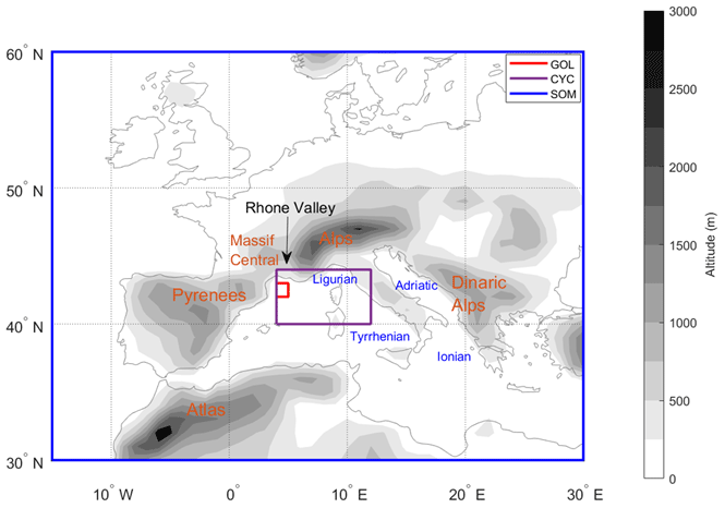
Figure 1 Geographical domains used in the analysis (see Methods section). The whole domain is used as SOM analysis input; the subregion where the Genoa cyclones are detected (CYC) and the subregion in which a northerly flow is required by the mistral definition (GOL) are marked in purple and red boxes, respectively. The topographic height from ERA-Interim is shown in shading (m).

2.1 Data and mistral criteria

The data used to objectively define mistral days was obtained by a combination of the ERA-Interim reanalysis (Dee et al., 2011) of the European Centre for Medium-Range Weather Forecasts (ECMWF) and the regional climate model WRF-ORCHIDEE, downscaled from ERA-Interim, for the years 1981–2016. The WRF-ORCHIDEE model, at 20 km resolution, was performed by the IPSL regional climate model (RegIPSL). The modeling framework is similar to Lebeaupin-Brossier et al. (2013) but uses the land surface model ORCHIDEE instead of DIFF (Drobinski et al., 2012; Guion et al., 2021).

To identify mistral days, first, a Genoa cyclone database is defined based on the presence of a cyclone in the CYC domain (Fig. 1) in ERA-Interim, using the sea-level pressure field at 1^∘ horizontal resolution and 6-hourly time intervals. The cyclone masks are identified in ERA-Interim, at every 6 h time step, as the area within the outermost closed contour around local minima of the sea-level pressure field using 0.5 hPa intervals, adapted from Wernli and Schwierz (2006). To fulfill the cyclone criteria, a day should have at least one time step in which a cyclone is identified. Then, wind direction and speed criteria were applied to days when a Genoa cyclone is detected. This coupling between the wind speed in the GOL and cyclone in the Genoa region is considered the fundamental of lee cyclogenesis in the Alps (Drobinski et al., 2005; Flamant, 2003; Lebeaupin-Brossier et al., 2013; Burlando, 2009) and reassures that the mistral set of events under consideration is analogous to events of lee cyclogenesis, filtering out northerlies stemming from sea-breeze dynamics (Drobinski et al., 2018). The wind criteria are defined as follows, using the daily WRF-ORCHIDEE model data that allow higher spatial resolution: NW to NE (i.e., ±45^∘) wind direction at 900 hPa and 10 m wind speed of at least 2 m/s, averaged in the GOL domain (Fig. 1). The objective identification yielded 2734 mistral days, comprising 21 % year-round frequency, in agreement with Burlando (2009). Consecutive mistral days were grouped into mistral events. The identified mistral event duration and monthly frequency are shown in Fig. 2. Mistral events peak typically in January–February at 30 % frequency, while the mistral is less frequent in summer (∼ 10 %). Most mistral events last a single day. Duration of more than 4–8 d occurs exclusively in the autumn and winter months. This distribution generally agrees with the climatological lifetime properties of the Genoa low (e.g., Campins et al., 2011). The mistral identification method is robust with regard to variations in the wind speed threshold and shows large sensitivity to the allowed wind direction. The additional criterion for the presence of a cyclone constrains the mistral frequency to the range of 20 %–30 %, depending almost entirely on the opening angle criteria.

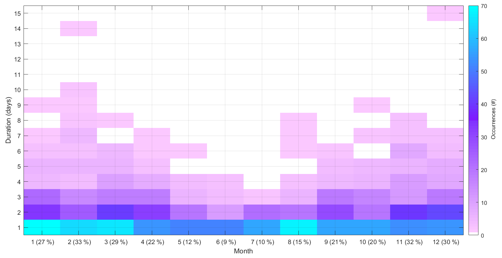
Figure 2 Climatological monthly frequency of mistral duration (days). Shading represents the number of events within the division, for the entire time period. The percentages on the x axis show the monthly frequency of mistral days.

2.2 Isentropic PV classification

2.2.1 Approach

To understand the variability of the synoptic environment during mistral, isentropic PV was classified during all identified mistral days. The classification was achieved by the self-organizing map (SOM) algorithm, reviewed by Sheridan and Lee (2011) and Liu et al. (2011) in the context of synoptic meteorological classification. In contrast to more conservative clustering methods, the SOM encompasses the full continuum of the system's variability rather than only the dominant mean states. According to Sheridan and Lee (2011), for a successful SOM clustering analysis, the variance of the analyzed field is to be well represented by a sequence of consistent system states, each of which corresponds to an objectively related group of samples. The choice of isentropic PV as the input field for the SOM analysis stemmed from both the natural advantages of using a conserved quantity and its wide range of manifestations relevant for the mistral wind. Isentropic PV enables us to depict fine structures such as PV streamers and cutoffs attributed to Rossby wave breaking, compared to the smoother geopotential height field. The main guidelines for a successful clustering analysis were a clear seasonal separation, a large enough number of members for each cluster and a captured PV distribution that will emphasize the fine structures that are often averaged out of long-term PV composites. Huang et al. (2017) used a SOM algorithm combined with hierarchical ascendant classification (HAC) (Jain and Dubes, 1988) to classify winter 300 K isentropic PV regimes over eastern Asia and related the classes to cold surges occurring in eastern Asia. Here, the data used for the clustering analysis are the ERA-Interim daily mean vertically averaged upper-tropospheric isentropic PV field, within the SOM domain defined by the blue box in Fig. 1. Isentropic PV is averaged between the 320–340 K isentropic levels, with intervals of 5 K. This averaging is meant to overcome the seasonal temperature variation and allow a year-round analysis (Wernli and Sprenger, 2007). As the SOM algorithm is optimized for input values ranging from 0 to 1, the vertically averaged isentropic PV distribution is rescaled by the ratio between the mean PV and the mean standard deviation, specifically

$$\begin{array}{}\text{(1)}& {\mathrm{PV}}_{\mathrm{norm}}={\mathrm{PV}}_{(x,y,t)}\cdot \left({\displaystyle \frac{\stackrel{\mathrm{‾}}{\mathrm{PV}}}{\stackrel{\mathrm{‾}}{\mathrm{SD}}}}\right),\end{array}$$

where the overbar denotes spatiotemporal average; thus the ratio on the right-hand side is a constant equal to 0.0732, so that PV_norm is roughly distributed between 0 and 1, as required by the SOM algorithm. Here, the SOM analysis is performed for the domain between 30–60^∘ N and −15–30^∘ E – a compromise between the largest domain centered at the GOL that preserved a seasonal signal and the preservation of the identified flow patterns captured by its smaller alternatives.

The SOM attributes each mistral day to one cluster. Using ERA-Interim data, we further examined the mean surface conditions for each of the resulting clusters of mistral days to unravel the possible link between the different PV-based clusters and the surface flow, surface turbulent heat fluxes, temperature and precipitation. Transitions among clusters during the mistral wind were then systematically examined to reveal recurring transition sequences and their seasonal variability. Finally, we demonstrate the representativeness of the clusters and transition paths to individual cases.

2.2.2 SOM setup and validation

The SOM algorithm is provided by MathWorks (https://www.mathworks.com/help/deeplearning/gs/cluster-data-with-a-self-organizing-map.html, last access: 15 July 2021). The setting used in the present study yielded a shallow neural network with a single layer, using the sigmoid activation function, in a hexagonal grid (Fig. A1). The hexagonal grid setting implies that each cluster interacts with the six surrounding clusters in terms of similarity; however, the results are displayed on a rectangular grid to simplify the presentation. The choice of the map dimension (and therefore number of clusters) was set as the number beyond which the classification method begins to deteriorate or does not add relevant information (i.e., near empty clusters or highly similar ones). Here we aimed to classify the mistral events into clusters that pose dynamically meaningful PV distributions, representative of their daily individual members, and with a considerable annual mean frequency (i.e., on the order of 5 %). Eventually, the number of clusters was set to 16 in a 4×4 configuration (Fig. A1), which satisfied these demands.

The SOM algorithm learning process optimizes a chosen function indicating each cluster's inner variance, and despite the wide variety of relevant functions, well-performed SOM processes are usually quite indifferent to the chosen function (Sheridan and Lee, 2011). This statement is usually true for other chosen parameters such as the neighborhood size and calculation time steps, within a reasonable range of values (e.g., Cassano et al., 2006; Johnson et al., 2008). For the present study we chose the intuitive mean squared error (MSE) function as the optimization parameter with the initial neighborhood distance set to 2 and number of training steps for initial covering of the input space set to 365. Indeed, the identified patterns were only weakly affected by the choice of these parameters. Furthermore, the SOM readily reproduced similar average patterns for several different mistral datasets. For example, the process was repeated for a subset of mistral dates in which single-day mistral events were removed and events separated by a single day were joined. This modified subset included 248 d less than the original, reducing the sample size by over 10 %, yet the identified patterns were nearly identical.

Statistical significance is assessed by a Student t test between each cluster and the total averaged mistral flow. Following Wilks et al. (2016), an additional criterion was added to the statistical test to account for the multiple testing problem. Specifically, the Walker criterion was applied, where a threshold of ${\mathit{\alpha }}_{\mathrm{walker}}=\mathrm{1}-(\mathrm{1}-{\mathit{\alpha }}_{\mathrm{0}}{)}^{N_{\mathrm{0}}^{-\mathrm{1}}}$ is set on the p value obtained by the t test. α₀ is the required significance level (e.g., 0.05 for 95 % confidence) and N₀ the number of individual t tests or, in this case, the number of grid points in the domain of interest. If the p value of an individual t test is larger than α_walker, the null hypothesis cannot be rejected at a level of α₀.

3 Results and discussion

3.1 PV distribution clusters

The classification of isentropic PV resulted in 16 clusters, set in a 4×4 hexagonal grid, where similar clusters are placed closer together in the SOM space. The identified mean PV patterns defining each cluster are displayed in Fig. 3, alongside the mean 500 hPa geopotential heights. The panel order represents each cluster location in the SOM space; i.e., the least similar clusters are placed farther apart in the SOM space, and more similar ones are placed adjacent to one another. Some clusters correspond to exotic upper-tropospheric PV structures, such as thin streamers and cutoffs, attributed to different Rossby-wave-breaking (RWB) events. Dotted regions indicate statistical significance, i.e., the main features by which the classification process is established. For instance, a high PV tongue to the west of a cutoff appears to define cluster 8, while a westward stretching PV streamer defines cluster 9, suggesting these clusters correspond to cyclonic and anticyclonic RWB life cycles (Thorncroft et al., 1993), respectively. A southwesterly oriented cutoff defines cluster 5, while a northerly thin streamer defines cluster 2, and so on. Together, the clusters illustrate a thematic separation of the PV continuum responsible for mistral events, and one can easily envision how the waves propagate by switching from one cluster to another.

Upstream of the high-PV anomaly, most clusters exhibit an amplified ridge in the upper troposphere over the Atlantic, a common precursor for intense Mediterranean cyclones (Raveh-Rubin and Flaounas, 2017). As expected, the primary mode of variance is in the seasonal cycle, manifested by the meridional shift of the dynamical tropopause (Sect. 3.2). Another mode apparently picked up by the SOM is evident when comparing clusters 12 and 16 to 11 and 15. Evidently, the SOM was able to distinguish between mountain-passed PV anomalies (11 and 15) and blocked ones (12 and 16), and the impact on the trough properties is evident by the tilting of the trough axis upon the passage across the Alps from NE to N, respectively. The standard deviation (SD) for the PV distribution within the clusters is presented in Fig. A2 in the Appendix, emphasizing the different active regions between the clusters.

Note that the composites presented on Fig. 3 each constitute ∼ 100 d. While some variance within the clusters is inevitable, these composites help to illustrate the SOM clustering process, especially in statistically significant regions. Detailed features of the actual patterns, as picked up by the SOM, can be better understood by carefully examining the cluster members with respect to their mean values. Such examples are provided in Sect. 3.6, aiding in establishing the cluster features, detailed in Table 1.

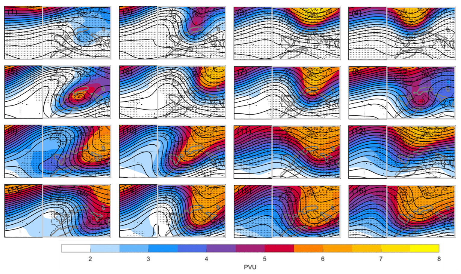
Figure 3 Daily mean vertically averaged isentropic (320–340 K) PV (PVU, color) and 500 hPa geopotential height (unlabeled black contours, 30 m intervals) of the SOM-identified clusters. The topographic height contour of 700 m is shown in dark grey. Dotted regions indicate statistical significance > 95 % for the PV composites compared to the average mistral flow. The bright grey frame indicates the domain in which the SOM classification was done.

3.2 Seasonal variation

The climatological monthly occurrence frequency of each cluster is displayed in Fig. 4, demonstrating the strong seasonal affiliation of the clusters; i.e., all clusters have a clear seasonal peak in their occurrence. Clusters 1–4 occur mostly between June and October, while clusters 9–16 occur mainly between November and April. The low-PV background clearly dominates summer clusters (Fig. 3 panels 1–4), while much broader wave amplitudes constitute the winter clusters (9–16). In between, clusters 5–8 peak mainly in the transition seasons. Overall higher frequencies are obtained in the winter clusters, as expected by the larger frequency of mistral events appearing in winter.

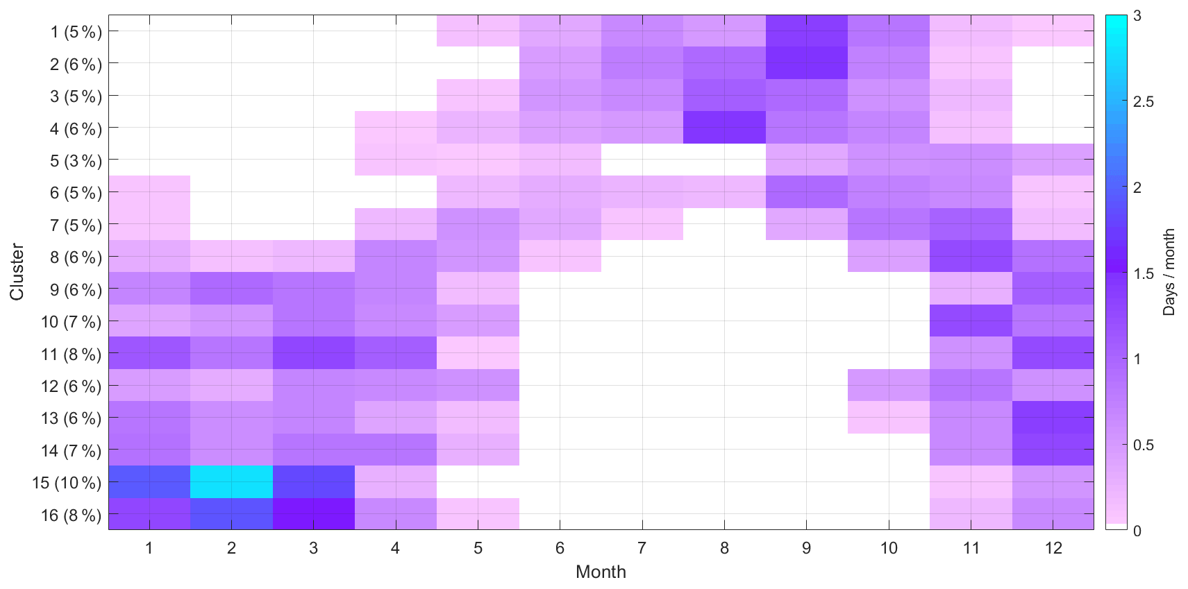
Figure 4 Monthly frequency of the classified mistral clusters (days per month). The percentage of mistral days corresponding to each cluster is shown on the y axis (%).

3.3 Surface circulation and surface impact

The surface impact of the differently classified mistral events is presented in terms of composites of sea-level pressure (SLP) and precipitation (Fig. 5) and surface heat fluxes (SHFs) along with 10 m winds and 900 hPa equivalent potential temperature (Fig. 6).

The SLP patterns reveal the typical westward tilt with height and suggest that some clusters favor a phase lock, usually corresponding to the deepest cyclones (e.g., clusters 5, 8 and 14–16). It is probable that each PV cluster is linked to a different stage of the cyclone life cycle, which can be centered to the east or west of Italy, or even south in the Ionian Sea, with varying depths. The cyclones are closest to the lee of the Alps in clusters 4, 8, 12 and 16, associating the right column in Fig. 3 to the initial stages of cyclogenesis, while the left column (clusters 1, 5, 9 and 13) likely correspond to the termination stage of the cyclones and their easternmost location. The anticyclone extending from the Atlantic is highly variable among the clusters in its strength, thereby affecting the surface pressure gradient, and its spatial extension towards Europe. At times, the high-pressure system dominates the region (e.g., clusters 1, 6, 9 and 13), such that a weak cyclone is sufficient for producing the strong mistral winds (see red arrows in Fig. 6). In other cases, the deep Mediterranean cyclone is the dominant feature (e.g., clusters 11, 12, 15 and 16).

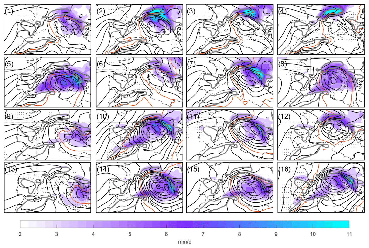
Figure 5 The same as Fig. 3 but for a smaller domain showing SLP (hPa, black contours) at 1 hPa intervals below 1015 hPa (colored line) and 2 hPa intervals above 1015 hPa. Daily accumulated precipitation (mm/d) is shaded. Dotted regions indicate statistical significance > 95 % for the precipitation composites compared to the average mistral flow.

The mean distribution of precipitation is unique for every cluster, with the location of the precipitation maxima differing among clusters more than across the seasons. In summer, precipitation varies sharply between the eastern and northern Alps (i.e., clusters 1–4), while in the winter it is differently distributed between the Dolomite and Balkan Mountains, (i.e., clusters 12 and 16) and the Alps (8), with notable precipitation occurring along the African shoreline as well (10, 14, 15 and more). Generally, precipitation is distributed along the northern and eastern sides of the cyclone and roughly correlates with its intensity, which is consistent with previous work (Flaounas et al., 2015; Raveh-Rubin and Wernli, 2015, 2016).

The surface heat flux pattern associated with each cluster is relatively localized. Most clusters exhibit the familiar heat loss hotspot in the GOL; however, it can extend to different lengths south into the Mediterranean and is absent from several clusters (specifically, 8, 9, 12 and 13). The bora winds are active together with the mistral when upper conditions allow for an easterly flow towards the Adriatic Sea in central-eastern Europe (i.e., clusters 5, 9, 13 and 14), generating heat loss hotspots in the Adriatic.

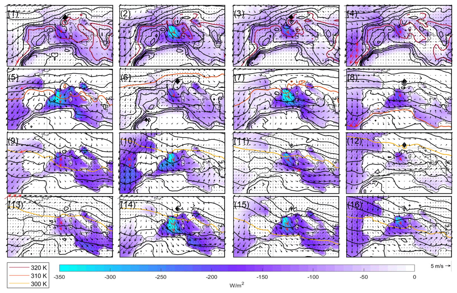
Figure 6 The same as Fig. 5 but for surface heat fluxes (sum of sensible and latent, W/m²) in color; equivalent potential temperature at the 900 hPa level in black contours at 2 K intervals; and the 300, 310 and 320 K isotherms in color (see legend). Black arrows denote 10 m wind vectors, where red arrows mark winds above the local 75th percentile. Dotted regions indicate statistical significance > 95 % for the surface heat flux composites compared to the average mistral flow.

The direction and horizontal extent of the mistral wind also differs between the clusters, with clusters 2, 7, 14 and 15 apparently delivering the strongest winds that also extend the furthest into the Mediterranean. The equivalent temperature field illustrates the cold and dry anomalies caused by the mistral. Differences are evident between the clusters, with some displaying a frontal deformation of the isotherms around the Gulf of Genoa. Interestingly, clusters without a marked cold/dry anomaly correspond to clusters with only weak fluxes, despite the strong surface winds (clusters 8, 9 and 13).

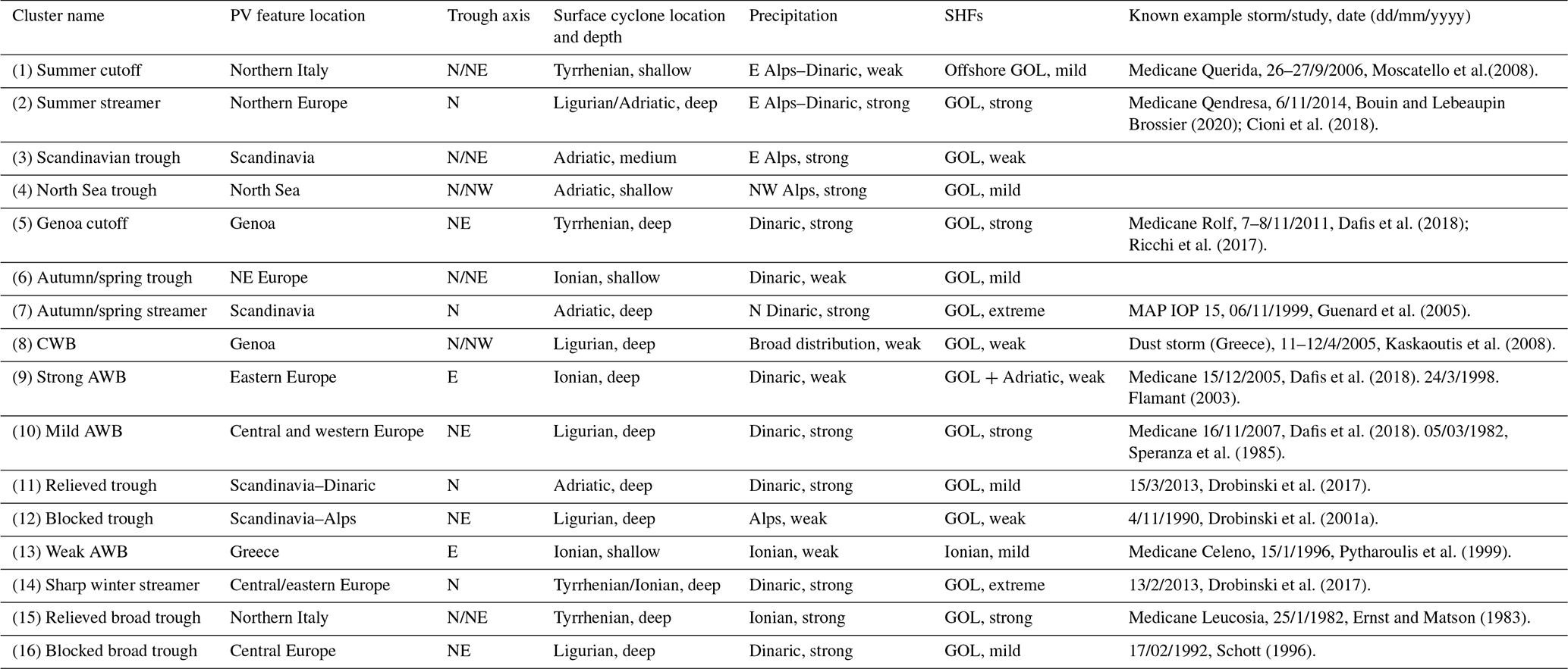
Note that the statistical significance presented in Figs. 3, 5 and 6 is compared to the average mistral flow, thus highlighting the changes between the different mistral clusters, rather than deviations from climatology. For example, referring to Fig. 6, the SHF maxima in the GOL are often not statistically significant as they are a standard mistral feature (clusters 6, 11 and 16). However, statistical significance arises when the signal extends further south (clusters 2, 7 and 14), when it extends further west (clusters 5 and 10) or if it is exceptionally weak (clusters 1, 12 and 13). The clusters' main characteristics are summarized in Table 1, along with the attribution of known mistral cases and/or Mediterranean cyclones to the PV-based clusters.

Table 1 Summary of cluster names and main features. AWB/CWB refer to anticyclonic/cyclonic Rossby wave breaking, respectively.

3.4 Time evolution of mistral events

Frequent cluster transitions and cluster persistence can be visualized using the transition probability matrix (TPM, Fig. 7). Column 0 shows the likelihood of a mistral event to end at any cluster with no further transition. The strong amplitude along the shifted main diagonal suggests that every cluster has a tendency to sustain itself, at a varying likelihood. We interpret this feature as a persistence demonstration by the algorithm, as the timescale for the evolution and migration of the PV structures driving the mistral events is often longer than a day. The fact that the PV-based SOM is able to consistently classify consequent events of slow-developing waves under the same classification reinforces the robustness of the method, given proper SOM constraints (such as the number of clusters), as only significant (by SOM interpretation) differences in the daily fields within a mistral event can force a transition. After Espinoza et al. (2012), a transition is deemed statistically significant if its frequency exceeds the 90th percentile of the corresponding transition frequency derived from a 1000 random redistributions of the original sequence. We constructed a reference random distribution by considering all mistral days (recall that the clustering is performed only for mistral days and not for all other days). While Huang et al. (2017) set their criteria using the 95th percentile, here the 90th percentile threshold was selected, considering that single-day mistral events represent roughly 50 % of mistral events and are of less interest from the dynamical perspective. Nevertheless, post-mistral days are accounted for as eligible transitions in the random distributions, represented by the 0 column in Fig. 7.

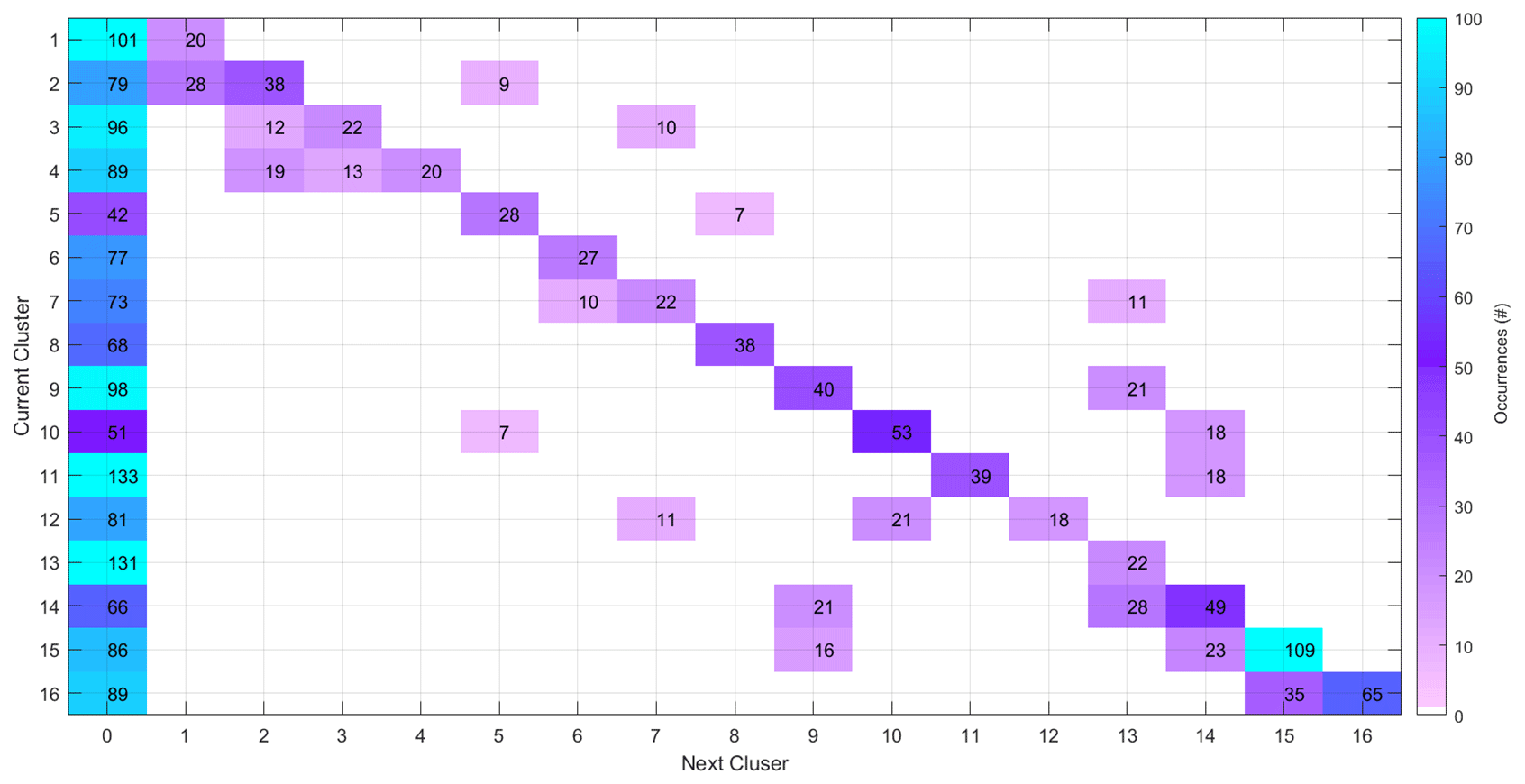
Figure 7 Transition probability matrix, based upon daily cluster transitions from the current cluster to the cluster on the next day (colored by number of days). The total days in each transition are given by the numbers in the corresponding rectangle. The 0 column represents the ending of mistral events, and the diagonal represents the probability to remain in the same cluster for the next day. Only statistically significant (90 % confidence level) transitions occurring within mistral events are shown.

Note that the transitions are distributed mostly around the main diagonal and the 0 column; the latter is primarily due to frequent single-day mistral events. Nonetheless, some recurring cluster transitions are showing a considerable amplitude, such as transitions 14 → 9 and 2 → 5 and others. These transitions are made clearer when viewed separately for each season (Fig. 8). Very different amplitudes along the main diagonal and the 0 column suggest some clusters are only self-sustaining in certain seasons and are more likely to be the end of a mistral event in the other seasons (for example, cluster 5 in autumn compared to winter–spring). It is clear from the seasonal TPMs that some transitions are absent from certain seasons, whereas others may occur at any month of the year. Studied carefully, these transitions reveal many details about the development of upper-level PV anomalies over the Alps. For instance, transition 12 → 7 (amplifying ridge behind streamer) and 10 → 5 (formation of Genoa cutoff) are more abundant in the transition seasons, while transition 14 → 9 (strong anticyclonic Rossby wave breaking, AWB) occurs in any season except the summer, suggesting this transition and several others are more resilient to the changes of the seasons. Some of these transitions, and indeed some individual clusters, can be directly related to AWB (14, 15 leading to 9, and 13), cyclonic Rossby wave breaking (CWB, cluster 8), a cutoff low migrating into the domain from the north (2 → $\mathrm{1}/\mathrm{5}$), or being cut out of a northeasterly streamer (10 → 5). Other transitions imply an equatorward stretching of a trough (12 → 10), or the eastward propagation of a trough (4 → 3, 7 → 6), and so on. These features shed light on recurring wave-evolution processes and allow one to easily access and investigate a large variety of rare yet dynamically similar events by selecting certain cluster transitions that are representative of certain wave life cycles.

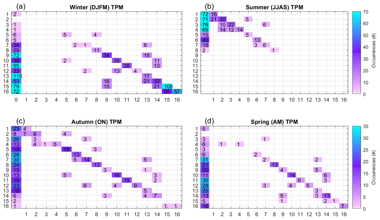
Figure 8 The same as Fig. 7 but separating by the different seasons. Note the 2-month periods in autumn (October–November) and spring (April–May), compared to 4 months in winter (December–March) and summer (June–September), and the different color scales, accordingly.

Considering that many mistral events last more than a couple of days, it is insightful to examine the first event transitions rather than all individual transitions without a time trace (as in Figs. 7 and 8). Therefore, we first identify the mistral initiation days, with respect to each cluster, and then display the first two transitions for every mistral event in the group. Despite containing tens of individual transition sequences at each mistral group, several dominating first transition sequences emerge (i.e., same sequence of days 1–3). Recurring transitions exhibit a strong seasonal dependency (Fig. 9). Qualitatively, the transition sequences seem to “push” the system towards seasonally dependent preferable clusters. Thus, an event initiating with an off-season cluster, say cluster 6 in winter, will be shifted towards the proper winter cluster 13, suggesting the broadening of the northerly streamer into a mature trough. Another example can be seen in the initial clusters 4 and 8, where the first transitions are seasonally dependent. In wintertime, mistral events are dominated by the transitions between clusters 9–11 and 14–16, with preferable paths illustrated by the thick blue lines in the corresponding panels. This view also highlights the directionality of the transitions. For instance, note that the clusters with the largest numbers of initiated events that last 3 or more days are the blocked clusters 12 and 16 and that the “relieved” clusters rarely jump back to a blocked cluster; i.e., the transitions $\mathrm{11}/\mathrm{15}$ → 12 are scarce. Considering the cluster configuration displayed in Fig. 3, the general direction of flow within a mistral event is from right to left and from top to bottom, diverging mostly from clusters 8 and 12 and converging towards clusters 9, 14 and 15 (see Fig. S1 in the Supplement).

Figure 9 Transition sequences (days 1–3) for mistral events initiating with each cluster at mistral day 1 and lasting at least 3 d, at every season (using the same 2- and 4-month seasonal definitions as in Fig. 8). The x axis represents days passed from mistral initiation. Solid lines indicate transition sequences (days 1–3) that repeat 2–4 times throughout the time period. Thick lines emphasize sequences occurring 5–10 times, while dashed lines denote single-occurrence sequences.

Overall, the clustering analysis identified robust and distinct isentropic PV patterns, and the transition analysis offers additional perspective on the evolution of these upper-level PV structures as they interact with the Alpine ridges during mistral events. These TPMs, combined with the surface impact of each identified PV cluster, can potentially be utilized to improve weather predictions of both the mistral wind and the Genoa cyclone, as well as their impacts. In the following we examine three individual mistral events and the ability of the cluster mean to represent their evolution in a meaningful way.

3.5 Three illustrative mistral events

The qualitative view of the algorithm performance is presented by a comparison between the classified clusters and the individual members for three mistral events. The large-scale structure of the PV is, however, well captured by the SOM, as illustrated in the following cases.

3.5.1 Anticyclonic wave-breaking mistral, 16–20 January 1987

This winter mistral event initiated with a broad, mountain-passed winter trough that engulfed most of continental Europe. Strong surface heat fluxes commenced on day 1 as the trough stretched over the Alps into day 2, with the transition 15 → 14, accompanied by a deepening of the cyclone, and intensified precipitation and GOL heat flux, as implied by the intense mistral events generally classified in cluster 14. Another transition back to 15, from day 2 to 3, implies another broadening of the trough, with a slight weakening of the mistral and persistence in cluster 15, a common scenario (Figs. 8 and 9). The wave is then deflected to the east of the Alps and breaks anticyclonically, as captured by the transition 15 → 9. On its last day at cluster 9, the cyclone is weakened, along with reduced associated surface heat flux and precipitation, as is indeed common for cluster 9.

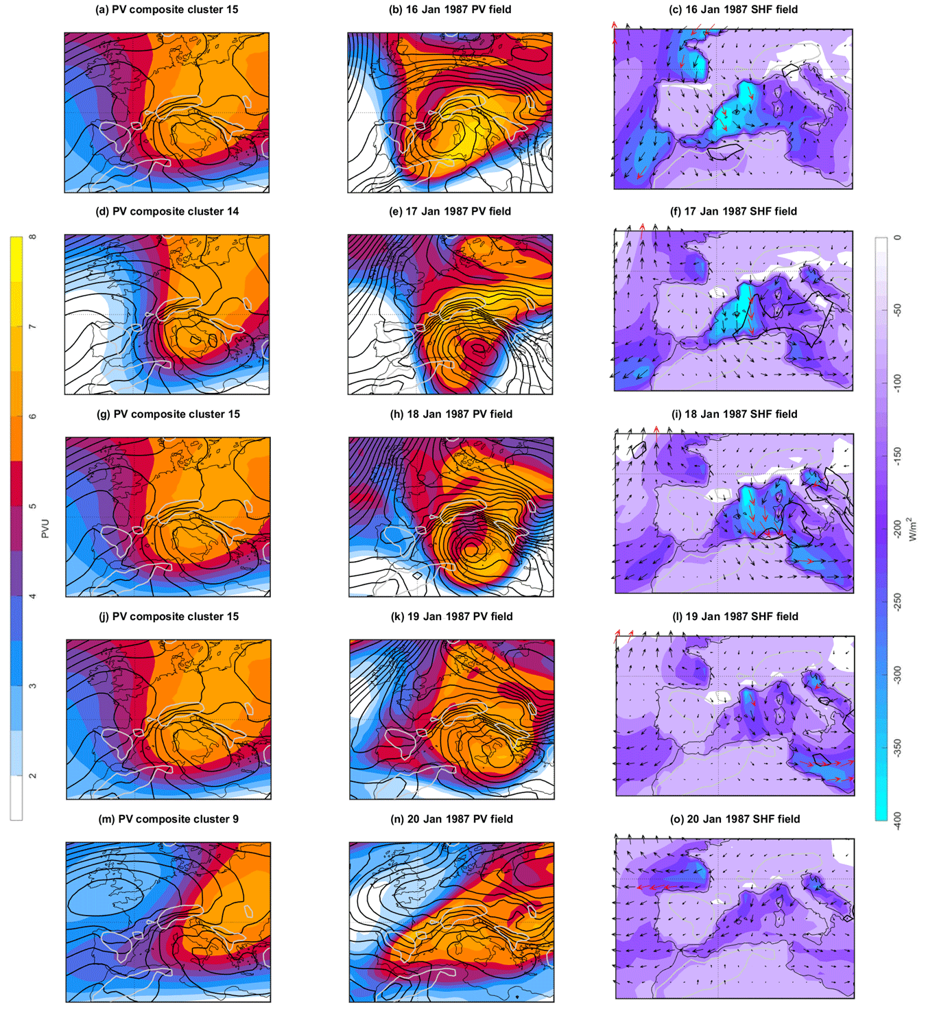
Figure 10 An illustrative AWB event identified by the transition 15 → 9. Shown are vertically averaged (320–340 K) daily PV distributions and SLP (black contours) throughout a mistral event (middle column), alongside their corresponding cluster composites (left column). Surface impact is shown on the right column in terms of the sum of sensible and latent heat fluxes (W/m², shaded), 10 m wind vectors (the red vectors represent magnitude in the upper quartile) and daily accumulated precipitation (black contours, 10 and 30 mm/d).

3.5.2 Cyclonic wave-breaking mistral, 8–12 April 2005

This spring mistral event begins with a blocked trough and a weak cyclone in the lee of the Alps. The trough is stretched into a thin NE streamer, captured by transition 12 → 10, representing a common transition. Upon this transition, which marks a first AWB, the SHFs intensify dramatically, along with precipitation in the Adriatic region. The trough then further stretches and breaks cyclonically (10 → 8) to form a cutoff, as the cyclone attains a deep symmetric structure (Tous and Romero, 2013). Note that the streamer is channeled above the Rhône valley just before breaking, illustrating the wrapping up of PV banners generated in the mistral region (Aebischer and Schär, 1998). The classification of 11 April 2005 to cluster 8, capturing the CWB pattern despite the PV streamer extending to the northeast rather than northwest as suggested by the composite, emphasizes the ability of the SOM to identify distinct geometrical features rather than only geographical ones.

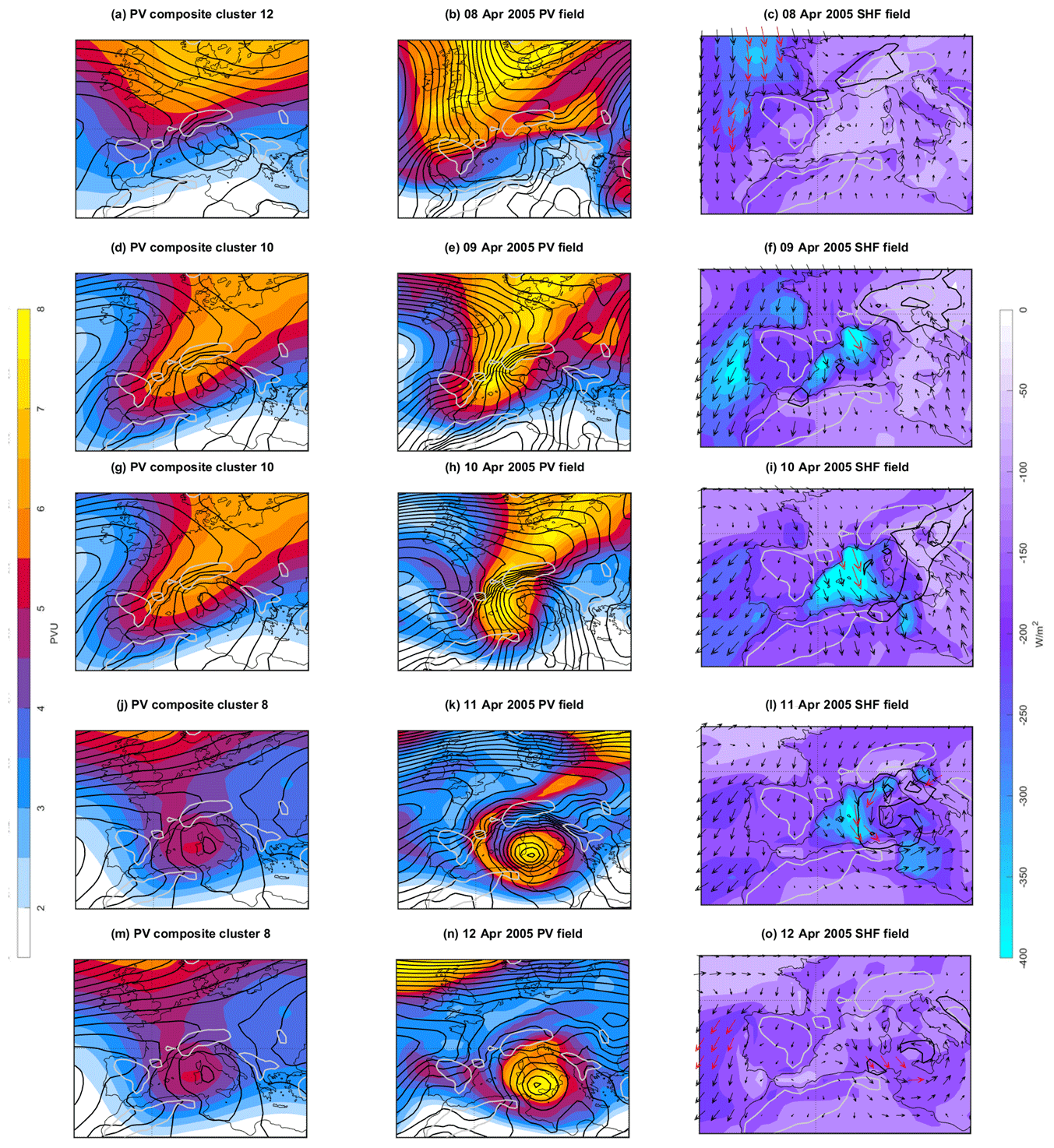
Figure 11 As in Fig. 10 but for a CWB event identified by the transition 10 → 8.

3.5.3 Cutoff low mistral, 25–31 August 1995

The summer mistral event is exceptionally long for the season. It begins with the weakest upper-level forcing recorded by the present analysis, with a 2 → 1 transition, demonstrating the cutoff of a 3 PVU northerly streamer over the Alps. The propagation of a second wave into the domain is identified as transition 1 → 3, and this second wave is again stretched southward to form a summer streamer (3 → 2). This transition is accompanied by an intensification of the mistral, the deepening of a primary cyclone southeast of the Baltic Sea and a lee cyclone in the Adriatic Sea. The streamer then tilts and breaks to form a cutoff low (2 → 5), with weakening of the mistral intensity. A noticeable characteristic is the persistent precipitation response of the days corresponding to cluster 2, centered just between the eastern Alps and northern Dolomites, as suggested by the precipitation composites (Fig. 5, cluster 2).

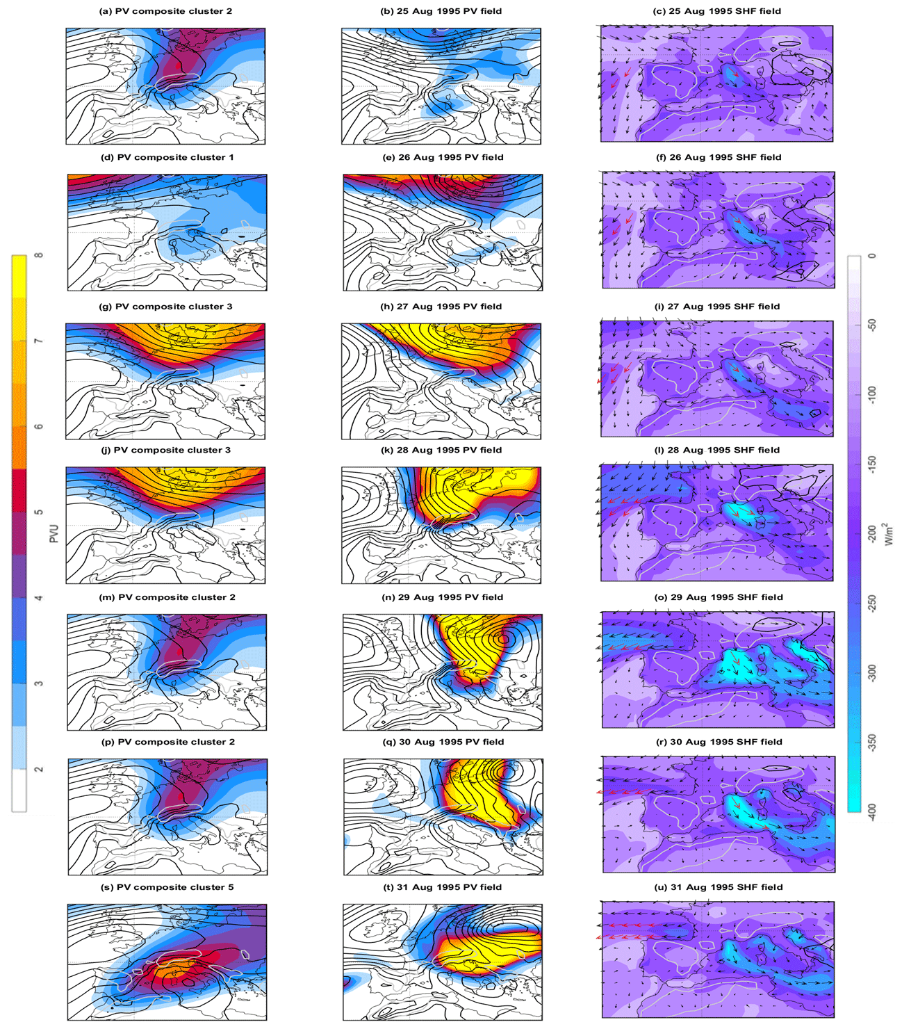
Figure 12 As in Fig. 10 but for a summer cutoff formation event identified by the transitions 2 → 1 and 2 → 5.

4 Summary and concluding remarks

This study examines systematically the large- and synoptic-scale drivers of the mistral wind during 1981–2016 by classifying the isentropic PV during mistrals. Mistral days are first identified objectively in a climatological dataset based on 20 km resolution WRF-ORCHIDEE simulation forced by ERA-Interim, yielding 2734 mistral days distributed among 1360 mistral events. The mistral occurs throughout the year but occurs more often in winter, with more multi-day events, compared to summer. A SOM clustering analysis then classified the PV distributions during mistral days, providing insight on the large-scale driving mechanisms of the mistral wind, and further served as a tool to examine different types of surface impact signatures. Referring to the questions posed in the introduction, here we summarize the main findings (see also Table 1).

• i.

  During objectively identified mistral days, the daily mean, vertically averaged (320–340 K) isentropic PV distributions are classified into 16 distinct clusters according to their geometrical shapes. The emerging features vary among amplified Rossby wave patterns ahead of an Atlantic ridge. Features include troughs, PV streamers with variable orientations indicative of cyclonic or anticyclonic Rossby wave breaking CWB/AWB, and cutoff lows.

• ii.

  The clustering approach distinguishes between the seasons, including the transition seasons, suggesting that a limited range of PV features prevail in each season. In summer, clusters 1–4 suggest the dominance of either a cutoff, thin streamer, or a trough over Scandinavia or the North Sea. In the extended winter season, several AWB scenarios prevail, as well as broad, deep, southward-intruding troughs. In the transition seasons, troughs, streamers cutoff lows and CWB are the dominant features. Note that PV features (e.g., streamer or cutoff low) exhibit different mean position, shape and magnitude across different seasons (see Table 1 for a detailed summary).

• iii.

  Each cluster indeed reveals a unique signature in terms of surface weather impact, i.e., surface cyclone and associated circulation, winds, sensible and latent heat fluxes, and precipitation. The bora wind regime, for example, appears to co-occur with the mistral within clusters 9 and 13, which is expected from a relatively eastern PV anomaly. The latent and sensible heat loss hotspots centered over the GOL strongly vary among the clusters, as does the wind speed and the extension of the mistral wind offshore. The highly variable mean intensity, size and location of the cyclones associated with the different clusters clearly demonstrate the impact of the upper-tropospheric PV distribution on the surface pressure, with most cyclones under a phase lock with a parent trough, implying the lee cyclogenesis effect. The deepest cyclones and strongest surface heat fluxes occur with PV streamers indicative of AWB/CWB, a Genoa cutoff or a deep winter trough. The mean precipitation response strongly depends on the cluster and season, generally being correlated to the mean cyclone intensity and peaking to the north and northeast of the cyclone. At times, precipitation occurs also downstream of the mistral outflow along the north African coast, particularly in clusters with strong surface fluxes. The latter is consistent with Rainaud et al. (2016) and Berthou et al. (2018), who demonstrate the remoistening of the dry mistral air mass and its downstream precipitation impact.

• iv.

  The evolution of the flow types during multi-day mistral events is examined through the analysis of transitions among clusters, while searching for recurring patterns. The dominant direction of transitions corresponds to the eastward drift of the waves (7 → 6, 16 → 15), while other transitions imply the stretching of the PV feature as it approaches the Alps (3 → $\mathrm{2}/\mathrm{7}$, 12 → 10) or the formation of a cutoff (10 → 5). Long mistral events (> 2 d) initiate mostly with the blocked clusters 12, 16, and 10 and tend to end with AWB/CWB events, i.e., cluster 8, 9, and 13, or with a cutoff (clusters 1, 5). The prior is mainly evident by the non-uniform distribution of the mistral initiation days between clusters (Fig. 9) and the latter by the lack of transitions from these clusters (1, 5, 8, 9 and 13) to other ones. Specifically, clusters 1, 8 and 13 do not transit to any other cluster (within the 90 % confidence level; see Fig. 7), with clusters 5 and 9 only transiting to 8 and 13, respectively. Cluster 14 represents the strongest mistral events in terms of heat fluxes and wind speeds, while clusters 12 and 13 correspond to the weakest. Cluster 15 is the most persistent and abundant, whereas cluster 12 is the most transient.

The SOM performance is evaluated quantitatively by standard deviations within the cluster (Fig. A2) and qualitatively by comparing individual members to their corresponding cluster composites. It is evident that even highly non-linear Rossby-wave-breaking processes are well represented by their corresponding cluster composite means, while the inevitable case-to-case variability is manifested mainly along the high PV gradients, or in terms of the magnitude or location of the PV anomaly of cutoffs.

One primary conclusion implied by the present classification arises when attempting to examine the present clusters under the cyclone types as defined by Buzzi and Tibaldi (1978). According to the classic description of lee cyclogenesis, the initial phase of the lee cyclone is attributed mostly to a geostrophic adjustment process, induced by the mountain, generating the cyclone rapid deepening rates in a still relatively barotropic environment. In the latter phase, thermal gradients are enhanced due to the advective nature of the Rossby wave, and baroclinic instability becomes the dominant mechanism influencing the cyclone, as the low-level cold-pool air mass finally flows across the topography. Carefully examined, some clusters can be related to phase 1 or 2 of the lee cyclone, according to their representative thermal gradients, and PV maxima location relative to the Alps. The so-called “blocked” modes, i.e., 12 and 16, appear to correspond to a much weaker mistral event in terms of wind speeds and GOL surface heat fluxes, when compared to their “relieved” companions, 11 and 15. This suggests that the maximum mistral-related surface heat fluxes are attributed to the baroclinic phase of the cyclone rather than the triggering phase. While further confirmation of this perspective is required, it settles with the notion of the mistral as “one of many strong winds that manifest the penetration of cold air into the Mediterranean from the north” (Scorer et al., 1952), in the sense that a strong mistral indeed enables a significant penetration of polar air masses into the Mediterranean, leading to the massive heat loss at the GOL occurring at post-blocked stages of the mistral event rather than in the initial stages.

This aspect of the mistral and Genoa cyclogenesis as a synoptically controlled phenomenon has the potential to improve predictions of the mistral wind and Genoa cyclogenesis events and deepen the understanding of synoptic-scale PV interactions with topography. Furthermore, the systematic classification offers new insight into the variability of the mistral impact on air–sea interaction in the region, with direct implications for understanding the seasonal buildup and onset of deep convection in the water column in autumn–winter.

Appendix A: The 4×4 hexagonal SOM map

The SOM neighbor distance is a measure of similarity between neighboring SOM clusters, specifically the mean squared error (MSE) between the SOM weights corresponding to the neuron that represents each cluster. The 4×4 hexagonal SOM map and the neighbor distances are presented in Fig. A1. The smaller the neighbor distance the more similar the neighboring clusters. This measure does not involve the frequency of transitions between clusters, discussed in Sect. 3.4. The similarity map exhibits a dark line of reduced similarity crossing the grid, defining the seasonal separation discussed in Sect. 3.2. With that said, there is a physical reason for similar clusters to appear consecutively, and a transition between two very different clusters, e.g., 8 → 3, would seem very unlikely. Thus, the transition-season clusters are expected to provide a corridor through which summer clusters can develop into winter clusters, or vice versa (especially cluster 7).

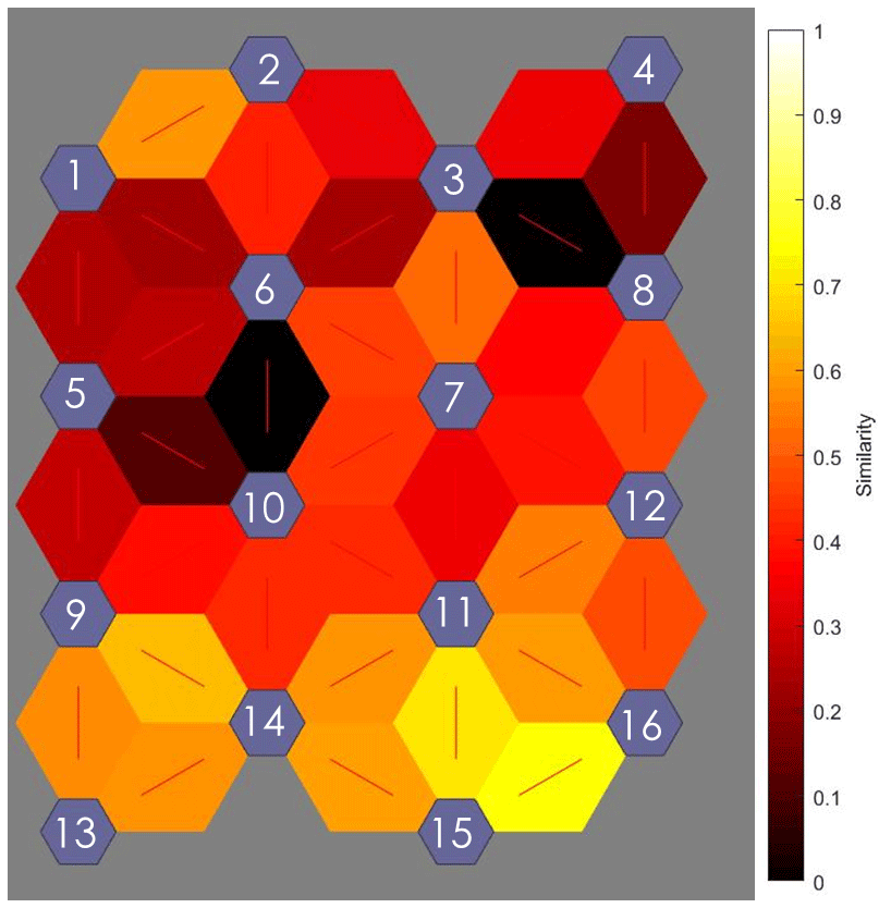
Figure A1 The 4×4 hexagonal SOM map with the numbered clusters and neighbor distances, or similarity between clusters (dimensionless) in colored connections. Brighter colors represent short distances, or more similar clusters, and dark colors indicate long distances, or dissimilarities.

Appendix B: Intra-cluster variability

The variability among the members for each cluster can be quantified with the standard deviation (SD) map of the PV fields (Fig. A2). The resulting patterns demonstrate the uncertainty in the magnitude and exact location of the identified PV feature. As such, the largest SD is either along the boundary of the streamer (e.g., clusters 3, 6, 10 and 14) or within a cutoff (1, 5 and 8). It is apparent that some clusters mean signal is reasonably well aligned with the individual members, while others exhibit larger inner variance. For example, most members of cluster 9 fit right in the composite, as opposed to cluster 1, where the cutoff magnitude is likely underestimated by the averaged field, due to variations in location. The SD also reveals further details on some clusters, such as the hidden PV streamers apparently related to clusters 6 (towards the Atlas Mountains) and 3 (towards the Pyrenees). The mean SD for most clusters is on the order of 15 %; however, the major correspondence between the composite and its members is along the maximum PV gradient bands, and the quantitative inaccuracy is compensated for by the qualitative description of the flow (i.e., Figs. 10–12). Compared against the 95 % statistical significance (Fig. 3), focusing on cluster 5, the low-SD region in the middle of the cutoff is translated into statistically significant signal, while its surrounding peak in SD is translated into non-significant regions, again demonstrating the variability regarding the extent of the identified cutoff. Similar links between the SD and statistical significance are evident in clusters 2, 7 and more. Quantization and topographical errors (QE and TE, respectively) are evaluated after Kiviluoto (1996) and are presented per cluster and averaged for the entire network in Fig. A2. QE is the average distance (in terms of the SOM optimization function, in this case MSE) between samples and their corresponding cluster. TE measures the continuity of the SOM space by evaluating the proximity of the first and second most important clusters, for each input sample. Ideally, both QE and TE should be minimal. While QE generally behaves similarly to the standard deviation within the clusters, large TEs usually imply a folding of the SOM space due to a hidden dimension of variability. This dimension of variability generates distant yet similar clusters, as it is secondary to the main dimensions that make up the SOM space. The algorithm then attempts to reduce the distance along this extra dimension by folding the SOM space. In the present case, this hidden dimension appears to correspond to the discontinuity and deformation of the PV feature, i.e., the extent of separation between the PV streamer and its parent reservoir and the amount of stretching of the PV streamer. This dimension of variability is secondary to both the meridional and zonal dimensions of variability. Thus, the largest TE is attributed to the cutoff clusters 5 and 8, suggesting a fold of the SOM space bridging the apparent distance between the two objectively similar clusters. The heavily deformed cluster 10 exhibits a considerably large TE, possibly also due to the mentioned fold in the SOM-space.

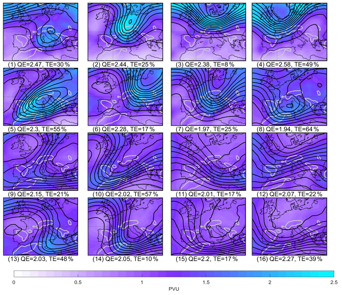
Figure B1 Standard deviation (SD) of isentropic PV within each cluster. The quantization and topographic errors (QE in PVU and TE in %, respectively) are noted at the bottom of each panel, following the cluster number. The average QE and TE for the network are 2.2 PVU and 30 %, respectively.