the Creative Commons Attribution 4.0 License.
the Creative Commons Attribution 4.0 License.
 | 23 Jul 2021
On the occurrence of strong vertical wind shear in the tropopause region: a 10-year ERA5 northern hemispheric study
Daniel Kunkel
Peter Hoor
A climatology of the occurrence of strong wind shear in the upper troposphere–lower stratosphere (UTLS) is presented, which gives rise to defining a tropopause shear layer (TSL). Strong wind shear in the tropopause region is of interest because it can generate turbulence, which can lead to cross-tropopause mixing. The analysis is based on 10 years of daily northern hemispheric ECMWF ERA5 reanalysis data. The vertical extent of the region analyzed is limited to the altitudes from 1.5 km above the surface up to 25 km, to exclude the planetary boundary layer as well as strong wind shear in higher atmospheric layers like the mesosphere–lower thermosphere. A threshold value of of the squared vertical shear of the horizontal wind is applied, which marks the top end of the distribution of atmospheric wind shear to focus on situations which cannot be sustained by the mean static stability in the troposphere according to linear theory. This subset of the vertical wind shear spectrum is analyzed for its vertical, geographical, and seasonal occurrence frequency distribution. A set of metrics is defined to narrow down the relation to planetary circulation features, as well as indicators for momentum-gradient-sharpening mechanisms.
The vertical distribution reveals that strong vertical wind shear above the threshold occurs almost exclusively at tropopause altitudes, within a vertically confined layer of about 1–2 km in extent directly above the local lapse rate tropopause. The TSL emerges as a distinct feature in the tropopause-based 10-year temporal and zonal mean climatology, spanning from the tropics to latitudes around 70∘ N, with average occurrence frequencies on the order of 1 %–10 %. The horizontal distribution of the strong vertical wind shear near the tropopause exhibits distinctly separated regions of occurrence, which are generally associated with jet streams and their seasonality. At midlatitudes, strong wind shear values occur most frequently in regions with an elevated tropopause and at latitudes around 50∘ N, associated with jet streaks within northward-reaching ridges of baroclinic waves. At lower latitudes in the region of the subtropical jet stream, which is mainly apparent over the east Asian continent, the occurrence frequency of strong wind shear near the tropopause reaches maximum values of about 30 % during winter and is tightly linked to the jet stream seasonality. The interannual variability of the occurrence frequency for strong wind shear might furthermore be linked to the variability of the zonal location and strength of the jet. The east-equatorial region features a bi-annual seasonality in the occurrence frequencies of strong vertical wind shear near the tropopause. During the summer months, large areas of the tropopause region over the Indian Ocean are up to 70 % of the time exposed to strong wind shear, which can be attributed to the emergence of the tropical easterly jet. During winter, this occurrence frequency maximum shifts eastward over the maritime continent, where it is exceptionally pronounced during the DJF 2010/11 La Niña phase, as well as quite weak during the El Niño phases of 2009/10, 2014/15, and 2015/16. This agrees with the atmospheric response of the Pacific Walker circulation cell in the El Niño–Southern Oscillation (ENSO) ocean–atmosphere coupling.
- Article
(9161 KB) - Full-text XML
- BibTeX
- EndNote


The distribution of vertical wind shear in the atmosphere is a substantial feature of the dynamic structure because it controls the dynamic stability of the flow. Vice versa, dynamic stability limits the amount of wind shear that is sustainable by the flow. The dynamic stability of the tropopause region is ultimately of interest because turbulent mixing in consequence of dynamic instability modifies the trace gas gradients at the tropopause, which in turn can have a significant effect on the radiative budget not only locally but also at the Earth's surface (Forster and Shine, 1997; Riese et al., 2012). Turbulent mixing at the tropopause is furthermore a pathway for stratosphere–troposphere exchange (STE; Holton, 1995; Stohl et al., 2003), which is important because of its impact on the chemical budget in the troposphere and the stratosphere.
According to linear theory, the dynamic stability of a medium in a stratified shear flow can be evaluated on the basis of the non-dimensional Richardson number . It is defined as the ratio between static stability and the squared vertical shear of the horizontal wind , with the gravitational acceleration g and the zonal and meridional wind components u and v. The static stability N2 is determined through the vertical gradient of the potential temperature , with the temperature T, the atmospheric air pressure p and a reference pressure p0, and the ratio between the specific gas constant for dry air and the specific heat capacity . The Richardson number describes the ratio of the suppression of turbulent kinetic energy due to buoyancy and the production of turbulent kinetic energy due to shear forces. If the flow exhibits Richardson numbers below the critical threshold value , it can become dynamically unstable (Miles, 1961). A common descriptive example for this issue is the occurrence of Kelvin–Helmholtz instabilities, where the shear-induced horizontal shift of a vertically displaced air parcel results in local convective instability in the elsewhere stably stratified flow and eventually in flow overturning, turbulent breakdown, and gradient erosion.
The lapse rate tropopause (LRT) is defined as the first vertical level above the surface at which the temperature lapse rate falls below 2 K km−1 and its mean between this level and any level up to 2 km above remains below that threshold (WMO, 1957). This increase in stratification implicates an increase in static stability, from mean upper-tropospheric values on the order of to average lower-stratospheric values of . The vertical profile of N2 furthermore exhibits a vertically confined maximum within the first few kilometers above the LRT, which is caused by a localized temperature inversion. This feature is quasi-ubiquitous on planetary and climatological scales and is referred to as the tropopause inversion layer (TIL; Birner, 2006). The increase in static stability at the LRT in general, as well as the N2 maximum within the TIL in particular, defines a background state which can sustain larger vertical wind shear S2 compared to the troposphere. This fact is reflected in the vertical distribution of S2.
Early approaches towards assessing statistical vertical wind shear occurrence frequencies were performed by Dvoskin and Sissenwine (1958), in the context of preparing guidelines for missile design, using a set of radiosonde measurements mostly taken during winter and spring at the east coast of the USA (41–45∘ N). The data showed distinct occurrence frequency maxima of enhanced values of S2 within sampling windows of 0.9 km at altitudes of about 9–12 km.
The occurrence of strong S2 in the tropopause region was described in several research studies which analyze vertical profiles of atmospheric flow properties in a vertical coordinate system relative to the LRT altitude (Birner, 2006). In the pioneering work on the existence of the TIL, Birner et al. (2002) describe a sharp peak of S2 at the LRT in tropopause-based averaged radiosonde profiles from Munich (48.1∘ N, 11.6∘ E), Germany. The peak is more pronounced during winter months (DJF) compared to summer (JJA). Another important finding is the rather large discrepancy between the radiosonde data and the ECMWF ERA-Interim reanalysis dataset, which is largely due to the limited vertical resolution of the numerical model. Zhang et al. (2015) expanded these results and presented a 10-year averaged annual cycle of the vertical wind shear in a tropopause-relative vertical coordinate, derived from radiosonde measurements taken at Boise, Idaho (43.6∘ N, 116.2∘ W). The meridional dependency of strong vertical wind shear near the tropopause was analyzed by Zhang et al. (2019), based on 13 years of radiosonde measurements at 90 stations in the Northern Hemisphere. The high-latitude stations are located in Alaska and show no strong signal in S2 throughout the year. The extratropics are covered by stations in the contiguous USA, where the long-term averaged data reveal a sharp S2 maximum within the first kilometer above the LRT between 20 and 50∘ N. The tropics are represented by several stations in the Caribbean as well as in the western Pacific, and they exhibit a more pronounced maximum in S2 over a larger vertical distance above the LRT compared to the extratropics. The tropical S2 maximum near the tropopause exhibits a bi-annual seasonality with maximum averaged values during DJF as well as during JJA.
The tropical summer maximum is associated with the emergence of the tropical easterly jet (TEJ) over the Indian Ocean, which is an inherent component of the Asian summer monsoon circulation. Koteswaram (1958) was the first to describe these upper-tropospheric easterlies, on the basis of radiosonde measurements at several stations between the Equator and 40∘ N and from 20∘ W to 150∘ E, and he already noted exceptionally pronounced vertical wind shear above the wind speed maximum in individual profiles. Sunilkumar et al. (2015) investigated occurrence frequencies for vertical wind shear threshold values in the context of turbulence characteristics over India, based on a 4-year dataset of GPS radiosonde measurements at Trivandrum (8.3∘ N, 76.6∘ E) and Gadanki (13.5∘ N, 79.2∘ E). The analysis revealed a sharp peak of maximum occurrence frequencies for strong vertical wind shear close to the cold-point tropopause (CPT), particularly during summer.
The occurrence of strong vertical wind shear in the tropopause region can exceed the static stability and result in subcritical Richardson numbers, the emergence of dynamic instabilities, wave overturning, and turbulent breakdown of the flow. This was the central subject of a variety of observational studies in the context of clear-air turbulence (CAT) and STE (e.g., Shapiro, 1976, 1978). Recently, Kunkel et al. (2019) analyzed the relation of the TIL and STE (e.g., Gettelman and Wang, 2015) based on a synergistic approach analyzing in situ airborne measurements from the WISE field campaign along with ECMWF Integrated Forecast System (IFS) forecasts and idealized numerical baroclinic life cycle experiments. They could show that strong wind shear emerged in regions of enhanced static stability above the local tropopause, i.e., the TIL. In their case this resulted in subcritical Richardson numbers, turbulent mixing, and STE. Kaluza et al. (2019) described a co-occurrence on synoptic scales of enhanced static stability N2 and strong vertical wind shear S2 near the tropopause in breaking baroclinic waves as a generic feature at midlatitudes, based on a composite analysis of operational ECMWF IFS analysis data. The composites show overall reduced Richardson numbers within the lowermost stratosphere (LMS; Holton, 1995) in ridge regions of breaking baroclinic waves. These results suggest that enhanced wind shear is evident close above the local tropopause, at least in the extratropics, and might lead to the generation of turbulence and subsequent STE. Recently, the high-resolution numeric simulation of a midlatitude cyclone which was associated with a large number of turbulence reports has given insight on the importance of the tropospheric jet streak and wind speed and shear enhancement within upper-tropospheric outflow of deep convection on the occurrence of CAT, along with the generation of gravity waves on different scales and their interaction with the background wind shear profile at critical levels as well as in regions of subcritical Richardson numbers (Trier et al., 2020).
The previous paragraphs gave an overview of observational evidence of strong vertical wind shear near the tropopause. A majority of the shear regions described are associated with planetary circulation features, i.e., the polar front jet (PFJ) at midlatitudes, the subtropical jet stream (STJ) over east Asia and the western North Pacific, and the summer TEJ over the Indian Ocean. The following paragraphs recapitulate processes that influence the occurrence of wind shear, particularly in the upper troposphere–lower stratosphere (UTLS) region. The jet streams constitute the planetary-scale background state for the distribution of wind shear, with shear zones vertically spanning over several kilometers and laterally over several hundreds of kilometers. The PFJ or eddy-driven jet is associated with baroclinic development at midlatitudes and can be described in the first approximation as a thermal wind. The upper-level front above the level of maximum horizontal wind speed is associated with exceptionally large horizontal temperature gradients, which in turn cause strong vertical wind shear according to the thermal wind relation. The analysis of Endlich and McLean (1965) showed a general agreement between the thermal wind, which was calculated based on temperature measurements, and a vertically confined layer of strong vertical wind shear derived from wind measurements.
The STJ is located closer to the Equator and generally at higher altitudes compared to the polar jet, and it is driven by the conservation of angular momentum during the poleward excursion of air masses, as well as the temperature gradient at the subtropical tropopause break. The winter STJ over east Asia and the west Pacific exhibits exceptionally high wind speeds (Jaeger and Sprenger, 2007) as well as large occurrence frequencies (Koch et al., 2006).
The planetary-scale background wind shear, which is determined by the occurrence of the jet streams, is further modulated by smaller-scale processes. Liu (2017) confirmed the relevance of processes across a large spectrum of scales through spectral decomposition of strong wind shear features in numerical model data from the NCAR WACCM. On the mesoscale, flow deformation, convergence, and differential temperature advection can result in frontal zones with the associated wind shear according to the thermal wind relation (Ellrod and Knapp, 1992). Kunkel et al. (2014) showed in numerical baroclinic life cycle simulations how mesoscale gravity waves with intrinsic frequencies close to the inertial limit (inertia gravity waves, IGWs) can deform the flow, resulting in local enhancement of S2 in the tropopause region. Gravity waves furthermore interact with the tropopause in general and the TIL in particular (Kunkel et al., 2014; Zhang et al., 2015, 2019), since the maximum in N2 presents a maximum in the refractive index, resulting in wave refraction and a characteristic shift in the frequency spectrum, as well as partial or total wave reflection.
Bense (2019) found the transmission coefficient and the shift of the wave spectrum to exhibit a rather complex dependency on the wavelength, the angle of the wave vector, the strength and depths of the TIL, and the background wind profile. A case study in this work furthermore showed how critical level filtering in the tropopause region of orographically induced gravity waves resulted in a pronounced local wind shear enhancement caused by nonlinear wave–mean-flow interaction. The overall relevance of critical level filtering at the tropopause, however, depends on the wave spectrum and the background flow, and it remains to be quantified. For example, Spreitzer et al. (2019) analyzed the diabatic tendencies of the physical process parametrizations in the ECMWF IFS model during a baroclinic life cycle case study. The tropopause region within the ridge of the baroclinic wave featured regions of pronounced S2 enhancement, reduced Richardson numbers, and diabatic potential vorticity (PV) modification. The contribution of the non-resolved gravity wave drag parametrization, however, was found to be negligible.
The interrelation between gravity waves, strong vertical wind shear and the TIL is particularly of interest because of their common region of occurrence. Ridges of baroclinic waves are often associated with strongly curved jet streaks, jet exit regions, deep convection, and frontal zones. These features are sources for the emission of a large intrinsic frequency spectrum of gravity waves, reaching from the inertial limit up to small-scale high-frequency waves (Plougonven and Zhang, 2014). These waves propagate upwards towards the tropopause within ridges, which are associated with a pronounced TIL enhancement as well as a frequent occurrence of strong vertical wind shear (e.g., Kaluza et al., 2019). IGWs can sharpen the synoptic-scale background wind shear associated with the jet stream locally on the mesoscale, potentially resulting in subcritical Richardson numbers, with eventual growth of small-scale perturbations due to dynamic instabilities (Sharman et al., 2012). The evolution of dynamic instabilities, wave growth and overturning, and eventual turbulent breakdown results in the erosion of the gradients responsible for the initial instability, as well as gradient sharpening in the vertically adjacent regions, which can lead to the vertical succession of momentum gradients (Reiter, 1969).
Fritts et al. (2013) and subsequent research by the lead author (Fritts et al., 2016, 2017) analyzed the sheet and layer structure of the atmosphere, a feature which is closely linked to the occurrence of strong vertical wind shear near the tropopause. They use a direct numerical simulation setup which consists of a large-scale vertically propagating gravity wave in a background flow with a superimposed fine-scale structure, defined by a static small-scale wave perturbation. The phase relation between the background and the gravity wave results in regions of turbulence and gradient erosion, with adjacent gradient sharpening, resulting in layers of reduced gradients and thin sheets of enhanced gradients up to a factor 10 of the background values.
The preceding paragraphs gave an overview of observational and theoretical research studies on the occurrence of strong vertical wind shear S2 in the tropopause region. To the knowledge of the authors, a comprehensive statistical analysis of this atmospheric feature does not yet exist, particularly on climatological scales. This work presents an approach towards such an analysis, on the basis of 10 years of northern hemispheric ECMWF ERA5 reanalysis data. The goal is to present a consistent area-wide analysis of the vertical and geographic occurrence frequency distribution for strong wind shear in a state-of-the-art long-term numerical representation of the atmosphere, i.e., the ERA5 reanalysis. Compared to observational research studies, our approach has no spatial limitations to assessing the occurrence frequency. However, for our analysis it is necessary to keep in mind that the vertical wind shear features are only as well represented as the model resolution allows them to be. An important factor in this context is the vertical resolution, which has improved significantly compared to the ERA-Interim reanalysis (e.g., Hoffmann et al., 2019). Another important aspect is the choice of the central analysis method, where we compare two common approaches. The first approach is the tropopause-relative averaging of either the vertical wind shear S2 (e.g., Birner et al., 2002; Zhang et al., 2015) or the horizontal wind and subsequent calculation of the mean vertical wind shear (Birner, 2006). The second approach and the one which is used in this work analyzes the occurrence frequency distribution of S2 above a certain threshold value (Dvoskin and Sissenwine, 1958; Sunilkumar et al., 2015). This method can be advantageous because it conserves more information on where strong wind shear does (not) occur.
Thus, the analysis addresses the following central questions: where and how frequently is the tropopause region exposed to strong vertical wind shear, and how do these shear regions compare to atmospheric flow features and mechanisms that modify momentum profiles?
The paper is structured as follows. In Sect. 2 we describe the dataset as well as the data processing and general analysis methods. In Sect. 3 we present an exemplary analysis of a single day to present the issue and explain the metrics; we then proceed with the 10-year climatology in Sect. 4. Section 5 discusses the results, and Sect. 6 summarizes the major outcomes and presents a further outlook.
For this study we use 10 years of daily northern hemispheric ECMWF ERA5 reanalysis fields (Hersbach et al., 2020), from 1 January 2008 at 00:00 UTC to 31 December 2017 at 00:00 UTC. The reanalysis dataset is based on the Cy41r2 cycle of the ECMWF IFS model, and for this study the output is processed on a regular 0.25∘ latitude–longitude grid, as well as on the 137 native vertical hybrid sigma-pressure levels between the surface pressure and 1 Pa. This corresponds to an average vertical grid spacing in the UTLS region of about 300–400 m, depending on the elevation of the tropopause. The region analyzed is restricted from level 37 (counting towards the surface, with level 37 corresponding to about 25 km altitude) down to 1.5 km above the orography. Thus, the planetary boundary layer is excluded, as well as regions of enhanced wind shear in the mesosphere–lower thermosphere region (Liu, 2017).
Basic variables such as the temperature T and the three-dimensional wind are directly provided by the ECMWF. Based on the temperature profiles, the LRT altitude is determined following the definition of the WMO. The 10-year analysis of tropopause-based wind shear at midlatitudes in Sect. 4.1 furthermore makes use of dynamical tropopause fields provided by the ECMWF. Following the definition of Ertel (1942), the PV can be written as
where ρ is the density of the medium and the vector of the absolute vorticity with the angular velocity of the Earth Ω. In the context of the primitive equations which are solved by the IFS this translates to
where f=2Ωsin (ϕ) is the Coriolis parameter, which represents the component of Ω in k direction of the local rectangular coordinate system, and uh is the vector of the horizontal wind. The unit for the PV is the “potential vorticity unit” (pvu), with m2 s−1 K kg−1. The tropopause region is characterized by pronounced isentropic gradients of the potential vorticity, and the dynamic tropopause in the extratropics is commonly defined by a constant value of Q=2 pvu (Hoskins et al., 1985).
The vertical wind shear S2 is calculated on half levels of the native vertical hybrid sigma-pressure level of the IFS, to retain a maximum amount of information in the gradient-based measure. The altitude at each model level is derived from the geopotential after vertically integrating the hydrostatic equation from the pressure and temperature profiles (for further information refer to the IFS documentation, ECMWF, 2016). The increasing vertical grid spacing with increasing altitude in the native coordinates results in a potential bias towards larger values of vertical wind shear at lower altitudes, which should be considered. However, the analysis focuses on the UTLS region, where the vertical grid spacing increases from about 300 m at 5 km altitude up to about 400 m at 20 km altitude (e.g., Hoffmann et al., 2019). Thus, the resolution bias should not have a large impact on the results presented. The central goal of this study is to quantify the occurrence of strong vertical wind shear S2. For this, we define a threshold value , marking the top end of the distribution of atmospheric vertical wind shear. The threshold value is selected based on the consideration that generally cannot be sustained by the average tropospheric static stability , thus leading to low Richardson numbers and conditions favorable to turbulence. In contrast, average stratospheric static stability values of lead to Richardson numbers on the order of magnitude of 𝒪(1). Figure 1 illustrates the previous consideration, for one exemplary time step on which we will also focus in Sect. 3. The distribution of tropospheric static stability peaks around , with an overall average of . The stratospheric static stability distribution amounts to an average value of , which is shifted towards a larger value due to the above-average static stability which defines the TIL. The average stratospheric static stability above the TIL is generally closer to the value of (e.g., Birner et al., 2002). The choice of the threshold is furthermore motivated by previous research studies which indicate that the occurrence of strong vertical wind shear is largely restricted to tropopause altitudes (e.g., Dvoskin and Sissenwine, 1958; Kunkel et al., 2019).
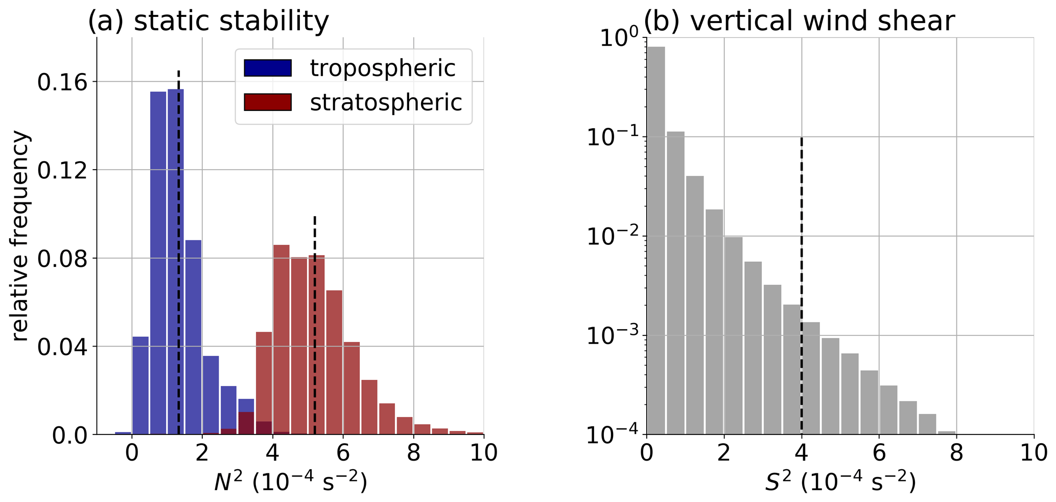
Figure 1Relative occurrence frequency histogram of static stability N2 and vertical wind shear S2 from 1.5 km above the surface up to 25 km altitude on 11 September 2017 at 00:00 UTC over the Northern Hemisphere. Counts are weighted with the grid box volumes. (a) Static stability (N2, in ). Blue indicates values in the troposphere (z<z(LRT)), and red values in the stratosphere (z<z(LRT)). Dashed black lines indicate average tropospheric/stratospheric N2. (b) Relative occurrence frequency distribution of vertical wind shear (S2, in ). Logarithmic occurrence frequency scale. Dash black line indicates threshold value .
We will start our analysis by initially focusing on a specific time step in September 2017. This study was performed in the context of the airborne research campaign WISE that took place during SON 2017 over the North Atlantic, which motivated the choice of the date. Our intention is to introduce our metrics first and then look at longer time periods afterwards. We start with the synoptic situation to provide the large-scale overview. Figure 2 shows a snapshot of the northern hemispheric potential temperature at LRT altitude on 11 September 2017, along with maxima of the horizontal wind at 200 hPa. The primary feature standing out is the tropopause break and the associated jet streaks of the horizontal wind. Over the Asian continent and reaching to the western Pacific, the tropopause break features a sharp meridional Θ(LRT) gradient with a single coherent STJ. Further west, the tropopause break is less sharp and features a characteristic sequence of Rossby wave patterns accompanied by individual jet streaks at varying latitudes.
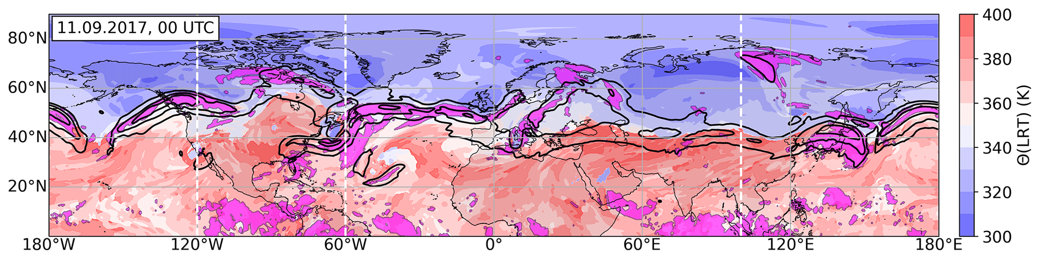
Figure 2Potential temperature at the LRT (Θ(LRT), in K) over the Northern Hemisphere on 11 September 2017 at 00:00 UTC. Black lines show contours of the horizontal wind at 200 hPa, beginning at 30 m s−1 in steps of 15 m s−1. Magenta-shaded areas indicate regions between 1 km below and 2 km above the local LRT. Dashed white lines indicate the location of the vertical cross sections in Fig. 3.
The synoptic-scale wind systems are further illustrated in the vertical cross sections in Fig. 3. At 120∘ W (Fig. 3a), a pronounced polar jet maximum is visible at 50–60∘ N, which is also evident in the 200 hPa horizontal wind in Fig. 2. Further southward, the tropopause break at 30∘ N features comparatively weak westerly winds, followed by high-altitude easterlies in the tropics. The western North Atlantic (Fig. 3b) exhibits two distinct zonal west-wind maxima, which can be interpreted as the jet exit region of the STJ and the entry region of a jet streak of the PFJ. The cross section at 100∘ E (Fig. 3c) again shows a sequence of zonal winds, with high-altitude easterlies in the tropics, followed by the STJ, and further northward the rotational components of a cyclonic system over Siberia.
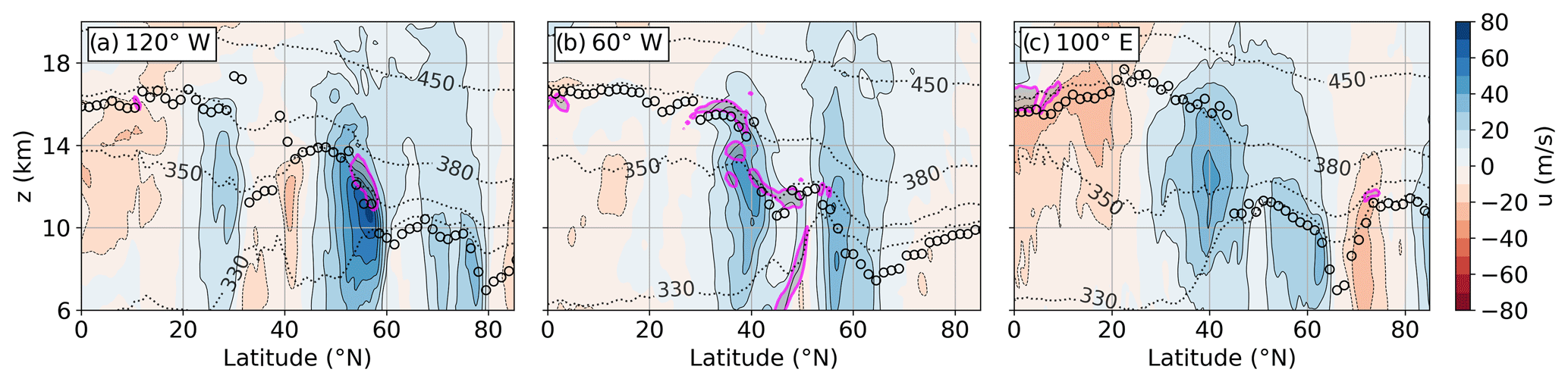
Figure 3Vertical cross sections on 11 September 2017 at 00:00 UTC at (a) 120∘ W, (b) 60∘ W, and (c) 100∘ E. Color contour shows zonal wind speed (u, in m s−1), black dots LRT altitude, and dotted black lines isentropes (Θ, in K). Magenta lines show isolines.
We proceed with the analysis of the vertical and geographical distribution of strong vertical wind shear exceeding the threshold value . Figure 4 shows the zonally averaged relative occurrence frequency of strong vertical wind shear on a logarithmic color scale for the Northern Hemisphere on 11 September 2017. Figure 4a reveals three meridional regions of exceptional occurrence frequencies located in the UTLS region: one in the tropics, one at 30–40∘ N, and a third one at midlatitudes. Rearranging the grid volumes in a tropopause-relative vertical coordinate system depending on their vertical distance from the LRT (Fig. 4b and c) concentrates the maxima of strong wind shear occurrence in all three regions in a vertical layer of about 1–2 km in extent directly above the LRT. Secondary occurrence frequency maxima can be identified closely below the tropopause in all three meridional regions.
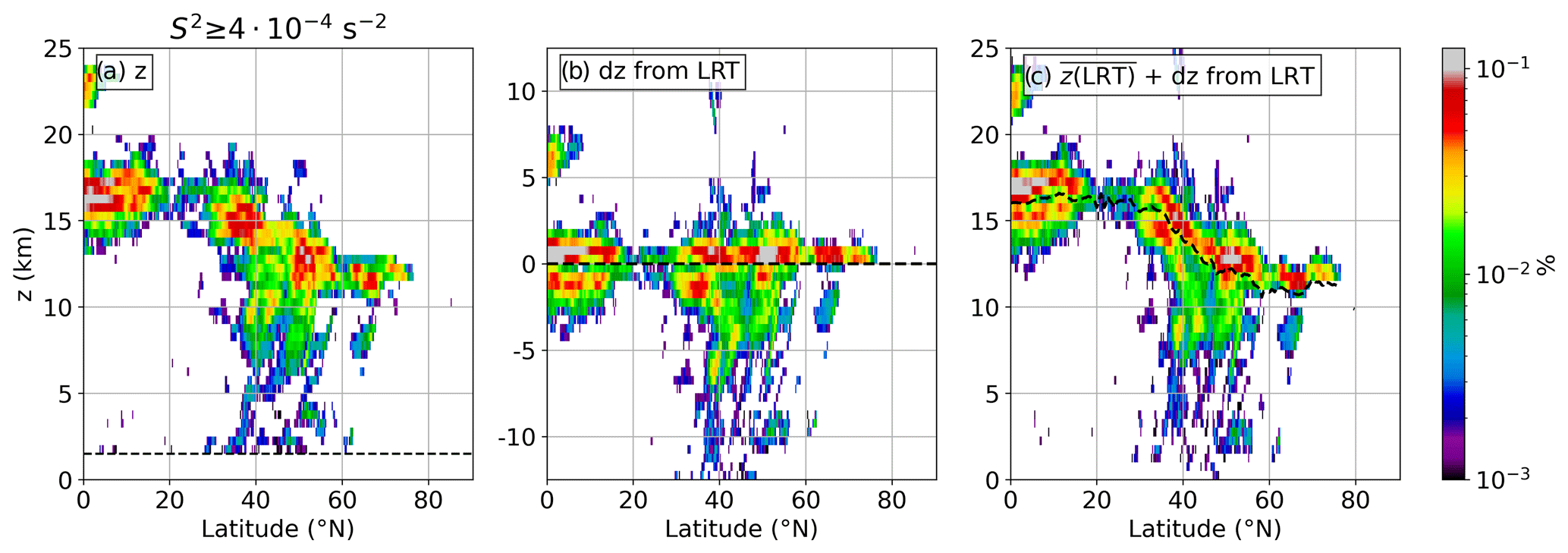
Figure 4Relative occurrence frequency of , zonally averaged over the Northern Hemisphere on 11 September 2017 at 00:00 UTC. Logarithmic frequency contour, vertically binned in dz=500 m. (a) Geometric altitude as the vertical coordinate. Dashed black line indicates the effect of the cut-off of 1.5 km above orography. (b) Relative distance from the LRT as the vertical coordinate. Dashed black line shows LRT altitude. (c) As in panel (b) but with mean LRT altitude for profiles with restored (dashed bold black line).
The pronounced occurrence of in a distinct layer close to the LRT is motivation to proceed with the analysis, focusing on the question, is there a global relation between vertical wind shear and the tropopause? To answer this question, we choose a binary criterion where we define the tropopause region as being exposed to strong vertical wind shear if S2 exceeds at least at one level between 1 km below and 2 km above the LRT. These regions are indicated in Fig. 2. The wind systems described in the first paragraph of this section can now be associated with the three meridional regions of frequent occurrence of strong vertical wind shear near the tropopause in Fig. 4. At midlatitudes, the tropopause region is exposed to strong vertical wind shear within the Rossby wave jet streaks, as well as in the cyclonically curled-up ridges associated with breaking baroclinic waves (over Canada, Scandinavia, and Siberia) (Kaluza et al., 2019). Further southward, the STJ also features strong vertical wind shear at the tropopause, particularly in the jet exit region over the western North Pacific. The tropical easterlies over the Indian Ocean and the east Pacific feature large-scale coherent regions of strong vertical wind shear close to the tropopause. Several smaller-scale wind shear regions can be attributed to individual atmospheric wind systems, e.g., the late-stage ex-hurricane Irma, which is located over Florida, or the stratospheric cut-off over the Mediterranean Sea.
4.1 Vertical distribution and seasonality of strong vertical wind shear in the Northern Hemisphere
We repeat the analysis steps from Sect. 3 for the whole dataset of 10 years of daily ERA5 fields. We first present the overall vertical distribution of strong vertical wind shear , followed by the geographic occurrence frequency and seasonality in the tropopause region.
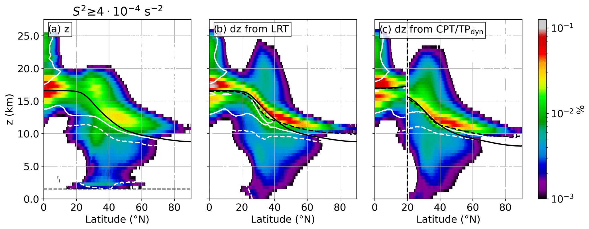
Figure 5Northern hemispheric occurrence frequency distribution of grid volumes that exhibit strong vertical wind shear , from 1 January 2008 to 31 December 2017. Logarithmic frequency contour, vertically binned with dz=500 m. (a) Geometric altitude as the vertical coordinate. Solid bold black line indicates mean LRT altitude for all 10 years and the whole Northern Hemisphere. Dashed thin black line indicates the effect of the cut-off of 1.5 km above orography. Solid (dotted) white line indicates where decreasing (increasing) horizontal winds with altitude constitute 75 % of the strong vertical wind shear . (b) As in panel (a) but with a LRT-relative vertical coordinate and with mean LRT altitude for profiles with restored (dashed bold black line). Solid bold black line as in panel (a). (c) As in panel (b) but from 0–20∘ N with the cold-point tropopause (CPT) as a reference altitude, and north of 20∘ N with the dynamic tropopause (Q=2 pvu) as a reference altitude.
Figure 5a shows the 10-year temporal and zonal average occurrence frequency for strong vertical wind shear , with the geometric altitude as the vertical coordinate. The mean LRT altitude for the same time period and region is indicated by the solid black line. Distinct occurrence frequency maxima are apparent in the midlatitudes between 40–60∘ N mainly above the LRT, at the tropopause break at about 30∘ N above and below the LRT, and in the tropics in close vicinity above and below the LRT. The rearrangement of the grid boxes in the LRT-relative vertical coordinate system (Fig. 5b) concentrates the occurrence frequency maxima in a distinct layer above the LRT. This layer spans from the tropics to latitudes north of 60∘ N, and it exhibits occurrence frequencies on the order of 1 %–10 % over a vertical range of about 1–2 km.
In the following we will refer to the feature of maximum occurrence frequencies near the LRT in the zonal and/or temporal mean as a tropopause shear layer (TSL); however, a comparison with the TIL should be made cautiously. Both features appear similarly in tropopause-relative zonal means (compare with Zhang et al., 2019); however, the wind shear layer emerges less frequently as well as less area-wide. Furthermore, a different metric is applied here, which analyzes the tropopause-relative occurrence frequency of a threshold value , instead of directly averaging S2. We refrain from referring to individual regions of strong wind shear at individual time steps as a tropopause wind shear layer, because this would raise the question of a lower limit for the horizontal and temporal scales that mark such a layer, considering the pronounced mesoscale variability of these regions. We realize that this choice is controversial, because in a mesoscale horizontal extent on the order of 100 km the geometric aspect ratio between horizontal and vertical extent still clearly describes a layer-like character.
At midlatitudes, the TSL is composed of mostly decreasing wind speeds with height. Northward of about 45∘ N, the profiles which exhibit are on average associated with about 1 km more elevated LRT altitudes compared to the overall zonal average (dashed and solid black lines in Fig. 5b). This indicates the importance of large-scale wave dynamics, particularly the polar jet streaks within ridges of baroclinic waves, which are known to exhibit exceptional wind shear in the tropopause region (Kaluza et al., 2019; Kunkel et al., 2019). The above-average LRT altitudes for profiles with are a unique feature for the higher midlatitudes, as they do not occur in the tropics or the subtropics, which will be further addressed in Sect. 4.2.
At the tropopause break, the TSL is more evenly composed of both decreasing and increasing wind speed with height. This is due to the contribution of enhanced vertical wind shear at the upper edge of the tropopause break and above the jet core, as well as at the lower edge and below the jet core. Furthermore, an enhanced vertical spread of is apparent at the tropopause break in the LRT-relative vertical coordinates (Fig. 5b) compared to the geometric altitude (Fig. 5a). Figure 6 illustrates how this can be explained by the averaging method. Below the jet core of the STJ strong vertical wind shear occurs frequently within tropopause folds (Škerlak et al., 2015), i.e., tongues of stratospheric air that reach south- and downward. Despite the stratospheric characteristics of these air masses, the LRT criterion which requires a mean lapse rate below 2.0 K km−1 over a vertical distance of 2 km is no longer met at some point within the tropopause folds, which is indicated by the dashed black line in Fig. 6. In these cases the LRT is located at the upper edge of the tropopause break and several kilometers above the region of strong wind shear. Eventually, the 10-year temporally and zonally averaged LRT altitude exhibits a smoother transition between the lower and the upper edge of the tropopause break (right panel in Fig. 6), which is caused by short-period as well as seasonal meandering of the tropopause break. The LRT-relative averaging method ultimately shifts the region of strong wind shear downward from the mean LRT altitude, over the distance which was originally determined relative to the instantaneous LRT. An equivalent effect also occurs at the upper edge of the tropopause break as indicated in Fig. 6.

Figure 6Schematical vertical cross section of the tropopause-based averaging method. Left part shows exemplary situation at the tropopause break, and right part the key measures after tropopause-based averaging. Black lines indicate the LRT, and grey lines the dynamic tropopause. Blue lines show isotachs, and the yellow and blue regions indicate regions of enhanced vertical wind shear above and below the jet core.
The tropical region in Fig. 5b features the most pronounced occurrence frequency maximum, exhibiting a larger vertical spread compared to higher latitudes, as well as a distinct secondary maximum below the LRT. The composition of positive and negative vertical wind shear in the tropics exhibits a layered structure, particularly above the LRT, where it is influenced by the quasi-biennial oscillation phase and the elevation of the level of vanishing horizontal wind.
The significance of the processes which result in the occurrence of the TSL remains to be quantified. The clustering of grid volumes which exhibit directly above the LRT in Fig. 5b agrees with the dynamic stability criterion, as well as the thermal wind associated with the baroclinicity at upper-tropospheric fronts. However, the overall link between the tropopause definition, which is governed by the temperature profile, and the occurrence of strong vertical wind shear remains uncertain. Therefore, we repeat the analysis for the tropical CPT – i.e., the absolute temperature minimum in the tropical UTLS – and for the dynamic tropopause, i.e., the Q=2 pvu isosurface in the extratropics. The tropics feature a distinct separation of up to 1 km between the LRT and the CPT (Seidel et al., 2001), which motivates the comparison at low latitudes. The PV on the other hand does not constitute a useful tropopause definition in the tropics (Holton, 1995), which is why the dynamic tropopause is only used in the extratropics in this study. From Fig. 5c it is evident that ERA5 resolves the separation of the LRT and the CPT in the tropics. The clustering of above the CPT is less pronounced compared to the LRT, along with a more pronounced secondary maximum below the CPT, which indicates that the occurrence of strong vertical wind shear is more closely linked to the LRT in the tropics. In the extratropics, the analysis in a vertical coordinate system relative to the dynamic tropopause (Fig. 5c and north of 20∘ N) compares well with the analysis in the LRT-relative vertical coordinates. At high latitudes, the profiles which exhibit strong vertical wind shear are associated with above-average dynamic tropopause altitudes. However, the clustering of grid volumes with above the dynamic tropopause exhibits a larger vertical spread, particularly above the tropopause break. The dynamic tropopause is identified systematically below the LRT in this region. Therefore, a larger amount of grid volumes which exhibit strong wind shear are shifted upwards during the averaging process. In conclusion, the averaging of the grid volumes which exhibit based on the distance from the different reference altitudes reveals that the elevation of strong vertical wind shear is (not generally but in the overall mean) more closely linked to the LRT than to the CPT or the dynamic tropopause.
We proceed with the analysis of the geographical spread of wind shear regions which are located between 1 km below and 2 km above the local LRT. For that, we calculate occurrence frequencies for how often the binary criterion for strong vertical wind shear close to the LRT which was defined in Sect. 3 is met. Figure 7 shows the seasonality of these quasi-horizontal occurrence frequencies over the Northern Hemisphere. Throughout all seasons, a clear separation of occurrence frequency maxima is apparent, where each region can be attributed to a planetary circulation feature. The eastern North Pacific and the North Atlantic each exhibit a distinct maximum spanning over the storm track regions (Shaw et al., 2016). These maxima are most pronounced during winter and spring, exhibiting maximum occurrence frequencies of 25 %–30 %.
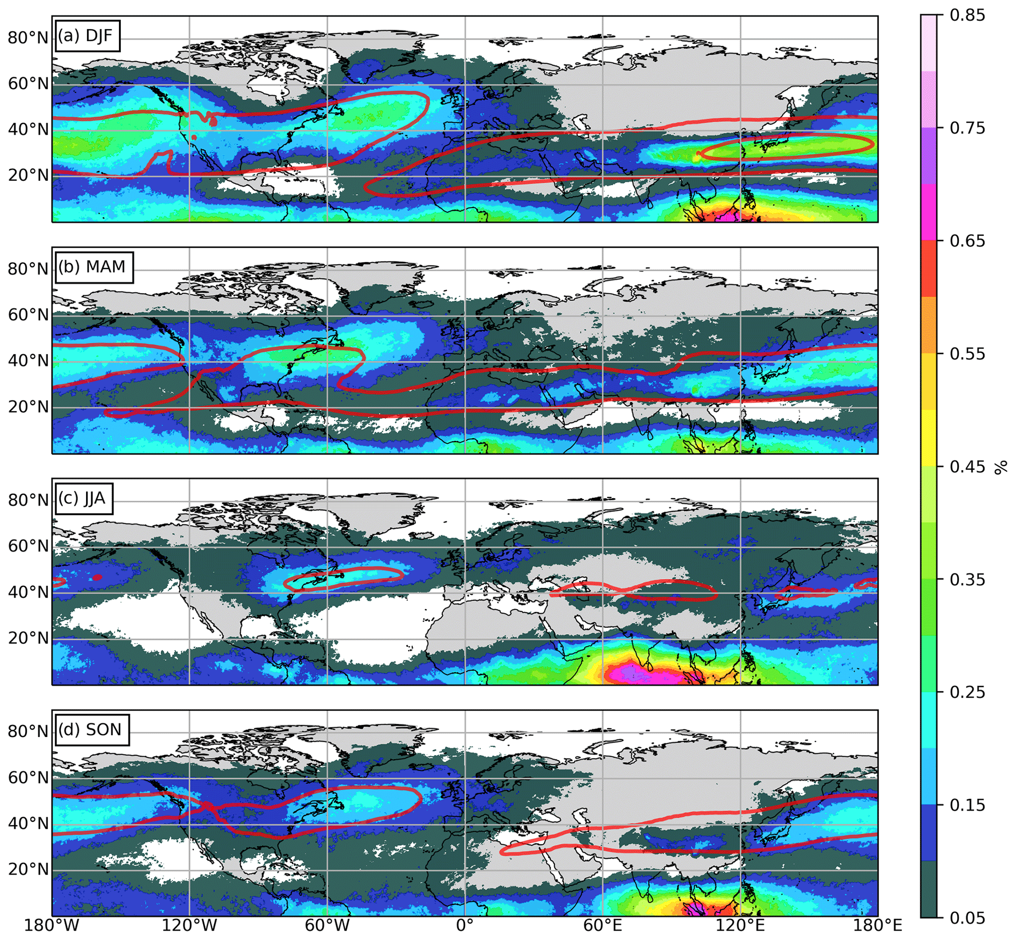
Figure 7Occurrence frequency distribution of between 1 km below and 2 km above the local LRT in the Northern Hemisphere. Averaged over 10 years from 2008 to 2017 for (a) DJF, (b) MAM, (c) JJA, and (d) SON. Solid red lines indicate isolines of the horizontal wind at 200 hPa, starting at 30 m s−1 in steps of 30 m s−1.
Another region with maximum occurrence frequencies of up to 45 % is apparent over Asia and the western North Pacific during winter, which is associated with the STJ. The strength of the maximum throughout the year shows a general agreement with the seasonality of the jet stream. The tropics feature several maxima spanning around the Equator, with one particular wind shear region located over the Indian Ocean which exhibits maximum occurrence frequencies up to 75 % during JJA. This maximum shifts eastward during autumn and winter, when it is located over the maritime continent. The summer maximum can be attributed to the emergence of the TEJ during these months, associated with the Asian summer monsoon circulation. The winter maximum is linked to the Pacific Walker circulation and the El Niño–Southern Oscillation (ENSO) ocean–atmosphere coupling. This will be further addressed in Sect. 4.3.
The following subsections each focus on one of the regions where strong vertical wind shear occurs frequently at tropopause altitudes, beginning at high latitudes and moving towards the Equator. The goal is to discuss the relation to planetary circulation features and to investigate formation mechanisms of the TSL in the dataset.
4.2 The TSL related to Rossby waves in the midlatitudes
At midlatitudes, the occurrence of enhanced tropopause-based vertical wind shear is linked to the jet streaks of the PFJ and therefore to the associated baroclinic wave patterns. Figure 5b and c indicated above-average lapse rate and dynamic tropopause altitudes for profiles exposed to , which hints at the role of the ridges of baroclinic waves. This behavior agrees with the conclusions from the process study of Kunkel et al. (2019) as well as the composite study of baroclinic waves of Kaluza et al. (2019). We expect the ERA5 reanalysis to resolve vertical wind shear features in the UTLS similarly well compared to the operational IFS analysis data used in Kaluza et al. (2019). However, a direct comparison should be made carefully. The ERA5 reanalysis is based on an IFS version with a TL639 spectral truncation (about 31 km horizontal grid spacing; see Hersbach et al., 2020) and 137 vertical levels, compared to the TL1279 spectral truncation (about 16 km horizontal grid spacing) and 91 or 137 vertical levels in the operational analysis data used in Kaluza et al. (2019).
The following subsection presents a more detailed analysis of the dependency of strong vertical wind shear on the tropopause altitude.
We begin by selecting two zonal regions encompassing the occurrence frequency maxima in the midlatitudes: one over the North Atlantic from 80 to 0∘ W and a second one over the eastern North Pacific from 180 to 120∘ W. The latter selection is made in such a way as to exclude the STJ maximum to the west. We proceed with the Q=2 pvu isosurface fields provided by the ECMWF and make use of the conservation property of the potential temperature Θ on such an isosurface under adiabatic and frictionless conditions (Hoskins, 1991). We can therefore identify Rossby waves through anomalies of Θ(Q=2 pvu), with positive anomalies indicating a ridge of a baroclinic wave – i.e., subtropical air masses with high tropopause altitudes reaching poleward – and negative anomalies indicating a trough, i.e., polar/subpolar air masses with low tropopause altitudes reaching equatorwards.
We proceed by defining a background state from which we can identify Θ(Q=2 pvu) anomalies. Figure 8a and b show the 10-year temporal and zonal average of the potential temperature for both latitudinal regions and subdivided into DJF, MAM, JJA, and SON. On average, the dynamic tropopause exhibits potential temperatures of about 360 K at 20∘ N and decreases to values between 300–320 K in the polar region. The meridional gradient is most pronounced during DJF and MAM in both regions. We preserve the meridional dependency and define the zonal and temporal average in the meridional region from 35–60∘ N as the background state for the following analysis. According to Fig. 7, this region encompasses the occurrence frequency maxima over the North Atlantic and the eastern North Pacific. Furthermore, Fig. 8a and b show that the interseasonal standard deviation of is generally small in this region, which indicates that the 10-year seasonal average describes representative average potential temperatures at the dynamic tropopause for the individual years. Figure 8c and d show for the zonal mean that the LRT exhibits averaged potential temperatures close to the ones of the dynamic tropopause, particularly in the region of interest from 35–60∘ N. We present this comparison because we make use of both tropopause definitions. On the one hand, we analyze the occurrence of relative to the LRT, because the analysis in Sect. 4.1. showed that strong wind shear is more closely linked to the LRT than to the dynamic tropopause. On the other hand, we identify UTLS wave features on the basis of the dynamic tropopause, because of the conservation property of the PV.
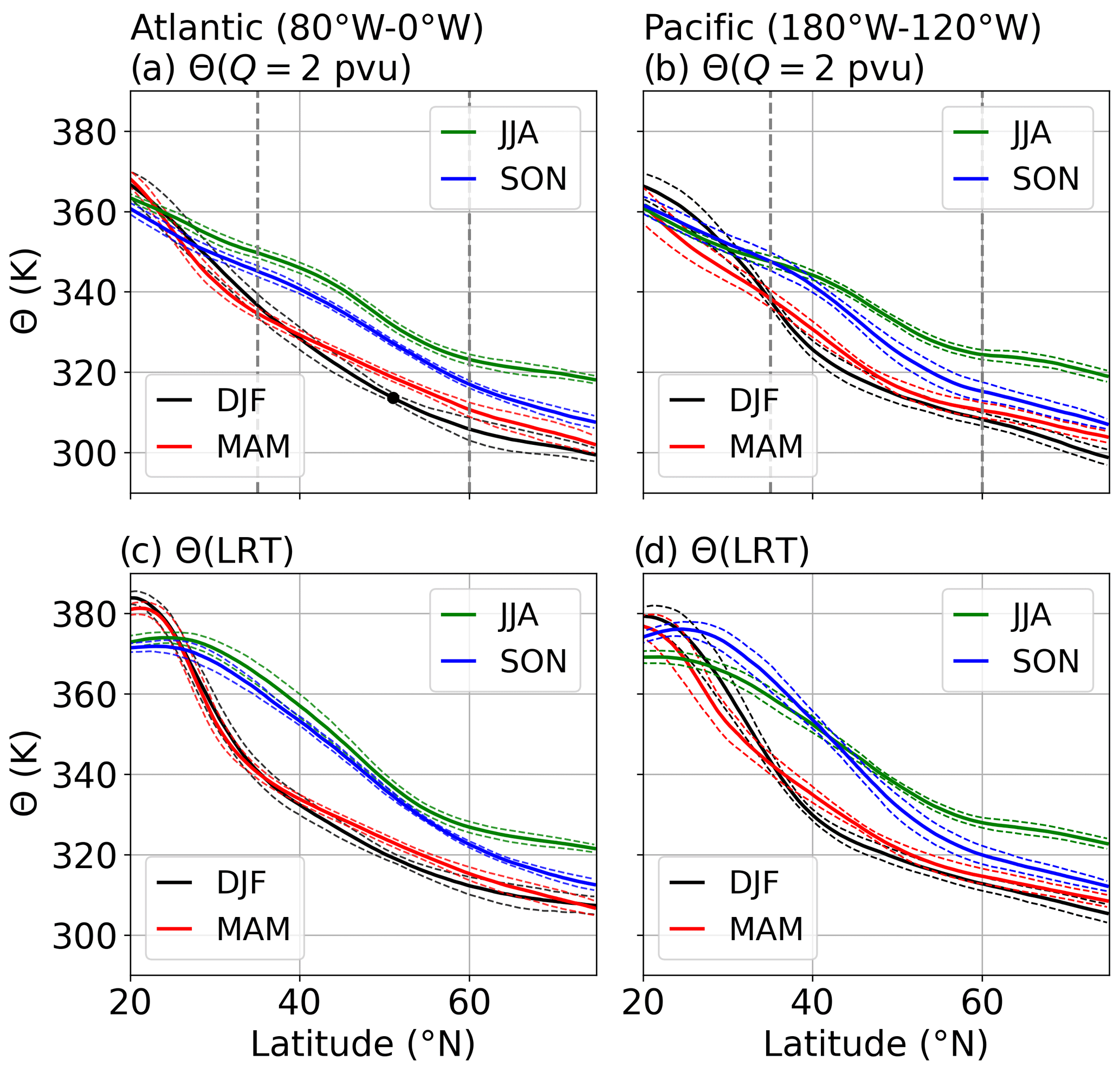
Figure 8(a, b) Seasonal 10-year temporally and zonally averaged dynamic tropopause potential temperature (, in K). (c, d) Seasonal 10-year temporally and zonally averaged LRT potential temperature ( (LRT), in K). Solid lines show mean values, and dashed lines interseasonal standard deviation. Left column North Atlantic region (80–0∘ W). Right column eastern North Pacific region (180–120∘ W). The black dot in panel (a) indicates at 51∘ N, where Fig. 9 is located. Dashed grey vertical lines in panels (a) and (b) indicate the borders of the region that is further analyzed.
We proceed by calculating the distribution of instantaneous deviations from during the 10 years for each region and season. Figure 9 exemplarily shows the result for the North Atlantic region during DJF and at 51∘ N. The Θ(Q=2 pvu) values are unimodally distributed around the 10-year average background value of K. Vertical wind shear exceeding in the vicinity of the LRT, however, occurs almost exclusively at above-average Θ(Q=2 pvu) values. The occurrence frequencies for increase up to 55 % with increasing Θ(Q=2 pvu) up to the point where the occurrence frequencies for the potential temperatures become statistically insignificant.

Figure 9Occurrence frequency of within 1 km vertical distance from the LRT, depending on Θ(Q=2 pvu). Blue histogram shows occurrence frequency distribution of Θ(Q=2 pvu) at 51∘ N during DJF in 2008–2017 and averaged over 80–0∘ W. Θ(Q=2 pvu) in 1 K bins. Dashed black line shows mean value K (black dot in Fig. 8a). Solid black line shows occurrence frequency for between 1km below and 2 km above the local LRT and within the Θ(Q=2 pvu) bins.
Figure 10 presents the extension of the previous analysis for both regions, all seasons, and over the whole selected meridional range. Figure 10a puts the result from Fig. 9 into a larger context and reveals that in the vicinity of the LRT is generally associated with positive ΔΘ(Q=2 pvu) anomalies, i.e., dynamic tropopause potential temperatures above the climatological mean, i.e., primarily ridge regions. The occurrence frequencies increase with increasing potential temperatures and at higher latitudes, with peak values exceeding 50 % at about 50∘ N and K.
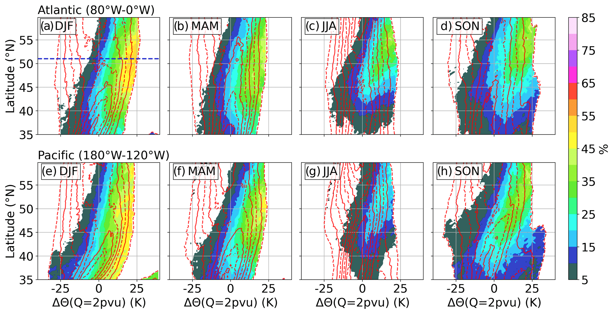
Figure 10Occurrence frequency of ΔΘ(Q=2 pvu) deviations from as in Fig. 8c, with meridional dependency. Dashed (solid) red lines indicate occurrence frequencies isolines, beginning at 0.5 % (1.0 %) and in steps of 1.0 %. Color contour shows occurrence frequency for between 1 km below and 2 km above the local LRT and within the Θ(Q=2 pvu) bins. (a–d) DJF, MAM, JJA, and SON over the North Atlantic region. (e–h) Same for the Northeast Pacific region. Dashed blue line in panel (a) indicates location of Fig. 9.
The general dependency for the occurrence frequency of in the latitude–ΔΘ(Q=2 pvu) coordinates holds true for both regions and all four seasons, with overall reduced values towards the summer months, accompanied by a northward shift. In the eastern North Pacific region and particularly during DJF, the influence of the STJ is visible, causing the bimodal distribution of ΔΘ(Q=2 pvu) at low latitudes. This is due to occasional northeastward excursions of the STJ and the subtropical tropopause break into the region of interest, which adds exceptionally high dynamic tropopause potential temperatures to the statistic and shifts the overall average towards larger values.
The following consideration is made to put the results of the previous paragraphs in context. From a static point of view and according to Fig. 7a, maximum occurrence frequencies for in the vicinity of the LRT over the North Atlantic and during DJF are located at about 50∘ N and reach up to values of 30 %–35 %. From a dynamic point of view, the occurrence can be further narrowed down, with occurrence frequencies exceeding 45 % within any elevated tropopause between 80–0∘ W and 45–55∘ N that exhibits ΔΘ(Q=2 pvu)≳20 K. The northward excursion of air masses exhibiting above-average tropopause altitudes within ridges of baroclinic waves and the associated jet streaks can be expected to be mainly responsible for this correlation.
Overall, the analysis presents one way to quantify the link between the occurrence of strong vertical wind shear near the tropopause and the potential temperature of the dynamic tropopause, which can be interpreted as a measure for the excursion of air masses within baroclinic waves in the midlatitudes.
4.3 The TSL around the subtropical jet stream and in the tropics
4.3.1 The east Asian jet stream
The tropopause region over east Asia and the western North Pacific features a maximum in occurrence frequencies for , which is associated with the STJ (Fig. 7). The STJ in this region is most pronounced during DJF, when it is also referred to as the east Asian jet stream (EAJS; Yang et al., 2002). Figure 11 shows the zonal and 10-year seasonal average of the potential temperature Θ at the LRT for DJF and JJA, as well as the associated occurrence frequency of between 1 km below and 2 km above the local LRT. The meridional course of Θ(LRT) agrees well with the climatology derived from radiosonde measurements by Seidel et al. (2001). During winter, the zonally averaged occurrence frequency maximum for is located right at the meridional location of the tropopause break and exhibits values of up to 25 % at around 30∘ N. The strength of the occurrence frequency maximum exhibits a pronounced interseasonal standard deviation of 5 % (absolute values), which can be partly linked to variability features of the EAJS. The meridional location of the occurrence frequency maximum is rather sharply defined, in agreement with the stable meridional location of the EAJS core on interannual timescales (Yang et al., 2002). The zonal location of the jet core, however, exhibits a comparatively large interannual variability (Wu and Sun, 2017), which can be linked to the interseasonal variability of the occurrence frequency of in Fig. 11a. In the time period analyzed by Wu and Sun (2017) that intersects with our analysis, they find the EAJS core to be located comparatively far westward during the winter seasons of 2008, 2011, and 2012, accompanied by large maximum EAJS core wind speeds. According to Fig. 12a, these years feature exceptionally large occurrence frequency maxima centered within the zonal region from 60–180∘ E. In contrast, the 2009 and 2010 EAJS core is located further eastward and exhibits lower maximum wind speeds, along with reduced occurrence frequencies for (Fig. 12b). Note that the zonal location of the jet core is not well reflected in the multiannual mean of the horizontal wind at 200 hPa. The link between the occurrence of strong vertical wind shear near the tropopause and the location and strength of the jet core should not be generalized and needs further investigation, since, for example, Wu and Sun (2017) do not see a strong correlation between the zonal EAJS core location and maximum wind speeds. Furthermore, it should be kept in mind that the occurrence of in the vicinity of the LRT is not necessarily linked to exceptional jet core wind speeds.

Figure 11Vertical cross sections of 10-year average tropopause properties between 60 and 180∘ E longitude: (a) winter (DJF) and (b) summer (JJA). Upper panels: solid black line shows (LRT) for the zonal region. Solid blue line shows zonally averaged occurrence frequency for between 1 km below and 2 km above the local LRT, and dashed solid line depicts (LRT) for such vertical profiles. Bottom panels show interannual standard deviation for every measure. The standard deviation of the occurrence frequency displays absolute percentage values.

Figure 12As in Fig. 7a but for a smaller geographical section, averaged over selected DJF seasons of (a) west-located EAJS core years (2008, 2011, and 2012) and (b) normally located EAJS core years (2009 and 2010). For further details see text and Wu and Sun (2017).
Towards summer, the jet stream slows down and shifts to the north of the upper-tropospheric Tibetan high-pressure system associated with the east Asian summer monsoon (EASM) circulation. The zonally averaged occurrence frequency maximum for in the vicinity of the LRT during JJA decreases to 11 % and is centered at the upper edge of the tropopause break (Fig. 11b).
4.3.2 The tropical easterly jet
In the tropics, the summer maximum over the Indian Ocean (Fig. 7c) is associated with the TEJ. These easterlies generally arise from June to September as part of the EASM circulation at upper-tropospheric pressure levels around 150 hPa (Krishnamurti and Bhalme, 1976). Fig. 11b shows the zonally averaged occurrence frequency for close to the LRT encompassing the TEJ summer maximum. It exhibits a significant interannual variability, a feature also seen in the vertical shear of the zonal wind found by Roja Raman et al. (2009) at different heights above the TEJ core using MST radar and GPS radiosonde measurements. Furthermore, the occurrence frequencies for strong vertical wind shear which were derived from radiosonde measurements by Sunilkumar et al. (2015) agree qualitatively with the ones at the respective geographic location of each radiosonde station in Fig. 7c. The authors analyzed, among other things, occurrence frequencies for vertical wind shear threshold values, albeit not in a tropopause-relative coordinate system and with gradients calculated within sampling windows of 20 m (implicating a larger spectrum of resolved wind shears compared to ERA5), which should be considered when comparing the results. The radiosonde data revealed occurrence frequencies during the monsoon season (June–September) for of almost 80 % at Trivandrum (8.3∘ N, 76.6∘ E) and 67 % at Gadanki (13.5∘ N, 79.2∘ E) and for occurrence frequencies of 37 % at Trivandrum and 15 % at Gadanki. These peak values occur as sharp maxima above the convective tropopause and close to the CPT, where the LRT is generally located in between (Sunilkumar et al., 2013).
4.3.3 The winter Pacific Walker circulation cell
During the winter months, the tropical tropopause region features another pronounced occurrence frequency maximum for eastward of the summer TEJ maximum and centered over the maritime continent (Fig. 7a). It is associated with localized upper-tropospheric easterlies and exhibits a smaller zonal extent as well as about 5 %–10 % lower maximum occurrence frequencies in the 10-year average compared to the summer TEJ maximum.
The pronounced interannual variability in the zonally averaged occurrence frequencies for (Fig. 11a), as well as the geographic location of the maximum and the season of its occurrence, indicates a link to the ENSO ocean–atmosphere coupling and the effect on the Pacific Walker circulation cell. To test this hypothesis, we select a region encompassing the shear occurrence frequency maximum, from 100 to 130∘ E and from the Equator to 10∘ N, and calculate the average occurrence frequency of close to the LRT in this region during DJF and for the individual years. The comparison of these time- and area-averaged frequencies with the Oceanic Niño Index (ONI) sea surface temperature anomaly values for DJF shows an anticorrelation (Fig. 13a), with a Pearson correlation coefficient of . The analysis reveals moderate to large occurrence frequencies during neutral and La Niña conditions and a peak during DJF 2010/11, a year of strong La Niña manifestation. The positive sea surface temperature anomaly in the west Pacific is accompanied by increased convection over the maritime continent, which results in enhanced upper-tropospheric outflow and a strengthening of the adjacent Walker circulation cell (Fig. 13c). Still, the frequent occurrence of strong vertical wind shear near to the LRT is striking, considering the still comparatively weak easterlies. The occurrence of strong vertical wind shear near the tropopause could be influenced by enhanced gravity wave activity associated with deep convection (Podglajen et al., 2017), as convection is the major source for gravity wave generation in the tropics through several forcing mechanisms (Müller et al., 2018, and references therein). During the pronounced El Niño winter seasons 2009/10 and 2015/16 the shear occurrence frequency decreases to values in the range of 30 %–40 %, which is significantly below the 10-year average value of 54.2 %. This is associated with the eastward shift of the less sharply defined rising branch of the Pacific Walker circulation cell (Sullivan et al., 2019), along with the less pronounced upper-tropospheric easterlies (Fig. 13b).
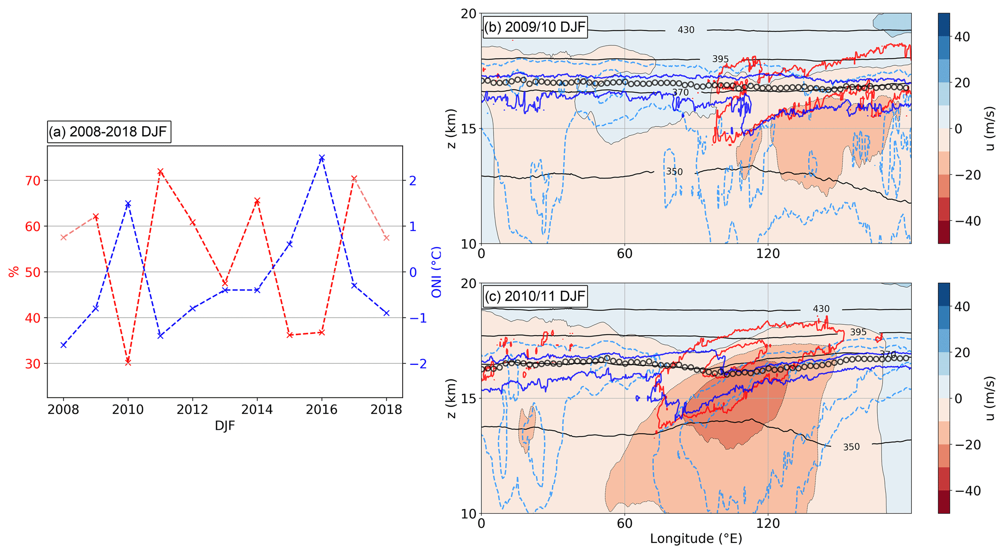
Figure 13(a) Comparison of the Oceanic Niño Index sea surface temperature anomaly for DJF (ONI, blue graph) with the strong shear occurrence frequency during DJF averaged over the region from 100 to 130∘ E and from the Equator to 10∘ N (red graph). The values for January–February 2008 and December 2017 are included (light red). ONI values from https://www.noaa.gov/ (last access: 16 July 2021). (b, c) Temporal mean of a zonal cross section at the Equator, averaged in geometric height coordinates, for the two consecutive DJF seasons 2009/10 and 2010/11. Color contour shows mean zonal wind component (u, in m s−1). Solid red lines show the 10 % and the 50 % isolines of occurrence frequencies for . Solid blue lines show the 10 % and the 50 % isolines of occurrence frequencies for . Black circle markers indicate LRT altitude, and solid black lines show isolines of potential temperature (Θ, in K). Dashed light blue lines indicate the isolines of 70 % and 85 % relative humidity over ice.
We now briefly revert to Fig. 5b and the secondary occurrence frequency maximum for below the tropical LRT, which is strikingly separated from the one above. This secondary maximum emerges due to a comparable situation to the one described for the secondary maxima at the subtropical tropopause break (Fig. 6), only on smaller scales and zonally aligned. The following explanation is applicable to both the TEJ and the winter Walker cell easterlies. We will focus on the latter to give an exemplary explanation. The easterlies responsible for the DJF TSL occurrence frequency maximum are associated with a frequently occurring lapse rate tropopause jump of 0.5–1.0 km vertical distance, located at the western edge of the easterlies (Fig. 13c). This is indicated by the occurrence frequency isolines for . These regions of enhanced static stability reach west- and downward, where at some point they no longer fulfill the definition of the LRT criterion, causing the tropopause jump. The tropopause-based averaging method then results in a secondary occurrence frequency maximum for below the LRT, due to enhanced wind shear within the regions of enhanced N2 that reach below the local LRT.
The TSL and particularly its relation to the TIL owe their potential importance to the fact that both the TSL and the TIL majorly influence the dynamical stability and may be related to the formation of the extratropical transition layer (ExTL), which is derived from observations of chemical tracers (e.g., Hoor et al., 2002; Pan et al., 2004). Related to that, the potential implications of the frequently occurring TSL within the tropical tropopause layer (TTL; Fueglistaler et al., 2009) need further investigation.
It is important to analyze the relation of the TSL and the TIL in more detail, because both co-occur as climatological features in zonal and/or temporal tropopause-based averages (e.g., Birner et al., 2002; Birner, 2006; Grise et al., 2010; Zhang et al., 2019). However, we see no general co-location of enhanced N2 and enhanced S2 above the local lapse rate tropopause in instantaneous considerations and on smaller scales. Figure 14a shows the relative occurrence frequency of N2–S2 pairs for all 10 years and in the region between the LRT and 3 km above. The majority of grid volumes exhibit a static stability between the stratospheric background and enhanced values associated with the TIL. At the same time, comparatively “weak” vertical wind shear is most prevalent. Vertical wind shear and static stability do not correlate, and enhanced values of S2 can be found within a large spectrum of N2 under the condition that dynamic stability Ri>Ric is (for the most part) maintained. Particularly the largest values of N2 and S2 do not correlate. Ultimately this has consequences for the dynamic stability of the flow, along with the potential for turbulence and mixing across and above the tropopause. In the case of baroclinic waves in the North Atlantic storm track region, Kaluza et al. (2019) described a co-occurrence of the TIL and tropopause-based enhanced vertical wind shear in cyclone-based composites. This indicates that the processes responsible are active in the same region on a synoptic scale, i.e., ridges. These processes, however, have a different impact on the temperature and momentum profiles. The vertical divergence of the vertical wind in the anticyclonic flow sharpens the temperature profile (Wirth, 2003, 2004), as well as long- and shortwave radiative effects due to trace gas and cloud ice water gradients at the tropopause (Randel et al., 2007; Kunkel et al., 2016), where the latter is particularly important in the context of warm conveyor belts and high-reaching cloud formation in the tropospheric flow within ridges (Madonna et al., 2014).
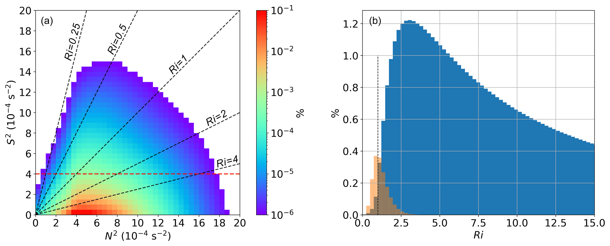
Figure 14(a) Relative occurrence frequency distribution of N2–S2 pairs in the region between the LRT and 3 km above for all daily northern hemispheric ERA5 fields from 2008–2017. Logarithmic occurrence frequency color scale. Dashed red line indicates . Dashed black lines indicate the Richardson numbers 0.25, 0.5, 1.0, 2.0, and 4.0. (b) Histogram of the relative distribution of Richardson numbers associated with the data displayed in panel (a). Orange bars show Ri for grid volumes with , and blue bars for the remaining grid volumes between the LRT and 3 km above. Dotted black line indicates Ri=1.
On sub-synoptic scales, gravity waves can have a large influence on both N2 and S2 above the tropopause (e.g., Kunkel et al., 2014), albeit according to linear wave theory with a phase shift of between the perturbation of the horizontal wind in the direction of the horizontal wave vector and the perturbation of the temperature (Suzuki et al., 2010), and a resulting shift between N2 enhancement and S2 enhancement (compare, e.g., Kunkel et al., 2014). Recently, Podglajen et al. (2020) compared long-duration superpressure balloon measurements with Lagrangian trajectories calculated from a set of numerical reanalysis products and were able to show that the ERA5 reanalysis resolves central features of the gravity wave spectrum. The underlaying IFS model resolves low-frequency large-scale gravity waves down to wavelengths which approach the effective resolution, which is generally estimated to exhibit a factor of about 10 compared to the effective grid spacing. The assimilation of high-resolution observational data further enhances the gravity wave activity in the model. Furthermore, Krisch et al. (2020) identified individual wave packets in the ERA5 data that had been observed with the Gimballed Limb Observer for Radiance Imaging of the Atmosphere (GLORIA) during the GW-LCYCLE airborne measurement campaign. While these studies confirm that modern reanalysis products are capable of resolving central features of the gravity wave spectrum, the overall wind variability due to gravity waves is likely still underestimated in the ERA5. Recently, Schäfler et al. (2020) reported a significant underestimation of the vertical wind shear near the tropopause in the IFS, based on a comparison of Doppler wind lidar measurements with IFS analysis and forecast data. The model errors were most prominent at elevated tropopause altitudes above upper-tropospheric ridges, i.e., regions that contribute significantly to the occurrence of the TSL in the extratropics.
Another issue that needs further investigation is the relation between the TSL and the occurrence of turbulence and potential STE. The grid volumes with in Fig. 14a are mostly located below the diagonal dashed black line which indicates Richardson numbers of Ri=1. The corresponding relative distribution of Richardson numbers is shown in Fig. 14b. The distribution peaks at Ri=3 and spans over a large spectrum of larger Richardson numbers (only a section of the distribution is displayed). Richardson numbers of Ri<1 are rarely associated with vertical wind shear . This indicates that the lowermost stratosphere up to 3 km above the LRT is dynamically stable in the absence of strong vertical wind shear. In contrast, a significant proportion of grid volumes which exceed in Fig. 14a are located above the Ri=1 isoline. These grid volumes constitute the greater part of Richardson numbers Ri<1 within the first 3 km above the LRT, which is indicated in Fig. 14b.
We define the TSL as an occurrence frequency maximum for strong vertical wind shear in tropopause-relative zonal and temporal averages. This occurrence frequency maximum is composed of individual localized shear patches that emerge above the LRT, as the exemplary cross sections in Fig. 3 show, resulting in reduced Richardson numbers on the order of 1 in the elsewhere dynamically stable lower stratosphere. Strong wind shear does not correlate well with the occurrence of turbulence (e.g., Knox, 1997) because it does not necessarily imply dynamic instability, but it is a prerequisite for dynamic instability to occur. Thus, the occurrence frequency distribution presented in Fig. 5a narrows down the region where turbulence due to dynamic shear instability can be expected above the tropopause. The vertical confinement within a few kilometers above the lapse rate tropopause indicates a link to the chemically defined ExTL or mixing layer. Airborne in situ measured carbon monoxide (CO) profiles in the tropopause region exhibit a distinct “kink” in the vertical transition from tropospheric to stratospheric values, which defines the upper edge of a chemical transition layer. Hoor et al. (2004) determined it to be located at about 25 K potential temperature above the Q=2 pvu dynamic tropopause, or 2–3 km above the lapse rate tropopause at high latitudes according to Pan et al. (2004). Hegglin et al. (2009) expanded these results onto a global scale based on CO-O3 and H2O-O3 tracer–tracer correlations derived from ACE-FTS satellite data. Berthet et al. (2007) used a statistical approach on Lagrangian trajectories that were subjected to troposphere-to-stratosphere transport (TST), with their trajectory model being driven by operational ECMWF analysis data. The relative contribution of TST trajectories showed a largely tropopause-following behavior with a limited vertical extent, indicating the amount and vertical reach of the permeability of the transport barrier that is the tropopause. Hoor et al. (2010) continued the Lagrangian approach and linked the chemical transition layer to troposphere–stratosphere transition transport timescales in the range of 0–50 d, which is short compared to the transport timescales in the LMS above the ExTL. The vertical confinement of the TSL may contribute to the separation of the LMS, with a lower layer being frequently affected by shear-driven turbulent STE (e.g., Spreitzer et al., 2019; Kunkel et al., 2019). The TSL properties indicate its role as a contributing mechanism for the formation and maintenance of the ExTL, along with other known processes like radiation-induced PV modifications (Zierl and Wirth, 1997) or convective injection of tropospheric air (Homeyer et al., 2014).
The goal of this study was to investigate the occurrence of strong vertical wind shear in the UTLS region. It was motivated by the wide range of research studies that describe the occurrence of strong vertical wind shear at the tropopause. This includes case studies on turbulent stratosphere–troposphere exchange (e.g., Shapiro, 1976, 1978; Whiteway et al., 2004; Kunkel et al., 2019), climatological studies on the TIL (Birner et al., 2002; Birner, 2006) and its interaction with gravity waves (Zhang et al., 2015, 2019), studies on planetary circulation features (Sunilkumar et al., 2015), and numerical model data studies (Kunkel et al., 2014; Liu, 2017; Kaluza et al., 2019; Spreitzer et al., 2019). However, there was a lack of a comprehensive statistical analysis of this atmospheric feature in a global and climatological sense. We approached this matter using 10 years of data of daily northern hemispheric ECMWF ERA5 reanalysis fields.
Strong vertical wind shear was selected based on the threshold value . A single day analysis introduced the metrics and exemplified that strong vertical wind shear exceeding the threshold occurs nearly exclusively in close vertical vicinity above the lapse rate tropopause. It furthermore showed that the strong vertical wind shear near the tropopause can generally be attributed to planetary circulation features, i.e., polar jet streaks within differently evolved baroclinic waves, the subtropical jet stream, and the upper-tropospheric easterlies of the Walker circulation cells.
The 10-year temporally and zonally averaged meridional cross section revealed a tropopause shear layer (TSL), which is defined by an occurrence frequency maximum on the order of 1 %–10 % for strong vertical wind shear near the tropopause. These occurrence frequencies are about an order of magnitude larger than anywhere else in the region analyzed. The TSL is vertically confined to the first 1–2 km above the lapse rate tropopause and spans from the tropics down to high latitudes around 70∘ N. The geographical mapping of the TSL revealed distinctly separate regions of preferred occurrence, which can each be linked to individual planetary circulation features:
-
The storm track regions over the North Atlantic and the eastern North Pacific feature distinct occurrence frequency maxima for enhanced tropopause-based vertical wind shear. These maxima are most pronounced during DJF and are associated with jet streaks of the eddy-driven jet. The enhanced tropopause-based vertical wind shear emerges at above-average tropopause altitudes associated with ridges of baroclinic waves. We identified the northward excursion of air masses within ridges on the basis of deviations of the potential temperature at the dynamic tropopause from the 10-year temporal and zonal average within each region. The occurrence frequencies for strong vertical wind shear near the tropopause peak at latitudes around 50∘ N and reach values up to 50 % for profiles associated with above-average dynamic tropopause potential temperatures of ΔΘ≈20 K.
-
The east Asian jet stream during winter exhibits occurrence frequencies of up to 45 % for strong vertical wind shear near the tropopause, with a pronounced interannual variability. This appears to be linked to the variability in strength and location of the jet stream (Wu and Sun, 2017), which needs further investigation.
-
The lapse rate tropopause region above the summer tropical easterly jet is up to 70 % of the time exposed to strong vertical wind shear near the tropopause and over a large area of the Indian Ocean. These very striking occurrence frequency maxima and their interannual variability agree well with results from observation-based research studies (Roja Raman et al., 2009; Sunilkumar et al., 2015).
-
The winter Walker circulation easterlies over the maritime continent exhibit an occurrence frequency maximum for strong vertical wind shear near the tropopause which is comparable to the one associated with the tropical easterly jet. The strength and zonal location of these easterlies are closely linked to the El Niño sea surface temperature anomaly and the shift in the Walker circulation. The area-averaged occurrence frequencies for strong vertical wind shear near the tropopause above the maritime continent show a pronounced interseasonal variability, ranging from 30 %–40 % during the El Niño phases in the winter seasons 2009/10 and 2015/2016 up to 70 % during the strong La Niña phase 2010/11.
Overall, this analysis presents a step towards a better understanding of the dynamical structure of the transition region between the troposphere and the stratosphere, i.e., the ExTL in the extratropics and the TTL in the tropics. The occurrence of the TSL can have several implications:
-
The TSL could be an indicator for the efficiency of the processes responsible for its formation. The occurrence frequency for strong vertical wind shear near the tropopause could for example correlate with the gravity wave activity, depending on the relevance of gravity waves for the formation of the TSL, i.e., their bi-directional interaction with the thermal stratification gradients that define the LRT and the TIL. The occurrence of the TSL in regions that are frequently exposed to enhanced gravity wave activity hints at such a link, i.e., jet-front systems in baroclinic waves in the extratropics and the rising branch of the Pacific Walker circulation.
-
In this context, the occurrence of the TSL could also be an indicator for nonlinear wave–mean-flow interaction and momentum deposition (Zhang et al., 2019; Bense, 2019). Strong vertical wind shear could be a residuum of preceding turbulence in vertically adjacent layers, as turbulent homogenization can result in adjacent gradient sharpening.
-
The TSL should have a noticeable intersection with the large-scale forcing for tropopause regions that are susceptible to turbulent STE. This, however, needs thorough further investigation, as, for example, the differences between this analysis (Fig. 7) and the tropopause-based turbulence indicators by Jaeger and Sprenger (2007) show. The limitations of the numerical models used are an important factor to consider.
Overall, the work presented puts previous research studies on strong vertical wind shear at tropopause altitudes into the context of the planetary circulation and expands the results to present strong vertical wind shear near the tropopause as a global-scale UTLS feature. Conceptually, the top-end values of the distribution of atmospheric vertical wind shear in the UTLS are to be expected to occur in the tropopause region, because it fulfills the requirement of exceptional temperature gradients and associated large-scale thermal wind shear, as well as a stratification that can sustain the wind shear. The strict vertical confinement of the occurrence of within the first 2 km above the LRT, however, is quite striking, and it remains to be evaluated to what amount the wind forcing and the required thermal stratification are mutually dependent. The role of additional processes like gravity wave propagation, refraction, and momentum deposition at the tropopause should be investigated in this context.
The ERA5 reanalyses are provided by the ECMWF and can be downloaded from the official website (https://www.ecmwf.int/en/forecasts/datasets/reanalysis-datasets/era5, European Centre for Medium Range Weather Forecasts, 2021). Output from the data analysis steps and further information on the analysis code are available upon request (kaluzat@uni-mainz.de).
DK, PH, and TK designed the research project. TK developed the model code, performed the calculations, and analyzed the data with the help of DK and PH. TK prepared the paper with contributions from all authors.
The authors declare that they have no conflict of interest.
Publisher’s note: Copernicus Publications remains neutral with regard to jurisdictional claims in published maps and institutional affiliations.
This article is part of the special issue “WISE: Wave-driven isentropic exchange in the extratropical upper troposphere and lower stratosphere (ACP/AMT/WCD inter-journal SI)”. It is not associated with a conference.
The authors acknowledge funding from the German Science Foundation, as this study was carried out in the context of the WISE campaign under funding from the HALO SPP 1294. We are furthermore grateful to the ECMWF for providing the ERA5 data, which were downloaded from the ECMWF MARS system.
This research has been supported by the Deutsche Forschungsgemeinschaft (grant nos. KU 3524/1-1, HO 4225/7-1, and HO 4225/8-1).
This paper was edited by Heini Wernli and reviewed by two anonymous referees.
Bense, V.: Modifikation von Schwerewellen bei Propagation durch die Tropopause – Idealisierte Modellstudien, Dissertation, Johannes Gutenberg-University Mainz, https://doi.org/10.25358/openscience-2356, 2019. a, b
Berthet, G., Esler, J. G., and Haynes, P. H.: A Lagrangian perspective of the tropopause and the ventilation of the lowermost stratosphere, J. Geophys. Res.-Atmos., 112, 1–14, https://doi.org/10.1029/2006JD008295, 2007. a
Birner, T.: Fine-scale structure of the extratropical tropopause region, J. Geophys. Res.-Atmos., 111, 1–14, https://doi.org/10.1029/2005JD006301, 2006. a, b, c, d, e
Birner, T., Dörnbrack, A., and Schumann, U.: How sharp is the tropopause at midlatitudes?, Geophys. Res. Lett., 29, 45-1–45-4, https://doi.org/10.1029/2002GL015142, 2002. a, b, c, d, e
Dvoskin, N. and Sissenwine, N.: Evaluation of AN/GMD-2 Wind Shear Data for Development of Missile Design Criteria, Air Force Surveys in Geophysics, 99, 72 pp., 1958. a, b, c
ECMWF: IFS documentation – Cy41r2 Operational implementation 8 March 2016 Part III: Dynamics and numerical procedures, in: IFS Documentation CY41R2, ECMWF, https://doi.org/10.21957/83wouv80, 2016. a
Ellrod, G. P. and Knapp, D. I.: An Objective Clear-Air Turbulence Forecasting Technique: Verification and Operational Use, Weather Forecast., 7, 15, https://doi.org/10.1175/1520-0434(1992)007<0150:AOCATF>2.0.CO;2, 1992. a
Endlich, R. M. and McLean, G. S.: Jet-Stream Structure over the Central United States Determined from Aircraft Observations, J. Appl. Meteorol. Clim., 4, 83–90, https://doi.org/10.1175/1520-0450(1965)004<0083:jssotc>2.0.co;2, 1965. a
Ertel, H.: Ein neuer hydrodynamischer Erhaltungssatz, Die Naturwissenschaften, 30, 543–544, https://doi.org/10.1007/BF01475602, 1942. a
European Centre for Medium Range Weather Forecasts: ERA5, available at: https://www.ecmwf.int/en/forecasts/datasets/reanalysis-datasets/era5, last access: 21 July 2021. a
Forster, P. and Shine, K. P.: Radiative forcing and temperature trends from stratospheric ozone changes, J. Geophys. Res.-Atmos., 102, 10841–10855, https://doi.org/10.1029/96JD03510, 1997. a
Fritts, D. C., Wang, L., and Werne, J. A.: Gravity wave-fine structure interactions. Part I: Influences of fine structure form and orientation on flow evolution and instability, J. Atmos. Sci., 70, 3710–3734, https://doi.org/10.1175/JAS-D-13-055.1, 2013. a
Fritts, D. C., Wang, L., Geller, M. A., Lawrence, D. A., Werne, J., and Balsley, B. B.: Numerical modeling of multiscale dynamics at a high reynolds number: Instabilities, turbulence, and an assessment of ozmidov and thorpe scales, J. Atmos. Sci., 73, 555–578, https://doi.org/10.1175/JAS-D-14-0343.1, 2016. a
Fritts, D. C., Wang, L., Baumgarten, G., Miller, A. D., Geller, M. A., Jones, G., Limon, M., Chapman, D., Didier, J., Kjellstrand, C. B., Araujo, D., Hillbrand, S., Korotkov, A., Tucker, G., and Vinokurov, J.: High-resolution observations and modeling of turbulence sources, structures, and intensities in the upper mesosphere, J. Atmos. Sol.-Terr. Phys., 162, 57–78, https://doi.org/10.1016/j.jastp.2016.11.006, 2017. a
Fueglistaler, S., Dessler, A. E., Dunkerton, T. J., Folkins, I., Fu, Q., and Mote, P. W.: Tropical Tropopause Layer, Rev. Geophys., 47, 1–31, https://doi.org/10.1029/2008RG000267, 2009. a
Gettelman, A. and Wang, T.: Structural diagnostics of the tropopause inversion layer and its evolution, J. Geophys. Res.-Atmos., 120, 46–62, https://doi.org/10.1002/2014JD021846, 2015. a
Grise, K. M., Thompson, D. W., and Birner, T.: A global survey of static stability in the stratosphere and upper troposphere, J. Climate, 23, 2275–2292, https://doi.org/10.1175/2009JCLI3369.1, 2010. a
Hegglin, M. I., Boone, C. D., Manney, G. L., and Walker, K. A.: A global view of the extratropical tropopause transition layer from Atmospheric Chemistry Experiment Fourier Transform Spectrometer O3, H2O, and CO, J. Geophys. Res.-Atmos., 114, 1–18, https://doi.org/10.1029/2008JD009984, 2009. a
Hersbach, H., Bell, B., Berrisford, P., Hirahara, S., Horányi, A., Muñoz-Sabater, J., Nicolas, J., Peubey, C., Radu, R., Schepers, D., Simmons, A., Soci, C., Abdalla, S., Abellan, X., Balsamo, G., Bechtold, P., Biavati, G., Bidlot, J., Bonavita, M., De Chiara, G., Dahlgren, P., Dee, D., Diamantakis, M., Dragani, R., Flemming, J., Forbes, R., Fuentes, M., Geer, A., Haimberger, L., Healy, S., Hogan, R. J., Hólm, E., Janisková, M., Keeley, S., Laloyaux, P., Lopez, P., Lupu, C., Radnoti, G., de Rosnay, P., Rozum, I., Vamborg, F., Villaume, S., and Thépaut, J. N.: The ERA5 global reanalysis, Q. J. R. Meteorol. Soc., 146, 1999–2049, https://doi.org/10.1002/qj.3803, 2020. a, b
Hoffmann, L., Günther, G., Li, D., Stein, O., Wu, X., Griessbach, S., Heng, Y., Konopka, P., Müller, R., Vogel, B., and Wright, J. S.: From ERA-Interim to ERA5: the considerable impact of ECMWF's next-generation reanalysis on Lagrangian transport simulations, Atmos. Chem. Phys., 19, 3097–3124, https://doi.org/10.5194/acp-19-3097-2019, 2019. a, b
Holton, J. R.: Stratosphere-Troposphere Exchange, Stratosphere Troposphere Interactions, Springer, Dordrecht, pp. 331–355, https://doi.org/10.1007/978-1-4020-8217-7_8, 1995. a, b, c
Homeyer, C. R., Pan, L. L., Dorsi, S. W., Avallone, L. M., Weinheimer, A. J., O'Brien, A. S., Digangi, J. P., Zondlo, M. A., Ryerson, T. B., Diskin, G. S., and Campos, T. L.: Convective transport of water vapor into the lower stratosphere observed during double-tropopause events, J. Geophys. Res.-Atmos., 119, 10941–10958, https://doi.org/10.1002/2014JD021485, 2014. a
Hoor, P., Fischer, H., Lange, L., Lelieveld, J., and Brunner, D.: Seasonal variations of a mixing layer in the lowermost stratosphere as identified by the CO-O3 correlation from in situ measurements, J. Geophys. Res.-Atmos., 107, ACL 1-1–ACL 1-11, https://doi.org/10.1029/2000JD000289, 2002. a
Hoor, P., Gurk, C., Brunner, D., Hegglin, M. I., Wernli, H., and Fischer, H.: Seasonality and extent of extratropical TST derived from in-situ CO measurements during SPURT, Atmos. Chem. Phys., 4, 1427–1442, https://doi.org/10.5194/acp-4-1427-2004, 2004. a
Hoor, P., Wernli, H., Hegglin, M. I., and Bönisch, H.: Transport timescales and tracer properties in the extratropical UTLS, Atmos. Chem. Phys., 10, 7929–7944, https://doi.org/10.5194/acp-10-7929-2010, 2010. a
Hoskins, B. J.: Towards a PV‐θ view of the general circulation, Tellus A, 43, 27–35, https://doi.org/10.1034/j.1600-0870.1991.t01-3-00005.x, 1991. a
Hoskins, B. J., McIntyre, M. E., and Robertson, A. W.: On the use and significance of isentropic potential vorticity maps, Q. J. R. Meteorol. Soc., 111, 877–946, https://doi.org/10.1002/qj.49711147002, 1985. a
Jaeger, E. B. and Sprenger, M.: A Northern Hemispheric climatology of indices for clear air turbulence in the tropopause region derived from ERA40 reanalysis data, J. Geophys. Res.-Atmos., 112, 1–13, https://doi.org/10.1029/2006JD008189, 2007. a, b
Kaluza, T., Kunkel, D., and Hoor, P.: Composite analysis of the tropopause inversion layer in extratropical baroclinic waves, Atmos. Chem. Phys., 19, 6621–6636, https://doi.org/10.5194/acp-19-6621-2019, 2019. a, b, c, d, e, f, g, h, i
Knox, J. A.: Possible mechanisms of clear-air turbulence in strongly anticyclonic flows, Mon. Weather Rev., 125, 1251–1259, https://doi.org/10.1175/1520-0493(1997)125<1251:PMOCAT>2.0.CO;2, 1997. a
Koch, P., Wernli, H., and Davies, H. C.: An event-based jet-stream climatology and typology, Int. J. Climatol. 26, 283–301, https://doi.org/10.1002/joc.1255, 2006. a
Koteswaram, P.: The Easterly Jet Stream in the Tropics, Tellus, 10, 43–57, https://doi.org/10.1111/j.2153-3490.1958.tb01984.x, 1958. a
Krisch, I., Ern, M., Hoffmann, L., Preusse, P., Strube, C., Ungermann, J., Woiwode, W., and Riese, M.: Superposition of gravity waves with different propagation characteristics observed by airborne and space-borne infrared sounders, Atmos. Chem. Phys., 20, 11469–11490, https://doi.org/10.5194/acp-20-11469-2020, 2020. a
Krishnamurti, T. N. and Bhalme, H.: Ocillations of a Monsoon System. Part I. Observational Aspects, J. Atmos. Sci., 33, 1937–1954, https://doi.org/10.1175/1520-0469(1976)033<1937:OOAMSP>2.0.CO;2, 1976. a
Kunkel, D., Hoor, P., and Wirth, V.: Can inertia-gravity waves persistently alter the tropopause inversion layer?, Geophys. Res. Lett., 41, 7822–7829, https://doi.org/10.1002/2014GL061970, 2014. a, b, c, d, e
Kunkel, D., Hoor, P., and Wirth, V.: The tropopause inversion layer in baroclinic life-cycle experiments: the role of diabatic processes, Atmos. Chem. Phys., 16, 541–560, https://doi.org/10.5194/acp-16-541-2016, 2016. a
Kunkel, D., Hoor, P., Kaluza, T., Ungermann, J., Kluschat, B., Giez, A., Lachnitt, H.-C., Kaufmann, M., and Riese, M.: Evidence of small-scale quasi-isentropic mixing in ridges of extratropical baroclinic waves, Atmos. Chem. Phys., 19, 12607–12630, https://doi.org/10.5194/acp-19-12607-2019, 2019. a, b, c, d, e, f
Liu, H. L.: Large Wind Shears and Their Implications for Diffusion in Regions With Enhanced Static Stability: The Mesopause and the Tropopause, J. Geophys. Res.-Atmos., 122, 9579–9590, https://doi.org/10.1002/2017JD026748, 2017. a, b, c
Madonna, E., Wernli, H., Joos, H., and Martius, O.: Warm conveyor belts in the ERA-Interim Dataset (1979–2010). Part I: Climatology and potential vorticity evolution, J. Climate, 27, 3–26, https://doi.org/10.1175/JCLI-D-12-00720.1, 2014. a
Miles, J. W.: On the stability of heterogeneous shear flows, J. Fluid Mech., 10, 496–508, https://doi.org/10.1017/S0022112061000305, 1961. a
Müller, S. K., Manzini, E., Giorgetta, M., Sato, K., and Nasuno, T.: Convectively Generated Gravity Waves in High Resolution Models of Tropical Dynamics, J. Adv. Mod. Earth Sys., 10, 2564–2588, https://doi.org/10.1029/2018MS001390, 2018. a
Pan, L. L., Randel, W. J., Gary, B. L., Mahoney, M. J., and Hintsa, E. J.: Definitions and sharpness of the extratropical tropopause: A trace gas perspective, J. Geophys. Res.-Atmos., 109, 1–11, https://doi.org/10.1029/2004JD004982, 2004. a, b
Plougonven, R. and Zhang, F.: Internal gravity waves from atmospheric jets and fronts, Rev. Geophys., 52, 33–76, https://doi.org/10.1002/2012RG000419, 2014. a
Podglajen, A., Bui, T. P., Dean-Day, J. M., Pfister, L., Jensen, E. J., Alexander, M. J., Hertzog, A., Kärcher, B., Plougonven, R., and Randel, W. J.: Small-scale wind fluctuations in the tropical tropopause layer from aircraft measurements: Occurrence, nature, and impact on vertical mixing, J. Atmos. Sci., 74, 3847–3869, https://doi.org/10.1175/JAS-D-17-0010.1, 2017. a
Podglajen, A., Hertzog, A., Plougonven, R., and Legras, B.: Lagrangian gravity wave spectra in the lower stratosphere of current (re)analyses, Atmos. Chem. Phys., 20, 9331–9350, https://doi.org/10.5194/acp-20-9331-2020, 2020. a
Randel, W. J., Wu, F., and Forster, P.: The Extratropical Tropopause Inversion Layer: Global Observations with GPS Data, and a Radiative Forcing Mechanism, J. Atmos. Sci., 64, 4489–4496, https://doi.org/10.1175/2007JAS2412.1, 2007. a
Reiter, E. R.: The Nature of Clear Air Turbulence: A Review, in: Proceedings of a Symposium on Clear Air Turbulence and Its Detection, edited by: Pao, Y. H. and Goldburg, A., Springer, Boston, MA, https://doi.org/10.1007/978-1-4899-5615-6_2, 1969. a
Riese, M., Ploeger, F., Rap, A., Vogel, B., Konopka, P., Dameris, M., and Forster, P.: Impact of uncertainties in atmospheric mixing on simulated UTLS composition and related radiative effects, J. Geophys. Res.-Atmos., 117, 1–10, https://doi.org/10.1029/2012JD017751, 2012. a
Roja Raman, M., Jagannadha Rao, V. V., Venkat Ratnam, M., Rajeevan, M., Rao, S. V., Narayana Rao, D., and Prabhakara Rao, N.: Characteristics of the Tropical Easterly Jet: Long-term trends and their features during active and break monsoon phases, J. Geophys. Res.-Atmos., 114, 1–14, https://doi.org/10.1029/2009JD012065, 2009. a, b
Schäfler, A., Harvey, B., Methven, J., Doyle, J. D., Rahm, S., Reitebuch, O., Weiler, F., and Witschas, B.: Observation of jet stream winds during nawdex and characterization of systematic meteorological analysis errors, Mon. Weather Rev., 148, 2889–2907, https://doi.org/10.1175/MWR-D-19-0229.1, 2020. a
Seidel, D. J., Ross, R. J., Angell, J. K., and Reid, G. C.: Climatological characteristics of the tropical tropopause as revealed by radiosondes, J. Geophys. Res.-Atmos., 106, 7857–7878, https://doi.org/10.1029/2000JD900837, 2001. a, b
Shapiro, M. A.: The role of turbulent heat flux in the generation of potential vorticity in the vicinity of upper-level jet stream systems, Mon. Weather Rev., 104, 892–906, https://doi.org/10.1175/1520-0493(1976)104<0892:TROTHF>2.0.CO;2, 1976. a, b
Shapiro, M. A.: Further evidence of the mesoscale and turbulent structure of upper level jet stream–frontal zone systems, Mon. Weather Rev., 106, 1100–1111, https://doi.org/10.1175/1520-0493(1978)106<1100:FEOTMA>2.0.CO;2, 1978. a, b
Sharman, R. D., Trier, S. B., Lane, T. P., and Doyle, J. D.: Sources and dynamics of turbulence in the upper troposphere and lower stratosphere: A review, Geophys. Res. Lett., 39, 1–9, https://doi.org/10.1029/2012GL051996, 2012. a
Shaw, T. A., Baldwin, M., Barnes, E. A., Caballero, R., Garfinkel, C. I., Hwang, Y. T., Li, C., O'Gorman, P. A., Rivière, G., Simpson, I. R., and Voigt, A.: Storm track processes and the opposing influences of climate change, Nat. Geosci., 9, 656–664, https://doi.org/10.1038/ngeo2783, 2016. a
Škerlak, B., Sprenger, M., Pfahl, S., Tyrlis, E., and Wernli, H.: Tropopause folds in ERA-interim: Global climatology and relation to extreme weather events, J. Geophys. Res.-Atmos., 120, 4860–4877, https://doi.org/10.1002/2014JD022787, 2015. a
Spreitzer, E., Attinger, R., Boettcher, M., Forbes, R., Wernli, H., and Joos, H.: Modification of potential vorticity near the tropopause by nonconservative processes in the ECMWF model, J. Atmos. Sci., 76, 1709–1726, https://doi.org/10.1175/JAS-D-18-0295.1, 2019. a, b, c
Stohl, A., Bonasoni, P., Cristofanelli, P., Collins, W., Feichter, J., Frank, A., Forster, C., Gerasopoulos, E., Gäggeler, H., James, P., Kentarchos, T., Kromp-Kolb, H., Krüger, B., Land, C., Meloen, J., Papayannis, A., Priller, A., Seibert, P., Sprenger, M., Roelofs, G. J., Scheel, H. E., Schnabel, C., Siegmund, P., Tobler, L., Trickl, T., Wernli, H., Wirth, V., Zanis, P., and Zerefos, C.: Stratosphere-troposphere exchange: A review, and what we have learned from STACCATO, J. Geophys. Res.-Atmos., 108, 1–15, https://doi.org/10.1029/2002jd002490, 2003. a
Sullivan, S. C., Schiro, K. A., Stubenrauch, C., and Gentine, P.: The Response of Tropical Organized Convection to El Niño Warming, J. Geophys. Res.-Atmos., 124, 8481–8500, https://doi.org/10.1029/2019JD031026, 2019. a
Sunilkumar, S. V., Babu, A., and Parameswaran, K.: Mean structure of the tropical tropopause and its variability over the Indian longitude sector, Clim. Dyn., 40, 1125–1140, https://doi.org/10.1007/s00382-012-1496-8, 2013. a
Sunilkumar, S. V., Muhsin, M., Parameswaran, K., Venkat Ratnam, M., Ramkumar, G., Rajeev, K., Krishna Murthy, B. V., Sambhu Namboodiri, K. V., Subrahmanyam, K. V., Kishore Kumar, K., and Shankar Das, S.: Characteristics of turbulence in the troposphere and lower stratosphere over the Indian Peninsula, J. Atmos. Sol.-Terr. Phys., 133, 36–53, https://doi.org/10.1016/j.jastp.2015.07.015, 2015. a, b, c, d, e
Suzuki, S., Nakamura, T., Ejiri, M. K., Tsutsumi, M., Shiokawa, K., and Kawahara, T. D.: Simultaneous airglow, lidar, and radar measurements of mesospheric gravity waves over Japan, J. Geophys. Res.-Atmos., 115, 1–12, https://doi.org/10.1029/2010JD014674, 2010. a
Trier, S. B., Sharman, R. D., Muñoz-Esparza, D., and Lane, T. P.: Environment and Mechanisms of Severe Turbulence in a Midlatitude Cyclone, J. Atmos. Sci., 77, 3869–3889, https://doi.org/10.1175/jas-d-20-0095.1, 2020. a
Whiteway, J. A., Klaassen, G. P., Bradshaw, N. G., and Hacker, J.: Transition to turbulence in shear above the tropopause, Geophys. Res. Lett., 31, 2–5, https://doi.org/10.1029/2003GL018509, 2004. a
Wirth, V.: Static Stability in the Extratropical Tropopause Region, J. Atmos. Sci., 60, 1395–1409, https://doi.org/10.1175/1520-0469(2003)060<1395:SSITET>2.0.CO;2, 2003. a
Wirth, V.: A dynamical mechanism for tropopause sharpening, Meteorol. Z., 13, 477–484, https://doi.org/10.1127/0941-2948/2004/0013-0477, 2004. a
WMO: Meteorology – A threedimensional science: Second session of the Commission for Aerology, WMO Bulletin, VI, 134–138, 1957. a
Wu, S. and Sun, J.: Variability in zonal location of winter East Asian jet stream, Int. J. Climatol., 37, 3753–3766, https://doi.org/10.1002/joc.4947, 2017. a, b, c, d, e
Yang, S., Lau, K. M., and Kim, K. M.: Variations of the East Asian jet stream and Asian-Pacific-American winter climate anomalies, J. Climate, 15, 306–325, https://doi.org/10.1175/1520-0442(2002)015<0306:voteaj>2.0.co;2, 2002. a, b
Zhang, Y., Zhang, S., Huang, C., Huang, K., Gong, Y., and Gan, Q.: The interaction between the tropopause inversion layer and the inertial gravity wave activities revealed by radiosonde observations at a midlatitude station Yehui, J. Geophys. Res.-Atmos., 120, 8099–8111, https://doi.org/10.1002/2015JD023115, 2015. a, b, c, d
Zhang, Y., Zhang, S., Huang, C., Huang, K., and Gong, Y.: The Tropopause Inversion Layer Interaction With the Inertial Gravity Wave Activities and Its Latitudinal Variability, J. Geophys. Res.-Atmos., 124, 7512–7522, https://doi.org/10.1029/2019JD030309, 2019. a, b, c, d, e, f
Zierl, B. and Wirth, V.: The influence of radiation on tro- popause behavior and stratosphere-troposphere exchange in an upper tropospheric anticyclone., J. Geophys. Res.-Atmos., 102, 23883–23894, https://doi.org/10.1029/97JD01667, 1997. a
- Abstract
- Introduction
- Data and methods
- Identification of a shear layer on 11 September 2017
- Ten-year climatology of strong wind shear in the Northern Hemisphere UTLS
- Discussion
- Summary
- Code and data availability
- Author contributions
- Competing interests
- Disclaimer
- Special issue statement
- Acknowledgements
- Financial support
- Review statement
- References