High-resolution stable isotope signature of a land-falling atmospheric river in southern Norway

Heavy precipitation at the west coast of Norway is often connected to elongated meridional structures of high integrated water vapour transport known as atmospheric rivers (ARs). Here we present high-resolution measurements of stable isotopes in near-surface water vapour and precipitation during a land-falling AR in southwestern Norway on 7 December 2016. In our analysis, we aim to identify the influences of moisture source conditions, weather system characteristics, and post-condensation processes on the isotope signal in near-surface water vapour and precipitation.

A total of 71 precipitation samples were collected during the 24 h sampling period, mostly taken at sampling intervals of 10–20 min. The isotope composition of near-surface vapour was continuously monitored in situ with a cavity ring-down spectrometer. Local meteorological conditions were in addition observed from a vertical pointing rain radar, a laser disdrometer, and automatic weather stations.

We observe a stretched, “W”-shaped evolution of isotope composition during the event. Combining paired precipitation and vapour isotopes with meteorological observations, we define four different stages of the event. The two most depleted periods in the isotope δ values are associated with frontal transitions, namely a combination of two warm fronts that follow each other within a few hours and an upper-level cold front. The d-excess shows a single maximum and a step-wise decline in precipitation and a gradual decrease in near-surface vapour. Thereby, the isotopic evolution of the near-surface vapour closely follows that of the precipitation with a time delay of about 30 min, except for the first stage of the event. Analysis using an isotopic below-cloud exchange framework shows that the initial period of low and even negative d-excess in precipitation was caused by evaporation below cloud base. The isotope signal from the cloud level became apparent at ground level after a transition period that lasted up to several hours. Moisture source diagnostics for the periods when the cloud signal dominates show that the moisture source conditions are then partly reflected in surface precipitation and water vapour isotopes.

In our study, the isotope signal in surface precipitation during the AR event reflects the combined influence of atmospheric dynamics, moisture sources, and atmospheric distillation, as well as cloud microphysics and below-cloud processes. Based on this finding, we recommend careful interpretation of results obtained from Rayleigh distillation models in such events, in particular for the interpretation of surface vapour and precipitation from stratiform clouds.

1 Introduction

Being located at the end of the North Atlantic storm track, precipitation on the west coast of Scandinavia is commonly related to the landfall of frontal weather systems. Extreme precipitation has been connected to so-called atmospheric rivers (ARs; Zhu and Newell, 1998; Ralph et al., 2004), which transport warm and moist air from more southerly latitudes poleward within their frontal structures. As such air masses encounter the steep orographic rise along the Norwegian coast, they can yield abundant precipitation (Stohl et al., 2008; Azad and Sorteberg, 2017). Past studies have emphasized the long-range transport characteristics, and their connection to the large-scale atmospheric flow configuration during such AR events. From a model study using artificial water tracers, Sodemann and Stohl (2013) estimated that 30 %–50 % of the precipitation from AR events could be from latitudes south of 40^∘ N. However, such model-derived estimates currently lack observational confirmation.

Precipitation can be considered the end product of the atmospheric hydrological cycle. Weather systems lead to sequences of ocean evaporation, horizontal and vertical transport, mixing of atmospheric water vapour, and microphysical processes within clouds on characteristic timescales (Läderach and Sodemann, 2016). The stable isotope composition of precipitation is, therefore, an integrated result of the isotope fractionation that occurs during phase changes in the atmosphere (Gat, 1996). In addition, post-condensation processes can influence the isotope composition below cloud base (Graf et al., 2019). Therefore, observations of stable water isotopes in precipitation hold the promise of allowing extraction of information about moisture transport and moisture sources for individual weather events. Besides, detailed measurements of water isotopes provide the potential to constrain parameterizations in atmospheric models and thereby to improve weather prediction and climate models (Bony et al., 2008; Pfahl et al., 2012; Yoshimura et al., 2014; Toride et al., 2021).

The use of precipitation isotopes to gain information at the timescale of weather systems dates back to the pioneering study of Dansgaard (1953), which suggested that the ¹⁸O abundance in warm-frontal precipitation could be explained by a distinct fractionation process and below-cloud evaporation. Since then, numerous studies have investigated the variation in precipitation isotopes of weather events at different locations. Studies reveal that the isotope composition can vary substantially over short timescales. For example, analyses of single rainfall events have revealed variations in δD of 7 ‰ for the case of southeast Australia (Barras and Simmonds, 2009) and variations in δD of 58 ‰ in California at sub-hourly time resolution (Coplen et al., 2008). A higher-resolution study in Cairns, Australia, measured variations of up to 95 ‰ within a single 4 h period (Munksgaard et al., 2012). Several typical intra-event trends, such as “L”, “V”, and “W” shapes, have been identified by Muller et al. (2015). Despite numerous observations of the isotopic evolution in rainfall over time and the corresponding interpretation, it remains unclear how to separate the highly convoluted signal into the contribution from weather system characteristics, moisture sources, and below-cloud effects.

The complexity of the isotope information contained in rainfall at the event timescale has led to a scientific controversy regarding the interpretation of the isotope signal during AR events. Coplen et al. (2008) sampled the precipitation during a land-falling AR at the coast of southern California at a time resolution of 30 min and interpreted the isotope variation in rainfall during the event in relation to cloud height, using a Rayleigh distillation model. Coplen et al. (2015) expanded the dataset and interpretation to numerous additional events. Investigating the same event as Coplen et al. (2008) with an isotope-enabled weather prediction model, Yoshimura et al. (2010) instead emphasized the roles of horizontal advection and post-condensational processes for the temporal evolution of the precipitation isotope signal. Using the simultaneous water vapour and precipitation isotope measurements in this study, we attempt to shed new light on this so-far unresolved controversy.

Here we present the analysis of highly resolved measurements of the stable isotope composition in precipitation and near-surface water vapour collected at high time resolution during a land-falling AR in southwestern Norway during winter 2016. In order to disentangle different influences on the isotope signal in precipitation, we consider three sets of factors together comprising the atmospheric water cycle of precipitation. Namely, these factors are (1) ocean–atmosphere conditions at the moisture source that affect the isotopologue composition of generated water vapour, (2) the preferential loss of heavy isotopologues due to an atmospheric distillation or rainout process, and (3) the microphysical processes within and below clouds, including post-condensational exchange processes of falling precipitation that can alter the isotope composition. We hereby quantify the stable isotope content using the common δ notation as δ =$\frac{R_{\mathrm{sample}}-R_{\mathrm{VSMOW}}}{R_{\mathrm{VSMOW}}}\cdot \mathrm{1000}\mathrm{‰}$, where R $\left(\mathrm{e}.\mathrm{g}{.}^{\mathrm{2}}R=\frac{\left[{\mathrm{HD}}^{\mathrm{16}}\mathrm{O}\right]}{\left[{\mathrm{H}}_{\mathrm{2}}^{\mathrm{16}}\mathrm{O}\right]}\right)$ is the isotope ratio, and δD and δ¹⁸O quantify the enrichment or depletion of the corresponding isotopologues with respect to the Vienna Standard Mean Ocean Water (VSMOW) standard (Mook and De Vries, 2001; IAEA, 2009).

In the following, we use a combination of atmospheric in situ and remote sensing instrumentation at the measurement site and weather prediction model data to identify periods in the sequence of the AR event where different factors have dominant or overlapping influences. To this end, we quantify below-cloud exchange processes by means of the interpretative ΔδΔd framework (Graf et al., 2019). We then relate the observed evolution of the isotope signal to the frontal structure and other weather system characteristics. Using the parameter d-excess, defined as $d=\mathit{\delta }D-\mathrm{8}\cdot {\mathit{\delta }}^{\mathrm{18}}$O, and model diagnostics for moisture source location and evaporation condition analysis (Sodemann et al., 2008), we assess during which periods the precipitation isotope signal contains information about the evaporation conditions at the moisture sources. Based on the findings from our analysis, we attempt to resolve some of the disagreement between earlier observational and modelling studies of precipitation isotopes sampled at high resolution.

2 Data and methods

2.1 Measurement site

Bergen is located on the southwest coast of Norway (60.3837^∘ N, 5.3320^∘ E), with an annual mean temperature of 7.6 ^∘C during 1961–1990 (data retrieved from the observation data repository https://sharki.oslo.dnmi.no, last access: 5 April 2019, Meteorologisk Institutt, Oslo, Norway). Being located at the end of the climatological North Atlantic storm track (Wernli and Schwierz, 2006; Aemisegger and Papritz, 2018), extratropical cyclones frequently bring moist air masses to the Norwegian coast. At the steep orographic rise from sea level to above 600 m in a distance of 2 km, the air masses frequently produce intense precipitation. The average annual precipitation during 1961–1990 was 2250 mm, with the highest monthly average being 283 mm in September and the lowest being 106 mm in May (data retrieved from the observation data repository https://sharki.oslo.dnmi.no, last access: 5 April 2019, Meteorologisk Institutt, Oslo, Norway).

2.2 Meteorological observations

Meteorological observations are performed operationally at the WMO station Bergen-Florida (ID 50540) at 12 m a.s.l. Additional measurements were acquired on the rooftop observatory (45 m a.s.l) of the Geophysical Institute (GFI), University of Bergen, located at a distance of 70 m from the WMO station. This additional instrumentation consisted of a micro rain radar (MRR2, METEK GmbH, Elmshorn, Germany), a total precipitation sensor (TPS-3100, Yankee Environmental Systems, Inc., USA), a Parsivel² disdrometer (OTT Hydromet GmbH, Kempten, Germany), and an automatic weather station (AWS-2700, Aanderaa Data Instruments AS, Bergen, Norway). Air temperature, pressure, RH, and wind speed from the AWS-2700 were consistent with the TPS-3100 and the WMO station measurements.

Precipitation was measured by three instruments. The TPS-3100 total precipitation sensor is an automatic precipitation gauge that provides real-time solid and liquid precipitation rate at a 60 s time interval (Yankee Environmental Systems, Inc., 2011). The laser-based optical disdrometer Parsivel² provides the precipitation intensity at a 60 s time resolution, using measurements of particle size and particle fall speed (OTT Hydromet GmbH, 2015). Comparison of these high-resolution precipitation measurements located at the rooftop with the rain gauge measurement from the WMO station Bergen-Florida at ground level indicates that the TPS-3100 overestimates precipitation slightly (up to 10 %), while the Parsivel² clearly underestimates the precipitation intensity (up to 40 %; see Appendix A). All precipitation observed during the event came as rain. Hereafter, we utilize the rain rates measured by the TPS-3100 for further analysis.

In addition to rain rate, the Parsivel² disdrometer provides drop size and velocity spectra by separating the precipitation into 32 size classes from 0.2 to 5 mm and 32 velocity classes from 0.2 to 20 m s⁻¹. The instrument has been configured to record raw spectra at a 60 s time interval. The raw number of particles is converted into a per-diameter-class volumetric drop concentration (${\mathrm{mm}}^{-\mathrm{1}}{\mathrm{m}}^{-\mathrm{3}}$). The drop size distributions are then characterized by the mass-weighted mean diameter D_m (mm). The drop size distribution is an important precipitation characteristic, among others to evaluate the extent of below-cloud evaporation (Graf et al., 2019).

Continuous vertical profiling of the hydrometeors during the event was conducted using the vertical-pointing Doppler radar MRR2. Previous studies have demonstrated the value of these observations for stable isotope analysis in precipitation (Coplen et al., 2008; Muller et al., 2015). Operating at 24 GHz, the radar measures the height-resolved fall velocity of the hydrometeors and other derived parameters, such as height-resolved size distribution and liquid water content (METEK Meteorologische Messtechnik GmbH, 2012). Here, the MRR2 was set up with a vertical resolution of 100 m for its 32 range gates, resulting in a measurement range from 100 to 3200 m. The high resolution in time and height enables monitoring of the phase and evolution of hydrometeors, and thus the evolution of melting layers (Battan, 1973; White et al., 2002, 2003).

2.3 Water vapour isotope measurements

The stable isotope composition of ambient water vapour was continuously measured with a cavity ring-down spectrometer (L2130-i, Picarro Inc., USA) from an inlet installed on the GFI rooftop observatory. Ambient air was continuously drawn through the 4 m long $\mathrm{1}/\mathrm{4}$ in. unheated PTFE tubing with a flow rate of about 35 sccm. The inlet was shielded from precipitation with a downward-facing plastic cup.

The analyser was calibrated every 12 h using a standard delivery module (A0101, Picarro Inc., USA; hereafter SDM) and a high-precision vaporizer (A0211, Picarro Inc., USA). During the calibration, two laboratory standards bracketing the isotope composition of typical ambient vapour (GSM1: δ¹⁸O = −33.07 ± 0.06 ‰, δD = −262.95 ± 0.45 ‰; DI: δ¹⁸O = −7.78 ± 0.06 ‰, δD = −50.38 ± 0.48 ‰) were blended respectively with dry air supplied by a molecular sieve (MT-400-4, Agilent Inc., Santa Clara, USA). The generated standard vapour was then measured for 20 min each at a humidity level of ∼ 20 000 ppmv.

The vapour data were post-processed and calibrated according to the following steps. (1) The raw data were corrected for isotope composition–mixing ratio dependency using the correction function in Weng et al. (2020), which was determined for the same analyser used here. (2) For each calendar month, SDM calibration periods were identified. Then, the median values of mixing ratio, δ¹⁸O and δD, were obtained for each calibration period. The values that deviate from the median value by more than 0.5 ‰ in δ¹⁸O or 4.0 ‰ in δD were discarded to remove variations due to bursting bubbles and other instabilities. The remaining data for each period were then averaged and the standard deviation calculated. Calibrations were retained if at least 60 % of the calibration period was kept after quality control. (3) The vapour measurements were calibrated to SLAP2-VSMOW2 scale following IAEA recommendations (IAEA, 2009). To this end, the two nearest bounding calibrations of sufficient quality were identified for each calendar day and each standard. Finally, the calibrated vapour data were averaged at a 10 min interval using centred averaging.

2.4 Precipitation isotope sampling and analysis

Liquid precipitation was sampled at the GFI rooftop observatory at high temporal resolution with a manual rainfall collector similar to the setup used in Graf et al. (2019). The collector consists of a PE funnel of 10 cm diameter, which directs the collected water into a 20 mL open-top glass bottle. A total of 71 precipitation samples were collected during the 24 h sampling period between 00:00 UTC 7 December and 00:00 UTC 8 December 2016. The sampling interval was adjusted according to the precipitation intensity. Two samples were collected over a 105 min interval, 8 samples with 20–40 min intervals, and 61 samples with 10–20 min intervals (refer to Supplement). The bottle and funnel were dried after each sample using a paper wipe. The sample was immediately transferred from the bottle to a 1.5 mL glass vial (part no. 548-0907, VWR, USA) and closed with an open-top screw cap with PTFE/rubber septum (part no. 548-0907, VWR, USA) to prevent evaporation until sample analysis.

The samples were stored at 4 ^∘C before being analysed for their isotope composition at FARLAB, University of Bergen, Norway. During the analysis, an autosampler (A0325, Picarro Inc., USA) transferred ca. 2 µL per injection into a high-precision vaporizer (A0211, Picarro Inc., USA) heated to 110 ^∘C. After blending with N₂ (Nitrogen 5.0, purity > 99.999 %, Praxair Norge AS), the gas mixture was directed into the measurement cavity of a cavity ring-down spectrometer (L2140-i, Picarro Inc., USA) for about 7 min with a typical mixing ratio of 20 000 ppmv. To reduce memory effects between samples, two so-called wet flushes consisting of 5 min of vapour mixture at 50 000 ppmv were applied to the analyser at the beginning of each new sample vial. Three standards (12 injections each, plus wet flush) were measured at the beginning and end of each batch consisting typically of 20 samples (six injections each, plus wet flush). The averages of the last four injections were used for further processing. The measurement data were first corrected for mixing ratio dependency using a linear correction for the analyser obtained over a humidity range of 15 000–23 000 ppmv. Then, data were calibrated to the SLAP2-VSMOW2 scale following IAEA recommendations (IAEA, 2009) using two secondary laboratory standards (VATS: δ¹⁸O = −16.47 ± 0.05 ‰, δD = −127.88 ± 0.43 ‰; DI: δ¹⁸O = −7.78 ± 0.06 ‰, δD = −50.38 ± 0.48 ‰). The long-term reproducibility of liquid sample analysis at FARLAB has been estimated from long-term measurements of a drift standard to 0.049 ‰ for δ¹⁸O and 0.37 ‰ for δD, resulting in a combined standard uncertainty of 0.38 ‰ for d-excess.

2.5 The concept of equilibrium vapour

Due to equilibrium and kinetic isotope fractionation during phase transitions, the isotope composition in water vapour and precipitation can not be directly compared to one another. Instead, we use the concept of equilibrium vapour to compare the state of both phases (e.g. Aemisegger et al., 2015). The equilibrium vapour from precipitation is the isotope composition of vapour that is in equilibrium with precipitation at ambient air temperature T_a. We calculate the equilibrium vapour of precipitation as

$$\begin{array}{}\text{(1)}& {\displaystyle \frac{{\mathit{\delta }}_{\mathrm{p},\mathrm{eq}}}{\mathrm{1000}}}+\mathrm{1}={\mathit{\alpha }}_{\mathrm{l}\to \mathrm{v}}\left(T_{\mathrm{a}}\right){\displaystyle \frac{{\mathit{\delta }}_{\mathrm{p}}}{\mathrm{1000}}}+\mathrm{1},\end{array}$$

where α_l→v(T_a) is the temperature-dependent fractionation factor of the liquid-to-vapour phase transition following Majoube (1971). We then quantify the difference between equilibrium vapour from precipitation samples and ambient vapour as

$$\begin{array}{}\text{(2)}& {\displaystyle }\mathrm{\Delta }\mathit{\delta }=\mathit{\delta }{\mathrm{D}}_{\mathrm{p},\mathrm{eq}}-\mathit{\delta }{\mathrm{D}}_{\mathrm{v}},\text{(3)}& {\displaystyle }\mathrm{\Delta }d=d_{\mathrm{p},\mathrm{eq}}-d_{\mathrm{v}}.\end{array}$$

While a similar notation can be defined for Δδ¹⁸O, we use the notation Δδ to refer to ΔδD only. Using the above deviations from isotopic equilibrium, Graf et al. (2019) introduced a useful interpretative framework to quantify the effect of below-cloud processes on the isotope composition of ambient vapour and precipitation. This so-called ΔδΔd diagram quantifies the deviation of δD and d-excess in the liquid from the vapour phase at ambient temperatures from isotopic equilibrium as indicators of evaporation and equilibration below cloud base. We make use of this interpretative framework to quantify the below-cloud processes during the AR event studied here. In addition, we combine the ΔδΔd diagram with a set of sensitivity studies using the Below-Cloud Interaction Model (BCIM; Graf et al., 2019) to identify the main influences. The sensitivity experiments are described in more detail in Appendix B.

2.6 Lagrangian moisture source diagnostic

Moisture sources are a potential factor influencing the isotope composition in precipitation. Here we apply a quantitative Lagrangian moisture source diagnostic WaterSip (Sodemann et al., 2008) to diagnose the moisture sources for evaporation contributing to the AR event on 7 December 2016. The WaterSip method identifies moisture source regions and transport conditions from a sequentially weighted specific humidity budget along backward trajectories of air parcels that arrive over the target area.

More specifically, the method assumes that the change in specific humidity in an air parcel during each 6 h time step exceeding a threshold value is due to either evapotranspiration or precipitation. A sequential moisture accounting then provides the fractional contribution of each evaporation event to the specific humidity at an air parcel location and, by taking into account the sequence of moisture uptakes and losses, the final precipitation in the target area. For the AR event in this study, the thresholds are set to be 0.2 g kg⁻¹ for Δq_c, with a 20 d backward trajectory length, and relative humidity > 80 % to identify precipitation over the target region. These thresholds result in source attribution for over 98 %. Here, the moisture uptakes from both within and above the boundary layer (BL) have been taken into account (Sodemann et al., 2008; Winschall et al., 2014). As with other methods to identify moisture source regions, the WaterSip diagnostic is associated with uncertainty due to threshold values, interpolation errors, and conceptual limitations (Sodemann et al., 2008; Sodemann, 2020).

The basis of the WaterSip diagnostic applied here is the dataset of Läderach and Sodemann (2016), which we have extended over the entire ERA-Interim period. In that dataset, the global atmosphere is represented by 5 million air parcels of equal mass calculated using the Lagrangian particle dispersion model FLEXPART V8.2 (Stohl et al., 2005), with wind and humidity and other meteorological variables from the ERA-Interim reanalysis. For this study, the diagnostic was run with a target area of ca. 110×110 km centred over Bergen (59.9–60.9^∘ N and 4.3–6.3^∘ E), including both land and ocean regions. The precipitation event studied here was represented by, in total, 1100 trajectories arriving in the target area.

To enable a comparison with stable isotope observations, the WaterSip method predicts the d-excess from the evaporation conditions at the moisture sources using the empirical relation of Pfahl and Sodemann (2014). More specifically, the sea surface temperature (SST) over ocean regions and the surface specific humidity from ERA-Interim are used to calculate RH with respect to SST and then to calculate d-excess from the empirical relation d = 48.2 ‰–$\mathrm{0.54}\mathrm{‰}/\mathit{\%}\cdot$ RH_SST, using a weighted average of all contributing moisture sources.

2.7 Reanalysis and weather forecast data

We use global ERA-Interim reanalysis data from the European Centre for Medium-Range Weather Forecasts (ECMWF), re-gridded to a 0.75 × 0.75^∘ regular grid, as the basis for the moisture source diagnostics and for depicting the large-scale meteorological situation. Moisture transport is quantified by the integrated water vapour transport (IVT; e.g. Nayak et al., 2014; Lavers et al., 2014, 2016), and mean sea level pressure (SLP) depicts the location of weather systems.

Due to the higher time resolution, vertical profiles of air temperature, solid and liquid precipitation, cloud water, and cloud ice at the measurement site were extracted across all model levels from the ERA5 reanalysis (Hersbach et al., 2020) with a 1 h time resolution. Finally, to depict the details of the frontal structure during the event, air temperature, horizontal wind speed, and relative humidity at different pressure levels as well as surface precipitation were obtained from high-resolution operational weather forecasts with the Harmonie-Arome model in the MetCoop domain (Bengtsson et al., 2017). Forecasts initialized during the period 6 to 7 December 2016 at a grid spacing of 2.5 × 2.5 km were retrieved from the publicly accessible archive for weather forecast data (http://thredds.met.no, last access: 1 August 2021, Meteorologisk Institutt, Oslo, Norway).

3 Results

3.1 Meteorological overview

On 7 December 2016, a substantial amount of precipitation fell over southwestern Norway. The precipitation was related to the influx of moist air from an AR, apparent as a band of high vertically integrated water vapour (IWV, Fig. 1). The AR reaches as a narrow band from the central North Atlantic to the study region, impacting the entire west coast of southern Norway. At 12:00 UTC on 7 December 2016, the head of the AR has spread out broadly over the North Sea and the UK. While the IWV has commonly been used to define ARs, more relevant for the ensuing orographic precipitation is the associated water vapour transport, expressed as IVT (Lavers et al., 2014, 2016, see Sect. 4.3).

Figure 1 Vertically integrated water vapour (IWV) for the atmospheric river event occurring at 12:00 UTC 7 December 2016 in the ERA-Interim analysis. The measurement site at Bergen is indicated with a black cross.

The onshore flow of the large amounts of water vapour resulted in a prolonged precipitation event in Bergen, lasting from 00:00 UTC 7 December 2016 to 00:00 UTC 8 December 2016. Weather maps from the UK MetOffice show a sequence of surface warm fronts impinging upon southwestern Norway at 06:00 UTC on 7 December 2016 (Fig. 2a). This set of fronts is attached to a cyclone south of Iceland with a core pressure of 985 hPa. The fronts are embedded in a pronounced westerly flow, bounded by a broad anticyclone with a centre over southeastern Europe and a core pressure of 1039 hPa. The individual warm fronts have approached one another over several days (not shown). We note that in the present case, the onshore water vapour flux is enhanced by the pressure gradient between the Icelandic low and the high pressure over Europe. Similar configurations have been observed earlier to be associated with AR events in coastal western Norway (Azad and Sorteberg, 2017).

Figure 2 Overview of frontal structures during the precipitation event on 7 December 2016. Sea level pressure and surface fronts identified by the UK Met Office at (a) 06:00 UTC and (b) 18:00 UTC. (c) Sea level pressure (hPa, grey lines), air temperature (K, red lines), and relative humidity above 80 % (shaded) at 850 hPa at 06:00 UTC. (d) Sea level pressure (hPa, grey), 500 hPa geopotential height ($\mathrm{g}.\mathrm{p}.\mathrm{m}$, blue), wind barbs at 500 hPa, and 1 h accumulated precipitation (mm, shaded) at 06:00 UTC. (e) As panel (c), but at 18:00 UTC. (f) As panel (d) but at 18:00 UTC. Panels (c) and (d) are from the 12 h MEPS forecast initialized at 18:00 UTC on 6 December 2016. Panels (e) and (f) are from the 6 h MEPS forecast initialized at 12:00 UTC on 7 December 2016.

At 06:00 UTC on 7 December 2016, the first front passed over land, as seen by the 850 hPa temperature north of Ålesund (Fig. 2c) and the widespread precipitation above 2 mm h⁻¹ (Fig. 2d) obtained from the control forecast of the AROME MEPS regional forecasting system. The trailing warm front is still at a distance from the coastline but already causes intense precipitation near the coast (Fig. 2d, green shading). At 18:00 UTC on 7 December 2016, the Icelandic cyclone started to fill in, with the warm frontal system dissolving over southern Scandinavia. An upper-level cold front, trailed by a surface warm front, approaches the coast of southwestern Norway at this time (Fig. 2b). The temperature at 850 hPa shows the transition to a more cloud-free area with variable gradients as the upper-level cold air arrives over the North Sea (Fig. 2e). While there is still widespread precipitation over southern Norway, a more scattered precipitation regime sets in at this time (Fig. 2f).

3.2 Meteorological surface observations

We now describe the sequence of meteorological and isotope parameters during the precipitation event. According to the time evolution of the meteorological parameters (Fig. 3), in particular the radar reflectivity, we separate the AR event into four distinct precipitation stages: pre-frontal Stage I before 03:30 UTC (purple bar); first frontal Stage II between 03:30 and 07:00 UTC (blue bar); a second frontal Stage III between 07:00 and 14:30 UTC (red bar), dominated by stratiform precipitation processes; and a post-frontal Stage IV after 14:30 UTC (yellow bar) that is dominated by convective precipitation. The four stages are indicated with corresponding colour bars at the top and bottom of Fig. 3. Since transitions between stages are partly subtle, we give a detailed description of the time evolution of several of the meteorological parameters.

Meteorological surface observations from the tower observatory during the AR event show that local pressure at the height of the observatory gradually dropped from 1015 hPa to 997 hPa at 00:00 UTC on 8 December (Fig. 3a, blue line). As the warm air mass approached, the air temperature at the tower station gradually increased from 5.0 ^∘C at 05:00 UTC on 7 December 2016 to 11.0 ^∘C at 00:00 UTC 8 December 2016 (Fig. 3a, black line).

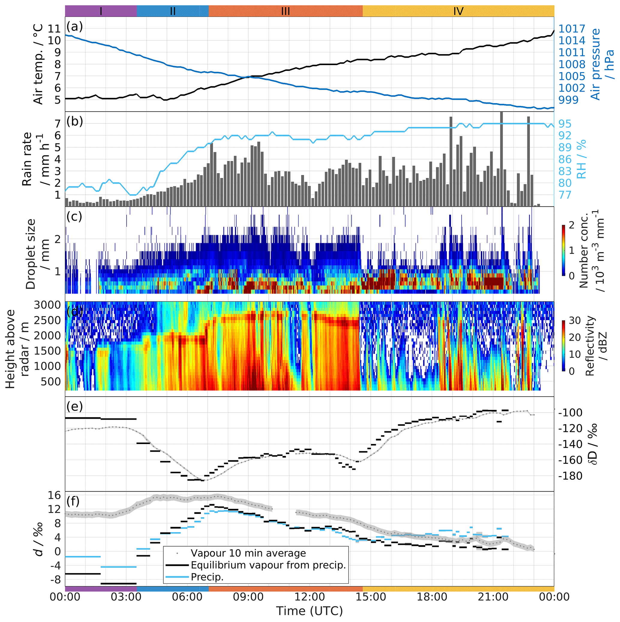
Figure 3 Time series of observations at ∼ 45 m a.s.l. in Bergen between 00:00 UTC 7 December and 00:00 UTC 8 December 2016. (a) Local temperature (black line) and air pressure (blue line) from the automatic weather station (AWS-2700). (b) The 10 min averaged rain rate from the total precipitation sensor (grey shading) and relative humidity from AWS-2700 (blue line). (c) Droplet number concentrations from the Parsivel². (d) The 1 min averaged reflectivity from the micro rain radar. (e) δD of the 10 min averaged vapour (grey dots) and δD of the equilibrium vapour from precipitation (black segments). The uncertainties are 0.60 ‰ and 0.11 ‰ for δD of vapour and the equilibrium vapour from precipitation, respectively. (f) Same as in (e) but for d-excess, including d-excess of precipitation (blue segments). The uncertainty is 0.83 ‰ for d-excess of vapour and 0.20 ‰ for d-excess of the equilibrium vapour from precipitation and precipitation. Precipitation periods I–IV are indicated with colour bars at the top and bottom of the figure.

Precipitation already started forming before the increase in temperature, with rain rates (Fig. 3b, black line) below 1 mm h⁻¹ between 00:00 and 03:30 UTC, and then steadily increasing to 5.5 mm h⁻¹ at 07:00 UTC, varying thereafter at a generally high level with a brief intermission at 12:00 UTC. Rainfall became in particular more variable after 14:30 UTC, reaching brief maxima above 7.0 mm h⁻¹. The total precipitation amount during this 24 h event was 55.3 mm. While measurements from the TPS-3100 are used here, we note that several instruments provide a similar time series of precipitation intensity and comparable precipitation totals (Appendix A).

Relative humidity changed markedly during the event. Before 04:30 UTC, RH varied between 77 % and 80 %. As the precipitation intensified and the temperature started to increase at 05:00 UTC, RH gradually increased to 92 % at 09:00 UTC and remained between 92 % and 95 % thereafter (Fig. 3b, blue line).

The drop size distribution followed a similar evolution as the rain rate (Fig. 3c). At the beginning of the event, raindrop number concentration maxima were small, with the drop size maximum near 0.4 mm (Fig. 4a, Stage I). The drop size spectra started to show a more pronounced peak from 01:30 UTC, as well as an increase in raindrop number concentrations (Fig. 4a, Stage II). On some occasions during Stage II, a bi-modal distribution in drop sizes was observed. Drop size spectra had pronounced maxima at the smallest drop size categories between 09:00 and 11:00 UTC and became broader between 13:00 and 14:30 UTC (Fig. 4a, Stage III). A small number of large raindrops (> 1 mm) had appeared during Stages II and III. The large raindrops had disappeared after entering Stage IV, except for some intense precipitation periods between 18:30 and 20:20 UTC, around 21:30 UTC, and around 22:40 UTC. A particular feature for Stage IV is that the number of large raindrops (0.5–1.0 mm) increases substantially at the expense of raindrops with < 0.5 mm diameter (Fig. 4a, Stage IV). This feature is likely to be associated with the shift from stratiform to convective precipitation.

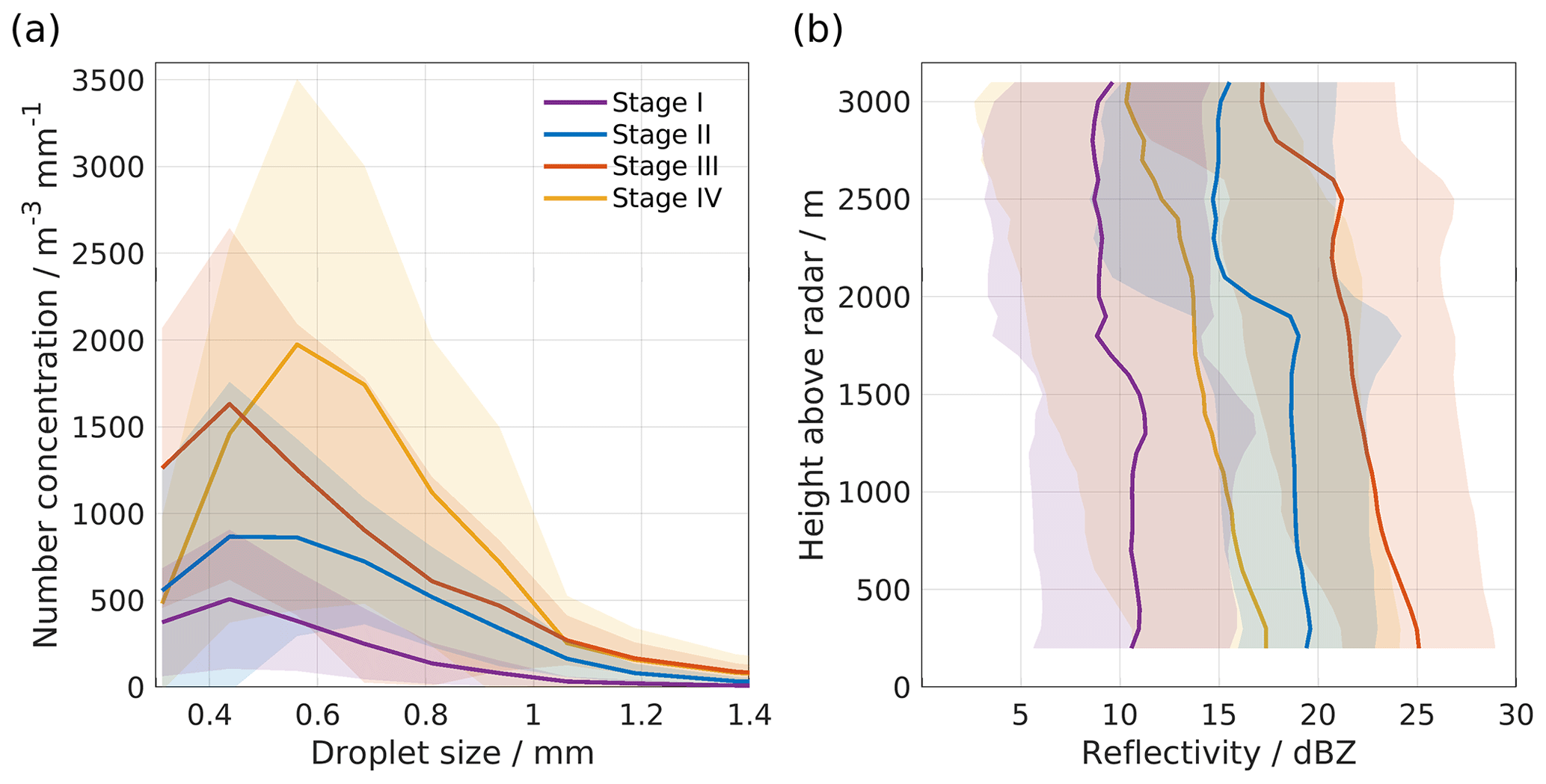
Figure 4 Averaged (a) number concentration of rain droplet per droplet size and (b) reflectivity profile from the micro rain radar at each precipitation stage during the AR event on 7 December 2016. The shading indicates 1 standard deviation. The lowermost layer of the reflectivity profiles has been removed due to ground clutter.

The vertical pointing MRR2 reveals hydrometeor profiles and melting layer height during the event (Fig. 3d). Before 03:30 UTC, precipitation was weak and did not continuously reach the surface, indicating the presence of evaporation of falling hydrometeors, or below-cloud evaporation (Fig. 4b, Stage I). As the precipitation gradually intensified after 03:30, a melting layer started to appear, as well as ice-phase hydrometeors aloft. The melting height increased from 1600 to about 1900 m between 03:30 and 04:30 UTC and increased substantially to 2500 m at 07:00 UTC, thereafter varying between 2500 and 2700 m until 14:30 UTC. The increase in the melting height between Stages II and III is also clearly reflected in the averaged MRR2 profiles (Fig. 4b, Stages II and III). At 07:00 UTC, the second warm front arrives over the measurement location, in close agreement with surface frontal charts and regional weather prediction model forecasts (Fig. 2). Notably, the transition to the second warm front is almost undetectable in surface temperature, precipitation, and relative humidity. During the periods of most intense precipitation (i.e. between 06:30 and 11:20 UTC and between 13:30 and 14:30 UTC), an increase in reflectivity below 500–1500 m indicates droplet growth at low levels (Fig. 4b, Stage III), underlining the importance of water vapour in lower atmospheric layers for the surface precipitation. Almost instantly after 14:30 UTC, there is a change to more intermittent precipitation reflecting the shift from stratiform to a dominantly convective phase of the precipitation event, along with the arrival of the upper-level cold front (Fig. 2c, e). In addition, no more melting layer was detected at this time (Fig. 4b, Stage IV). We speculate that the melting layer vanishes either because the convection was too shallow to reach above the 0 ^∘C isothermal line or because the precipitation was too intermittent to expose a clear melting layer.

3.3 Observed stable isotope signature in vapour and precipitation

The measured isotope composition in the surface vapour and precipitation samples is now compared in relation to the four precipitation stages identified above. For the surface vapour, the 10 min averaged δD_v initially showed a relatively stable value of −120 ‰ at Stage I (Fig. 3e, dotted line). Then δD_v gradually decreased at the start of Stage II (03:30 UTC), until reaching a minimum of −185 ‰ at the end of this stage (07:00 UTC). At Stage III, corresponding to the arrival of the second merged warm front, the value gradually returns to a less depleted level of −160 ‰ at 09:00 UTC and then varies between −160 ‰ and −145 ‰ until 13:30 UTC. As the upper-level cold front arrives, the δD_v first drops to a secondary minimum of −172 ‰, before increasing again during Stage IV (after 14:30 UTC) first rapidly and then more slowly to −110 ‰ around 18:00 UTC and finally −100 ‰ after 21:00 UTC (the least depleted values of the event). The resulting stretched-out “W” shape of the vapour isotope series resembles earlier observations made from high-resolution precipitation sampling (e.g. Muller et al., 2015). The amplitude of 72 ‰ is substantial but smaller than for example observed in rainfall by Coplen et al. (2008). The relative evolution of δ¹⁸O_v closely follows that of δD_v (not shown).

The equilibrium vapour from precipitation δD_p,eq approximately follows the pattern of surface vapour (Fig. 3e, black segments). The isotope signal in surface vapour appears to lag the isotope signal in precipitation by about 30 min. Comparison of specific humidity from the isotope spectrometer with specific humidity calculated from the AWS shows no apparent time lag or offset at 1 min measuring frequency, indicating that atmospheric effects cause this time lag. Overall, the δD_p,eq is more variable than the δD_v time series. At Stage I, δD_p,eq is substantially less depleted than δD_v. This reverses at the beginning of Stage II. During the transition to Stage III, δD_p,eq reaches a minimum, before it again becomes less depleted than δD_v until about 08:30 UTC. Thereafter, differences between δD_v and δD_p,eq are small, with the exception of the last hour of Stage III from 13:30 to 14:30 UTC. The time offset and the relative enrichment and depletion characteristics of vapour and precipitation are further examined in Sect. 4.

The time evolution of the secondary isotope parameter d-excess in surface vapour (d_v) starts with 11 ‰ during Stage I (Fig. 3f, dotted line). Thereafter, d_v increases to 14 ‰ at Stage II and stays around that level until the beginning of Stage III at 08:00 UTC, 1 h after the second warm front arrives. Then d_v gradually decreases throughout the rest of the event, with a more rapid decrease from about 10 ‰ as the upper-level cold front arrives at 14:30 UTC to d_v varying around 4 ‰ between 18:00 and 21:30 UTC and eventually reaching 0 ‰ at 23:00 UTC.

The d-excess of the equilibrium vapour from precipitation (d_p,eq) shows a remarkable difference to d_v at the beginning of the event (Fig. 3f, Stages I and II, black line segments). Here, d_p,eq values are substantially lower than d_v, with the lowest values even being negative (−7 ‰ and −9 ‰) during Stage I. This results in a large difference between d_v and d_p,eq of 18 ‰ and 20 ‰, respectively. During Stage II, d_p,eq gradually approaches d_v, remaining about 2 ‰–4 ‰ lower than d_v. Similar to d_v, d_p,eq then shows a continuous decrease between 07:00 UTC and 16:30 UTC, then stabilizing around 2 ‰. The original d-excess of precipitation, d_p (Fig. 3f, blue line segments), should theoretically be equal to d_p,eq. Small discrepancies at Stage I, Stage IV, and the two depletion minima may at least partly arise from the definition of the d-excess (Dütsch et al., 2017).

As is evident from the results presented above, the precipitation and vapour isotope measurements, especially when combining δD and d-excess parameters, clearly provide signals that are not apparent in standard meteorological observations, such as air temperature and rain rate. Following our hypothesis that the isotope signature at each stage reflects the impact of several atmospheric processes, including moisture origin, processes during advection and mixing, condensation processes in clouds, and below-cloud interaction, we now attempt to disentangle the individual contributions from these processes on the observed isotope signature at the surface during the AR event.

4 Impacts on the stable water isotope signature

The precipitation isotope signal during a weather event results from a convolution of different processes. We now proceed backwards from the last process, the below-cloud interaction, to weather system and transport influences and to the moisture source signal to investigate how different processes contribute throughout the event.

4.1 Contribution from below-cloud interaction processes

Microphysical processes within clouds and post-condensational exchange processes of falling precipitation can alter the isotope composition. While isotopic equilibrium can be assumed for rain formation in warm clouds, kinetic effect exists at snow formation. Vapour deposition in a supersaturated environment with respect to ice, therefore, increases d-excess in precipitation (Jouzel and Merlivat, 1984). Liotta et al. (2006) proposed that higher d-excess also exists in orographic clouds since kinetic effects should be expected in the first step of droplet formation, when in-cloud droplets are short-lived and thus can not reach equilibrium with the surrounding vapour. For deep convective systems, factors such as condensate lifting, convective detrainment, and evaporation in unsaturated downdrafts can play a critical role in the control of the isotope composition of precipitation (Bony et al., 2008).

Below-cloud interaction processes consist of the continuous exchange of falling precipitation with the surrounding vapour in the atmospheric column below cloud base (Miyake et al., 1968; Barras and Simmonds, 2009; Guan et al., 2013; Wang et al., 2016). In undersaturated conditions, the vapour exchange will lead to a net mass loss of the droplets. Therefore, below-cloud evaporation usually dominates at the beginning of a precipitation event, when the atmosphere below cloud base is still unsaturated. In near-saturated conditions, liquid precipitation will exchange with surrounding vapour in a near-equilibrium process. Resulting from the same underlying process, both exchanges are strongly influenced by drop size, whereby smaller droplets are affected more strongly (Graf, 2017). Depending on the intensity of below-cloud exchange processes, the isotope composition of precipitation can deviate more or less strongly from Rayleigh model expectations.

We investigate the change in isotope composition due to below-cloud processes using the ΔδΔd diagram (Graf et al., 2019). The ΔδΔd diagram uses the differences between equilibrium vapour from precipitation and ambient vapour in terms of both δD and d-excess (Δδ and Δd, Sect. 2.5) as its axes (Fig. 5). The diagram is divided by the zero reference lines into four quadrants. The closer data points are located near the origin, the closer the equilibrium between the vapour and liquid precipitation. Data points located in the lower right quadrant have positive Δδ and negative Δd values, reflecting the impact of strong evaporation below cloud base. Conversely, data points in the lower-left quadrant have undergone moderate below-cloud evaporation and equilibration. Negative Δδ values indicate that the (more depleted) isotope signal from the cloud level is preserved in precipitation and has not been overprinted by below-cloud equilibration. In other words, below-cloud equilibration is incomplete in these cases.

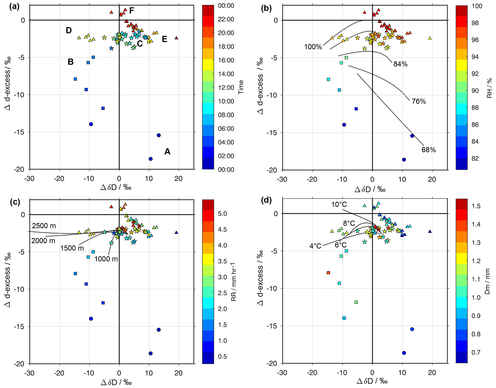
Figure 5 ΔδΔd diagram for precipitation samples collected during the AR event on 7 December 2016. Samples coloured according to (a) sampling start time (UTC), (b) relative humidity at the surface (RH, %), (c) rain rate (RR, mm h⁻¹), and (d) droplet mean diameter (D_m, mm). Letters in panel (a) mark time periods (see text for details). Grey lines in panels (b–d) show sensitivity experiments with the idealized below-cloud interaction model of Graf et al. (2019) regarding the parameters surface air temperature (T_a), cloud base height (z_c), and relative humidity at the surface with regard to a reference simulation. Thereby, each line represents a range of drop sizes (see Appendix B for details). Circles: Stage I; squares: Stage II; stars: Stage III; triangles: Stage IV.

The temporal evolution of the precipitation samples during the AR event proceeds from the lower right quadrant, with the first to samples from Stage I displaying the strongest influence of below-cloud evaporation (Fig. 5a, letter A, circles). Samples from Stage II are in the bottom left quadrant, first reflecting moderate below-cloud evaporation and some equilibration (letter B, squares). Towards Stage III (08:30 UTC), samples are close to equilibrium with surface vapour, with slightly negative Δd values (0 ‰ to −4 ‰) and a relatively large spread of both positive and negative ΔδD values (12 ‰ to −12 ‰, letter C, stars). An interesting phenomenon then occurs at the transition to Stage IV, when first a stronger cloud influence is apparent, with data points near −10 ‰ for Δδ (Fig. 5a, letter D, triangles), before directly jumping to +10 ‰ after 15:00 UTC (Fig. 5a, letter E). For the remainder of Stage IV, data points then progressively move closer to equilibrium conditions, corresponding to the origin of the coordinate axes (letter F). Note that the samples from different stages are well separated in the diagram, indicating different dominating processes at each stage.

A key factor of influence for the below-cloud evaporation is RH below cloud base. When coloured by RH from the AWS, it is evident that the samples most affected by below-cloud evaporation coincide with below 90 % RH at the surface (Fig. 5b). The precipitation samples remain at non-equilibrium at 90 % RH–95 % RH and reach the origin only for above 95 % RH. A sensitivity study with idealized simulations using BCIM (below-cloud interaction model; Graf et al., 2019) using different drop sizes and values of RH provides lines that indicate drop-size-dependent effects of RH on raindrops falling from 1500 m to the surface. Thereby, initial conditions approximately resemble the situation during Stages I and II. Here we use lines representing a range of drop sizes for a specific parameter value similar to a coordinate system (for details see Appendix B). Albeit offset by about 10 %–15 % from observed RH, the sensitivity study shows a clear tendency towards lower Δd with lower below-cloud RH.

While RH is a key driver of below-cloud interaction, several other factors are also important, such as rain rate. The two samples with the lowest rain rates of about 0.5 mm h⁻¹ (during Stage I) are located in the lower right quadrant of the ΔδΔd diagram (Fig. 5c). Several subsequent samples with slightly higher rain rate (∼ 0.9–2.2 mm h⁻¹) are located in the left quadrant, ranging from about −15 ‰ to −6 ‰ in Δd. As the rain rate of the sample further increases and the ambient air nearly saturates, the effect from below-cloud evaporation weakens. Samples with relatively heavy rain rates (mostly between 3 and 5 mm h⁻¹) are found during the rest period of the event; they are located close to the zero Δd line, indicating weak influences from below-cloud interactions. A sensitivity analysis of the formation height parameter in the BCIM model shows weak sensitivity that aligns horizontally along the Δδ axis with increasing height. Interestingly, this agrees with data points at the transition to Stage III when the melting layer was among the highest (Fig. 3d).

The small rain rates are also a consequence of the below-cloud evaporation in an undersaturated environment. This below-cloud evaporation also leads to a reduced size of precipitation droplets, characterized by the droplet mean diameter. In the ΔδΔd diagram, the samples with the lowest rain rates also have a small droplet mean diameter of below 0.9 mm (Fig. 5d). There are further samples with mean diameters below 1 mm during Stage IV of the precipitation event. At these times, rather than being due to evaporation effects, the small drop sizes and the near-saturation conditions indicate that droplet growth may be taking place actively. An analysis of the sensitivity to the temperature profile with the BCIM shows a sloping of the sensitivity from a horizontal to a diagonal orientation with warmer temperatures. This is in qualitative agreement with the observations during the event with surface warming continuing from Stage III through Stage IV. Overall, Δd appears more readily explained by RH, rain rate, and drop size. A possible reason is that we did not modify the background vapour profiles, which can have a strong influence on Δδ.

In summary, we observe strong below-cloud interaction at the beginning of the rainfall event. The period (Stages I and II) is characterized by the least saturated ambient air, the lowest rain rate, the smallest droplet size, and the lowest melting layer height. All these features except the melting layer height favour the occurrence of the below-cloud evaporation. Transition phases between the stages increase the disequilibrium between surface vapour and precipitation, with the precipitation signal leading the vapour in characteristic ways (Fig. 5a, letters A–F). The non-equilibrium fractionation during the evaporation causes the rain droplets to be less depleted in heavy isotopes (i.e. higher δ¹⁸O and δD values). At the same time, due to non-equilibrium conditions, relatively more HD¹⁶O than H${}_{\mathrm{2}}^{\mathrm{18}}$O will leave the droplet, yielding to a low or even negative d-excess in the remaining rain droplet. These isotope signatures match the precipitation samples taken during this period (Figs. 3e, f, 5). The variation during Stage III and IV, however, shows that these two stages are less affected by below-cloud interactions and more related to a change in parameters related to the weather system, such as formation height and the temperature profiles. We, therefore, focus now on the potential contribution of weather-system-related changes to the isotope composition of surface vapour and precipitation during the AR event.

4.2 Weather system contribution

We now use the four stages, defined based on the surface meteorological observations (Fig. 3), to investigate the relationship between the observed isotope signatures and weather system characteristics.

During atmospheric transport, water vapour is depleted in heavy isotopes due to an atmospheric distillation process (Jouzel et al., 2007). The rainout history during the transport essentially depends on the temperature difference between the moisture source and the condensation height above the precipitation site. This has been historically known as the rainout effect and can be approximated as a Rayleigh distillation process (Dansgaard, 1964). A larger temperature difference leads to a greater rainout process and thus a more depleted isotope profile in the condensate, which ultimately translates to precipitation. For example, Dansgaard (1953) explained the gradual enrichment of ¹⁸O abundance in the precipitation from a warm front with the decreasing condensation temperature as the front passes the observation site.

In comparison to such idealized transport concepts, the AR event studied here is substantially more complex. As apparent from the gradients in air temperature at 850 hPa around 06:00 UTC (Fig. 2c), the AR is composed of two staggered warm fronts passing over Bergen in close sequence (Sect. 3). A more continuous display of the frontal passage is provided by a time–height cross section of equivalent potential temperature (θ_e), cloud water, and precipitation, using hourly ERA5 reanalysis data (Fig. 6). We now attempt to identify periods where the surface isotope measurements can be considered as representative for the air mass overhead.

The cross section depicts a constantly increasing temperature (shading) on the surface (below 850 hPa), consistent with the surface meteorological observations, as well as a descending cloud base (black dotted line). A relatively deep layer of cold air near the surface present at the beginning of Stage I is replaced by warmer and more humid air. The cloud base is initially near 850 hPa, as seen by the gradient in cloud water, just below the melting layer, which is at about 830 hPa at this time (purple solid line). Towards Stage II, there is an increasing contribution of ice-phase processes to the surface precipitation, with cloud ice of above 0.15 g kg⁻¹ near 450 hPa (white dotted lines). Snowfall rates increase from 0.1 to above 0.4 mm h⁻¹ above the melting layer (white solid line), indicating riming of the ice particles between 600–750 hPa as an important contribution to the precipitation. The adequacy of this overall sequence is supported by the MRR2 radar observations (Fig. 3d) but indicates a delay of about 2–3 h in the ERA5 dataset.

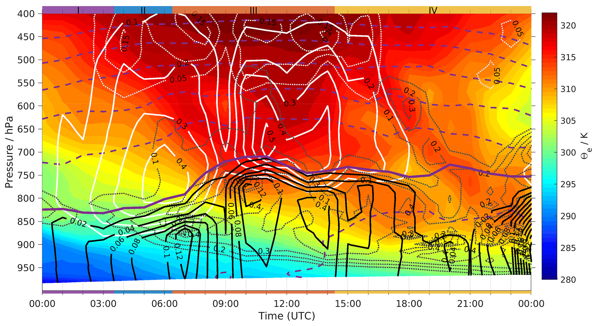
Figure 6 Hourly equivalent potential temperature from ERA5 reanalysis for the observation site at Bergen between 00:00 UTC 7 December and 00:00 UTC 8 December 2016. The solid white line indicates specific snow water content and the dotted white line specific cloud ice water content. The solid black line indicates specific rain water content and the dotted black line specific cloud liquid water content. The unit of all contours for different water species is g kg⁻¹. The thick purple line indicates the 0 ^∘C isothermal line, and dashed purple lines indicate isothermal lines deviating from the 0 ^∘C isothermal line with 5 ^∘C intervals. Colour bars at the top and bottom indicate precipitation periods I–IV.

The isotope compositions of surface vapour and precipitation during Stages I and II are initially dominated by below-cloud interaction. Both surface vapour and equilibrium vapour from precipitation exhibited less depleted δD (Fig. 3e), although probably for different reasons. With the isotope signal in the precipitation leading that in the vapour, the weather system signal progressively becomes more dominant throughout Stage II, levelling at −180 ‰ between 05:00 and 06:00 UTC. We consider this the actual δD isotope signature of the first frontal air mass.

The increase in d-excess of surface vapour from 12 ‰ to 15 ‰ from Stage I to Stage II could reflect a gradual shift from the pre-frontal to the newly arriving warm-frontal air mass. However, the large distance between the d-excess of equilibrium vapour from precipitation from surface vapour indicates the influence of the below-cloud evaporation. The converging d-excess of equilibrium vapour from precipitation and d-excess of surface vapour at the end of Stage II indicates a balance between column vapour and precipitation. We therefore consider ∼ 14 ‰ as the most likely value for d-excess signal of the first warm front.

The transition to Stage III with the second warm front is indicated by a substantial jump in melting layer height to 700 hPa around 07:00–08:00 UTC (Fig. 6, purple line) and a gap in snowfall and intensified precipitation around 09:00 UTC. At this time, the cloud becomes markedly deeper, and regions of cloud liquid and cloud ice overlap at 550 hPa. Precipitation shows a maximum above 800 hPa and decreases below. This rain evaporation may be overestimated by the reanalysis since the precipitation radar instead shows an increase in reflectivity in the lowest 1000 m above the surface (Fig. 3d). The isotope signal of this second warm front is less depleted and produces a transition to about −160 ‰ for δD, led by the precipitation (Fig. 3e). The plateau in δD reached after about 09:00 UTC indicates that this likely is the actual isotope signal of the second warm front. The d-excess of both surface vapour and equilibrium vapour from precipitation during Stage III gradually decreased from 15 ‰ to 9 ‰ for the vapour and from 13 ‰ to 6 ‰ for precipitation. A plateau reached in the precipitation d-excess after 11:00 UTC indicates that the steady state in below-cloud exchange has been reached; thus the signal of the air mass likely dominates surface observations at this time.

In addition to being warmer, cloud processes extend over a deeper section of the lower and middle troposphere during the second front. The enriching trend probably corresponds to a gradual lowering of the effective condensation level. The lowering here appears connected to the lowering of the cloud base height, allowing an increased contribution to falling raindrops that gain mass from, for example, the collision with droplets formed at low levels. Indeed, we observe a noticeable increase in radar reflectivity at the surface level below 1500 m during Stage III (Figs. 3d and 4b). The contribution of low-level vapour to surface precipitation is also consistent with the arguments by Yoshimura et al. (2010) based on a regional model study of an AR event that the precipitation isotope signal can be influenced by a deep section of the atmosphere.

In the ERA5 reanalysis, the middle and lower troposphere starts to become more unstable after 14:00 UTC, as indicated by θ_e changing from about 320 K to about 305 K towards the end of the day. Noting the shift by 3 h in relation to observations, the transition to Stage IV is marked by the disappearance of ice-phase precipitation, with a tongue of cloud water reaching above 600 hPa and cold air overrunning the warm front at about 720 hPa at 18:00 UTC (Fig. 2b). The very intense precipitation lasting for a 1 h period at the end of Stage III, associated with strong deviations in the ΔδΔd diagram, could be related to moist convection forming at this thermodynamic instability. The local δD minimum of −175 ‰ at the transition of Stage III to Stage IV would then represent a higher-elevation cloud signal, reflecting the isotope gradients in the column.

The stable stratification weakens further during the remainder of Stage IV, leading to a change from stratiform to convective precipitation. Precipitation formation shifts to the lower troposphere, mostly below the melting layer height, consistent with MRR2 measurements (Fig. 3d). The apparent lack of a melting layer implies condensation temperatures above 0 ^∘C. The δD of both surface vapour and equilibrium vapour from precipitation gradually becomes less depleted, reaching −110 ‰ around 18:00 UTC and finally −100 ‰ after 21:00 UTC, even less depleted compared with the values during Stage I (Fig. 3e). The increased δD values reflect the shift to precipitation formation dominated by low-level water vapour, consistent with earlier studies (Lowenthal et al., 2011). The d-excess plateaus at about 4 ‰ after about 16:00 UTC, with the equilibrium vapour trending towards 0 ‰ towards the end of the event. With the cloud water isolines nearing the surface, and near-saturated conditions in observations, the isotope signal essentially reflects conditions within a condensing air mass.

In order to assess whether a Rayleigh model is capable of diagnosing condensation temperatures and condensation heights during the different stages of the AR event, we apply the Rayleigh fractionation model of Jouzel and Merlivat (1984). Hereby, the condensation temperature of the precipitation is obtained when the modelled δD from a moist adiabatic ascent became equivalent to the observed δD in surface precipitation (Table 1). The modelled condensation height of Stage I is 1280 m. With 14.1 ^∘C, the condensation temperature is substantially higher than the measured surface temperature of ∼ 5 ^∘C. At Stage II, the modelled condensation temperature decreases to 0.9 ^∘C, and condensation height increases to 3900 m. In Stage III, the modelled condensation temperature increases to 2.4 ^∘C, corresponding to a condensation height of 3600 m. At Stage IV, the modelled condensation temperature increases to 13.6 ^∘C, and condensation height becomes 1390 m. The overestimation of condensation temperature at least partly reflects the sensitivity of such estimates to initial temperature conditions. The overall low d-excess from the Rayleigh model calculations may be associated with the high sensitivity of d-excess on the representation of supersaturation conditions during ice formation in cloud (Jouzel and Merlivat, 1984).

Throughout the event, it is apparent that the condensation heights estimated from the Rayleigh model are substantially lower than cloud top heights reaching above 5500 m (∼ 500 hPa, Fig. 6). In fact, according to ERA5, cloud top temperatures reach below −25 ^∘C. Consistent with MRR2 observations, the relatively warm condensation temperatures during the stratiform phase compared to cloud-top conditions indicate that lower atmospheric layers contribute substantially to the precipitation total. For the two most depleted δD periods, condensation temperatures are −4.1 and −2.3 ^∘C. Also in these two most depleted situations, the condensation temperature from the Rayleigh model is more consistent with a mass-weighted average of condensation, rather than cloud-top temperatures, indicating the limitation of Rayleigh models in diagnosing condensation conditions within stratiform clouds.

We now proceed to explore to what extent the isotope signals of the different air masses during Stages II to IV reflect the moisture source and transport conditions.

Table 1 The observed rain rate (RR) and isotope compositions (δD, d-excess) and the corresponding model estimate of condensation temperature (T_c), condensation height (Z_c), and d-excess of the surface precipitation (d_c) during the AR event on 7 December 2016 in Bergen. The model estimates are calculated using the observed δD values of the surface precipitation, according to a Rayleigh fractionation model of Jouzel and Merlivat (1984). Supersaturation over ice S_i is assumed to occur during ice formation and is represented with a linear formula S_i =1−0.004T (T in ^∘C) after Risi et al. (2010). Input conditions have been taken from global average conditions according to Craig and Gordon (1965) as T₀ = 20 ^∘C, RH₀ = 0.75, δ¹⁸O₀ =-13 ‰, and δD₀ =−94 ‰.

4.3 Relation of moisture sources to meteorological evolution

We now focus on how moisture sources and moisture transport to Bergen are connected to the weather system configuration and thus potentially contribute to the isotope signal in water vapour and precipitation.

Ocean–atmosphere conditions at the moisture source affect the isotope composition of generated water vapour (Gat, 1996). Theoretical studies and observations have shown that d-excess in the generated vapour over ocean surface is dependent on relative humidity (RH) with respect to sea surface temperature (SST) and to second order to the SST itself in the source area (Merlivat and Jouzel, 1979; Uemura et al., 2008; Pfahl and Sodemann, 2014). As an example, high d-excess anomalies are usually observed in water vapour formed during so-called marine cold air outbreaks (Aemisegger and Sjolte, 2018; Aemisegger, 2018), where cold dry air moves over relatively warm ocean waters and triggers strong evaporation (Papritz and Spengler, 2017; Papritz and Sodemann, 2018). In contrast, land regions and more calm ocean evaporation are associated with lower d-excess (Aemisegger et al., 2014; Thurnherr et al., 2020). The d-excess is often assumed to be conserved during transport. However, microphysical processes within and below clouds can influence the d-excess in local precipitation and thus obscure information on the evaporation conditions in the source area (Jouzel and Merlivat, 1984; Graf et al., 2019).

In this context, we now return to the synoptic development over the 3 d proceeding the precipitation event and the location of the moisture sources and corresponding evaporation conditions. On 4 December 2016, two low-pressure systems are located south of Greenland and in the North Atlantic. Strong moisture transport takes place at the southern flank in the warm sector region, displayed as IVT above 800 kg (ms)⁻¹ (Fig. 7a). Bergen (red cross) is under the influence of a weak pressure gradient, with an onshore flow from NE and lower humidity. Moisture uptakes contributing to precipitation in Bergen during the AR event are identified for the respective time periods. The most substantial moisture uptake (thick blue-green contours) contributing to the precipitation on 7 December 2016 coincides with the location of the AR.

Figure 7 Synoptic situation at 12:00 UTC on the 3 d prior to the AR event day (a–c) and on 7 December 2016 (d). Shown are integrated water vapour transport (IVT > 250 kg (ms)⁻¹, shading), mean sea level pressure (black contours, 5 hPa interval), and concurrent moisture uptake (mm (6 h)⁻¹, blue-green contours) that precipitates at the arrival location at 00:00 UTC between 7 and 8 December 2016. The red cross indicates the measurement site Bergen, Norway.

On 5 December, the two low-pressure systems have merged, with a core low below 975 hPa near Iceland (Fig. 7b). IVT in the frontal band has intensified. In southern Norway and central Europe, high pressure is starting to form, with a 1030 hPa core pressure. The moisture uptake has moved further north and overlaps now with the IVT maximum. This warm frontal band coincides with the two warm fronts passing southern Norway during the event (Fig. 2a). On 6 December at 12:00 UTC, the cyclone had entirely separated from its frontal bands and started to fill in. High pressure over Europe increased to 1040 hPa, with the pressure gradient further accelerating the onshore flow, supporting an intense meridional IVT of above 800 kg (ms)⁻¹. Moisture sources advanced substantially further to the northeast, with the IVT maximum concentrated south of the British Isles. On 7 December, a small, secondary cyclone dominated the moisture flux in the north, while the southern part of the IVT structure remained supported by yet another low-pressure system downstream (Fig. 7d). Moisture uptakes are identified over the North Sea near Scotland (blue-green contours), contributing to precipitation in Bergen later that day. The area over Scotland corresponded to relatively cold air with broken clouds intruding at the rear side, over the UK, belonging to the cold frontal air during Stage IV (not shown).

In summary, moisture transport and moisture uptakes were clearly connected to the frontal structures during the AR event. The most substantial moisture uptake was occurring in the vicinity of the IVT maximum, embedded in the fused warm frontal bands. As the time window to the precipitation event shortened, the moisture uptake moved substantially further northward over the North Sea. This change in moisture source distance corresponds at least qualitatively to the progressively less depleted isotope signature during the event. We now investigate more quantitatively how different the evaporation conditions at the moisture sources were for Stages II, III, and IV.

4.3.1 Moisture source contribution

The evaporation conditions at the moisture sources identified above determine the vapour isotope composition before the start of the condensation processes. Here we investigate whether the stepwise decrease in precipitation d-excess observed during Stage II and Stage III can be related to changes in moisture source conditions. Moisture source conditions are quantified here in terms of moisture source distance, surface temperature, and relative humidity with respect to sea surface temperature (Fig. 8a–c).

Figure 8 Histograms of moisture source conditions identified with the Lagrangian moisture source diagnostics from 20 d backward trajectories during the AR event in southwestern Norway. (a) Moisture source distance (km), (b) moisture source temperature (^∘C), (c) moisture source relative humidity with respect to sea surface temperature (RH_SST), and (d) d-excess estimated from the empirical relation of Pfahl and Sodemann (2014). Grey filled bars show the most intense period of the event (Phase III, 07 December 2016 at 12:00 UTC), dotted lines the 12 h before (Stage I and II), and solid lines the 12 h after the central period (Stage IV). Histograms represent the normalized contributions of each moisture source location to the precipitation at the arrival region on the respective date. The star symbol indicates the mean value of the distribution at 12:00 UTC on 7 December 2016.

The large majority of moisture uptakes took place within a distance of 8000 km (Fig. 8a). The histogram for the main precipitation event at 12:00 UTC on 7 December 2016 is shown as grey shading, while the preceding time steps are shown as dashed lines, and the later ones are shown as solid lines. During the sequence of the event, moisture sources shifted from local sources (less than 1000 km distance at 00:00 UTC on 7 December 2016) to the most distant at 12:00 UTC and finally again to closer locations (3000–4000 km distance), with a combination of local and remote sources at 00:00 UTC on 8 December 2016. An analysis of the corresponding moisture lifetime (not shown) provides the shortest lifetimes during the main precipitation phase at 12:00 UTC, with a median of about 3 d. This timing corresponds to uptake locations from 4 to 7 December 2016 as shown in Fig. 7. In earlier and later stages, lifetime distributions also peak at less than 5 d, while including more notable contributions with more than 5 d since evaporation.

Along with the shift in the moisture source location, evaporation conditions also changed. The most frequent temperature at the moisture sources was about 23 ^∘C throughout the event, yet including a range of colder temperature conditions (Fig. 8b). Colder temperatures contributed in particular during the beginning of the event, when the average moisture source temperature was 17.6 ^∘C at 00:00 UTC on 7 December 2016 (purple dashed line), clearly cooler than the mean of 19.7 ^∘C at 12:00 UTC (star symbol), and moisture sources were more local. Overall, the range of moisture source temperature variations was relatively limited throughout the event (within 2 ^∘C).

The relative humidity with respect to the SST (RH_SST) is a key factor in kinetic fractionation during evaporation (Craig and Gordon, 1965). Throughout the event, the mean RH_SST is around 65 %–70 % (Fig. 8c, star symbol). The peak at near 100 % is an artefact of the contribution from land regions where RH_SST is not defined. The maximum RH_SST shifts during the event, from above 60 % before the most intense precipitation period to 55 % at 12:00 UTC on 7 December 2016. It appears that the most intense precipitation stage was thus also associated with the most intense evaporation due to the strongest humidity gradient over the North Atlantic moisture sources.

For comparison with the stable isotope measurements, we predict the d-excess at the moisture source from the empirical relation between RH_SST and d-excess by Pfahl and Sodemann (2014) (Fig. 8d). The highest d-excess from the moisture sources is predicted during the peak of the precipitation event, with a maximum at 16 ‰ (grey shading). As for RH_SST, land sources produce an artefact for d-excess below −5 ‰. Both before and after the main precipitation period, the maximum in the d-excess distribution is shifted to lower values. This sequence from low to high to low d-excess throughout the event is qualitatively consistent with the observed d-excess signal. The initial low and even negative d-excess in precipitation during Stage I is thus likely a combination of the moisture source conditions, amplified by below-cloud evaporation. The source d-excess is more sensitive to RH_SST than to SST (Merlivat and Jouzel, 1979; Aemisegger et al., 2014). Additionally, considering that the source temperatures only change slightly during the event, the humidity gradient above the moisture sources appears as the dominant driver of the d-excess changes observed here.

Considering a longer time period around the case investigated here, the Lagrangian diagnostic indicates a rather constant d-excess value during the whole precipitation event (Fig. C1d). The observed d-excess variation is not captured by the Lagrangian diagnostic. The detailed inspection of Fig. 8 indicates the lack of variability is likely due to averaging the complex histograms to one value at the arrival location. The key characteristic of the histogram distribution is the maximum probability, but skewed and bimodal distributions make it difficult to provide more robust statistic measures. To represent the full variability of the moisture source conditions, detailed inspection of the moisture source properties throughout the event is therefore needed.

5 Discussion

We now return to the initially mentioned dispute in the literature regarding the interpretation of the precipitation isotope signal from an AR case making landfall at the coast of California. From sampling precipitation at a 30 min time interval during the AR event, Coplen et al. (2008) found a remarkable variation in δD of 60 ‰, progressing from less depleted to depleted and back. Both the shape and amplitude of the stable isotope variation were similar to the case studied here. Coplen et al. (2008) based the interpretation of the variability primarily on changes in cloud height, i.e. the temperature of condensation (Scholl et al., 2007). Using a Rayleigh distillation model, it was proposed that the depleted phase would correspond to clouds with an average T_c of −4.2 ^∘C (Coplen et al., 2008).

Yoshimura et al. (2010) then simulated the same AR event with a regional isotope-enabled model, leading them to propose a fundamentally different explanation for the isotope variation in surface precipitation observed by Coplen et al. (2008). According to that interpretation, the less depleted isotope composition of precipitation at the beginning of the event would be caused by below-cloud evaporation. Furthermore, Yoshimura et al. (2010) found from their simulation that up to one-third of the condensate would be contributed from the lower troposphere (below 800 hPa), with an increasing tendency throughout the event. Notably, the contribution from the cloud top would decrease during the most depleted phase of the event. Despite uncertainties in some model parameters and parameterizations, Yoshimura et al. (2010) concluded from their analysis that cloud microphysics, below-cloud exchange, and advection all play a role in the observed isotope variation during different phases of the event.

Expanding the dataset to 43 events sampled with a network of automatic rain samplers across northern California, Coplen et al. (2015) confirmed the pronounced isotope variation during events as discussed in Coplen et al. (2008). Further, they argued that if the below-cloud evaporation were to explain the initial low depletion as proposed by Yoshimura et al. (2010), kinetic effects due to evaporation should have led to characteristic deviations from the global meteoric water line.

The above controversy revolves around two questions. (i) What is the contribution from below-cloud interaction, and in particular evaporation, to the precipitation isotope signal? (ii) Are Rayleigh-type models adequate to explain the surface precipitation signal during AR cases? Based on our highly detailed analysis of an AR event, with high-resolution precipitation sampling and simultaneous water vapour measurements, we are in a situation to contribute constructively to both aspects of this scientific controversy.

5.1 Contribution from below-cloud interaction to the isotope composition in surface precipitation

The joint observation of both surface vapour and precipitation in this study shows a characteristic time lag of the vapour over the precipitation signal. One plausible explanation for this time lag is that diffusional interaction takes place between precipitation and the surrounding vapour over extended time periods. Even though the total column mass of precipitation in a column is typically only about $\mathrm{1}/\mathrm{10}$th of the IWV, precipitation persisting over longer periods will imprint on ambient vapour isotope composition, and vice versa. As more precipitation falls, the below-cloud air gradually saturates, reducing the vertical isotope gradient and eventually reaching isotopic equilibrium with the precipitation. At that point, the time lag between precipitation and vapour isotopes would vanish. Here, we find this time lag to be on the order of 30 min.

As long as the surface air is unsaturated, net mass transfer is directed away from raindrops; thus below-cloud evaporation reduces drop sizes and rainfall amounts, causing characteristic deviations in the ΔδΔd framework that reflect kinetic fractionation effects (Fig. 5). The rainfall contributed during Stage I in this study was, however, too small to markedly influence the isotope composition of the rainfall total (Table 1). Concerning the scientific controversy introduced above, we note that below-cloud processes can influence precipitation and surface vapour, but the signal can be too small to detect whether sampling interval is too long or due to sampling and analytical uncertainty. It is therefore not possible to confirm that the initial low depletion in the dataset of Coplen et al. (2008) was actually due to below-cloud evaporation, in particular without additional vapour measurements. Other factors, such as advection or progressive vapour–precipitation exchange, could also have contributed to the initial low depletion.

5.2 Adequacy of the Rayleigh model to explain the isotope composition in surface precipitation

The majority of the precipitation in ARs is arriving with the strong onshore flow of the warm sector, led by the warm front and dominated by long-range transport. Large-scale ascent, enforced by orographic lifting and condensation heating during landfall, leads to condensation and predominantly stratiform cloud formation. The warm conveyor belt (WCB) model is often used to describe the strongest precipitation-generating airflow in the warm sector of cyclones (Madonna, 2013). According to a common classification criterion, air masses in the WCB airstream rise 300 hPa or more in 48 h, corresponding to vertical ascent on the order of several centimetres per second. Precipitation from cold-sector air masses, in contrast, has a more convective nature, characterized by an isolated ascent in updrafts and dominated by vertical motions on the order of up to several metres per second.

From the Rayleigh model simulation presented in Sect. 4.2, we find that the condensation temperature of the surface precipitation is most consistent with the temperature profiles in the reanalysis data (Fig. 6, purple contours) when interpreted as a representation of the vapour-mass-weighted average in the column rather than the cloud base or cloud top temperatures. MRR2 reflectivity profiles for the four precipitation stages confirm that lower levels contribute substantially to the surface precipitation.

Variants of the Rayleigh distillation model are often used to represent the isotope fractionation during condensation processes (e.g. Jouzel and Merlivat, 1984). However, precipitation entering from above into air parcels, as well as the isotopic exchange of the falling precipitation with vapour inside the air parcel, is not part of Rayleigh distillation models. Rayleigh models may thus only be adequate to simulate the vapour composition in a rising air parcel and the precipitation falling directly from it, corresponding to isolated convective clouds. For slowly ascending warm-sector air masses, where clouds contribute to condensation at a range of atmospheric layers, a single air parcel appears insufficient to capture the actual precipitation process. Conceptually, one could instead consider an entire stack of air parcels, each represented by a Rayleigh model, as a more adequate representation of stratiform clouds (e.g. Rozanski and Sonntag, 1982). Each air parcel in the column is at or near saturation, contains cloud droplets, and will receive input of hydrometeors from above and thus contributes to the precipitation by condensation or deposition, riming, scavenging, and partially equilibrating with the water vapour while passing through. The vertical connection of an entire stack of Rayleigh-type parcels would create a more efficient coupled fractionation process than an isolated Rayleigh model. In light of such a vertically coupled “Rayleigh stack”, a single cloud top or condensation temperature from one Rayleigh model appears too limited to capture the influences on the fractionation process in the entire cloud. This is underlined by the fact that in Coplen et al. (2008) the Rayleigh model only needed temperatures down to −4.2 ^∘C to explain the observed precipitation isotopes, which could not be reconciled by the range of temperatures throughout the entire column found by Yoshimura et al. (2010). A similar observation was made here with the Rayleigh model of Jouzel and Merlivat (1984).

As the precipitating warm-frontal air mass is advected horizontally with the AR, it will produce a coherent isotope signal at the surface, as noted by the displacement times (Coplen et al., 2015). Coplen et al. (2015) also noted that there is no immediate relation between the isotopic depletion and either the total amount or the intensity of precipitation during landfall. Both of these findings are consistent with the interpretation that the isotope composition of the stratiform cloud can obtain a coherent, depleted isotope signature from a sustained lifting process. The isotope signal of stratiform cloud then reflects a time-integrated condensation history of the air masses, whereas surface precipitation is a combination of the air mass signature, the surface vapour, and the below-cloud interaction processes.

We conclude from this discussion that since the isotope signal in precipitation is intimately coupled to the cloud microphysics and dynamics, the Rayleigh perspective can only be adequate to represent the isotope composition near cloud top and in some convective situations. For surface precipitation, and precipitation from deep stratiform clouds in frontal systems such as ARs, the Rayleigh model reaches conceptual limitations. Despite their own uncertainties, it, therefore, appears necessary to invoke more complex numerical tools in the interpretation, such as isotope-enabled numerical weather prediction models, or Rayleigh-type models adapted to stratiform clouds.

6 Conclusions and further remarks

We have presented the high-resolution stable isotope signature of a land-falling atmospheric river in southwestern Norway during winter 2016. Figure 9 provides a conceptual summary of the sequence of events, by providing a spatial depiction of the air masses arriving at Bergen. In surface precipitation, we observe δD that develops in a stretched “W” shape (between −180 and −100 ‰ for equilibrium vapour of precipitation) and d-excess that increases from −9 ‰ to 13 ‰, followed by a gradual decrease to 0 ‰. In surface vapour, δD exhibits the same “W” shape, following closely to the precipitation isotope variation, with a lag of about 30 min. The d-excess in vapour, increasing from 10 ‰ to 16 ‰, differs markedly from the d-excess in precipitation in the beginning. As the relative humidity below cloud base increases, the vapour d-excess follows the same trend as that of the precipitation, reaching 0 ‰ at the end of the event.

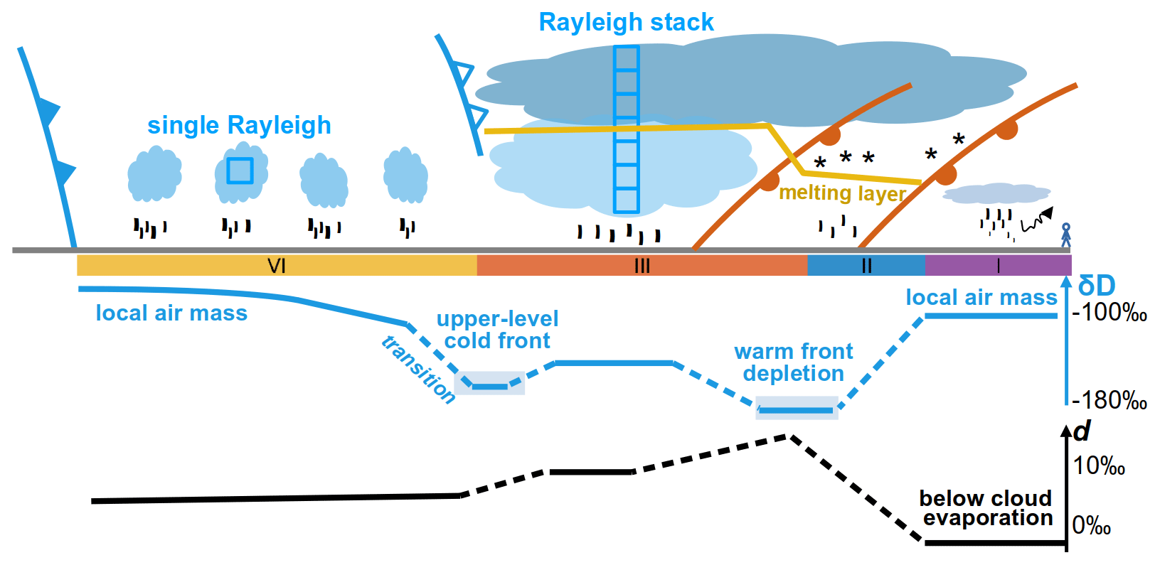
Figure 9 Weather diagram for the land-falling AR at Bergen on 7 December 2016. δD and d-excess lines represent the evolution of isotope composition of equilibrium vapour from surface precipitation. Precipitation periods (I, II, III, and IV) are indicated with colour bars at the bottom. Note that the timeline is from right to left.

Combining isotope and meteorological observations, we have identified four different precipitation stages during the event. At each stage, weather system processes imprint on the isotope variations (Fig. 9). Specifically, at the beginning of the event (Stage I), below-cloud evaporation is substantial, contributing to the low and even negative d-excess and relatively less depleted δD in surface precipitation. At Stage II, the gradual weakening of below-cloud evaporation as ambient air becomes more saturated and the involvement of hydrometeors from above the melting layer result in a gradual drop of δD and an increase in d-excess. At Stage III, deep clouds allow hydrometeors formed at high levels to gain moisture from low levels, leading to intermediately depleted values in δD. Stage IV is characterized by numerous convective showers that are formed at relatively low elevation, leading to the least depleted δD values during the event. The gradual drop of the d-excess in both surface precipitation and vapour during Stage III and IV can at least partly be explained by a change in moisture source conditions.

Regarding the controversial discussion of the isotope signal during previous AR events in the literature (Coplen et al., 2008; Yoshimura et al., 2010; Coplen et al., 2015), we emphasize from our results that the isotope signal in precipitation is intimately coupled to the cloud microphysics and dynamics. Idealized Rayleigh models may be adequate to represent the isotope composition of water vapour near cloud top during convective precipitation events. However, additional factors and more complex models should be considered to interpret the isotope signal in surface precipitation, in particular for deep, stratiform clouds. A stack of Rayleigh models could be a more adequate conceptual view for these cloud types (Fig. 9).

Our case study provides a unique isotope dataset of an AR event in southwestern Norway. More cases should be investigated in the future to test the more general validity of the results obtained in this case study. However, from one case, it is already apparent that the combined information from paired water vapour and precipitation sampling can be highly valuable for future data–model comparison studies with isotope-enabled weather prediction models.

Appendix A: Comparison of rain rate measurement

The rain rate at the sampling site (45 m a.s.l.) is measured by two instruments, i.e. a total precipitation sensor (TPS-3100) and Parsivel² disdrometer. Figure A1 shows a comparison of hourly rain rate during the precipitation period between the measurements of these two instruments and that of the rain gauge measurement from the closest meteorological station (70 m away, 12 m a.s.l.). The comparison shows that the TPS-3100 measures a slightly higher rain rate while the Parsivel² recorded a substantially lower rain rate, particularly in the situation of heavy precipitation. Since the TPS-3100 measurements agree well with the rain gauge measurements, we choose to use the rain rate from TPS-3100 for the analysis in this study. We did not choose to calibrate the TPS-3100 measurements against the rain gauge measurements because the small discrepancy can be due to the different locations and elevations of the two instruments.

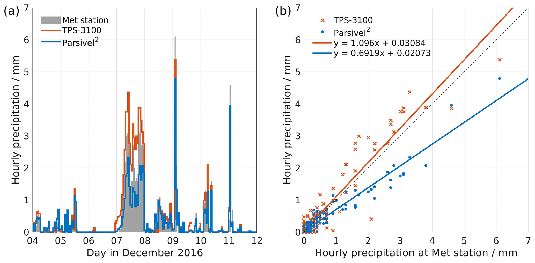
Figure A1 (a) Hourly rain rate during 4–11 December 2016 measured by rain gauge at WMO station (shading), TPS-3100 (red), and Parsivel² (blue). (b) Scatter plots and corresponding fits for the measurements of TPS-3100 (red cross) and Parsivel² (blue dot) against those from the rain gauge at WMO station.

Appendix B: Sensitivity studies with the Below-Cloud Interaction Model (BCIM)

Idealized simulations with the Below-Cloud Interaction Model (BCIM) model (Graf et al., 2019) help to reveal the sensitivity to factors influencing the below-cloud processes. The background thermodynamic profiles used by the BCIM model were here obtained from the moist adiabatic ascent of an air parcel that is lifted from the surface with initial values of T₀=5 ^∘C and RH₀=90 %. The background isotope profiles are obtained correspondingly from Rayleigh fractionation with a surface composition of $\mathit{\delta }\mathrm{D}=-\mathrm{160}$ ‰ and d-excess =10 ‰. A formation height of 1500 m was used in this reference simulation. All sensitivity simulations are obtained in the same way with an adiabatic ascent of an air parcel, while stepping through a range of drop sizes and modifying one of the initial values as detailed below.

• The sensitivity to RH was evaluated by modifying the surface RH in steps of 2 % between 64 % and 100 % while keeping all other parameters unchanged. The surface value for RH was interpolated linearly up to 100 % RH at the cloud base.

• The sensitivity to formation height was evaluated by modifying the formation height of the droplets in steps of 250 m from 500 to 3000 m while keeping all other parameters unchanged.

• The sensitivity to the temperature profile was evaluated by modifying the surface temperature in steps of 1 ^∘C while keeping all other parameters unchanged.

While BCIM provides helpful insights, its limitation should be noted. The model only considers a single falling hydrometeor and assumes that the background isotope profile of the atmosphere is not affected by evaporating hydrometeor or other processes during the simulation. However, in our AR case presented here, it can be clearly seen that the precipitation has a profound influence on the isotopic evolution of surface vapour.

The BCIM is available from the website https://git.app.uib.no/Harald.Sodemann/bcim (last access: 1 August 2021). More details of BCIM can be found in Graf et al. (2019).

Appendix C: Long-term observations and Lagrangian diagnostics

To examine our AR event in the context of the longer-term weather evolution, here we present selected observations at the sampling site as well as the Lagrangian moisture source diagnostics for the Bergen region between 4 and 11 December 2016 (Fig. C1).

A dry period of 1.5 d precedes the AR event. Following the AR event, discontinuous, moderate precipitation events occur (Fig. C1a). Comparison of the precipitation time series shows a qualitative agreement between the observation and Lagrangian diagnostic, with a substantial underestimation of precipitation intensity by Lagrangian diagnostic. The discrepancy in the precipitation intensity likely arises from the neglect of microphysical processes in the trajectory-based Lagrangian diagnostic and from the limitation of comparing a regional estimate with a single-point ground observation. The Lagrangian diagnostic shows that the dominating moisture source for the dry period prior to the AR event came from the north of Bergen (north of 65 ^∘N; Fig. C1b, black solid line). During the AR event, the moisture source shifted markedly to the south, reaching 35 ^∘N. After the AR event, the moisture source gradually shifts back to the north, reaching 55 ^∘N on 9 December, followed by another south-to-north variation. Closely following the source latitude, the moisture source distance reveals the air mass evolution from a local air mass prior to the AR event to a substantial remote air mass during the AR event and a moderate-distance air mass after the AR event (Fig. C1b, blue dashed line). The estimated RH_SST at the moisture source indicates relatively intense evaporation conditions at the moisture source before the AR event (RH_SST reaching 62 %), more moderate evaporation conditions during the AR event (RH_SST≈80 %), and varying evaporation conditions afterwards (RH_SST varying between 72 % and 85 %; Fig. C1c, black solid line). The local RH at the sampling site stays high (above 90 %) during the entire period, except at the beginning of the AR event and between 00:00 and 12:00 UTC on 9 December (Fig. C1c, blue dashed line).

Finally, we examine the d-excess of near-surface vapour, of equilibrium vapour from precipitation, and the d-excess estimation based on Lagrangian diagnostics (Fig. C1d). The d-excess of surface vapour exhibits a peak (above 8 ‰, with a maximum of about 16 ‰) during the first half day of the AR event. Thereafter, the d-excess of surface vapour remains at low levels mostly between 0 % and 8 ‰. The low d-excess can be due to the calm evaporation conditions at the moisture source or a contribution from land regions. The d-excess of equilibrium vapour from precipitation overall follows the variation in d-excess of surface vapour. The lower d-excess values for the quasi-daily precipitation samples collected after the AR event can be due to below-cloud evaporation and cloud microphysical processes.

Figure C1 The 7 d time series of observations at the sampling site and Lagrangian diagnostic (WaterSip) output for the Bergen region between 00:00 UTC 4 December and 00:00 UTC 11 December 2016. (a) The 6-hourly averaged rain rate observed from the total precipitation sensor (grey shading) and estimated rain rate from WaterSip (blue line). (b) Moisture source latitude (solid black line) and source distance (dashed blue line) estimated by WaterSip. (c) Moisture source RH_SST estimated by WaterSip (solid black line) and 6 h averaged RH at the sampling site (dashed blue line). (d) d-excess of the 10 min averaged vapour (grey dots), of the equilibrium vapour from precipitation (black segments) at 45 m above ground, and WaterSip estimate (light blue). The width of the black segment indicates the period over which the precipitation sample was collected. The uncertainties are 0.83 ‰ and 0.20 ‰ for d-excess of vapour and the equilibrium vapour from precipitation, respectively. The error bars in (a–d)  indicate 1 standard deviation. The missing data of the WaterSip at 12:00 UTC 6 December are due to bad data quality. The observation of d-excess is only available from 7 December.