the Creative Commons Attribution 4.0 License.
the Creative Commons Attribution 4.0 License.
 | 07 Sep 2022
Meridional-energy-transport extremes and the general circulation of Northern Hemisphere mid-latitudes: dominant weather regimes and preferred zonal wavenumbers
Federico Fabiano
Vera Melinda Galfi
Rune Grand Graversen
Valerio Lucarini
Gabriele Messori
The extratropical meridional energy transport in the atmosphere is fundamentally intermittent in nature, having extremes large enough to affect the net seasonal transport. Here, we investigate how these extreme transports are associated with the dynamics of the atmosphere at multiple spatial scales, from planetary to synoptic. We use the ERA5 reanalysis data to perform a wavenumber decomposition of meridional energy transport in the Northern Hemisphere mid-latitudes during winter and summer. We then relate extreme transport events to atmospheric circulation anomalies and dominant weather regimes, identified by clustering 500 hPa geopotential height fields. In general, planetary-scale waves determine the strength and meridional position of the synoptic-scale baroclinic activity with their phase and amplitude, but important differences emerge between seasons. During winter, large wavenumbers (k = 2–3) are key drivers of the meridional-energy-transport extremes, and planetary- and synoptic-scale transport extremes virtually never co-occur. In summer, extremes are associated with higher wavenumbers (k = 4–6), identified as synoptic-scale motions. We link these waves and the transport extremes to recent results on exceptionally strong and persistent co-occurring summertime heat waves across the Northern Hemisphere mid-latitudes. We show that the weather regime structures associated with these heat wave events are typical for extremely large poleward-energy-transport events.
- Article
(20860 KB) - Full-text XML
- BibTeX
- EndNote


The latitudinal gradient in incoming net solar radiation is the main trigger of atmospheric and oceanic dynamics (Peixoto and Oort, 1992). Indeed, the resulting energy imbalance induces an atmospheric circulation that causes divergence of heat at low latitudes and convergence at high latitudes. In the low latitudes, a key role is played by the zonally averaged circulation, dominated by the Hadley circulation, and the energy transport embedded in the mass streamfunction (Holton and Hakim, 2012). In the mid-latitudes, eddies are the most significant contributors to the overall transport.
Meridional energy transports through eddies are increasingly recognized as communicating the climate change signal towards the high latitudes, especially when taking into account the contribution by moisture (Hwang et al., 2011; Skific and Francis, 2013; Baggett and Lee, 2015; Rydsaa et al., 2021). Conventionally, the eddy contribution is partitioned into a transient and a stationary component, with the former identified as the instantaneous deviation from long-term climatology and the latter as the climatological departure from the zonal mean transport (e.g., Starr and White, 1954; Lorenz, 1967). Energy transports associated with transient eddies have been found to exhibit a large variability, with a number of sporadic extreme events exceeding the mean values by a few orders of magnitude (Swanson and Pierrehumbert, 1997; Messori and Czaja, 2013, 2015). This emphasizes the non-linear nature of baroclinic activity and its interactions at different wave scales and with the zonal-mean circulation (see Kaspi and Schneider, 2013; Messori and Czaja, 2014; Novak et al., 2015).
As an alternative to the usual transient–stationary eddy partitioning, a Fourier decomposition of eddy modes, isolating the contribution of different zonal wavenumbers to the overall transport has been proposed (Graversen and Burtu, 2016). Such zonal wavenumber decomposition relies on zonally integrated fluxes, meaning that spatially localized information is lost, and the contribution of different wavenumbers is provided in terms of the transport they effect across a given latitudinal circle. Despite this, it is still possible to link the results of the zonal wavenumber decomposition to the mid-latitude atmospheric circulation. For example, Graversen and Burtu (2016) found that latent energy convergence through planetary-scale waves is the most important contribution to the Arctic amplification, in agreement with Baggett and Lee (2015) and Boisvert and Stroeve (2015). Heiskanen et al. (2020) have also shown that planetary-scale waves have significantly increased their contribution in the last decades (cf. Rydsaa et al., 2021). These findings are placed in the context of ongoing debate on whether the decreasing meridional temperature gradient determined by Arctic amplification is setting more favorable conditions for the propagation and growth of planetary-scale waves (see Barnes and Polvani, 2013; Fabiano et al., 2021; White et al., 2022; Moon et al., 2022).
By separating synoptic and planetary scales as having wavenumbers k>5 or k = 1–5, respectively, it has been recently suggested that synoptic-scale eddies always allow for baroclinic conversion and thus systematically contribute to a poleward transport, while planetary-scale eddies can occasionally oppose the total transport resulting from the sum of all contributions (Lembo et al., 2019). A pronounced seasonal variability was also noticed, with planetary scales undergoing a much larger decrease from winter to summer than synoptic scales. Separating synoptic- and planetary-scale waves by wavenumber is inevitably arbitrary (Heiskanen et al., 2020; Stoll and Graversen, 2022); nonetheless, the results from Lembo et al. (2019) point towards the importance of modes of low-frequency, large-scale variability in modulating the energy transport by eddies (Messori and Czaja, 2015; Messori et al., 2017) and the emergence of preferred weather regimes in the occurrence of intermittent meridional-energy-transport extreme events (cf. Nie et al., 2008; Ruggieri et al., 2020). In a quasi-geostrophic context, the conversion of available potential energy into kinetic energy (Lorenz, 1955) supports the interpretation of the energy transfers in terms of modes of atmospheric variability. This then enables meridional-energy-transport variability to be linked to regional climate variability and extremes, as is particularly evident for climate extremes associated with specific circulation features, such as summertime blocks leading to heat waves (e.g., the 2010 summer event over Russia; Dole et al., 2011; Galfi and Lucarini, 2021).
Here, we focus on meridional energy transports in the mid-latitudes, where the baroclinic activity is strongest. We decompose the transport using the above-described zonal wavenumber decomposition approach of Graversen and Burtu (2016). Given the intermittent and sporadic nature of eddy-driven meridional energy transports described in Woods et al. (2013), Messori and Czaja (2013), and Messori and Czaja (2015), we focus on meridional-energy-transport extremes and analyze the associated circulation anomalies and weather regimes. Despite the known role of synoptic weather systems (e.g., Liu and Barnes, 2015) and storm tracks (e.g., Dufour et al., 2016) for the transfer of excess heat into the Arctic, our understanding of how these and other features of the mid-latitude atmospheric circulation may favor extreme transports is far from complete. We select the extremes with a rigorous methodology based on extreme-value theory (EVT) (Gnedenko, 1943). The extreme events are then associated with preferred patterns of the general circulation through k-means clustering of 500 hPa geopotential anomalies, identifying a set of weather regimes. The frequency of occurrence of such regimes is used to interpret the atmospheric circulation features associated with the occurrence of extremes in zonally integrated meridional energy transport. A composite mean analysis is also provided, highlighting some persistent patterns in specific regions of the NH (Northern Hemisphere) mid-latitudes.
The paper is organized as follows: in Sect. 2 we describe the data and the methodology for extreme-event selection and for the clustering of weather regimes. In Sect. 3a distributions of meridional energy transports, their wavenumber decomposition and their extremes as a function of latitude are described, while in Sect. 3b clustering of geopotential heights is related to composites of extreme events and dominant wavenumbers. In Sect. 4 an interpretation of these results is given, in light of composite mean anomaly patterns of geopotential height fields associated with extreme transports, while Sect. 5 summarizes the findings and outlines limitations and future perspectives.
2.1 Data
Data for meridional energy transport and atmospheric circulation analyses are obtained from the ERA5 Reanalysis (Hersbach et al., 2020), retrieved from the Copernicus Data Storage (CDS; Hersbach et al., 2018). The data used covers December–January–February (DJF) and June–July–August(JJA) from 1979 to 2012, with a 6-hour temporal resolution, a horizontal spatial resolution of 1∘ × 1∘ and 137 vertical levels. We deem the 6-hour temporal resolution sufficient to encompass the synoptic and larger modes of variability, as evidenced in recent analyses (Lembo et al., 2019). The choice of seasons is aimed at avoiding conflating regimes that are representative of the warm and cold seasons, as may happen in spring and autumn. The analysis is focused on the mid-latitudinal Northern Hemisphere band, i.e., latitudes in the 30–60∘ N range. For the computation of moist static energy, specific humidity (q), air temperature (T) and geopotential height (z) are considered. For the retrieval of the weather regimes and the k-means clustering, daily geopotential height at 500 hPa (z500) is used.
2.2 Methods
2.2.1 Meridional energy transports and wavenumber decomposition
The instantaneous meridional energy transport (or, more correctly, the enthalpy transport; cf. Ambaum, 2010; Lucarini and Ragone, 2011) is obtained as the scalar product of the meridional velocity v and the total energy E, including the kinetic energy and the moist static energy H, defined as
where q is the specific humidity; T is the air temperature; z is the geopotential height; and Lv, cp and g are the latent heat of vaporization, the specific heat at constant pressure and the gravity acceleration, respectively. The transport of E across a given latitude is computed with the vertical and zonal integration:
where ps is the surface pressure, and V is the horizontal velocity vector. The sign convention is that transport is positive when northward-directed and negative when southward-directed. The wavenumber decomposition is extensively discussed in Graversen and Burtu (2016) and in Lembo et al. (2019). Here, we recall that the meridional energy transport as a function of zonal wavenumber k can be written as
where a and b are the Fourier coefficients defined as
where Ψ is either v or E; D=2πRcos (ϕ) with R being the Earth's radius; k being the zonal wavenumber; t, ϕ and λ the time, latitude and longitude, respectively; and d = 360∘. The simple form in Eq. (4) is made possible by the fact that the k-members of the Fourier decomposition are harmonics in a cylindrical symmetry. Parseval's theorem then ensures that the cross-terms in the multiplication of the two Fourier series cancel each other when integrated over a latitude circle (Tolstov, 2012).
The highest zonal wavenumber N is set to 20, given that the spatial and temporal resolution of the ERA5 outputs poses a constraint to the modes of variability that can be resolved and since it has been shown that the transport associated with wave number 0 to 20 constitutes almost entirely the total transport (Graversen and Burtu, 2016). For the sake of conciseness, we group wavenumbers into: k = 0, reflecting zonal mean transports; k = 1–5 for planetary-scale transports; k = 6–10 for synoptic-scale transports; and k = 11–20 as mesoscale and lower-spatial-scale transports. The choice of thresholds for separating main eddy modes is somewhat arbitrary. Here, we follow the choice made in Graversen and Burtu (2016) and subsequently in Lembo et al. (2019) to ensure easy inter-comparability of results. Although there are also arguments supporting other threshold choices (cf. Heiskanen et al., 2020; Stoll and Graversen, 2022; see also Appendix C), earlier studies of different impact of planetary- versus synoptic-scale waves have revealed that decomposition of the transport into these wave types is not dependent on the choice of the threshold for wave grouping (Heiskanen et al., 2020; Stoll and Graversen, 2022).
The meridional circulation includes a zonal mean mass transport in opposite direction at different altitudes. However, at small temporal scales a vertical mean mass transport across latitudes may be encountered, which may transport a large amount of energy. This latter component of the enthalpy transport has to be subtracted from wave zero transport in order to obtain the energy transport by the mean meridional circulation (Liang et al., 2017), which is done following Lembo et al. (2019). The instantaneous zonal-mean and vertical-mean meridional-circulation-energy-transport component is thus written as
with { } denoting the vertical mean, [ ] the zonal mean and † the departure from the vertical mean. Note that the wave zero energy transport component is given by the first term on the right-hand side of Eq. (7).
2.2.2 Selection of the extreme events
We adopt in this work a rigorous methodology for the detection of meridional-energy-transport extremes based on the “peak over threshold” approach of extreme-value theory (EVT) (Balkema and de Haan, 1974; Pickands, 1975). The main advantage of this methodology is that the properties of the data themselves determine the threshold used to define extreme events instead of arbitrary threshold choices. Furthermore, the probability distribution of extreme values is given by EVT; thus no subjective decisions are needed considering the shape of this distribution. An overview of this approach is hereby drawn, based on Coles et al. (2001), and of the convergence algorithm also presented in Gálfi et al. (2017). Full theoretical and technical details can be found therein.
We first consider a series of independent identically distributed random variables with common probability distribution F(X), X denoting an arbitrary term in the series Xi. Under appropriate conditions (discussed generally below; for a comprehensive and rigorous description see Leadbetter, 1974, Leadbetter et al., 1989 and Coles et al., 2001), the threshold exceedances y of a large enough threshold u, with X>u, are asymptotically distributed according to the generalized Pareto distribution (GPD) family as
with for ξ≠0, y>0, and σ>0. The shape parameter ξ determines the shape of the distribution and the tail behavior. If ξ=0, the tail of the distribution decays exponentially, and if ξ>0, the tail decays polynomially, while, if ξ<0, the distribution is bounded.
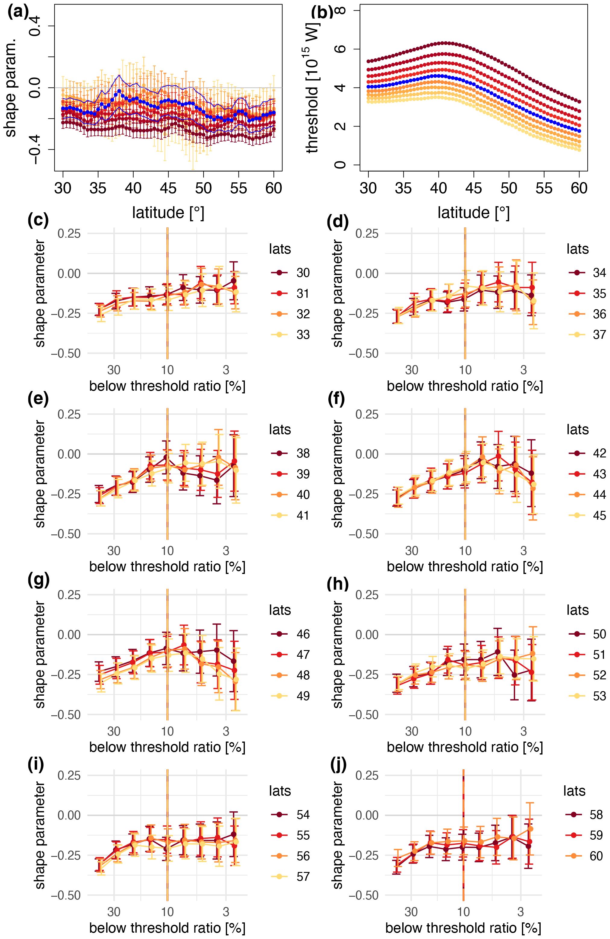
Figure 1Meridional section for equatorward DJF meridional-energy-transport extremes of (a) shape parameter ξ (non-dimensional) and (b) threshold value [1015 W]. The colors in (a) denote parameter estimates corresponding to the threshold values shown in (b). The blue lines denote the final shape and scale parameter estimates based on the blue threshold values. (c–j) Shape parameter as a function of threshold (in terms of fraction of data points below the threshold) at different latitudes. The uncertainty range is defined based on 95 % maximum likelihood confidence intervals. The vertical orange line denotes the selected fraction of data for the specific tail, which is chosen to be the same at all latitudes.
In order to apply EVT to meridional-energy-transport data, one has to make sure that the conditions of independence and homogeneity are fulfilled, and thus the data can be modeled based on a stationary stochastic process (Leadbetter, 1974). While both conditions are, strictly speaking, unrealistic in the case of geophysical data, the problem can be approached from a practical perspective. First, we detect linear long-term trends for the 1979–2012 period, and we test their significance according to a Mann–Kendall test at the 95 % significance level (Mann, 1945; Forthofer and Lehnen, 1981), then we remove trends only at those latitudes where they are found to be significant, i.e., for DJF, north of 37.5∘ N and for JJA in the 40–47.5∘ N and 54.5–58.5∘ N latitudinal bands. By analyzing summer and winter separately, we eliminate another source of dependence and heterogeneity due to the seasonal cycle. Furthermore, we verify for every latitude the decay of the auto-correlation function. Despite the fact that several consecutive values in our time series are correlated, the chaotic nature of atmospheric motions allows two values far away in time from each other to be nearly independent, meaning that the auto-correlation function decays to 0 at a finite time lag. Looking at the auto-correlation functions, we find that JJA (DJF) daily data require the removal of the climatological JJA (DJF) season at every latitude (south of 45∘ N). Given that the non-homogeneous detrending and deseasonalization may in principle introduce discontinuities, we compared results obtained with the described method to those obtained when the two corrections were applied at all latitudes (not shown). The small discontinuity found at latitude 45∘ N in the meridional section of threshold values (Fig. 1b) was indeed removed when the corrections were applied at all latitudes, but the difference is minimal. Finally, the GPD parameters were computed. Even in the absence of long-range correlations, however, one may encounter clusters of data exceeding the threshold consecutively in time. Those are clearly correlated and would lead to biased GPD parameters1 as a result of a slower convergence to the limiting distribution (Coles et al., 2001). To avoid this, we decluster, where necessary, the time series before estimating the parameters by using the “intervals” declustering method (Ferro and Segers, 2003) based on the “extremal index” defined in Gálfi et al. (2017).
We then test the applicability of the theory by looking at the convergence of the selected extremes to the limiting GPD distribution. This is done by plotting the estimated shape parameter ξ(u) as a function of an increasing threshold u (cf. Fig. 1). By visual inspection, for the right (left) tail of the probability density function (PDF), the lowest (highest) threshold u∗ at which the shape parameter becomes stable, i.e., does not change with further threshold increase (decrease), provides the optimal parameter estimate. This estimate has a lower uncertainty than the ones for (), and, at the same time, the distribution of the selected extremes is equivalent to the limiting GPD, in the limits of estimation uncertainty given by the confidence intervals. In order to achieve a latitude-independent definition of extremes, we express the threshold in terms of fraction of data points above (below) the threshold and the total number of data points. For each tail of the distribution, the same threshold is provided at all latitudes, given as the highest fraction of data points for which the convergence is achieved at all latitudes.
This threshold selection procedure applies in the case of extremes located in the right tail of the transport's probability density function (PDF), hereafter referred to as “poleward” extreme energy transports. Similarly, we refer to extremes located in the left tail of the PDF as “equatorward” extreme energy transports. These extremes are weaker than the median transports and sometimes slightly negative. The procedure for equatorward extremes is the same as described above for poleward extremes. Hence, we search for a stable shape parameter as a function of a decreasing threshold, equivalent to a decreasing fraction of data points below the threshold.
For illustrative purposes, Fig. 1 shows the behavior of the shape parameter ξ as a function of the threshold u at different latitudes. We notice that the shape parameter is negative almost everywhere, evidencing that the extreme-value distribution is bounded. In other words, Fig. 1 provides a graphical explanation of the convergence methodology, justifying the following choice of the thresholds:
-
DJF, equatorward – 10 % of data below the threshold (10 % percentile);
-
DJF, poleward – 14 % above the threshold (86 % percentile);
-
JJA, equatorward – 14 % below the threshold (14 % percentile);
-
JJA, poleward – 7 % above the threshold (93 % percentile).
We notice that, while ξ is systematically negative for this choice of the thresholds, σ is positive and slightly increasing with latitude, denoting an increasingly large spread of extremal values (Fig. 1a and b).
2.2.3 Weather regimes
The weather regimes (WRs) are computed from the daily geopotential height at 500 hPa (z500), using the WRtool Python package (Fabiano et al., 2021). We summarize the methodology here; for more details and discussion the reader is referred to the “Methods” section in Fabiano et al. (2020). We focus on latitudes between 30 and 90∘ N and three different longitudinal sectors: the Euro–Atlantic (EAT; from 80∘ W to 40∘ E), the Pacific–North American (PAC; from 140∘ E to 80∘ W) and the whole Northern Hemisphere mid-latitudes (NH).
The original data were first interpolated to 2.5∘ × 2.5∘ horizontal resolution; since the WR diagnostic aims at capturing large-scale configurations, this step does not alter the results of the analysis. Before computation, the daily mean seasonal cycle – smoothed with a 20 d running mean – is removed from the data to obtain daily anomalies.
To retain only the large-scale component and reduce dimensionality, an empirical orthogonal function (EOF) decomposition is performed, separately for each considered longitudinal sector. The minimum number of EOFs that explain at least 90 % of the total variance is retained: this corresponds to 16, 19 and 41 EOFs during DJF for the EAT, PAC and NH, respectively, and 22, 25 and 57, respectively, during JJA. An EOF-based dimensionality reduction is a common first step in weather regime detection algorithms (Cassou, 2008; Dawson et al., 2012; Cattiaux et al., 2013; Straus et al., 2017; Dorrington et al., 2022). Sensitivity tests on the number of EOFs retained (not shown) confirm that the regime patterns are robust to this choice (e.g., Fabiano et al., 2020), with the full field recovered in the limit of all EOFs. The fact that higher-rank EOFs do not provide a significant advantage in terms of accuracy of the clustering implies that they denote mainly noise. The WRs are then computed by applying a k-means clustering algorithm to the selected principal components (PCs). Appendix B highlights that differences in the distribution of the first four PCs between the full population (all days) and the population of extreme events are consistent with the differences observed in the weather regime frequencies, offering a complementary view. Although EOFs in the two populations can still be significantly different, this suggests that weather regimes are a fundamental representation of the dynamics and are thus suitable to investigate the differing statistics of the extremes relative to the overall population.
For all sectors and seasons, we set the number of regimes to 4. This choice is widely documented in the literature for the EAT and PAC winter circulation (Michelangeli et al., 1995; Cassou, 2008; Weisheimer et al., 2014; Hannachi et al., 2017; Straus et al., 2017), although different numbers of clusters have been used in other studies (e.g., Pasquier et al., 2019; Strommen et al., 2019; Hochman et al., 2021). Each day is assigned to one of the regimes, and a set of four regime centroids is obtained. The regime pattern is defined as the composite of all anomalies assigned to a certain regime.
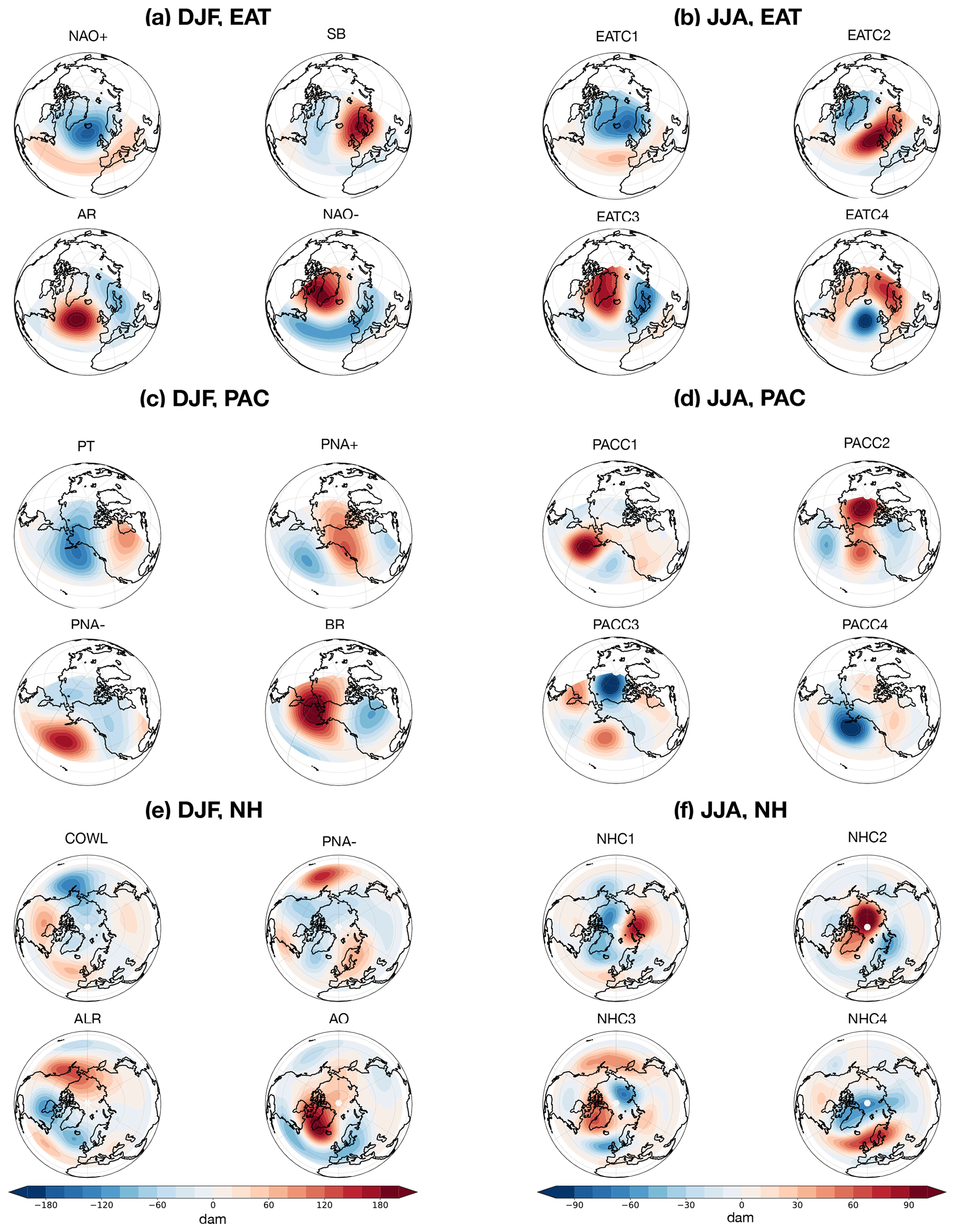
Figure 2Clusters of zg500 geopotential height anomalies (in dam) by frequency in (a) DJF, computed over the EAT region; (c) DJF, computed over the PAC region; (e) DJF, computed over the NH region; (b) JJA, computed over the EAT region; (d) JJA, computed over the PAC region; and (f) JJA, computed over the NH region.
Figure 2 shows the pattern of the weather regimes computed for each region (EAT, PAC, NH) and season (DJF, JJA) during 1979–2012, following the procedure described above. DJF patterns (left column) resemble the conventional DJF weather regimes in the literature. These are, for EAT, the North Atlantic Oscillation (NAO) positive phase (hereafter NAO+), the Scandinavian blocking (SC), the Atlantic Ridge (AR) and the NAO negative phase (NAO−) (Cassou, 2008; Dawson et al., 2012); for PAC they are the Pacific trough (PT), the positive and negative phases of the Pacific–North American pattern (PNA+, PNA−), and the Bering Ridge (BR) (Jung et al., 2005; Weisheimer et al., 2014; Straus et al., 2017); and for NH they are the “cold ocean–warm land” pattern (COWL), the PNA−, the Aleutinian Ridge (ALR) and the Arctic Oscillation negative pattern (AO) (cf. Kimoto and Ghil, 1993; Corti et al., 1999).
We refer to JJA regimes (right column) as xCn, with “x” being EAT, PAC or NH and the index denoting the cluster. Thus, for the EAT domain, EATC1 features a zonally spread blocking extending from the eastern Atlantic to Scandinavia; EATC2 closely resembles the NAO+ pattern; EATC3 can be referred to as a Greenland blocking; and EATC4 features a dipole structure, with an eastern Atlantic low and a Scandinavian high (cf. Guemas et al., 2010; Yiou et al., 2011). Concerning PAC and NH, all regimes feature anomalies that are much weaker than DJF regimes, given that the circulation as a whole is weaker in the JJA season. PACC1 features a weak blocking southwest of Alaska, while PACC2 is somehow similar to the BR pattern, although much weaker. PACC3 and PACC4 appear to mirror each other. NHC1 exhibits a Siberian high, while NHC2 features a number of highs surrounding the North Pole; NHC3 features a Greenland blocking, and NHC4 closely resembles EATC1.
As shown in Fig. 2, the weather regimes are weaker in summer than in winter, consistent with the seasonal cycle of atmospheric variability (e.g., Faranda et al., 2017). Hence, despite in some cases being apparently similar, weather regimes in the two seasons hint at genuinely different aspects of the dynamics, as further discussed in Sect. 3.2.
For each cluster, the absolute frequency is computed within the population of all events, then the ratio of absolute frequency in the population of extreme events to the absolute frequency in the overall population is obtained, for each tail of the distribution and in each season. Specifically, the relative variations in absolute frequencies are retrieved as , where fx is the absolute frequency of occurrence of the cluster x for the overall population, and is the frequency of occurrence of extreme events in cluster x relative to the total extreme population. Hence a positive indicates that cluster x includes a higher fraction of extreme events compared to its fraction of all events; i.e., cluster x is more favorable for extreme events. In order to assess whether the variation in absolute frequencies is significant, a bootstrapping is performed, through 300 random resamplings of the original population with the same number of events as the number of extreme events in the respective tail. The hypothesis test is performed at the one-sided 95 % significance level.
In order to link the weather regime characterization of extremal transports to the wavenumber decomposition illustrated in Sect. 3.1, we focus on the zonal wavenumber effecting the largest share of the meridional-energy-transport anomaly. First, at each latitudinal band, for each assigned weather regime, in each season and for each tail of the distribution, we compute the contribution of each individual wavenumber to the meridional-energy-transport anomaly with respect to the average across the extreme events in the selected subset. Then, the dominant wavenumber for the specific event is assigned as the one whose contribution to the transport is largest. Finally, the average of the dominant wavenumbers across the subset of extreme events assigned to the specific regime and occurring at the selected latitudinal band is computed.
3.1 The PDFs of meridional energy transports and their wavenumber decomposition
We start our analysis by looking at the PDFs of the total and wavenumber-decomposed meridional energy transports and their extremes.
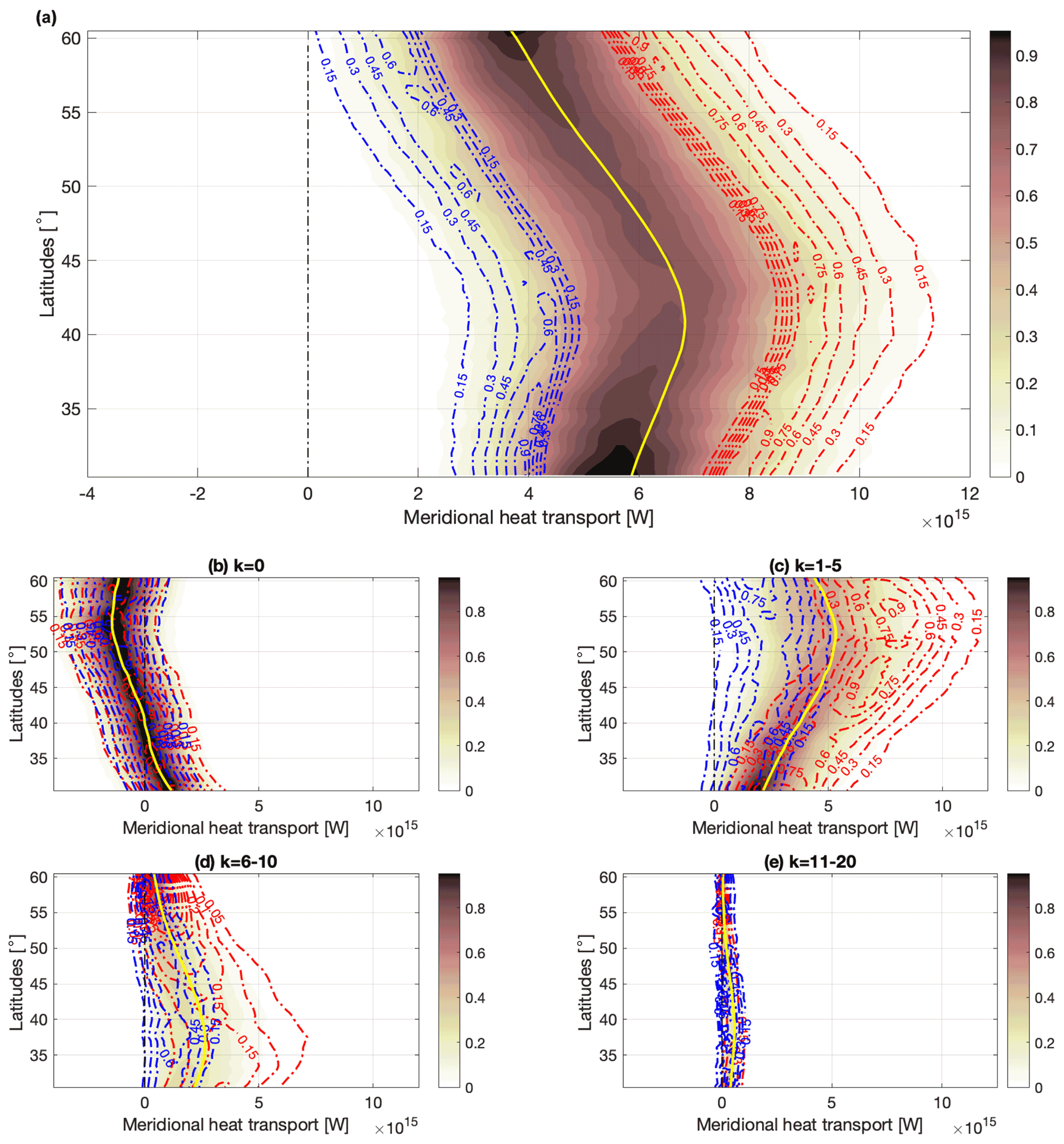
Figure 3PDFs of total (filled contours) and extreme poleward (red contours) and equatorward (blue contours) DJF meridional energy transports over the 1979–2012 period in ERA5. (a) Sum of all wavenumber contributions, (b) k = 0 (zonal mean), (c) k = 1–5 (planetary scales), (d) k = 6–10 (synoptic scales), (e) k = 11–20 (higher scales). PDFs are normalized dividing by the maximum value across all latitudes. In order to account for the different range of extremes at different latitudes, the Freedman–Diaconis rule (Freedman and Diaconis, 1981) is first applied to determine the correct number of bin elements for the discretized PDF, then the kernel smoothing estimate (Bowman and Azzalini, 1997) is computed. For graphical purposes, at each latitude the obtained PDFs for the extremes are interpolated on the same number of bins as the PDFs of the overall population.
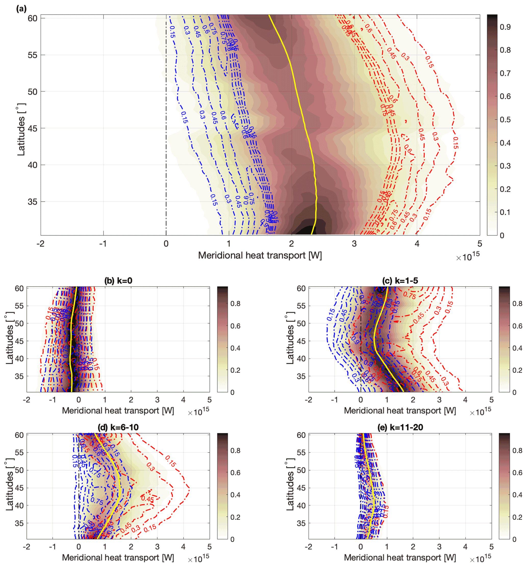

Figure 5Unbiased estimates of meridional-energy-transport skewness, as a function of latitude, for (a) PDF across all events, (b) equatorward extremes only and (c) poleward extremes only. Solid lines denote DJF, dashed lines JJA.
The PDFs (filled contour plots) of the total zonally averaged meridional energy transport are computed for each latitude in the 30–60∘ latitudinal band, as shown in the top panels of Figs. 3 and 4 (for DJF and JJA, respectively). A normalization is performed across latitudes in order to evidence the diversity of ranges at different latitudes. In DJF, the PDF peaks at about 42.5∘ N, with a value of 6.5 × 10¹⁵ W; the mean of the PDF then decreases towards the higher latitudes. In JJA, the PDF shows a weaker variability across latitudes, with a mean and median value oscillating between 2.0 and 2.5 × 10¹⁵ W and a moderate decrease towards the high latitudes. PDFs in DJF are overall positively skewed, as shown in Fig. 5. The highest skewness (about 0.4) is at the equatorward edge of the mid-latitudinal band, while the lowest skewness (0.2) is in proximity of the median peak of the total transport around 45∘ N. In JJA, the PDF is more skewed north of 40∘ N, with values ranging between 0.3 and 0.25, whereas it is more symmetric south of 35∘ N, with values of about 0.1. A positive skewness indicates that the PDFs are asymmetric, with a larger or longer tail of positive (“poleward”) than negative (“equatorward”) extremes. The skewness values are consistent with the eddy circulation in mid-latitudes favoring intermittent, locally strong poleward transports that also have a signature in the zonally integrated transport (cf. Messori and Czaja, 2015; Marcheggiani et al., 2022).
The extreme transports for both equatorward and poleward tails of the distributions are identified from the PDFs of total zonally averaged transports, following the methodology described in Sect. 2.2.2. Both sets of extreme transports are heavily skewed in both seasons, with poleward extremes being more skewed than equatorward extremes (Fig. 5). The asymmetry of the total transports is consistent with this slight difference. In the overall PDFs, meridional sections of DJF and JJA skewness are opposed, with larger values at the equatorward edge in DJF, in the center of the mid-latitudinal band in JJA. The larger skewness at the equatorward edge hints at the presence of relatively larger extreme transports, where the non-linear growth of the baroclinic waves is more pronounced (Novak et al., 2015), despite the median transport being weaker than at the center of the domain. This is also mirrored in the meridional section of DJF skewness for poleward extremes (Fig. 5c). Equatorward extremes attain smaller or even negative values at high latitudes, where the mean transport is weaker, which emphasizes the importance of such extreme events for setting the seasonal energy transport at high latitudes. The opposite occurs for the poleward extremes, with the largest extremes being stronger for those latitudes where the mean transport is stronger. This is in agreement with Lembo et al. (2019), who found that both poleward and equatorward extremes are related to the mean strength of the transport (cf. their Fig. 1d–g).
We next decompose the transport into its wavenumber components in Figs. 3c–f and 4c–f. Similarly, the extreme values sampled from the PDF of the total transports are decomposed in wavenumbers. In both seasons the most significant contribution to the overall transport comes from the planetary-scale and synoptic-scale contributions. The equatorward and poleward extremes largely overlap in the zonal mean component, and both attain negative values, while the zonal mean component does not provide a significant contribution to the extreme transport. Very different features emerge at the planetary and synoptic scales. During DJF and at both these scales, the magnitude of poleward extremes follows that of the median transport for the respective component and attains large values when the median component is at its maximum. Equatorward extremes, on the other hand, only partly follow the median curve and attain near-zero values at almost all latitudes, especially regarding the synoptic contribution. During JJA, a significant share of planetary-scale equatorward extremes feature net negative transport in the middle latitudes, where the contribution to the transport is almost vanishing on average. This is consistent with planetary waves being able to act passively, transporting energy counter-gradient, and thus with no conversion of available potential energy into kinetic energy, as discussed in Baggett and Lee (2015) and Lembo et al. (2019). Synoptic-scale waves, instead, almost everywhere share the positive sign and the meridional structure of the mean transport, although as in DJF, the most extreme events during JJA also attain near-zero values at almost all latitudes.
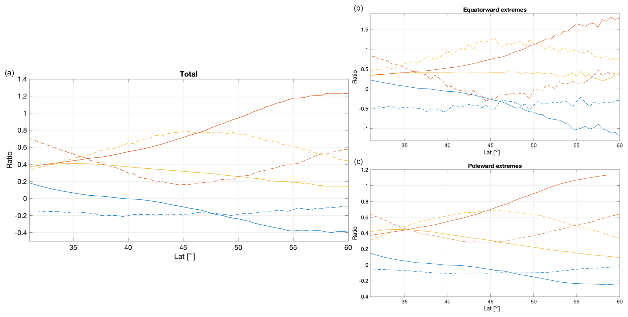
Figure 6Ratios of zonal (blue), planetary (red) and synoptic (yellow) wavenumber components for all events (a), equatorward extremes (b) and poleward extremes (c). Solid lines denote DJF, and dashed lines denote JJA.
To provide a clearer view of the relative importance of the different components, we show in Fig. 6 meridional sections of the ratios of zonal (in blue), planetary (in red) and synoptic (in yellow) scales to the total transports and their extremes for the two seasons. The latitudinal gradient is largest in DJF, with the planetary scales becoming relatively more important (up to 1.2 times the total transport) and the synoptic scales decreasing (starting from 0.4 at 30∘ N to 0.1 at 60∘ N) with increasing latitude. The zonal component, in turn, has the same sign as the total transport in the lower latitudes, then turns negative and opposes the eddy components, having a ratio of up to 0.4 of the total transport. In JJA, the relative ratios of the planetary and synoptic component are antisymmetric, and the zonal component is steadily negative, opposing the eddy transport. Extreme transports show similar features, with the ratio of planetary scales in JJA equatorward extremes becoming negative around 45∘ N and remaining small at higher latitudes, while the zonal component consistently opposed about half of the total poleward transport at all latitudes. The planetary and synoptic scales thus rarely contribute in a similar way to the overall transport, and this is especially true for the extremes. Indeed, planetary and synoptic extremes are rarely happening concomitantly, as already found in Lembo et al. (2019).
3.2 Weather regimes and zonal wavenumbers associated with extreme events
We now shift our attention to the detection of weather regimes in the population of extreme events, in order to investigate the relation between extreme transports and recurrent patterns of the large-scale circulation.
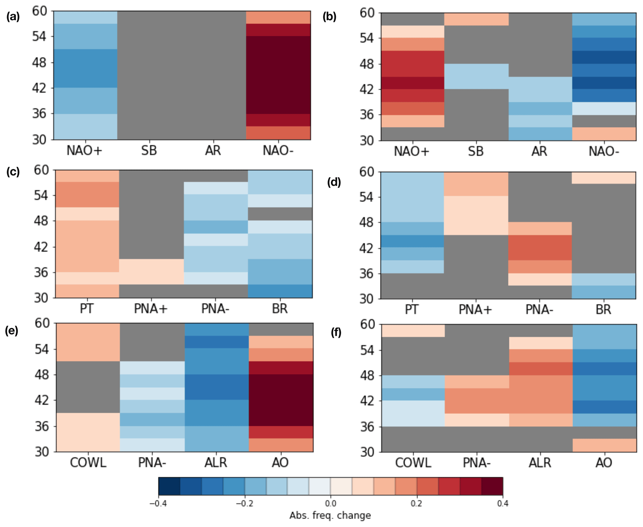
Figure 7Relative variations in absolute frequency of clusters in the population of DJF extremes as a function of the latitude at which extremes are found: (a) EAT region, poleward extremes; (b) EAT region, equatorward extremes; (c) PAC region, poleward extremes; (d) PAC region, equatorward extremes; (e) NH region, poleward extremes; (f) NH region, equatorward extremes. Gray boxes denote non-significant frequency variations, according to the bootstrapping methodology described in the “Methods” section.
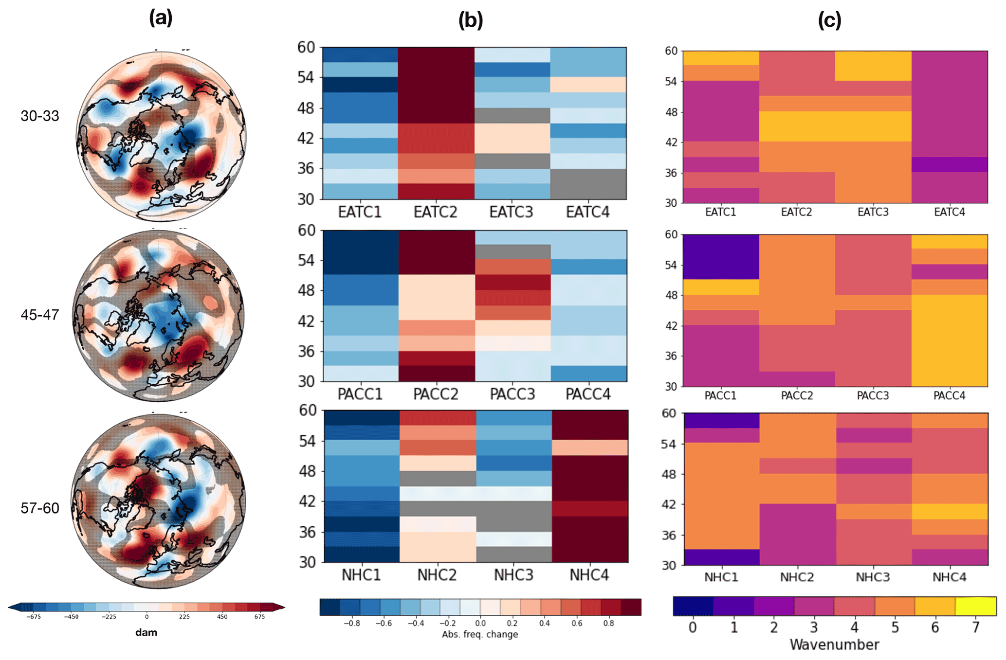
As discussed in Appendix B, conditioning on different extreme transport events yields different average values of the PCs of the leading EOFs, suggesting that the population of extreme events might exhibit a preferred development of specific weather regimes. Following from this hypothesis, we compute in the population of extreme events (as described in Sect. 2.2.3), grouping extremes by 2∘ wide latitudinal bins. Figures 7 and 8 display for each of the chosen regimes in the EAT, PAC and NH regions, for poleward (left) and equatorward (right) extreme events in DJF and JJA, respectively.
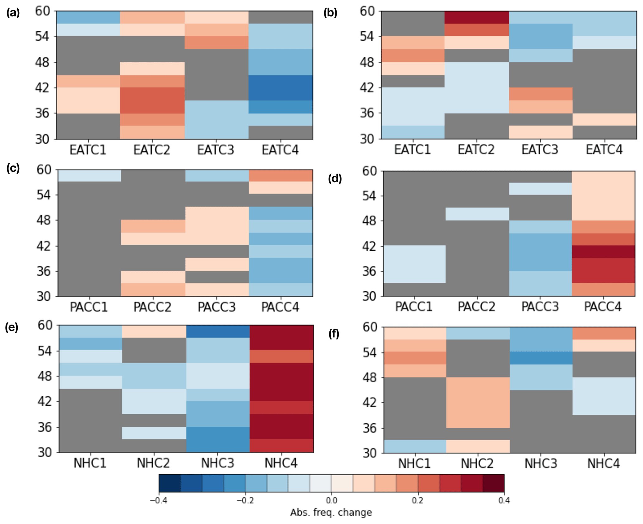
DJF poleward extremes are characterized by anomalously negative z500 anomalies in the lower mid-latitudes and high-latitudinal blockings over the northern Atlantic, as denoted by stronger frequency of NAO− (Fig. 7a) and AO (Fig. 7e) during extreme events. In the Pacific region, PT (Fig. 7c) regime frequency increase denotes large meridional exchanges with wide ridges and troughs. Consistently, a significant reduction in the NAO+, BR and ALR modes is found. In JJA, NHC4–EATC2 (Fig. 8a and e), characterized by a pattern similar to an eastern Atlantic–Scandinavian blocking, is increasingly likely. EATC4 (Fig. 8a) and PACC4 (Fig. 8c), denoted by negative anomalies in the eastern boundaries of the Atlantic and Pacific oceans, are rarer, as well as NHC3 (Fig. 8e), featuring a weak Pacific ridge and a Greenland blocking. In general, we observe that changes in absolute frequencies are coherent across neighboring latitudes, consistent with what is observed for the energy transport extremes, often occurring concomitantly at several latitudes (compare to Fig. 1d–g in Lembo et al., 2019).
DJF equatorward extremes largely mirror what is described for poleward extremes: NAO− (Fig. 7b), PT (Fig. 7d) and AO (Fig. 7f) modes become generally less frequent, whereas NAO+, PNA−, ALR and, to some extent, BR modes are more frequent. In other words, a more zonal North Atlantic regime and stronger Pacific blocking are associated with weaker meridional transports. This is in line with the opposite signs of PC fractional changes described in Appendix B. Looking at JJA, it clearly emerges that the PACC4 (Fig. 8d) pattern becomes more frequent, while PACC3 (Fig. 8d) and NHC3 (Fig. 8f) (especially for extremes at high latitudes) are rarer. Remarkably, EATC3 and EATC1 (Fig. 8b) become increasingly likely for extremes at low and mid-latitudes, respectively, and EATC2 becomes increasingly likely for extremes at higher latitudes. This suggests a weakening and a northward shift of the centers of baroclinic activity as the latitude at which the equatorward extremes are selected increases, although a direct comparison is not provided here.
We then focus our attention to the dominant wavenumber, as a function of the region and of the weather regime to which extreme events are attributed. We remark that the spectrum of the meridional energy transports is now different from the one considered in Figs. 3 and 4 as we focus on the wavenumber decomposition anomalies relative to their climatological contributions rather than on their absolute values. For this reason, we limit our range of wavenumbers to 0–7 as no higher wavenumber appears to be dominant in any of the considered cases.
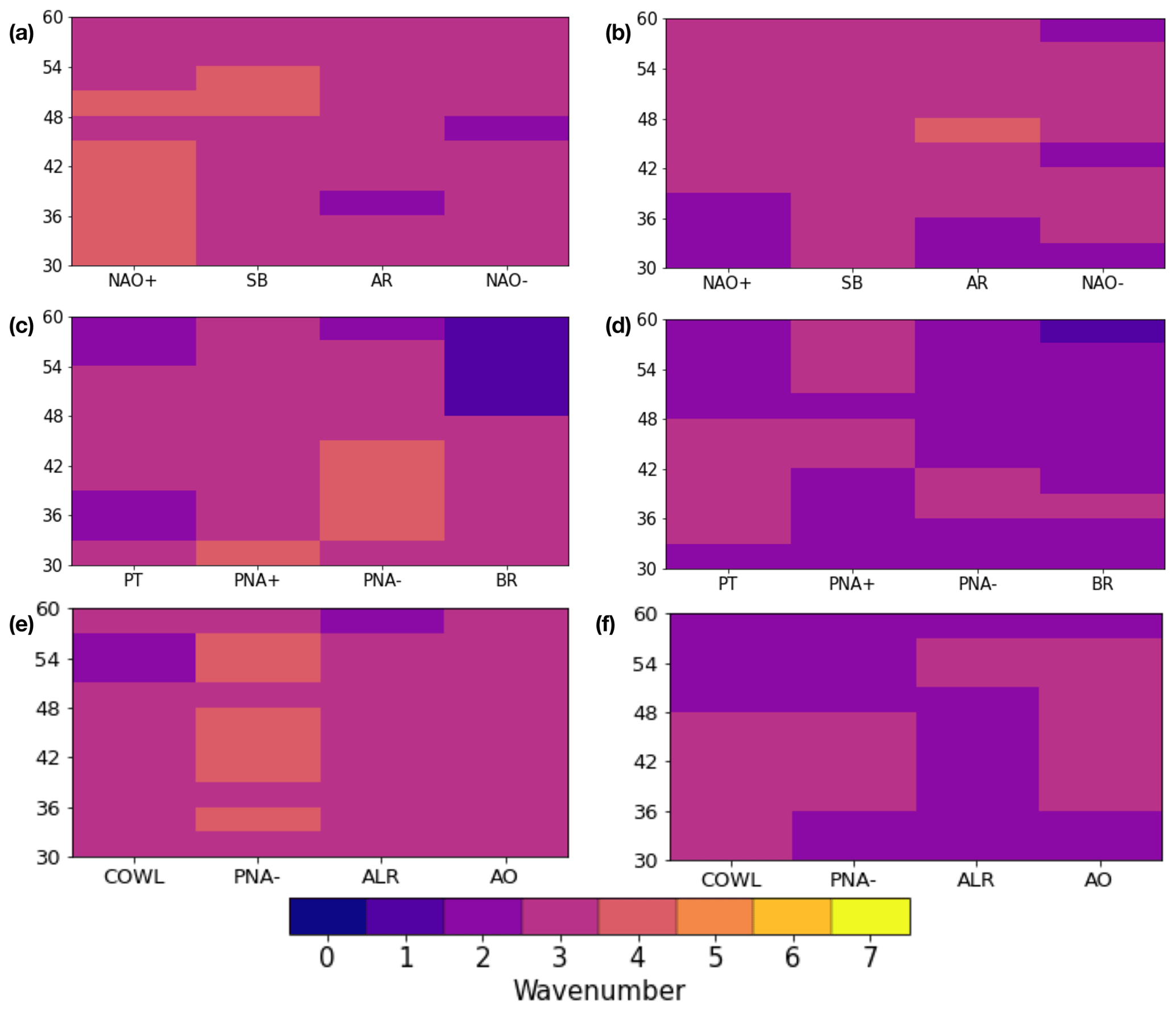
Figure 9Time-averaged zonal wavenumber associated with meridional-energy-transport extremes (see text) for DJF clusters obtained in different regions, as a function of the latitude at which the extreme is found. (a) EAT region, poleward extremes; (b) EAT region, equatorward extremes; (c) PAC region, poleward extremes; (d) PAC region, equatorward extremes; (e) NH region, poleward extremes; (f) NH region, equatorward extremes.

No matter in which region the clustering is focused, DJF extreme events are associated with dominant wavenumbers between 2 and 4 (Fig. 7). In JJA (Fig. 10), the situation is more diversified, with dominant wavenumbers in the range of and a clearer dependence on the circulation cluster. The dominance of higher zonal wavenumbers is consistent with the finding that PC fractional changes in JJA occur mainly for higher-order EOFs, as described in Appendix B. Poleward extremes generally peak at higher wavenumbers than equatorward extremes. Focusing on EATC2 and NHC4, we also find that scales bridging the chosen planetary–synoptic threshold (k=5 and k=6) are co-located with latitudes featuring the largest frequency change (cf. Fig. 8). Interestingly, to some extent the same happens for EATC4, PACC4 and NHC3, where the latitudes featuring the largest frequency reductions are also characterized by relatively higher wavenumbers (compared to extremes in other clusters and in the same cluster but different latitudes), again k=5 and k=6. Dominant wavenumbers for equatorward extremes are less sensitive to frequency variations: events associated with PACC4 and EATC1 frequency increases are associated with a dominant k=4 wavenumber. EATC2 features a k=3 dominant wavenumber in the high latitudes, whereas EATC3 is characterized by a k=2 wavenumber in the low latitudes.
The zonal wavenumber decomposition adopted here poses some challenges when trying to relate meridional-energy-transport extremes to specific atmospheric circulation features. Above, we have adopted weather regimes as a tool to identify such circulation features, and we argue that they span the diversity of patterns associated with these extremes. In order to further examine the population of extreme transport events and identify persistent patterns in some regions of the domain, it is useful to complement the description of weather regimes and dominant wavenumbers with the analysis of composite mean z500 anomalies. We stress that while the composite mean view is not informative of the intrinsic variability associated with those extreme events, it allows already-evidenced aspects of the circulation associated with extreme transport events to be better framed. Figures 11 and 12 display composite mean z500 anomalies for meridional-energy-transport extremes taken at three different latitudes in JJA and DJF, respectively. Table 1 shows that latitudinal variations in the number of events are within 10 % of the sample size, ensuring that the anomaly maps in the two seasons have comparable significance. Clearly, DJF and JJA differ in the fact that the higher zonal variability in the latter is related to a higher dominant zonal wavenumber. The emergence of patterns consistent with the dominant wavenumbers highlighted in Figs. 9 and 10 hints at the amplitude of such waves as determining the strength of the transport.

Figure 11Composite mean of z500 anomalies (in dam) for JJA (a) poleward and (b) equatorward meridional-energy-transport extremes at three chosen latitudinal bands. Non-significant values are shaded in gray. The significance is tested with a bootstrapping method at the 95 % significance level. The null hypothesis is that the composite mean value lies within the range of internal variability.
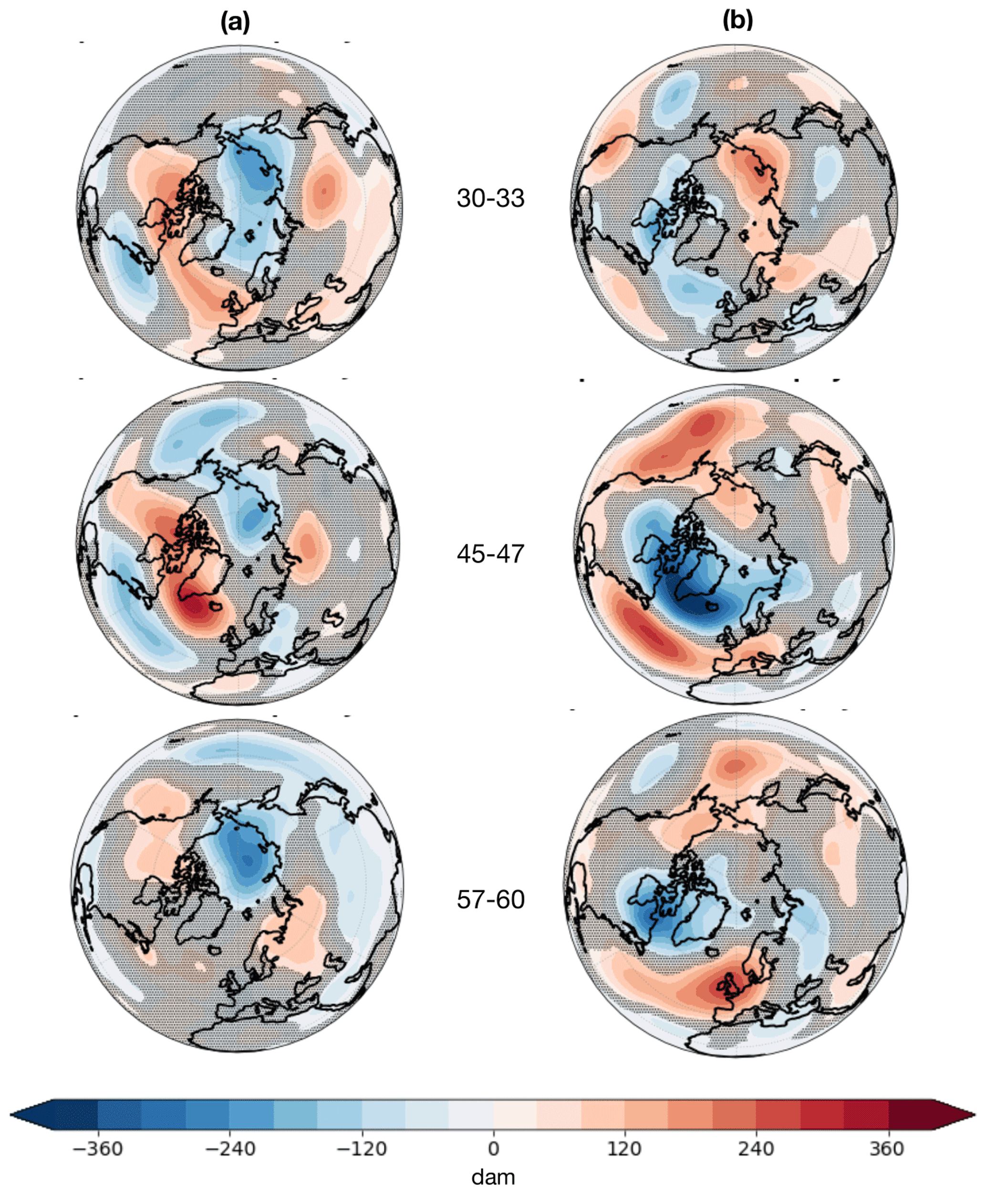
Figure 12Same as in Fig. 11, for DJF.
Table 1Sample sizes for extremes in each of the latitudinal circles chosen for the composite mean maps in Figs. 11 and 12.

JJA equatorward extremes are particularly interesting, given that they account for an a priori surprisingly large share of energy transport from the pole toward the Equator. As shown in Fig. 11, lower-latitude extremes are associated with widespread negative z500 anomalies, both on the main ocean basins and on land. This is consistent with a mainly equatorward energy transport. For higher-latitude extremes, a Euro-Scandinavian blocking pattern emerges, consistent with an increasing frequency of the EATC2 pattern, with negative z500 anomalies confined at even higher latitudes, and a dominant k = 2–3 wavenumber pattern. An interpretation of these features is provided in light of what described above (cf. Figs. 8 and 10). At lower latitudes (30–33∘ N), the increased likelihood of the PACC4 regime is consistent with co-located negative anomalies, especially over the Pacific, and a dominant k=4 wave. Overall, this hints at the role of the planetary-scale contribution, which is particularly relevant when the synoptic contribution is weak, especially at higher latitudes, where the planetary-to-total ratio is positive, as seen in Figs. 4 and 6. Looking at the composites, we interpret this equatorward or very weak poleward transport associated with equatorward extremes as the result of planetary-scale transport acting to confine baroclinic eddies in the high latitudes and overwhelming the synoptic-scale transport.
JJA poleward extremes also find a relatively straightforward interpretation in the z500 composites. For extremes located in the 30–33∘ N band, widespread negative z500 anomalies are found (although with very different patterns compared to the equatorward extremes), while at higher latitudes several blocking patterns emerge in the channel. Overall, the regime frequency changes (in particular the reduced frequency of the EATC4, PACC4 and NHC3 regimes) are consistent with this pattern, with the mid-latitudinal negative anomalies being replaced by co-located high-geopotential ridges. Consistent with Fig. 10, evidencing that these patterns are dominated by wavenumbers k = 5–6, Kornhuber et al. (2020) find that these modes of the general circulation are associated with the development of co-located heat waves in the NH summer. We thus argue that heat waves may plausibly be related to the occurrence of extremely strong poleward meridional energy transports.
To heuristically test this hypothesis, we focus on poleward extreme transports in JJA for the year 2010, which was characterized by a number of concurrent heat waves developing in several regions of the NH mid-latitudinal band, especially central-eastern North America and Russia (Dole et al., 2011). Figure 13 shows analogous results to those shown in Figs. 8, 10 and 11 for JJA 2010 only. Extremes at the three chosen latitudinal bands are associated with a positive anomaly over eastern Europe and Russia, particularly significant in the 45–47∘ N latitudinal band. The composites are also consistent with an increased frequency of the EATC2 and NHC4 patterns (Fig. 13b), especially in the higher latitudinal bands. In addition to that, some frequency reductions that are not as relevant in the rest of the extreme-event population are found for EATC1, PACC1 and NHC1, pointing towards a reduced occurrence of a regime similar to a NAO+ pattern and of the so-called “Aleutinian Ridge”.
Kornhuber et al. (2020) interpreted the 2010 heat wave as a case of concomitant heat waves over several regions of the Northern Hemisphere, a consequence of quasi-resonant (QRA) amplification of stationary Rossby waves (Kornhuber et al., 2017; Petoukhov et al., 2013). They found that k = 5–7 were particularly favorable to the development of this pattern. Consistently, Fig. 13c shows that more frequent regimes in the energy transport extreme population are associated with dominant wavenumbers ranging between k=4 and k=6. It is not our aim to establish here a dynamical linkage between the proposed QRA mechanism and the JJA poleward transport extremes. We rather conjecture that the emergence of concurrent heat waves with a k = 4–6 pattern may coincide with the emergence of such zonally integrated eddy-driven transport extremes, which deserves further investigation. Overall, we argue that the 2010 event is “typical” of the more general circulation features associated with poleward meridional-energy-transport extremes in JJA. The fact that the 2010 event captures a rare yet typically persistent fluctuation in the summer atmospheric fields in Eurasia has been discussed by Galfi and Lucarini (2021) using large-deviation-theory arguments. Analogously to the 2010 Russian heat wave case, we also found (not shown) that the Mongolia Dzud event occurred in winter 2010 (Rao et al., 2015; Sternberg, 2018), which was characterized by intense and persistent cold outbreaks throughout central Asia (Galfi and Lucarini, 2021), Overall, the composite mean analysis points to extreme meridional heat transport events being linked to recurrent atmospheric circulation patterns, which would enable the study of such extreme events using a rigorous formalism borrowed from statistical mechanics.
Looking at DJF z500 composites (Fig. 12), we note that the three latitudinal bands are characterized by a NAO− pattern when poleward extremes are taken into account. In the Pacific–North American sector, a strong ridge emerges over the American continent, moving westward and strengthening at 45–47∘ N, before weakening at 57–60∘ N. The described pattern is consistent with what is found in Fig. 7, the NAO−, PT and AO weather regimes becoming more frequent for extremes at all latitudes. At the same time, the Pacific dipole structure is opposed by negative anomalies over the Arctic and the high latitudes, consistent with a reduction in high-latitudinal blockings over that region, as denoted by the decreased frequency of ALR and BR regimes. Composites are also consistent with k = 2–3 being the range of dominant wavenumbers for the DJF poleward extremes, as seen in Fig. 9, with a relatively weak dependence on the weather regime assigned to the extreme event under consideration. The pattern for DJF equatorward extremes is to a certain extent reversed with respect to poleward extremes, with a clear NAO+ footprint in the poleward half of the mid-latitudinal band, and an ALR-like pattern for extremes located in the 45–47∘ N band. This reflects the fact that the dominant k = 2–4 wavenumbers do not change for the two classes of extremes, no matter the regime to which the events are assigned (cf. Fig. 9). It is rather the amplitude of ultra-long planetary-scale waves, carrying energy from the Equator towards the pole for both poleward and equatorward meridional transport extremes (cf. Fig. 3c), that determines the strength and location of the overall baroclinic eddy activity. Overall, we find that the composite maps are a blend of different regional-scale weather regimes, with significant values roughly resembling the pattern emerging from the description of Fig. 7. Zonally integrated transport extremes, in this context, reflect local features of the general circulation that are recurring and are possibly interconnected by the dominance of ultra-long planetary-scale waves.
In DJF, planetary- and synoptic-scale transport extremes rarely co-occur (as already stressed in Lembo et al., 2019, and above in this work), and the planetary contribution to the extreme transport is less dependent on the median value of the transport than the synoptic contribution. In other words, in DJF the planetary-scale pattern, embedding smaller-scale eddies, is dominant almost everywhere except at lower latitudes, and the synoptic-scale contribution sharply weakens with the median transport as the latitude increases. Synoptic-scale eddies are thus modulated by the strength of the underlying dominant planetary wave, as clearly suggested by the z500 anomalies. In contrast, the strengths of the planetary- and synoptic-scale contributions are comparable in JJA. The pattern highlighted by the composite analysis is thus a blend of the two competing factors, with synoptic scales becoming dominant in central latitudes (for poleward extremes) or the two contributions canceling each other almost symmetrically at most latitudes, confining baroclinic activity where the extreme transports occur (for equatorward extremes).
Summarizing, the composite analysis illustrates qualitatively that the extremes in the overall transport are the result of the interference of high and low wavenumbers (see also the discussion in Messori and Czaja, 2014, and Messori et al., 2017, on this topic). Such interference occurs in different ways in the two seasons, with the planetary-scale waves generally determining the latitude and strength of the baroclinic activity but the relative role of the synoptic and planetary waves being very different at different latitudes. The minima and maxima of the planetary- and synoptic-scale transports are in fact located at the two edges of the mid-latitudinal band in DJF and at the center of the band in JJA (cf. Figs. 3c, d and 4c, d). The zonally integrated approach does not allow the phases of the most relevant waves to be identified, but we provided some qualitative arguments by comparing dominant wavenumbers, weather regimes and composite analysis. For instance, DJF poleward (equatorward) extremes are denoted by increased (decreased) frequency in NAO−, AO and PT regimes and decreased (increased) frequency of NAO+ and ALR regimes, which is also partly reflected in the z500 composite means in Fig. 12. This is suggestive of a specific phase of the k = 2–3 waves, shaping the synoptic-scale baroclinic activity in the population of extremes and determining the increased and decreased blocking frequencies denoted by differences in weather regime frequencies.
In this work, we analyze the zonally averaged meridional energy transports in the mid-latitudinal NH band for the DJF and JJA seasons in ERA5 Reanalysis. We decomposed the transports depending on their zonal wavenumbers and isolated four contributions: zonal mean (k=0), planetary scales (k = 1–5), synoptic scales (k = 6–10) and higher scales (k = 11–20). We applied an EVT-based selection methodology to isolate extreme meridional-energy-transport events, labeled as “poleward” when the transport is stronger than average and “equatorward” when it is weaker. We adopted a clustering algorithm for the z500 anomalies associated with meridional-energy-transport extremes, and we looked for dominant patterns and preferred wavenumbers as a function of the latitudes at which the extremes are detected.
We find that energy transport extremes emerge as a result of the growth of different wave types across the mid-latitudes, particularly synoptic and planetary scales depending on meridional location and season. Specifically, dominant patterns and preferred wavenumbers suggest that planetary scales determine the strength and meridional position of the synoptic-scale baroclinic activity with their amplitude, exhibiting significant seasonal differences. In DJF, they modulate the synoptic-scale activity, being generally stronger than all other smaller scales, while in JJA they chiefly interfere with the latter being of similar magnitude, either constructively (poleward extremes) or destructively (equatorward extremes). Notably, equatorward extremes feature mainly negative-signed planetary-scale transports north of 42∘ N.
Understanding meridional-energy-transport extremes is key to identifying mechanisms through which diabatic heating and temperature gradients are balanced. We demonstrated that some preferred circulation regimes favor extreme transports and that they reflect to some extent preferential modes of variability related to specific zonal wavenumbers. This has clear implications for high-latitude warming and cooling, as already stressed before regarding the influence of synoptic-scale eddy activity on Arctic weather (cf. Ruggieri et al., 2020) or dynamical patterns related to extreme near-surface temperatures over the Arctic (cf. Messori et al., 2018; Papritz, 2020).
The emergence of dominant zonal wavenumbers associated with extreme meridional energy transports also has implications for teleconnections. Investigations based on large-deviation theory have shown that persistent weather extremes are associated with very large-scale atmospheric features (Gálfi et al., 2019; Galfi and Lucarini, 2021; Gálfi et al., 2021). We emphasized here the similarity between our results and the concurrent emergence of heat waves across the Northern Hemisphere associated with a persistent k = 5–7 Rossby wave pattern, as found by Kornhuber et al. (2020). Our results underscore that the variability modes related to energy transport extremes are hemispheric in scale and suggest that regional features such as the NAO or PNA trigger co-variability in weather in remote regions (Thompson and Wallace, 1998; Branstator, 2002). This was not clear a priori as the zonally integrated approach we adopt here does not allow, in principle, the selection of recurrent localized extreme transports, linked to regionally constrained circulation patterns. Further, analyzing the aggregated effect of wave packets on meridional energy transports and how they manifest in terms of weather regimes provides a thermodynamic background to the concept of QRA (Petoukhov et al., 2013; Coumou et al., 2014; Kornhuber et al., 2017) for the development of weather extremes, potentially linking local events to anomalies in the general circulation. Indeed, Petoukhov et al. (2013) already stressed that a weakened zonal component of high-amplitude waves is associated with the QRA hypothesis. This does not exclude, however, that the QRA mechanism can be associated with extremely strong meridional energy transports. We consider the investigation of dynamical linkages between energy transports and temperature (and moisture) advection in the context of concurrent heat waves amplified by a QRA mechanism as a potentially relevant topic for future work.
Here, we estimate the extremal index with the aim to decluster the energy transport time series in order to accelerate the convergence of extreme-value statistics. The extremal index itself, however, contains valuable information related to the persistence of extreme states as it is the inverse of the mean cluster size of extremes (Coles et al., 2001). In future studies, one could concentrate more on the persistence of extreme (and non-extreme) events in meridional energy transport based on the extremal index. The persistence of individual states together with the local attractor dimension can be used as a dynamical proxy for the general circulation. This approach has already successfully been applied to dynamical features of the atmosphere (Faranda et al., 2017; Messori et al., 2021), but never, to the best of our knowledge, to thermodynamic features.
Finally, a possible outcome of this analysis, which is left for future work, is the study of meridional-energy-transport extremes, their zonal wavenumber decomposition and the underlying dynamical drivers in numerical climate simulations. Assessing the statistics of these events against reanalysis-based data would provide an important background for the study of the climate response to external forcing and how changing statistics in extreme events related to baroclinic eddies can affect future weather predictability in the mid-latitudes (cf. Scher and Messori, 2019).
Figures A1 and A2 show patterns of the first four EOFs for DJF and JJA, respectively. These have been used to obtain the fractional change in the PC mean described in Fig. B1.

Figure A1Patterns of the four leading EOFs for DJF: EAT (first row), NH (second), PAC (third).
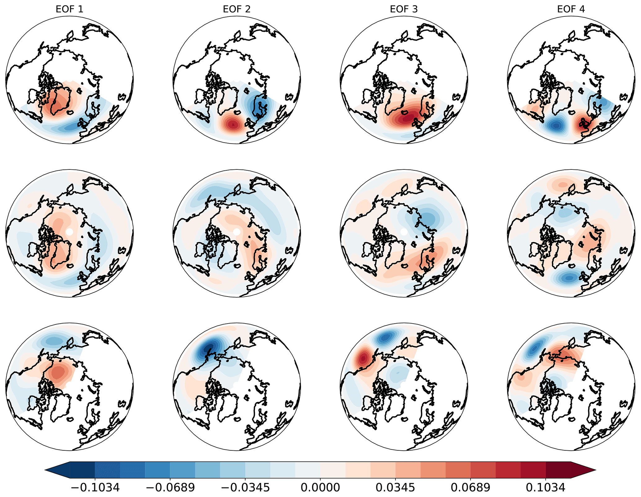
Figure A2Patterns of the four leading EOFs for JJA: EAT (first row), NH (second), PAC (third).
We investigate here changes in the PCs of the population of extremes, compared to the population of all days. For the sake of simplicity, we restrict ourselves to the four leading EOFs, computed in DJF and JJA over the three regions of interest: EAT, PAC and NH. Fractional changes in the mean of the PC distribution relative to the climatological standard deviation (Fig. B1) are evidenced when significant according to Welch's t test. We investigate shifts in the mean of the distribution in each dimension (PC), relative to the standard deviation of the climatological distribution.

Figure B1Fractional change (relative to climatological standard deviation) of the PC mean for the first four leading EOFs, as functions of the region of interest, for (a) DJF poleward extremes, (b) DJF equatorward extremes, (c) JJA poleward extremes and (d) JJA equatorward extremes. White dots denote the significance of the change with respect to the overall population of events. Large dots denote 99 % significance, and small dots denote 95 % significance.
In DJF, significant shifts are found for the first PC, corresponding to the positive phase of the Arctic Oscillation (AO) pattern for NH (Thompson and Wallace, 1998) and to the corresponding local patterns for EAT (NAO+) and PAC (Bering Ridge) (see Fig. A1 in Appendix A). Consistently, the distributions shift in opposite directions for equatorward and poleward transport extremes, respectively. The distribution of the third PCs (denoting a positive geopotential anomaly over the North Atlantic in EAT and over eastern Siberia in PAC) also change significantly in the population of equatorward extremes. In JJA, the most significant changes occur for higher-order EOFs, with the only exception of the poleward extremes in EAT, connected to the first EOF (NAO−). These higher-order EOFs are typically associated with localized patterns (e.g., EOF 3 and 4 for EAT and NH in Fig. A2), indicating that the extremes in this season are related to smaller scales of the circulation.
The choice of the threshold for the separation between planetary and synoptic scales, as well as the best indicator to consider the different scales, is the topic of an ongoing scientific discussion (Heiskanen et al., 2020; Stoll and Graversen, 2022). Here, we limit ourselves to testing an alternative wavenumber grouping, based on the available literature (e.g., Baggett and Lee, 2015; Shaw, 2014; Rydsaa et al., 2021). The same wavenumber might be identifying different types of motions at different latitudes (as discussed in Heiskanen et al., 2020, and Stoll and Graversen, 2022) such that a lower threshold may be appropriate at higher latitudes (e.g., k=3, Rydsaa et al., 2021; k=4, Shaw, 2014). Given that we analyze a relatively broad latitudinal band, our choice of k = 5 is a trade-off to provide a sensible length scale for the separation at different latitudes. Figure C1 shows the meridional-energy-transport PDFs for an alternative grouping, namely zonal wavenumbers k = 1–3, denoted as “ultra-long planetary waves”; k = 4–6, as “planetary waves”; and k = 7–9, as “synoptic waves”. The panel k = 0, i.e., zonal mean, is left unchanged. Starting from the DJF season (left panel), it is confirmed that ultra-long planetary waves are dominant, especially in the generation of “poleward” extremes at higher latitudes, whereas other planetary waves are relevant at all latitudes (with a roughly homogeneous contribution across latitudes). The contribution of synoptic waves is weaker than for the original choice of the wavenumber groups, although comparable to planetary waves, especially in the equatorward half of the mid-latitudinal band. Looking at JJA, the three eddy contributions are comparable, with planetary and synoptic waves mostly contributing to poleward extremes in the middle of the channel and ultra-long planetary waves contributing at lower and higher latitudes. Interestingly, ultra-long and planetary waves have a significant part of their PDFs related to equatorward extremes in the negative domain. In other words, we claim that both components transport energy “counter-gradient”, in opposition to the total transport. Overall, one might notice the following.
-
Synoptic-scale waves defined in this way are remarkably homogeneous across latitudes and seasons so that the only appreciable change is in the position of the peak. This is broadly coherent with our approach, considering k = 6–10 as the synoptic wave domain.
-
Ultra-long planetary waves play a dominant role in shaping the extremes in DJF, consistent with Figs. 7 and 9. Similarly, JJA extremes are characterized by the coexistence of comparable planetary and synoptic contributions, although the former still dominate poleward transports, while ultra-long waves hardly distinguish between poleward and equatorward extremes.
-
The regrouped wavenumbers support the conclusion that the strength of the extremes is in all cases dependent on the shape of the median meridional section. The k = 1–5 grouping showing no correlation with the median is the result of the latitudinally homogeneous median in the k = 4–6 range, plus the weaker contribution by ultra-long waves in low latitudes.

ERA5 Reanalysis data are publicly accessible via Copernicus Data Storage (https://doi.org/10.24381/cds.adbb2d47, Hersbach et al., 2018). The computation of meridional energy transport and its wavenumber decomposition was performed at the ECMWF data server and stored at the NIRD storage facility provided by the Norwegian e-infrastructure for research and education UNINETT Sigma2 under the project NS9063K. This can be accessed upon request to Rune Grand Graversen.
VLe, VLu and GM designed the analysis and wrote the manuscript. RG performed the wavenumber decomposition of meridional energy transports, VMG conceived the algorithm for extreme-event detection and carried out the convergence analysis, and FF performed the EOF and k-means clustering analysis and attribution of events. All authors contributed to the interpretation of the results.
The contact author has declared that none of the authors has any competing interests.
Publisher's note: Copernicus Publications remains neutral with regard to jurisdictional claims in published maps and institutional affiliations.
Gabriele Messori has received funding from the European Research Council (ERC) under the European Union's Horizon 2020 research and innovation program (grant agreement no. 948309, CENÆ project). Valerio Lucarini acknowledges the support received from the EPSRC project EP/T018178/1 and from the EU Horizon 2020 project TiPES (grant no. 820970). The work is also associated with the Norwegian Science Foundation (NFR) project no. 280727.
This research has been supported by the European Research Council (ERC) and a Research Innovation Action (RIA) under the European Union’s Horizon 2020 research and innovation program (grant nos. 948309 and 820970) and the Norwegian Science Foundation (NFR; project no. 280727).
This paper was edited by Pedram Hassanzadeh and reviewed by two anonymous referees.
Ambaum, M. H. P.: Thermal Physics of the Atmosphere, Wiley-Blackwell, https://doi.org/10.1002/9780470710364, 2010. a
Baggett, C. and Lee, S.: Arctic Warming Induced by Tropically Forced Tapping of Available Potential Energy and the Role of the Planetary-Scale Waves, J. Atmos. Sci., 72, 1562–1568, https://doi.org/10.1175/JAS-D-14-0334.1, 2015. a, b, c, d
Balkema, A. A. and de Haan, L.: Residual Life Time at Great Age, Ann. Probab., 2, 792–804, https://doi.org/10.1214/aop/1176996548, 1974. a
Barnes, E. A. and Polvani, L.: Response of the midlatitude jets, and of their variability, to increased greenhouse gases in the CMIP5 models, J. Climate, 26, 7117–7135, 2013. a
Boisvert, L. and Stroeve, J. C.: The Arctic is becoming warmer and wetter as revealed by the Atmospheric Infrared Sounder, Geophys. Res. Lett., 42, 4439–4446, 2015. a
Bowman, A. W. and Azzalini, A.: Applied smoothing techniques for data analysis: the kernel approach with S-Plus illustrations, vol. 18, OUP Oxford, https://doi.org/10.1007/s001800000033, 1997. a
Branstator, G.: Circumglobal teleconnections, the jet stream waveguide, and the North Atlantic Oscillation, J. Climate, 15, 1893–1910, 2002. a
Cassou, C.: Intraseasonal interaction between the Madden–Julian Oscillation and the North Atlantic Oscillation, Nature, 455, 523–527, https://doi.org/10.1038/nature07286, 2008. a, b, c
Cattiaux, J., Douville, H., and Peings, Y.: European temperatures in CMIP5: origins of present-day biases and future uncertainties, Clim. Dynam., 41, 2889–2907, 2013. a
Coles, S., Bawa, J., Trenner, L., and Dorazio, P.: An introduction to statistical modeling of extreme values, vol. 208, Springer, https://doi.org/10.1007/978-1-4471-3675-0, 2001. a, b, c, d
Corti, S., Molteni, F., and Palmer, T. N.: Signature of recent climate change in frequencies of natural atmospheric circulation regimes, Nature, 398, 799–802, https://doi.org/10.1038/19745, 1999. a
Coumou, D., Petoukhov, V., Rahmstorf, S., Petri, S., and Schellnhuber, H. J.: Quasi-resonant circulation regimes and hemispheric synchronization of extreme weather in boreal summer, P. Natl. Acad. Sci. USA, 111, 12331–12336, 2014. a
Dawson, A., Palmer, T. N., and Corti, S.: Simulating regime structures in weather and climate prediction models, Geophys. Res. Lett., 39, L21805, https://doi.org/10.1029/2012GL053284, 2012. a, b
Dole, R., Hoerling, M., Perlwitz, J., Eischeid, J., Pegion, P., Zhang, T., Quan, X.-W., Xu, T., and Murray, D.: Was there a basis for anticipating the 2010 Russian heat wave?, Geophys. Res. Lett., 38, https://doi.org/10.1029/2010GL046582, 2011. a, b
Dorrington, J., Strommen, K., and Fabiano, F.: Quantifying climate model representation of the wintertime Euro-Atlantic circulation using geopotential-jet regimes, Weather Clim. Dynam., 3, 505–533, https://doi.org/10.5194/wcd-3-505-2022, 2022. a
Dufour, A., Zolina, O., and Gulev, S. K.: Atmospheric moisture transport to the Arctic: Assessment of reanalyses and analysis of transport components, J. Climate, 29, 5061–5081, 2016. a
Fabiano, F., Christensen, H., Strommen, K., Athanasiadis, P., Baker, A., Schiemann, R., and Corti, S.: Euro-Atlantic weather Regimes in the PRIMAVERA coupled climate simulations: impact of resolution and mean state biases on model performance, Clim. Dynam., 54, 5031–5048, 2020. a, b
Fabiano, F., Meccia, V. L., Davini, P., Ghinassi, P., and Corti, S.: A regime view of future atmospheric circulation changes in northern mid-latitudes, Weather Clim. Dynam., 2, 163–180, https://doi.org/10.5194/wcd-2-163-2021, 2021. a, b
Faranda, D., Messori, G., Alvarez-Castro, M. C., and Yiou, P.: Dynamical properties and extremes of Northern Hemisphere climate fields over the past 60 years, Nonlin. Processes Geophys., 24, 713–725, https://doi.org/10.5194/npg-24-713-2017, 2017. a, b
Ferro, C. A. T. and Segers, J.: Inference for Clusters of Extreme Values, J. R. Stat. Soc. B, 65, 545–556, http://www.jstor.org/stable/3647520 (last access: 24 November 2021), 2003. a
Forthofer, R. N. and Lehnen, R. G.: Rank Correlation Methods, in: Public Program Analysis, Springer, Boston, MA, 146–163, https://doi.org/10.1007/978-1-4684-6683-6_9, 1981. a
Freedman, D. and Diaconis, P.: On the histogram as a density estimator: L2 theory, Z. Wahrscheinlichkeit., 57, 453–476, 1981. a
Galfi, V. M. and Lucarini, V.: Fingerprinting Heatwaves and Cold Spells and Assessing Their Response to Climate Change Using Large Deviation Theory, Phys. Rev. Lett., 127, 058701, https://doi.org/10.1103/PhysRevLett.127.058701, 2021. a, b, c, d
Gálfi, V. M., Bódai, T., and Lucarini, V.: Convergence of extreme value statistics in a two-layer quasi-geostrophic atmospheric model, Complexity, 2017, 5340858, https://doi.org/10.1155/2017/5340858, 2017. a, b
Gálfi, V. M., Lucarini, V., and Wouters, J.: A large deviation theory-based analysis of heat waves and cold spells in a simplified model of the general circulation of the atmosphere, J. Stat. Mech. Theory E., 3, 033404, https://doi.org/10.1088/1742-5468/ab02e8, 2019. a
Gálfi, V. M., Lucarini, V., Ragone, F., and Wouters, J.: Applications of large deviation theory in geophysical fluid dynamics and climate science, Riv Nuovo Cimento, 44, 291–363, https://doi.org/10.1007/s40766-021-00020-z, 2021. a
Gnedenko, B.: Sur la distribution limite du terme maximum d'une serie aleatoire, Ann. Math., 44, 423–453, 1943. a
Graversen, R. G. and Burtu, M.: Arctic amplification enhanced by latent energy transport of atmospheric planetary waves, Q. J. Roy. Meteor. Soc., 142, 2046–2054, 2016. a, b, c, d, e, f
Guemas, V., Salas-Mélia, D., Kageyama, M., Giordani, H., Voldoire, A., and Sanchez-Gomez, E.: Summer interactions between weather regimes and surface ocean in the North-Atlantic region, Clim. Dynam., 34, 527–546, https://doi.org/10.1007/s00382-008-0491-6, 2010. a
Hannachi, A., Straus, D. M., Franzke, C. L. E., Corti, S., and Woollings, T.: Low-frequency nonlinearity and regime behavior in the Northern Hemisphere extratropical atmosphere, Rev. Geophys., 55, 199–234, https://doi.org/10.1002/2015RG000509, 2017. a
Heiskanen, T., Graversen, R. G., Rydsaa, J. H., and Isachsen, P. E.: Comparing wavelet and Fourier perspectives on the decomposition of meridional energy transport into synoptic and planetary components, Q. J. Roy. Meteor. Soc., 146, 2717–2730, https://doi.org/10.1002/QJ.3813, 2020. a, b, c, d, e, f
Hersbach, H., Bell, B., Berrisford, P., Biavati, G., Horányi, A., Muñoz Sabater, J., Nicolas, J., Peubey, C., Radu, R., Rozum, I., Schepers, D., Simmons, A., Soci, C., Dee, D., and Thépaut, J.-N.: ERA5 hourly data on single levels from 1959 to present, Copernicus Climate Change Service (C3S) Climate Data Store (CDS) [data set], https://doi.org/10.24381/cds.adbb2d47, 2018. a, b
Hersbach, H., Bell, B., Berrisford, P., Hirahara, S., Horányi, A., Muñoz-Sabater, J., Nicolas, J., Peubey, C., Radu, R., Schepers, D., Simmons, A., Soci, C., Abdalla, S., Abellan, X., Balsamo, G., Bechtold, P., Biavati, G., Bidlot, J., Bonavita, M., De Chiara, G., Dahlgren, P., Dee, D., Diamantakis, M., Dragani, R., Flemming, J., Forbes, R., Fuentes, M., Geer, A., Haimberger, L., Healy, S., Hogan, R. J., Hólm, E., Janisková, M., Keeley, S., Laloyaux, P., Lopez, P., Lupu, C., Radnoti, G., de Rosnay, P., Rozum, I., Vamborg, F., Villaume, S., and Thépaut, J.-N.: The ERA5 global reanalysis, Q. J. Roy. Meteor. Soc., 146, 1999–2049, 2020. a
Hochman, A., Messori, G., Quinting, J. F., Pinto, J. G., and Grams, C. M.: Do Atlantic-European weather regimes physically exist?, Geophys. Res. Lett., 48, e2021GL095574, https://doi.org/10.1029/2021GL095574, 2021. a
Holton, J. R. and Hakim, G. J.: An Introduction to Dynamic Meteorology, Academic Press, 552 pp., ISBN 9780123848666, 2012. a
Hwang, Y.-T., Frierson, D. M., and Kay, J. E.: Coupling between Arctic feedbacks and changes in poleward energy transport, Geophys. Res. Lett., 38, L17704, https://doi.org/10.1029/2011GL048546, 2011. a
Jung, T., Palmer, T. N., and Shutts, G. J.: Influence of a stochastic parameterization on the frequency of occurrence of North Pacific weather regimes in the ECMWF model, Geophys. Res. Lett., 32, L23811, https://doi.org/10.1029/2005GL024248, 2005. a
Kaspi, Y. and Schneider, T.: The role of stationary eddies in shaping midlatitude storm tracks, J. Atmos. Sci., 70, 2596–2613, 2013. a
Kimoto, M. and Ghil, M.: Multiple Flow Regimes in the Northern Hemisphere Winter. Part I: Methodology and Hemispheric Regimes, J. Atmos. Sci., 50, 2625–2644, https://doi.org/10.1175/1520-0469(1993)050<2625:MFRITN>2.0.CO;2, 1993. a
Kornhuber, K., Petoukhov, V., Petri, S., Rahmstorf, S., and Coumou, D.: Evidence for wave resonance as a key mechanism for generating high-amplitude quasi-stationary waves in boreal summer, Clim. Dynam., 49, 1961–1979, 2017. a, b
Kornhuber, K., Coumou, D., Vogel, E., Lesk, C., Donges, J. F., Lehmann, J., and Horton, R. M.: Amplified Rossby waves enhance risk of concurrent heatwaves in major breadbasket regions, Nat. Clim. Change, 10, 48–53, 2020. a, b, c
Leadbetter, M., Weissman, I., De Haan, L., and Rootzén, H.: On clustering of high values in statistically stationary series, Proc. 4th Int. Meet. Statistical Climatology, Rotorua, New Zealand, 27–31 March 1989, edited by: Sanson, J., New Zealand Meteorological Service, Wellington, New Zealand, 1989. a
Leadbetter, M. R.: On extreme values in stationary sequences, Z. Wahrscheinlichkeit., 28, 289–303, 1974. a, b
Lembo, V., Messori, G., Graversen, R. G., and Lucarini, V.: Spectral Decomposition and Extremes of Atmospheric Meridional Energy Transport in the Northern Hemisphere Midlatitudes, Geophys. Res. Lett., 46, 2019GL082105, https://doi.org/10.1029/2019GL082105, 2019. a, b, c, d, e, f, g, h, i, j, k
Liang, M., Czaja, A., Graversen, R., and Tailleux, R.: Poleward energy transport: is the standard definition physically relevant at all time scales?, Clim. Dynam., 50, 1785–1797, https://doi.org/10.1007/S00382-017-3722-X, 2017. a
Liu, C. and Barnes, E. A.: Extreme moisture transport into the Arctic linked to Rossby wave breaking, J. Geophys. Res.-Atmos., 120, 3774–3788, 2015. a
Lorenz, E. N.: Available Potential Energy and the Maintenance of the General Circulation, Tellus, 7, 157–167, https://doi.org/10.1111/j.2153-3490.1955.tb01148.x, 1955. a
Lorenz, E. N.: The nature and theory of the general circulation of the atmosphere, vol. 218, World Meteorological Organization, Geneva, https://library.wmo.int/index.php?lvl=notice_display&id=5571 (last access: 5 September 2022), 1967. a
Lucarini, V. and Ragone, F.: Energetics of Climate Models: Net Energy Balance and Meridional Enthalpy Transport, Rev. Geophys., 49, RG1001, https://doi.org/10.1029/2009RG000323, 2011. a
Mann, H.: Nonparametric tests against trend, Econometrica, 13, 245–259, 1945. a
Marcheggiani, A., Ambaum, M. H., and Messori, G.: The life cycle of meridional heat flux peaks, Q. J. Roy. Meteor. Soc., 148, 1113–1126, 2022. a
Messori, G. and Czaja, A.: On the sporadic nature of meridional heat transport by transient eddies, Q. J. Roy. Meteor. Soc., 139, 999–1008, 2013. a, b
Messori, G. and Czaja, A.: Some considerations on the spectral features of meridional heat transport by transient eddies, Q. J. Roy. Meteor. Soc., 140, 1377–1386, 2014. a, b
Messori, G. and Czaja, A.: On local and zonal pulses of atmospheric heat transport in reanalysis data, Q. J. Roy. Meteor. Soc., 141, 2376–2389, 2015. a, b, c, d
Messori, G., Geen, R., and Czaja, A.: On the spatial and temporal variability of atmospheric heat transport in a hierarchy of models, J. Atmos. Sc., 74, 2163–2189, 2017. a, b
Messori, G., Woods, C., and Caballero, R.: On the drivers of wintertime temperature extremes in the high Arctic, J. Climate, 31, 1597–1618, 2018. a
Messori, G., Harnik, N., Madonna, E., Lachmy, O., and Faranda, D.: A dynamical systems characterization of atmospheric jet regimes, Earth Syst. Dynam., 12, 233–251, https://doi.org/10.5194/esd-12-233-2021, 2021. a
Michelangeli, P.-A., Vautard, R., and Legras, B.: Weather Regimes: Recurrence and Quasi Stationarity, J. Atmos. Sci., 52, 1237–1256, https://doi.org/10.1175/1520-0469(1995)052<1237:WRRAQS>2.0.CO;2, 1995. a
Moon, W., Manucharyan, G. E., and Dijkstra, H. A.: Baroclinic instability and large-scale wave propagation in a planetary-scale atmosphere, Q. J. Roy. Meteor. Soc., 148, 809–825, 2022. a
Nie, J., Wang, P., Yang, W., and Tan, B.: Northern Hemisphere storm tracks in strong AO anomaly winters, Atmos. Sci. Lett., 9, 153–159, https://doi.org/10.1002/ASL.186, 2008. a
Novak, L., Ambaum, M. H. P., and Tailleux, R.: The Life Cycle of the North Atlantic Storm Track, J. Atmos. Sci., 72, 821–833, https://doi.org/10.1175/JAS-D-14-0082.1, 2015. a, b
Papritz, L.: Arctic lower-tropospheric warm and cold extremes: Horizontal and vertical transport, diabatic processes, and linkage to synoptic circulation features, J. Climate, 33, 993–1016, 2020. a
Pasquier, J., Pfahl, S., and Grams, C. M.: Modulation of atmospheric river occurrence and associated precipitation extremes in the North Atlantic region by European weather regimes, Geophys. Res. Lett., 46, 1014–1023, 2019. a
Peixoto, J. P. and Oort, A. H.: Physics of climate, American Institute of Physics, New York, NY, USA, ISBN 978-0-88318-712-8, 1992. a
Petoukhov, V., Rahmstorf, S., Petri, S., and Schellnhuber, H. J.: Quasiresonant amplification of planetary waves and recent Northern Hemisphere weather extremes, P. Natl. Acad. Sci. USA, 110, 5336–5341, 2013. a, b, c
Pickands, J. I.: Statistical Inference Using Extreme Order Statistics, Ann. Stat., 3, 119–131, https://doi.org/10.1214/aos/1176343003, 1975. a
Rao, M. P., Davi, N., Arrigo, R., Skees, J., Baatarbileg, N., Leland, C., Lyon, B., Wang, S.-Y., and Byambasuren, O.: Dzuds, droughts, and livestock mortality in Mongolia, Environ. Res. Lett., 10, 074012, https://doi.org/10.1088/1748-9326/10/7/074012, 2015. a
Ruggieri, P., Alvarez-Castro, M. C., Athanasiadis, P., Bellucci, A., Materia, S., and Gualdi, S.: North Atlantic circulation regimes and heat transport by synoptic eddies, J. Climate, 33, 4769–4785, https://doi.org/10.1175/JCLI-D-19-0498.1, 2020. a, b
Rydsaa, J. H., Graversen, R., Heiskanen, T. I. H., and Stoll, P.: Changes in atmospheric latent energy transport into the Arctic: Planetary versus synoptic scales, Q. J. Roy. Meteor. Soc., 147, 2281–2292, 2021. a, b, c, d
Scher, S. and Messori, G.: How Global Warming Changes the Difficulty of Synoptic Weather Forecasting, Geophys. Res. Lett., 46, 2931–2939, https://doi.org/10.1029/2018GL081856, 2019. a
Shaw, T. A.: On the role of planetary-scale waves in the abrupt seasonal transition of the Northern Hemisphere general circulation, J. Atmos. Sc., 71, 1724–1746, 2014. a, b
Skific, N. and Francis, J. A.: Drivers of projected change in Arctic moist static energy transport, J. Geophys. Res.-Atmos., 118, 2748–2761, 2013. a
Starr, V. and White, R.: Balance Requirements of the General Circulation, Tech. rep., Air Force Research Center, Cambridge, MA, https://apps.dtic.mil/sti/citations/AD0059398 (last access: 23 December 2021), 1954. a
Sternberg, T.: Investigating the presumed causal links between drought and dzud in Mongolia, Nat. Hazards, 92, 27–43, https://doi.org/10.1007/s11069-017-2848-9, 2018. a
Stoll, P. J. and Graversen, R. G.: The global atmospheric energy transport analysed by a wavelength-based scale separation, Weather Clim. Dynam. Discuss. [preprint], https://doi.org/10.5194/wcd-2022-26, in review, 2022. a, b, c, d, e
Straus, D. M., Molteni, F., and Corti, S.: Atmospheric Regimes: The Link between Weather and the Large-Scale Circulation, Cambridge University Press, https://doi.org/10.1017/9781316339251.005, 105–135, 2017. a, b, c
Strommen, K., Mavilia, I., Corti, S., Matsueda, M., Davini, P., von Hardenberg, J., Vidale, P.-L., and Mizuta, R.: The Sensitivity of Euro-Atlantic Regimes to Model Horizontal Resolution, Geophys. Res. Lett., 46, 7810–7818, https://doi.org/10.1029/2019GL082843, 2019. a
Swanson, K. L. and Pierrehumbert, R. T.: Lower-tropospheric heat transport in the Pacific storm track, J. Atmos. Sci., 54, 1533–1543, 1997. a
Thompson, D. W. and Wallace, J. M.: The Arctic Oscillation signature in the wintertime geopotential height and temperature fields, Geophys. Res. Lett., 25, 1297–1300, 1998. a, b
Tolstov, G. P.: Fourier series, Courier Corporation, ISBN 978-0133299380, 2012. a
Weisheimer, A., Corti, S., Palmer, T., and Vitart, F.: Addressing model error through atmospheric stochastic physical parametrizations: impact on the coupled ECMWF seasonal forecasting system, Philos. T. R. Soc. A, 372, 20130290, https://doi.org/10.1098/RSTA.2013.0290, 2014. a, b
White, R. H., Kornhuber, K., Martius, O., and Wirth, V.: From Atmospheric Waves to Heatwaves: A Waveguide Perspective for Understanding and Predicting Concurrent, Persistent, and Extreme Extratropical Weather, B. Am. Meteorol. Soc., 103, E923–E935, https://doi.org/10.1175/BAMS-D-21-0170.1, 2022. a
Woods, C., Caballero, R., and Svensson, G.: Large-scale circulation associated with moisture intrusions into the Arctic during winter, Geophys. Res. Lett., 40, 4717–4721, 2013. a
Yiou, P., Malamud, B. D., and Rust, H. W.: Preface “Extreme Events: Nonlinear Dynamics and Time Series Analysis”, Nonlin. Processes Geophys., 18, 895–897, https://doi.org/10.5194/npg-18-895-2011, 2011. a
The asymptotic GPD shape parameter is not affected by the existence of clusters; its finite-size estimates however are biased due to the slow convergence.
- Abstract
- Introduction
- Methodology
- Results
- Discussion
- Summary and conclusions
- Appendix A: EOF patterns for k-means clusters selection
- Appendix B: Shifts in the extreme-event PCs
- Appendix C: Energy transport PDFs for different choices of planetary wave threshold
- Data availability
- Author contributions
- Competing interests
- Disclaimer
- Acknowledgements
- Financial support
- Review statement
- References