Recurrent Rossby waves and south-eastern Australian heatwaves

In the Northern Hemisphere, recurrence of transient synoptic-scale Rossby wave packets in the same phase over periods of days to weeks, termed RRWPs, may repeatedly create similar surface weather conditions. This recurrence can lead to persistent surface anomalies. Here, we first demonstrate the significance of RRWPs for persistent hot spells in the Southern Hemisphere (SH) using the ERA-Interim (ERA-I) reanalysis dataset and then examine the role of RRWPs and blocks for heatwaves over south-eastern Australia (SEA).

A Weibull regression analysis shows that RRWPs are statistically associated with a significant increase in the duration of hot spells over several regions in the SH, including SEA. Two case studies of heatwaves in SEA in the summers of 2004 and 2009 illustrate the role of RRWPs in forming recurrent ridges (anticyclonic potential vorticity – PV – anomalies), aiding in the persistence of the heatwaves. Then, using a weather-station-based dataset to identify SEA heatwaves, we find that SEA heatwaves are more frequent than climatology during days with extreme RRWPs activity over SEA (high R_SEA). On days with both high R_SEA and heatwaves, circumglobal zonal wavenumber 4 and 5 (WN4, WN5) anomaly patterns are present in the composite mean of the upper-level PV field, with an anticyclonic PV anomaly over SEA. The Fourier decomposition of the PV and meridional wind velocity fields further reveals that the WN4 and WN5 components in the suitable phase aids in forming the ridge over SEA for days with high R_SEA. In addition, we find anomalous blocking over the Indian and the South Pacific oceans during SEA heatwaves, which may help to modulate the phase of RRWPs.

1 Introduction

Since 1900, extreme heat has been responsible for more fatalities in Australia than all other natural hazards combined (Coates et al., 2014). Heatwaves also exacerbate the risk of wildfires, cause surges in power demand, and increase insurance costs (Hughes et al., 2020; Insurance Council of Australia, 2020). Increasingly frequent and severe heatwaves in the midlatitudes in the recent years (Coumou et al., 2013; Perkins-Kirkpatrick and Lewis, 2020; IPCC, 2021) have spurred fruitful research on the atmospheric drivers of heatwaves. Understanding the dynamical mechanisms is particularly important for improving sub-seasonal prediction (Quandt et al., 2017) and for quantifying future changes in heatwaves (Shepherd, 2014; Wehrli et al., 2019).

Several large-scale atmospheric mechanisms and phenomena have been identified as potential drivers of heatwaves in the Northern Hemisphere (NH) extratropics. They include blocking anticyclones (e.g. Barriopedro et al., 2011; Drouard and Woollings, 2018; Kautz et al., 2022), amplified quasi-stationary waves (Teng et al., 2016; Kornhuber et al., 2017), amplified Rossby wave packets (e.g. Fragkoulidis et al., 2018; Kornhuber et al., 2020), and recurrent Rossby wave packets (Röthlisberger et al., 2019). Fragkoulidis et al. (2018) showed that amplified Rossby waves are correlated with surface temperature extremes over NH and used process-based understanding to establish further association for the 2003 and 2010 NH heatwaves.

RRWPs can be considered a subset of amplified Rossby waves with a condition that the transient eddies recur spatially in the same phase on a short timescale of days to weeks. RRWPs are closely related to blocking. RRWPs forming upstream of a block can sustain the block (e.g. Shutts, 1983; Hoskins et al., 1985; Hoskin and Sardeshmukh, 1987). RRWPs can also form downstream of blocks because of the near-constant phase of the wave breaking (trough) on the downstream flank of the blocks (Barton et al., 2016; Röthlisberger et al., 2018). Here, we focus on recurrent Rossby wave packets to explore their importance for heatwaves in south-eastern Australia (SEA).

Broadly, heatwaves in SEA (Fig. 1), comprising the states of Victoria (VIC), New South Wales (NSW), South Australia (SA), and Tasmania (TAS), are associated with slow-moving transient anticyclonic upper-level potential vorticity (PV) anomalies over the Tasman Sea (e.g. Marshall et al., 2014; Parker et al., 2014b; Quinting and Reeder, 2017; Parker et al., 2020). The anticyclonic PV anomalies and the associated subsidence drive heatwaves over VIC (Parker et al., 2014b; Quinting and Reeder, 2017). These anticyclonic PV anomalies can form as part of a synoptic-scale Rossby wave packet (RWP) (King and Reeder, 2021). These RWPs are often initiated several days before the onset of the heatwaves, but they amplify and eventually break anticyclonically over SEA (Parker et al., 2014b; O'Brien and Reeder, 2017).

Figure 1 Map of Australia showing the states of south-eastern Australia (SEA): South Australia (SA), Tasmania (TAS), Victoria (VIC), and New South Wales (NSW). Other states shown are Queensland (QLD), Northern Territory (NT), and Western Australia (WA). Red dots indicate the Australian Bureau of Meteorology's (BoM) monitoring stations used in this study (see Sect. 2).

Surface temperature anomalies associated with transient RWPs form, amplify, and decay on synoptic timescales, but the recurrence of RWPs in the same phase on a sub-seasonal timescale can result in persistent surface weather conditions by repeatedly re-enforcing the surface temperature anomalies (e.g. Hoskins and Sardeshmukh, 1987; Davies, 2015). Röthlisberger et al. (2019) termed this phenomenon “recurrent Rossby wave packets” (RRWPs) and demonstrated a statistically significant connection between RRWPs and the persistence of surface temperature anomalies in the Northern Hemisphere (NH). Ali et al. (2021) found that RRWPs are also associated with increased persistence of dry and wet spells in several regions across the globe.

For some impacts, however, it is not only the simple occurrence of an extreme that defines an extreme but also the duration of the extreme event that is important. This study addresses that aspect for the hot temperature extremes in the SH. More precisely, we evaluate the hypothesis whether an increase in the R metric, a measure of RRWPs (Röthlisberger et al., 2019), is associated with an increase in hot-spell duration of the surface temperature extremes over SH. Furthermore, we show how SH RRWPs relate to the persistent and extreme SEA heatwaves and demonstrate their association with RRWPs and atmospheric blocking the help of two case studies for the 2004 and 2009 heatwaves.

2 Methods

2.1 Data

This study uses ERA-Interim (ERA-I) reanalysis data (Dee et al., 2011) provided by the European Centre for Medium-Range Weather Forecasts on a $\mathrm{1}{}^{\circ }\times \mathrm{1}{}^{\circ }$ spatial grid and 6-hourly temporal resolution for 1979–2018. The datasets used are meridional wind velocity, 2 m temperature (T2m), and PV. Daily-maximum 2 m temperature is derived from T2m data, and the anomalies in daily-maximum T2m data are calculated with respect to the day-of-year mean for the period 1979–2018. The datasets are freely available to download from https://apps.ecmwf.int/datasets/data/interim-full-daily/levtype=pl/ (last access: 25 September 2019). PV fields are used as it is for calculating the blocking fields. However, for rest of the analysis, the PV fields are multiplied by minus one, which implies that negative (positive) PV anomalies represent anticyclones (cyclones) similar to the NH.

2.2 Recurrent Rossby waves

The R metric, developed by Röthlisberger et al. (2019), is used to quantify the recurrence of synoptic-scale Rossby wave packets. For the SH, we use the same R-metric data as in Ali et al. (2021). First, 6-hourly meridional winds at 250 hPa are averaged between 35 and 65^∘ S as v_ma(λ,t). To the resulting longitude–time data v_ma(λ,t), a 14.25 d (day) running mean, is applied to isolate signals with timescales longer than the synoptic timescale. This results in a longitude–time field of temporally smoothed, meridionally averaged 250 hPa meridional wind v_tf(λ,t). The envelope of the synoptic wavenumber contribution to the time-filtered v_tf(λ,t) is extracted following Zimin et al. (2003) as follows: the v_tf(λ,t) is transformed into the frequency domain for each t using a fast Fourier transform over longitude, yielding Fourier coefficients ${\widehat{v}}_{\mathrm{tf}}(k,t)$ for zonal wavenumber k at the time step t. Finally, an inverse Fourier transform is applied to calculate the envelope of the wave while only considering contributions from a selected band of synoptic wavenumbers k= 4–15. Thus, R(λ,t) for each longitude λ and time t is calculated as

$$\begin{array}{}\text{(1)}& R(\mathit{\lambda },t)=\left|\mathrm{2}\sum _{k=\mathrm{4}}^{k=\mathrm{15}}{\widehat{v}}_{\mathrm{tf}}(k,t)e^{\mathrm{2}\mathit{\pi }ik{l}_{\mathit{\lambda }}/N}\right|,\end{array}$$

where k is the wavenumber, l_λ denotes the longitudinal grid point index for longitude λ, and N=360 denotes the number of longitudinal grid points.

In most cases, large values of R reliably identify situations in which amplified waves (of distinct wave packets) recur in the same phase. However, the definition of R does not contain a criterion for recurrence of distinct wave packets. Thus, in a few cases, high values of R over a few days may result from stationary synoptic-scale troughs or ridges (see Röthlisberger et al., 2019, for a discussion on the R metric). Figure A1 shows the day-of-year climatology of the R metric in the Southern Hemisphere and compares it to that of the Northern Hemisphere. The code for calculating the R metric is freely available (see “Code and data availability”).

For the phase–amplitude information used in Sect. 3.3, it is extracted using the Fourier decomposition along the longitude of meridionally averaged (35 and 65^∘ S) 250 hPa meridional wind v_ma(λ,t) as used for calculating the R metric above. After applying the fast Fourier transform, one obtains Fourier coefficients in the form of complex numbers $\widehat{v}(k,t)$. Plotting the complex number on a complex plane, i.e. real vs. imaginary (Img) axis, provides information on the phase and amplitude at a given time step t for a particular wavenumber k.

2.3 Atmospheric blocks

Atmospheric blocking data are computed following the methodology of Schwierz et al. (2004) as in Rohrer et al. (2020) and Lenggenhager and Martius (2019). The detection scheme identifies persistent anticyclonic PV anomalies vertically averaged (VAPV) between 500 and 150 hPa vertical levels. First, the VAPV anomaly is computed from the 30 d running mean climatology of the corresponding time step of the year for the years 1979–2018. An additional 2 d running mean filter is applied to smooth out high-frequency transients. Then the algorithm identifies areas with VAPV ≥1.3 PVU (potential vorticity unit) in the SH. The identified areas having a persistence criterion of 5 d and a minimum overlap of 0.7 between consecutive time steps are classified as blocks. Blocking fields identified with this algorithm are available at 6-hourly temporal resolution and $\mathrm{1}{}^{\circ }\times \mathrm{1}{}^{\circ }$ spatial resolution. We tested the blocking fields with a less stringent threshold of VAPV ≥1.0 PVU for the two case studies and did not find blocking directly over SEA. The code used to calculate blocks is available on GitHub (see “Code and data availability”).

2.4 South-eastern Australian heatwaves

A station-based temperature dataset is used to identify extreme and persistent heatwaves in SEA. Following the methods developed in Parker et al. (2014a) and refined in Quinting and Reeder (2017), heatwaves in SEA in December–February (DJF) are detected from temperatures observed at the Australian Bureau of Meteorology's (BoM) monitoring stations (Fig. 1). The BoM's Australian Climate Observations Reference Network – Surface Air Temperature (ACORN-SAT, available at http://www.bom.gov.au/climate/data/acorn-sat/#tabs=ACORN-SAT, last access: 1 May 2020) is a high-quality temperature dataset used to monitor long-term temperature trends from 112 weather stations across Australia. The dataset provides a daily-maximum temperature (TMAX) for each station. These TMAXs are extracted for stations in SEA as defined here for DJF from 1979 to 2018. The 90th-percentile TMAX (T90) is then calculated for each station for each month in DJF. A heatwave is defined as any period of at least 4 consecutive days for which the TMAXs at three or more stations equal or exceed the T90 for that station and month. From here on, the term heatwave refers to the heatwave in SEA. This criterion results in 57 heatwaves, on average 8 d long, with the most prolonged heatwave lasting 22 d starting in December 1990. Note that the heatwave identification scheme aims to identify the most intense and persistent heatwaves in SEA and thus serves a different purpose than the hot-spell identification scheme described in the next section. Following Parker et al. (2014a), a day that is part of the SEA heatwaves is termed a SEA heatwave day (SEA HD). For evaluating the co-occurrence of SEA HDs with RRWP conditions, high-R_SEA days are defined as days exceeding the 90th percentile of the daily-mean R averaged over the longitudinal extent of SEA (between 130 and 153^∘ E). The 90th-percentile threshold is a subjectively chosen threshold consistent with the threshold for TMAX. A sensitivity test with a threshold of 85th percentile did not change the conditional probability reported in Sect. 3.3 and Table C1.

2.5 Hot spells in the SH

Hot spells are identified for all SH grid points between 20 and 70^∘ S for 1980–2016 using 2 m temperatures (T2M) from the ERA-I fields at 6-hourly temporal resolution and 1^∘ spatial resolution. The hot-spell definition follows that of Röthlisberger et al. (2019), in which a hot spell is calculated for each grid point as consecutive values exceeding the 85th percentile from the linearly detrended T2M fields. Spells separated by less than a day are merged to form a single uninterrupted spell. Spell durations of less than 36 h are excluded from further analysis. Contrary to the SEA heatwave identification scheme, the hot-spell identification scheme aims to identify many warm periods that are not necessarily overly extreme, which can then be used for statistical analyses of the factors that determine the duration of these events. This statistical analysis (see next section) will be used to quantify the effect of RRWPs on the persistence of hot surface weather. To ensure a large sample size for robust statistical results, we identify hot spells for the period of November to April. Figure 2a shows the spatial distribution of the number of hot spells at each grid point between 20 and 70^∘ S. Over land, many hot spells are seen over parts of SEA, South Africa, and South America, having 350 or more spells. The 95th percentile for hot-spell duration varies from 6 d to more than 2 weeks (Fig. 2b). Over SEA, the 95th-percentile duration varies from a week to roughly 2 weeks.

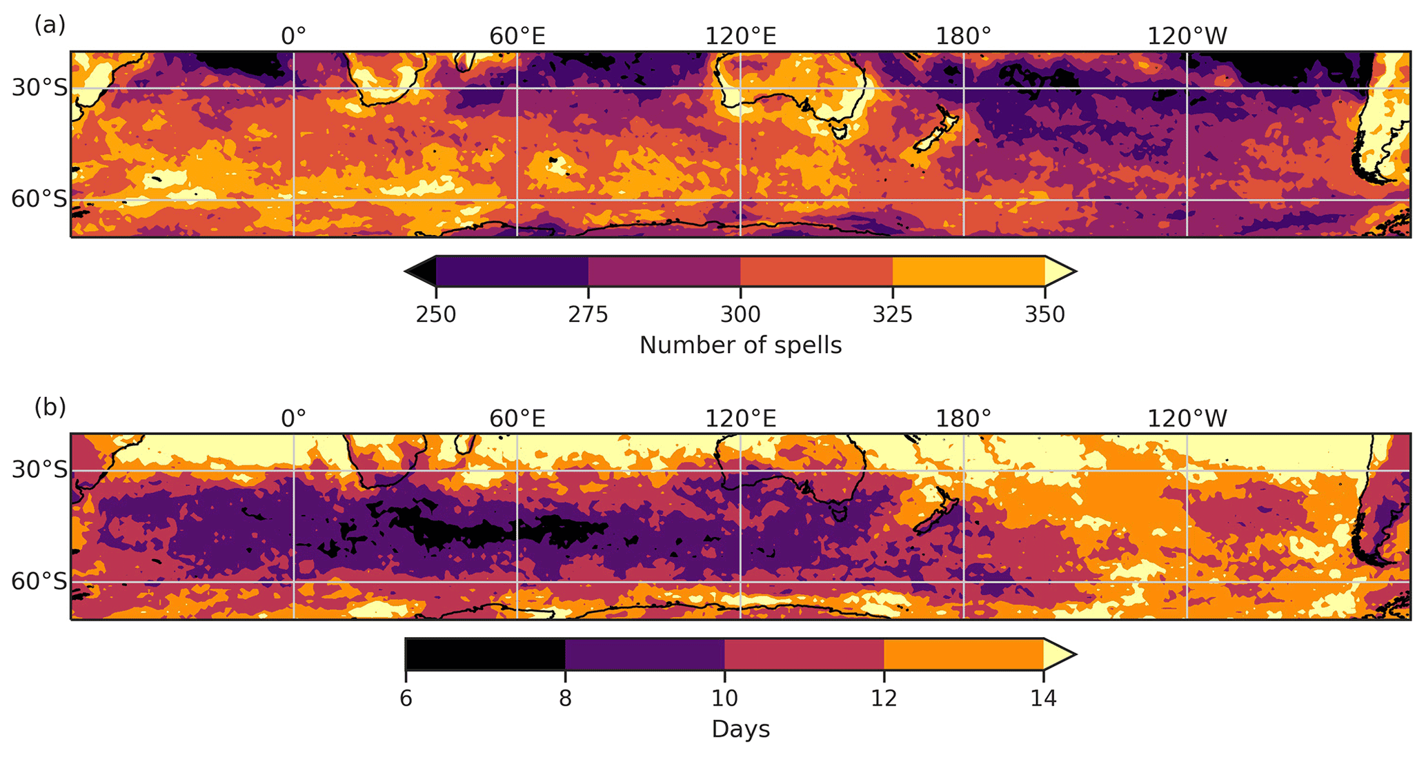
Figure 2 (a) Total number of hot spells in November–April identified at each grid point between 20 and 70^∘ S. (b) The 95th percentile of hot-spell durations in days.

2.6 Weibull regression model to assess the effect of RRWPs in the SH hot spells

To quantify the effect of RRWPs on the persistence of hot surface weather, we extend an analysis from Röthlisberger et al. (2019) to the SH, including SEA, using the same statistical model setup, a Weibull regression model. This model allows us to model the distribution of the duration of hot spells at each grid point. An advantage of the model of Röthlisberger et al. (2019) is that we do not need to subjectively define the duration of a “significant” spell because the model quantifies the changes in all quantiles of the spell duration modelled. The null hypothesis tested here at each grid point is that RRWPs have no effect on the duration of hot spells at the respective grid point. The Weibull model is only briefly introduced here. Please refer to Röthlisberger et al. (2019) for further details and their Supplement for a detailed introduction to the Weibull model.

To fit the Weibull model to the observed spell duration distribution, a representative value of the R metric needs to be assigned to each hot spell. This is achieved in the following way: for each hot spell i at grid point g with a duration D_g,i, the raw R metric R(λ,t) is longitudinally averaged within a 60^∘ longitudinal sector centred at the grid point g with longitude λ_g to yield R_lon(λ,t). Then, a median of R_lon(λ,t) is calculated for the lifetime of the hot spell to assign a representative value of R as ${\stackrel{\mathrm{̃}}{R}}_{{\mathit{\lambda }}_g,i}$ for each spell. The model is formulated as

$$\begin{array}{}\text{(2)}& \begin{array}{rl}\ln \left(D_{g,i}\right)=& {\mathit{\alpha }}_{\mathrm{0},g}+{\mathit{\alpha }}_{\mathrm{1},g}{\stackrel{\mathrm{̃}}{R}}_{{\mathit{\lambda }}_g,i}+\sum _{j=\mathrm{2}}^{\mathrm{6}}{\mathit{\alpha }}_{j,g}{m}_j\left(t_{g,i}^{\mathrm{start}}\right)\\ & +{\mathit{\sigma }}_g{\mathit{ϵ}}_{g,i};i=\mathrm{1},\mathrm{\dots },n_g.\end{array}\end{array}$$

Here, α_0,g is the intercept, α_1,g is the regression coefficient for ${\stackrel{\mathrm{̃}}{R}}_{{\mathit{\lambda }}_g}$, and ${\mathit{\alpha }}_{j,g},j=\mathrm{2},\mathrm{\dots },\mathrm{6}$ are regression coefficients for dummy variables $m_j\left(t_{g,i}^{\mathrm{start}}\right)$ that take the value 1 if spell i starts in month m_j and are zero otherwise. The coefficients α_j,g, therefore, account for possible seasonality in the spell duration distribution at grid point g (e.g. longer hot spells in May compared to e.g. September), while σ_g is a scale parameter and the ϵ_g,i are error terms. Exponentiated regression coefficients, e.g. exp (α₁), are usually referred to as the acceleration factor (AF). The exp (α₁) is of particular interest here, as it quantifies the factor of change in all quantiles of the distribution of spell duration distribution at grid point g per unit increase in $\stackrel{\mathrm{̃}}{R}$ (Hosmer et al., 2008; Zhang, 2016; Röthlisberger et al., 2019). An AF >1 implies an increase in all spell duration quantiles with increasing $\stackrel{\mathrm{̃}}{R}$ (i.e. during RRWPs) and conversely for an AF <1.

Furthermore, fitting Eq. (2) to spell durations at all grid points results in a spatial field of the AF. The statistical significance of the AF values is evaluated in a two-step approach. First, a p value for the above null hypothesis is computed exactly as in Zhang (2016). Then, the false-discovery-rate (FDR) test of Benjamini and Hochberg (1995) is applied to the resulting field of p values. The FDR test controls for type I errors, i.e. falsely rejecting the null hypothesis that can occur substantially in analyses like this one where multiple tests are being performed independently from each other at each grid point (e.g. Wilks, 2016). Here we follow the recommendation of Wilks (2016) and allow for a maximum false discovery rate α_FDR of 0.1.

3 Results

3.1 RRWPs and hot-spell durations

The Weibull analysis reveals that RRWPs are significantly correlated with the duration of hot spells in several regions within the SH and including over SEA (Fig. 3). Recall that an AF larger than 1 means that an increase in R is related to an increase in hot-spell duration and conversely for an AF smaller than 1. Thus, several parts of central and southern Australia, including the states of SA, VIC, NSW, and TAS, experience longer hot spells during periods when RRWPs occur. Northern Australia, however, does not show such a correlation with RRWPs, which agrees with previous studies showing different dynamical pathways for northern and southern Australian heatwaves (Risbey et al., 2018; Quinting and Reeder, 2017; Parker et al., 2020). Other statistically significant areas over land include parts of South America: southern Brazil, Bolivia, and parts of Argentina and Chile. For the Northern Hemisphere summer half-year, the significant AFs, larger than 1, form a wavenumber 7 pattern (Röthlisberger et al., 2019). In contrast, no clear wave pattern emerges for the SH in the significant AFs in Fig. 3. The difference in AF patterns between the two hemispheres is consistent with different climatological stationary wave patterns. The spatial pattern in Fig. 3 highlights areas where the transient waves building up the RRWPs have a predominant phasing in summer. In summary, the regression analysis shows that RRWPs are significantly associated with the duration of hot spells in several SH regions over land, including SEA. However, the Weibull analysis does not provide any information about the processes and hence potential causal link between RRWPs and the most intense SEA heatwaves. Accordingly, we next focus on SEA heatwaves and elucidate the role of RRWPs and blocks for two selected cases studies of SEA heatwaves and investigate further co-occurrence of SEA heatwaves and days with high R.

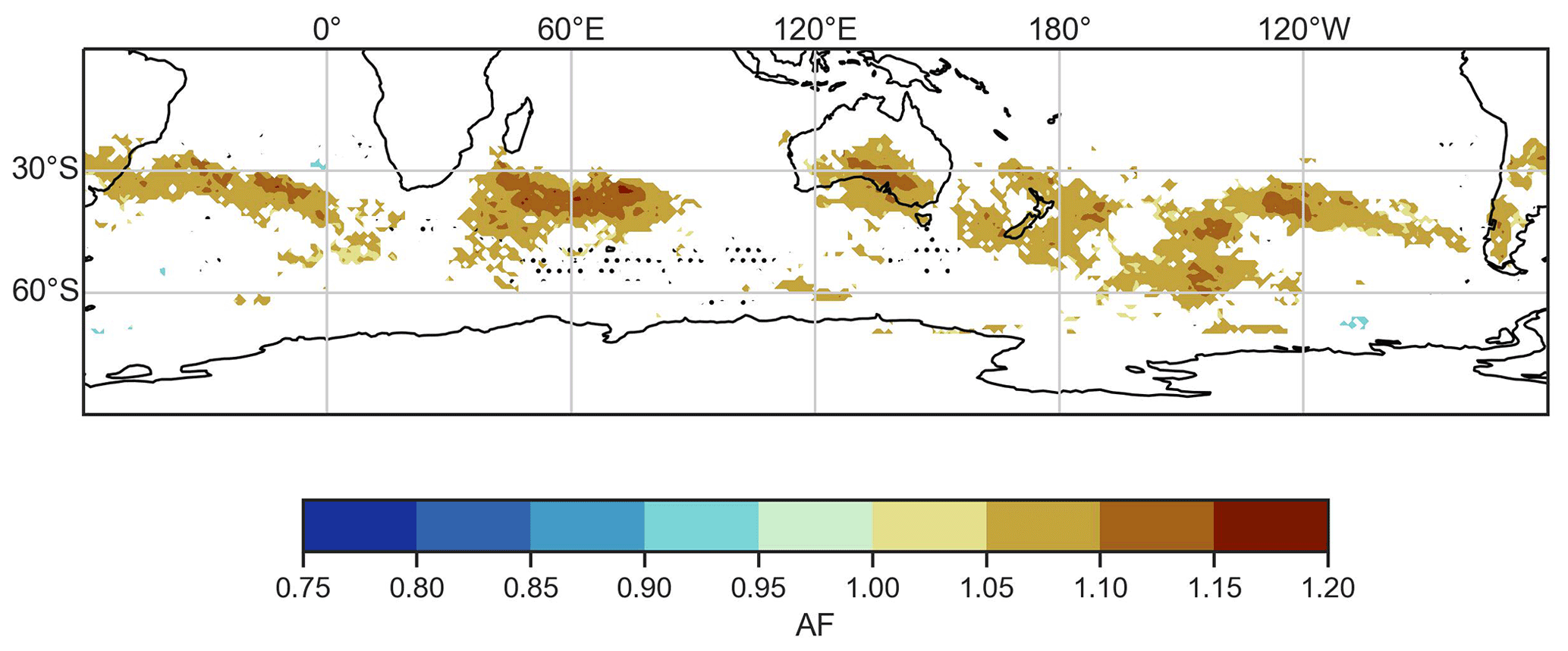
Figure 3 Statistically significant acceleration factors (AFs) for hot spells in November–April between 20 and 70^∘ S. Colours show AFs from a Weibull model with the R metric as a covariate. Stippling indicates grid points where spell durations do not follow the Weibull model based on the Anderson–Darling test at a significance level of 0.01.

3.2 RRWPs and blocks during two extreme and persistent SEA heatwaves

3.2.1 Case 1: 2004 heatwave

The February 2004 heatwave (7–22 February) lasted for 16 d. More than 60 % of continental Australia recorded temperatures above 39 ^∘C during this event (National Climate Centre, 2004). At the time, this event was the most severe February heatwave on record in both spatial and temporal extent and ranked in the top five Australian heatwaves for any month (National Climate Centre, 2004). More than 100 stations in SA, NSW, and northern VIC experienced record temperatures for February, and in some regions all-time records were set for consecutive days of heat (Bureau of Meteorology, 2004). Previous studies have shown that the upper-level anticyclonic PV anomalies over SEA during the heatwaves are associated with subsidence and is the major process causing the anomalies of high surface temperature (e.g. Quinting and Reeder, 2017; Parker et al., 2020). The surface flow associated with anticyclonic anomalies may also advect warm continental air due to the north-westerly flow at lower levels (e.g. Parker et al., 2014b). The warm advection associated with the surface flow can be significant even with weak upper- or lower-level winds. Here, we show how RRWPs contribute to persistent anticyclonic PV anomalies over SEA.

Figure 4 shows the flow conditions prior to and during the heatwave (Fig. 4b) and the corresponding T2m anomalies over SEA (Fig. 4a). The Hovmöller diagram (Fig. 4b) shows the 35 and 65^∘ S averaged meridional wind. Figure 5 shows the upper-level flow at different time steps prior to and during the heatwave. We use the two figures (Figs. 4 and 5) to demonstrate the role of transient RWPs and blocks during the heatwave and present that next.

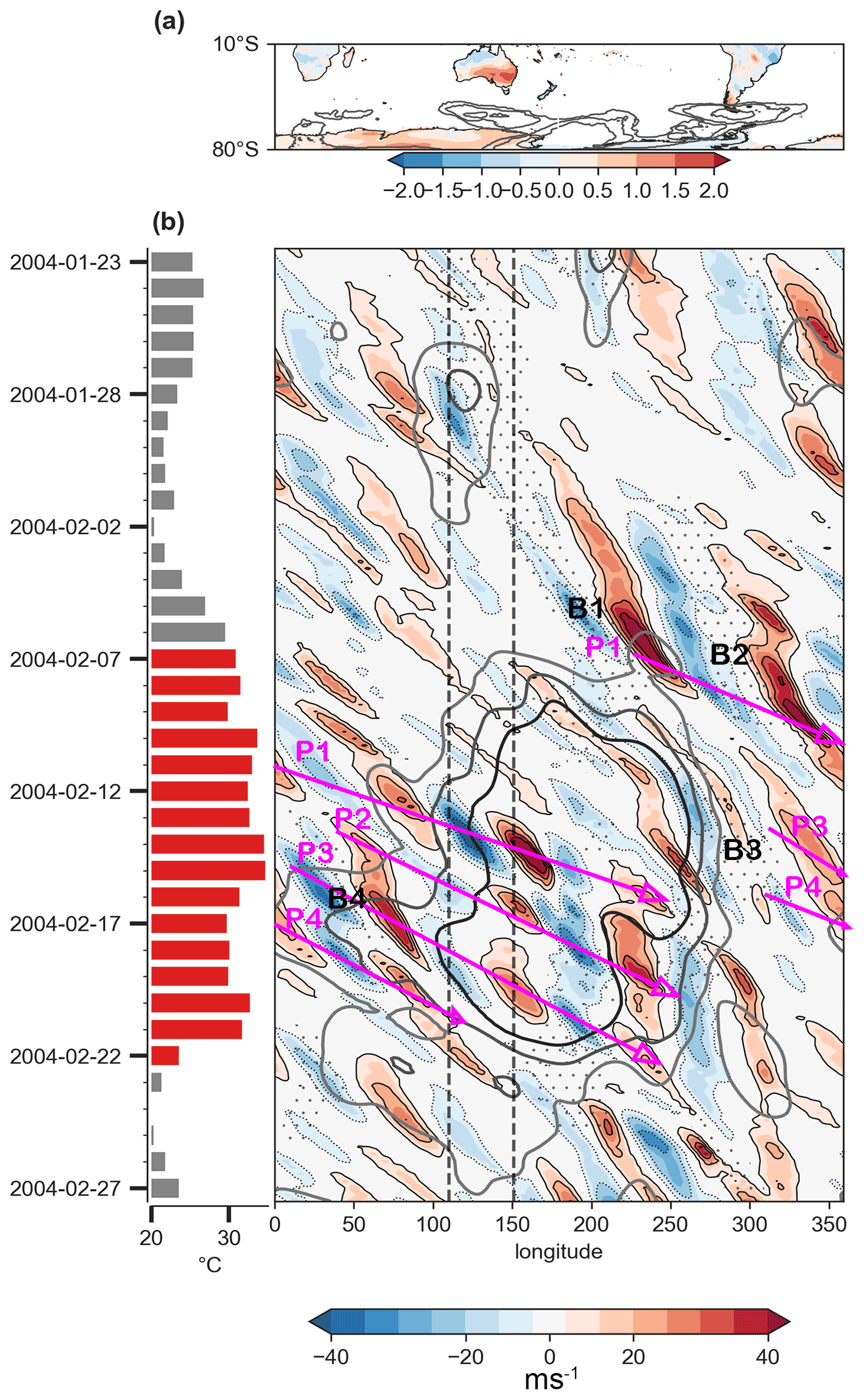
Figure 4 RRWPs and blocks during the 2004 SEA heatwave. (a) Filled contours depict the time mean of the standardized day-of-year anomalies of daily-maximum T2m over land for the duration of the heatwave. Contours show the mean blocking frequency during the heatwave (5 %, 10 %, 20 %). (b) Bars show daily-maximum 2 m temperature averaged over SEA (^∘C); red marks the heatwave period. The Hovmöller diagram shows the meridional wind at 250 hPa averaged between 35 and 65^∘ S (filled contours; m s⁻¹), R values (grey contours; 6, 8, 10 m s⁻¹), and longitudes at which at least one grid point between 40 and 70^∘ S featured an atmospheric block (stippling). Rossby wave packets (blocks) are labelled in magenta (black).

Figure 5 (a–f) Meridional velocity at 250 hPa (colour shading), 2 PVU contours at isentropes 340 K (grey line) and 350 K (black line) at various time steps. Stippling and orange contours show blocks identified using a 1.3 and 1.0 PVU threshold, respectively.

During this event, several Rossby wave packets were observed, recurrently amplifying in the same phase, forming a ridge over SEA. The upper-level flow over SEA was zonal prior to the heatwave (Fig. 5a). An upper-level ridge forms over SEA around 5 February prior to the heatwave (Fig. 5b). The flow becomes more amplified in the subsequent days with a circumglobal amplified wave pattern apparent around 9 February (Fig. 5c). The amplified wave, part of a transient and nonstationary Rossby wave packet (RWP; P1 in Fig. 4b) arrived over the southern Indian Ocean, and an upper-level ridge began to form over Australia, which amplified further around 13 February (Fig. 5d). Two further ridges formed over SEA on 16 and 18 February (Fig. 5e, f), each ridge being part of a transient nonstationary RWP initiated upstream of Australia (P3, P4 in Fig. 4b). These series of upper-level recurrent ridges were part of the RRWPs and contributed to the persistence of the heatwave. These recurrent ridges associated with RRWPs were also detected by the R metric (grey contours in Fig. 4b).

No blocks were identified directly over SEA during the heatwave, but blocks were present south of SEA and further downstream (Figs. 4, 5). The RWP labelled as P1 in Fig. 4b formed downstream of block B1 in the Pacific Ocean (roughly 200^∘ E, i.e. 160^∘ W), where the block moved from south of Australia a few days earlier (Fig. 5a). Block B2 was simultaneously present in the vicinity of South America around 7 February (Fig. 4b). In the next few days, simultaneous wave breaking was observed in the central Pacific Ocean and south of Africa in the Indian Ocean. Another set of RWPs (P3 and P4 in Fig. 4b) were associated with a block over the Pacific Ocean (B3 in Figs. 4b, 5d). Simultaneously, another block was present south of South Africa (B4 in Figs. 4b, 5d). Block B4 was also associated with amplified Rossby waves downstream over the Indian Ocean on 16 February (Fig. 5e). Thus, we argue that blocks could have played a key role in the initiating, phasing, and meridional amplification of the four Rossby wave packets (P1–P4) that reached Australia between 13 and 18 February. In summary, we saw recurring RWPs that passed over Australia during this period (Fig. 4b). These waves were not stationary; they were not triggered in the same area or over Australia; and they were initially not in phase upstream of Australia.

3.2.2 Case 2: 2009 heatwave

The 2009 heatwave (27 January–9 February), although extensively covered in literature (e.g. Engel et al., 2013; Parker et al., 2014b), has been chosen because it is one of the most severe heatwaves in SEA. It lasted for 14 d. Between 28–31 January and 6–8 February, temperatures in SEA were exceptionally high. On Black Saturday, 7 February, the hot, dry, and windy conditions fuelled many catastrophic fires in VIC, which recorded 173 fatalities, and more than 2133 houses were destroyed (Karoly, 2009; Parker et al., 2014b; VBRC, 2010). During this heatwave, an anticyclone over SEA and the associated north-westerly flow at the surface advected hot continental air into SEA leading to extreme surface temperatures (Parker et al., 2014b). As for the 2004 case, we next present the Hovmöller diagram (Fig. 6) and snapshots of upper-level flow (Fig. 7) to demonstrate the role of transient RWPs and blocks during the heatwaves.

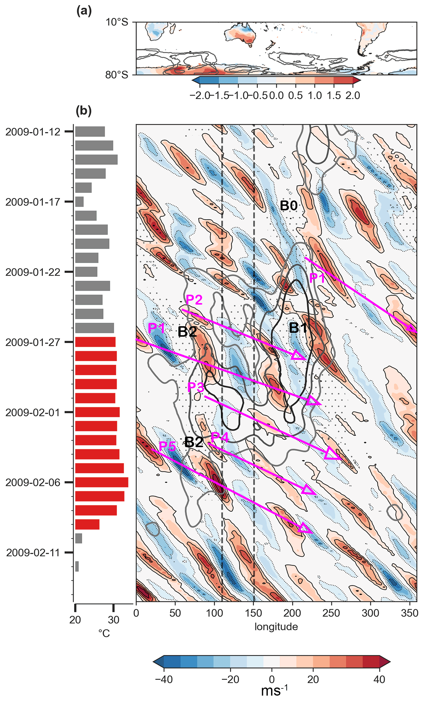
Figure 6 Same as in Fig. 4 but for the February 2009 SEA heatwave.

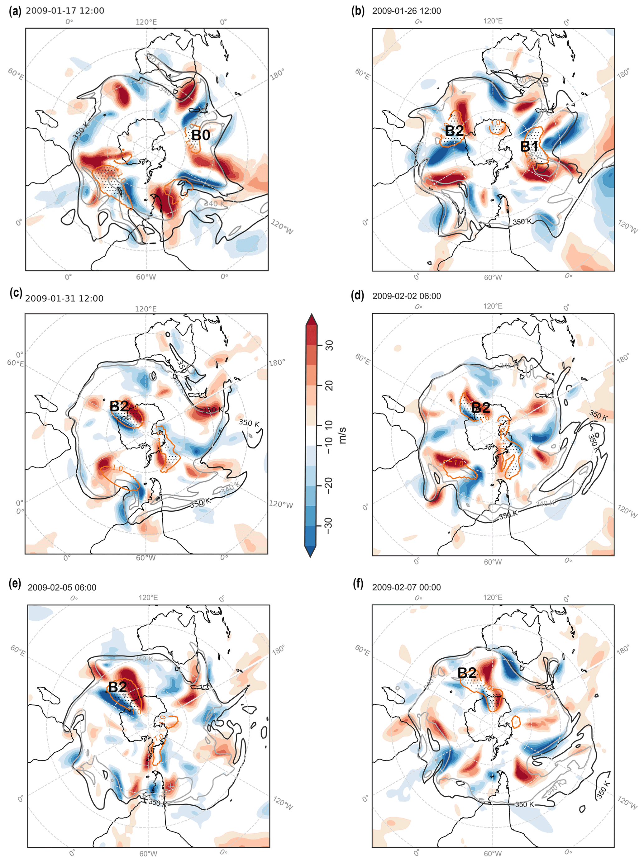
Figure 7 Same as in Fig. 5 except for the February 2009 SEA heatwave.

Prior to the onset of the heatwave, the flow was already amplified with a wave breaking over SEA (Fig. 7a). Several RWPs were observed prior to and during this event (P1 and P2 in Fig. 6b). The RWPs prior to the heatwave were not in the same phase as those during the heatwave (Fig. 6b), which is why the value of the R metric is not high around 25 January. Around 26 January, a Rossby wave packet (P2 in Fig. 6b) was observed forming an upper-level ridge over Australia (Figs. 6b, 7b). In the subsequent days, the amplified wave broke anticyclonically over SEA (Fig. 7c), resulting in an anticyclonic PV anomaly over SEA (see Parker et al., 2014b, for a detailed analysis of this event). On 2 February, a new ridge started forming over southern Australia (Fig. 7d) as part of a Rossby wave packet (P3 in Fig. 6b) and reached over SEA on 5 February (Fig. 7e). However, the upper-level ridge was transient and was replaced by another ridge around 7 February as part of another amplified wave (P4 in Figs. 6, 7f).

No blocks were identified directly over SEA during the heatwave (Figs. 6, 7). However, blocks were frequent upstream of SEA from 50 to 70^∘ E in the Indian Ocean (B2 in Figs. 6b, 7) and downstream of SEA from 200 to 250^∘ E (i.e. 160 to 110^∘ W; B1 in Figs. 6b, 7). Block B2 over the Indian Ocean was particularly persistent and interacted with several amplified Rossby wave packets (P2, P4). B2 began to weaken around 2 February (Fig. 7d) but restrengthened again on 5 February (Fig. 7e) due to absorption of low PV from a smaller southward block in the Indian Ocean (not shown). Therefore, B2 remained persistent throughout the heatwave. Rossby wave packet P1 formed downstream of block B0 over the Pacific Ocean prior to the heatwave (Figs. 6b, 7a).

So far, we have investigated the association of RRWPs with a duration of hot spells. We also presented two cases of extreme and persistent SEA heatwaves to show how RRWPs can lead to the formation or replenish the anticyclonic PV anomalies over SEA. Figure B1 shows another case of SEA heatwave associated with RRWPs. In the next section, we extend the analysis to a climatological period (1979–2018) and explore high-R_SEA conditions for all the SEA heatwaves.

3.3 RRWP conditions during SEA heatwaves

First, we note the co-occurrence of high-R_SEA days and SEA heatwave days (SEA HDs) as defined in Sect. 2.3. Out of 352 d with high R_SEA, 67 co-occur with SEA HDs, and 285 do not co-occur (Table C1). Thus, the conditional probability of a SEA HD given high R_SEA is 0.19 $(\mathrm{67}/\mathrm{352}=\mathrm{0.19})$, which is higher than the climatology $(\mathrm{457}/\mathrm{3520}=\mathrm{0.13})$. The conditional probability further increases to 0.34 on filtering out the high-R_SEA days containing a cyclonic PV anomaly over SEA (Table C1). Many high-R_SEA days do not co-occur with SEA HDs, which indicates that R is not a sufficient condition for SEA heatwaves on its own. We, therefore, further explore why some high-R_SEA days co-occur with SEA HDs, while others do not.

High-R_SEA days co-occurring with SEA HDs feature a large anticyclonic PV anomaly over SEA (Fig. 8a) on the 350 K isentropic surface. The 2 PVU isoline on the 350 K isentropic surface, indicating the dynamic tropopause, is also located over SEA, thereby indicating a suitable choice of the isentropic surface. Areas upstream and downstream of the anticyclonic PV anomaly over SEA feature cyclonic PV anomalies that are also located equatorward of the highest blocking frequencies (black contours in Fig. 8a). These may correspond to the cyclonic PV anomalies surrounding omega-type blocking or the cyclonic PV anomalies of the dipole blocks. Since blocking is a binary dataset, the blocking frequency in Fig. 8 indicates the percentage of days on which a grid point features a block. Thus, for high-R_SEA days co-occurring with SEA HDs, blocks are more frequent over the Indian and the South Pacific oceans close to the Antarctic coast (Fig. 8a) compared to high-R_SEA days without co-occurring SEA HDs (Fig. 8b, c) and are less frequent over the 60^∘ S latitude, the latitudinal band featuring a high blocking frequency in the DJF climatology (Fig. 8c, f).

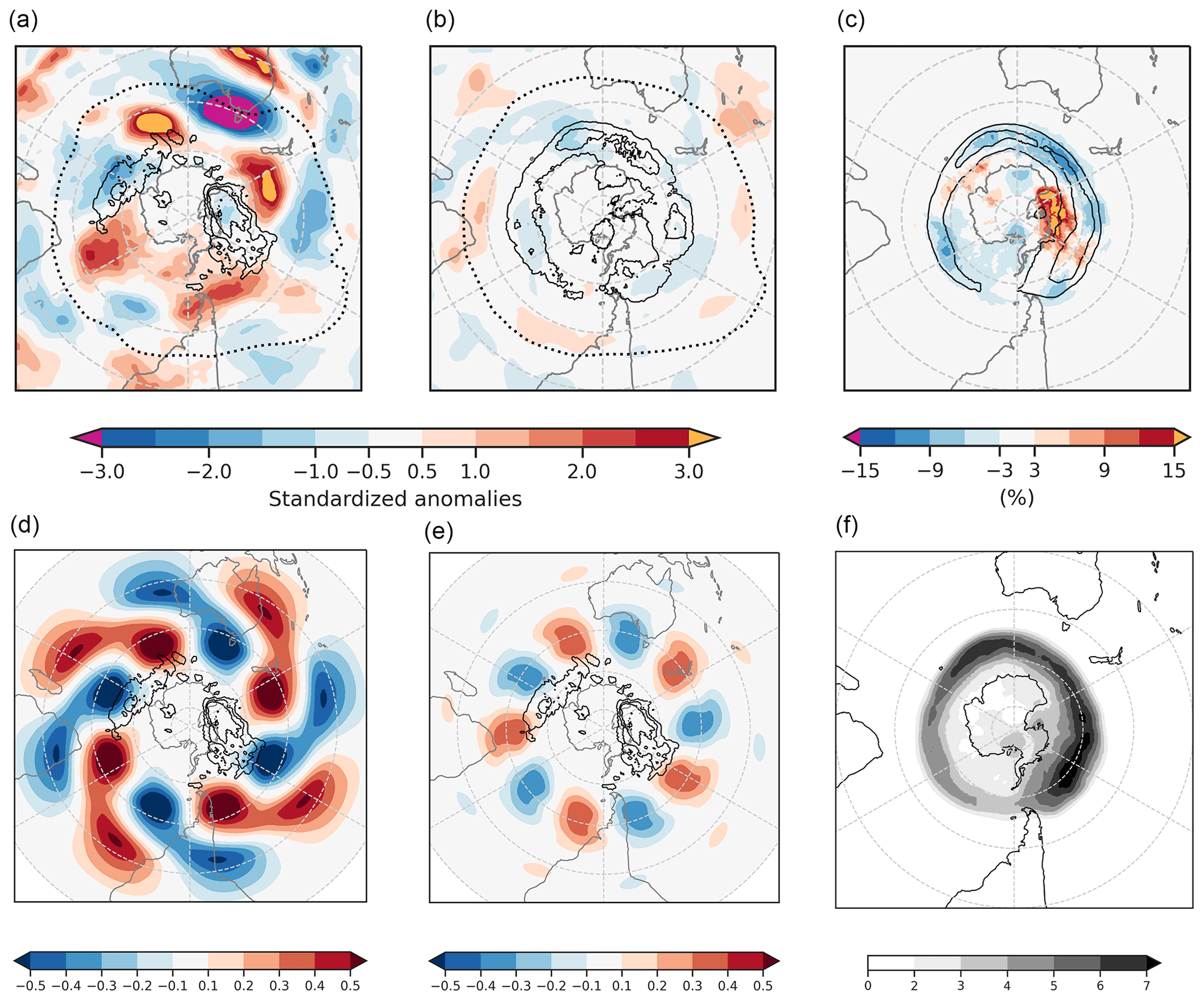
Figure 8 Standardized PV anomalies on the 350 K isentrope with respect to the DJF climatology (1979–2018) for (a) high-R_SEA days and SEA heatwave days (HDs) and (b) high-R_SEA days and non-SEA HDs. Dotted black lines show a 2 PVU contour in the mean PV fields for panels (a) and (b), and black contours show mean blocking frequency contours at 5 %, 10 %, and 15 % for the same. (c) The difference in blocking frequency between panels (a) and (b). (d) The WN4 and (e) WN5 component for the mean PV (in PVU) for high R_SEA and SEA HDs in panel (a), with black contours showing the blocking frequency as in panel (a). (f) The climatological mean blocking frequency (%) for DJF; black contours in panel (c) show the same at 4 % and 6 %.

In contrast, on high-R_SEA days not co-occurring with SEA HDs (Fig. 8b), there is no clear anticyclonic PV anomaly over SEA. Weak zonally elongated PV anomalies are present over the ocean basins, which are co-located with the blocking frequency fields south of South Africa and in the Indian and South Pacific oceans (black contours in Fig. 8b). The difference in the spatial distribution of PV anomalies on the high-R_SEA days not co-occurring with SEA HDs and the high-R_SEA days co-occurring with SEA HDs suggests that only the RRWPs whose phase is conducive to forming ridges over SEA are important for SEA heatwaves. Furthermore, Fig. D1 shows the PV composite for all SEA HDs.

In addition to the ridge over SEA, circum-hemispheric zonal wavenumber 4 and 5 (WN4, WN5) patterns are present in the composite mean PV fields for high-R_SEA days co-occurring on SEA HDs (Fig. 8a), where five distinct highs (negative PV anomalies) and four lows are visible in the 30 to 60^∘ latitudinal band. We hypothesize that Rossby waves in a particular phase help to establish the anticyclonic PV anomalies over SEA (in Fig. 8a). Hence, we present Fourier decomposition of the composite mean PV field for high-R_SEA days co-occurring with SEA HDs (Fig. 8d, e). To check for a preferred phasing during high-R and SEA HDs, we also present the phase–amplitude distribution of the meridionally averaged meridional wind v_ma later in Fig. 9.

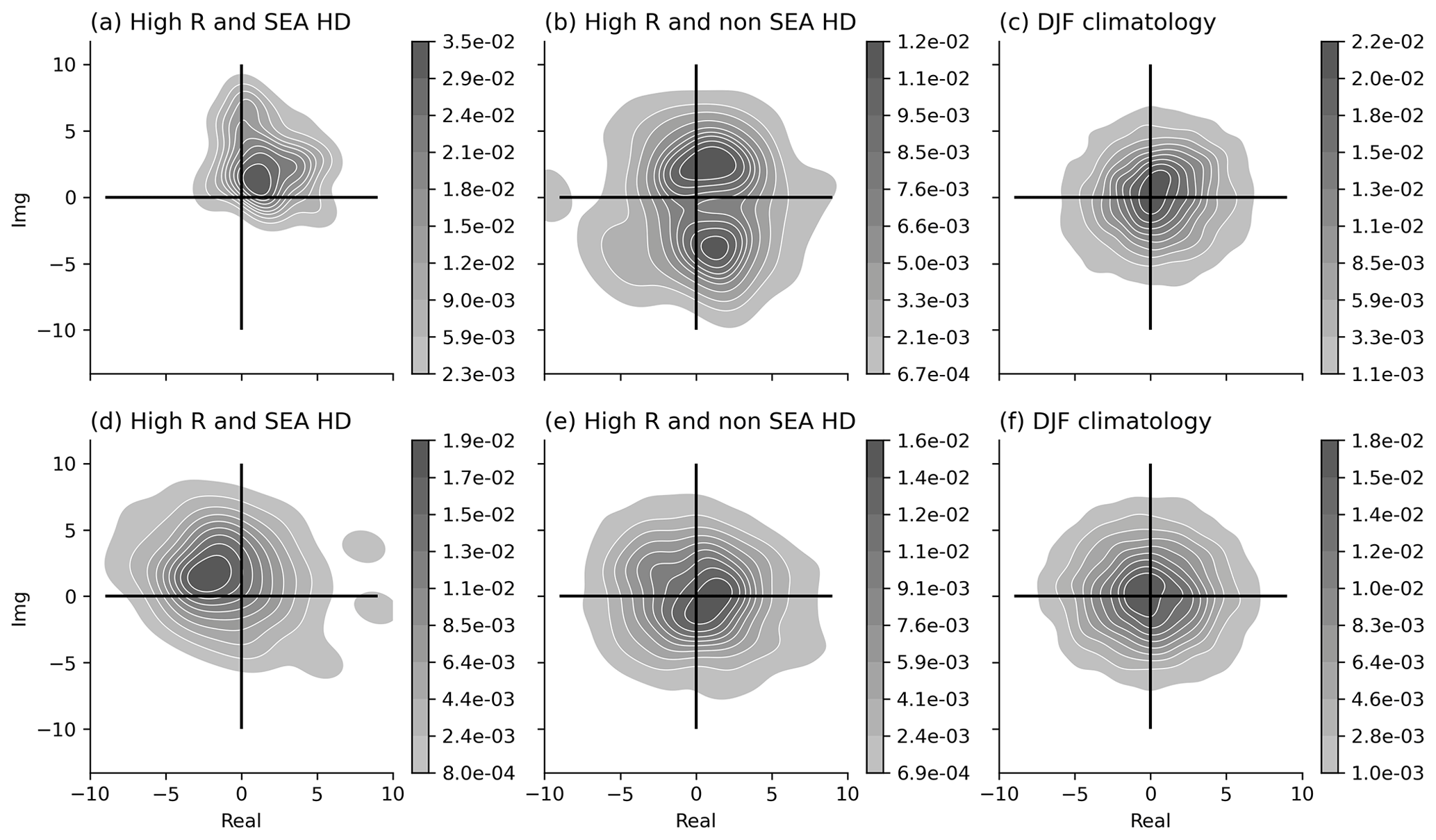
Figure 9 Bivariate kernel density estimate using Gaussian kernels in the complex plane of the Fourier decomposed meridional wind at 250 hPa averaged between 35 and 65^∘ S. Only zonal WN4 (a, b, c) and WN5 (d, e, f) are shown for days belonging to (a, d) high R_SEA and SEA HDs, (b, e) high R_SEA and non-SEA HDs, and (c, f) DJF climatology.

The WN4 and WN5 components (Fig. 8d, e) of the composite mean PV field for high-R_SEA days co-occurring with SEA HDs bring out the role of the phase of the waves in contributing to the anticyclonic anomalies over SEA in Fig. 8a more clearly. Over SEA, both WN4 and WN5 components have the same phase and contribute to the anticyclonic PV anomalies. The north-east and south-west orientation in the WN4 pattern over Australia may be associated with the anticyclonic wave breaking over Australia. In the South Pacific and Indian oceans, we observe cyclonic PV upstream and downstream of the blocking frequency contours (Fig. 8d, e).

Figure 8d and e suggest that high-R_SEA days that co-occur with SEA HDs have a particular phase conducive to forming anticyclonic PV anomalies over SEA. Therefore, as stated earlier, we next present the phase–amplitude distribution for WN4 and WN5 components to test this hypothesis in Fig. 9 for the latitudinally averaged (35–65^∘ S) daily meridional wind velocity at 250 hPa as v_ma. We compare the density distribution for days with high R_SEA and SEA HDs with high R_SEA and non-SEA HDs. Using a Fourier decomposition (see Sect. 2), we extract the WN4 and WN5 components and plot the phase and amplitude density distribution on a complex plane using a Gaussian kernel density estimate (KDE). To determine the amount of smoothening, we used the default bandwidth estimation method, the Scott method. Since we are interested in the qualitative spread of the WN components (e.g. unimodal, bimodal) rather than quantitative estimation of the probability density function, the choice of our smoothening parameters for the KDE is sufficient.

On high R_SEA and SEA HDs, the density distribution of the WN4 component in the complex plane is unimodal (Fig. 9a), which points to a preferred phase of the waves. From Fig. 8d, we know that it predominantly forms an anticyclonic PV anomaly over SEA. The density distribution of WN4 for high R_SEA and non-SEA HDs has a broader bimodal spread. The distance from the origin of the complex plane represents the amplitude; hence, the peak of the WN4 distribution of high-R_SEA days has a higher amplitude (Fig. 9a, b) compared to the DJF climatology whose peak is almost centred at the origin (Fig. 9c). For WN5, the peak of the distribution for days with high R_SEA and SEA HDs have a different phase and higher amplitude compared to high R_SEA and non-SEA HDs (Fig. 9c, d) and the DJF climatology (Fig. 9e).

The phase distribution for WN4 and WN5 is shown here because they emerge as the dominant patterns in the composite mean (Fig. 8a), whereas the density distributions for other wavenumbers (k=3, 6, 7) do not exhibit a clear difference between high R_SEA and SEA HDs compared to high R_SEA and non-SEA HDs and DJF climatology (not shown). Overall, our results agree with the understanding of SEA heatwaves featuring upper-level anticyclonic PV anomalies over SEA (Marshall et al., 2014; Parker et al., 2014b; Quinting and Reeder, 2017), and we show how RRWPs in a particular phase (WN4 and WN5) are conducive to forming anticyclones over SEA.

4 Discussion

During the 2004 and 2009 SEA heatwaves, we find transient and fast-moving Rossby waves organized in wave packets recurring in the same phase to form a ridge over SEA, thereby contributing to the persistence of the heatwave conditions. This persistence arises by recurrence, in contrast to the persistence arising from stationary weather features such as slow-moving Rossby waves (e.g. Wolf et al., 2018) or blocking anticyclones (e.g. Kautz et al., 2022). The Rossby wave packets observed during the two SEA heatwaves were not always initiated in the same area. In the 2004 case, these waves were mostly not in phase upstream of Australia, whereas in the 2009 case, they were also in phase upstream over the Indian Ocean. Blocks were observed upstream and downstream during the two heatwaves, which suggests that blocks could play a role in initiating the RWPs and/or in modulating their phase. Figure E1 presents the relationship between R anomalies and the blocks in the Indian and South Pacific oceans for DJF. Overall, our results agree with Risbey et al. (2018) and King and Reeder (2021), who reported transient waves in the Indian Ocean preceding SEA heatwaves and transient circulation anomalies during SEA heatwaves. More specifically, we show how recurrent Rossby waves aid in the persistence of the well-known upper-level anticyclonic PV anomalies during SEA heatwaves by forming recurrent upper-level ridges.

The relevance of RRWPs for persistent SEA heatwaves documented in these two case studies is consistent with the results of the Weibull regression analysis, which reveals a significant positive statistical link between the duration of hot spells over SEA and RRWPs. The PV composite for high-R_SEA days co-occurring with SEA heatwaves shows an anticyclonic PV anomaly over SEA (Fig. 8), which is a typical feature of SEA heatwaves (Parker et al., 2014b; Quinting and Reeder, 2017). The PV composite also shows wavenumber 4 and 5 (WN4, WN5) patterns, where the anticyclonic PV anomalies are located upstream and downstream of blocking frequency maxima. Furthermore, the WN4 and WN5 components of the mean PV field (Fig. 8d, e) as well as the phase–amplitude distribution of the WN4 and WN5 components of the meridional wind velocity (Fig. 9a, d) indicate a preferred phasing for high-R_SEA days part of SEA heatwaves. The results from the Weibull regression analysis also suggests preferred phasing of the transient eddies not only over SEA but also upstream and downstream of it. Therefore, recurrent Rossby wave packets in the right phase could help to foster the anticyclonic anomalies over SEA for time periods exceeding the lifespan of an individual wave packet. Hence, the combined evidence from the literature summarized above, together with the observations from the two case studies and the results from the regression analysis, suggests a causal link between RRWPs and persistent SEA heatwaves. The proposed link works as follows: heatwaves over SEA are forced by subsidence occurring in anticyclones of SEA (e.g. Quinting and Reeder, 2017). RRWPs result in the repeated formation of these ridges over SEA and thereby contribute to the persistence of the ridges and thus, the heatwaves. However, not all SEA HDs are associated with RRWPs, and hence other dynamical pathways for SEA heatwaves exist. In addition, local negative soil moisture anomalies strengthen positive temperature anomalies through increased surface sensible heat fluxes and may thereby extend the duration of heatwaves (e.g. Green, 1977; Seneviratne et al., 2010; Martius et al., 2021).

A reverse causal link between surface temperature anomalies during SEA heatwaves and R_SEA is theoretically possible, namely that the positive surface temperature anomaly contributes substantially to the upper-level ridge and that this ridge amplification increases R_SEA. This causal link cannot be distinguished in our Weibull model setup. However, model experiments from Martius et al. (2021) suggest that the influence of surface temperature anomalies over Australia on the upper-level (250 hPa) geopotential height and wind anomalies is quite small; therefore, the imprint on the R metric after the latitudinal averaging is even smaller.

5 Conclusions

We find that RRWPs are associated with a significant increase in the persistence of hot spells in the SH. In several parts of SEA, including the states of South Australia, New South Wales, Victoria, and Tasmania, longer hot spells coincide with high-amplitude RRWPs (Fig. 3). Other regions over land where RRWPs are statistically associated with hot-spell duration include South America: southern Brazil, Bolivia, and parts of Argentina and Chile.

We have demonstrated the role of RRWPs in building persistent ridges during two cases of SEA heatwaves: the 2004 and 2009 heatwaves. Both heatwaves featured RRWPs comprised of transient Rossby waves, which were in phase regionally but not hemisphere wide. Blocks were not directly observed over SEA, but the case studies suggest that blocks upstream and downstream played an important role in initiating the Rossby wave packets and modulating their phase. We further investigated the co-occurrence of RRWPs during the most persistent and extreme SEA heatwaves using the R metric.

We find that days with R exceeding the 90th percentile, high-R_SEA days, are associated with increased probabilities of being part of a heatwave (0.19) compared to climatology (0.13). These conditional probabilities have similar magnitudes as those with remote drivers, e.g. Madden–Julian oscillation (MJO) and El Niño–Southern Oscillation (ENSO) (Parker et al., 2014a). However, not all high-R_SEA days are associated with heatwaves. Further investigations suggest that those high-R_SEA days, which are relevant for the SEA heatwaves, play a role in forming or sustaining the ridges over SEA. Such high-R_SEA days exhibit circumglobal zonal wavenumber 4 and 5 (WN4, WN5) patterns in the PV composite and indicate a preferred phasing of the waves which is different from the DJF climatology. The high-R_SEA days that do not coincide with SEA heatwave days have a bimodal phase distribution in the WN4 component and result in a cyclonic PV anomaly over SEA. Therefore, R accompanied with information on the phasing of the wave packets could be used as a diagnostic metric for SEA heatwaves. Upon filtering out days forming a cyclonic PV anomaly over SEA, the conditional probability of SEA heatwave day given high-R_SEA days increased to 0.34.

The following open questions remain: what is the role of blocks in initiating RRWPs and modulating their phase? The case studies and the PV composites suggest that blocking might play an important role. What is the role of background flow in setting up RRWPs and modulating their phase? The interaction of RRWPs with other well-known climate oscillation patterns such as the ENSO and the Southern Annular Mode also needs to be investigated further. Better understanding of the interplay between these features might offer an opportunity to improve sub-seasonal forecasts during RRWP events.

Appendix A: Comparison of R anomalies for the Southern Hemisphere and Northern Hemisphere

R anomalies are calculated for each day of the year at each longitude from the mean of the day-of-year mean. Therefore, the R anomalies at each longitude show variation with the mean of the day-of-year mean and have a seasonal pattern. The magnitude of the anomalies shows that there is larger variation in the values for the NH than the SH. Both the Southern and Northern Hemisphere R fields show seasonality. Anomalies are highest for Northern Hemisphere boreal autumn and winter days. Interestingly, the Southern Hemisphere shows higher R anomalies during austral summer days than winter days.

Figure A1 R anomalies for the Southern and Northern Hemisphere. Anomalies for the day-of-year mean are calculated with respect to mean R fields.

Appendix B: RRWPs during the 2014 heatwaves

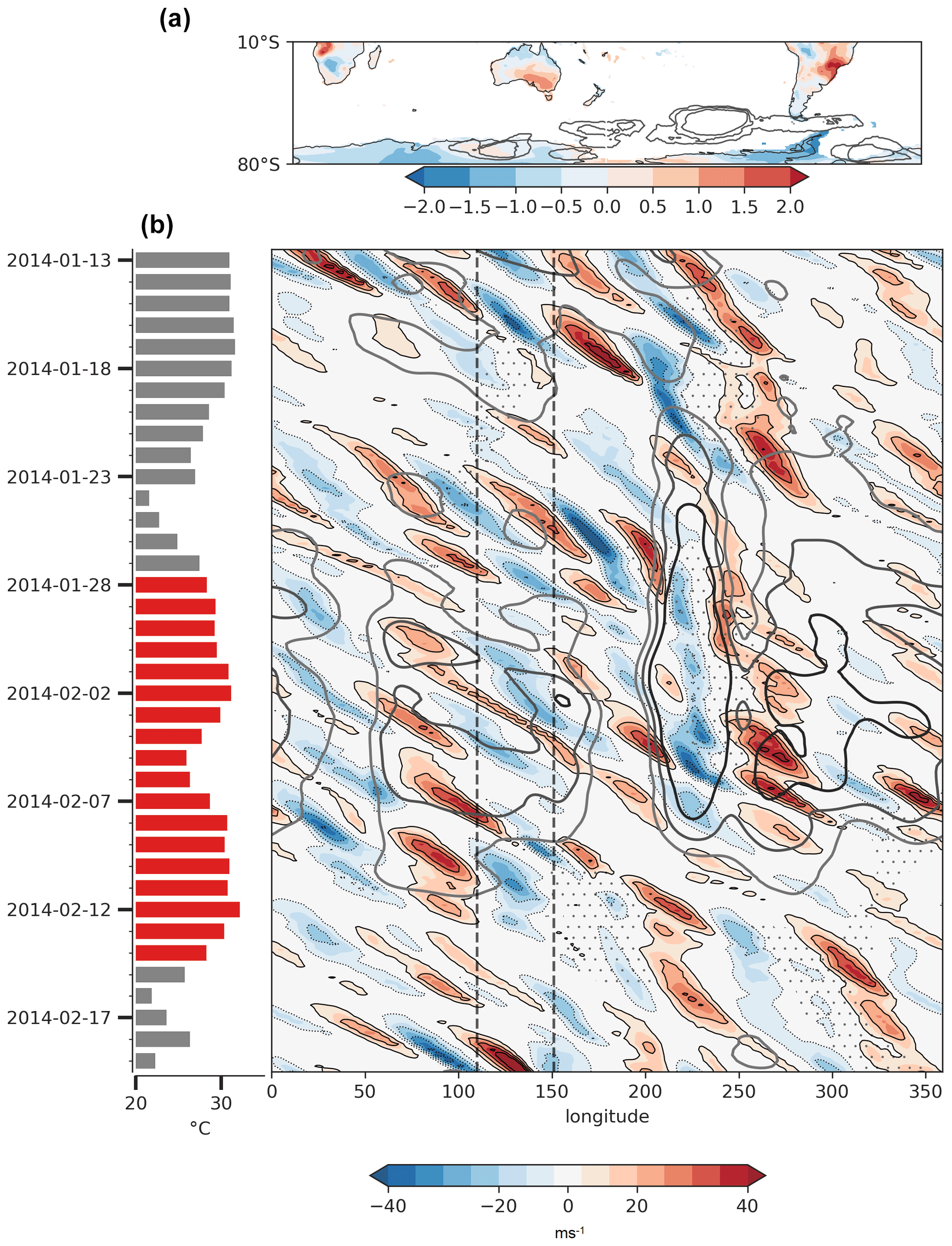
Figure B1 Same as in Fig. 4 but for January 2014 SEA heatwave.

Appendix C: Occurrence of high R_SEA on SEA heatwave days

Table C1 Occurrence of high R_SEA on SEA heatwave days and the associated conditional probabilities of a heatwave given high R_SEA, where high R_SEA (ridges) in the last column is calculated from taking the 90th percentile only from the days in DJF having an anticyclonic PV anomaly over SEA (30–45^∘ S, 130–153^∘ E).

Appendix D: PV composite for SEA heatwave days

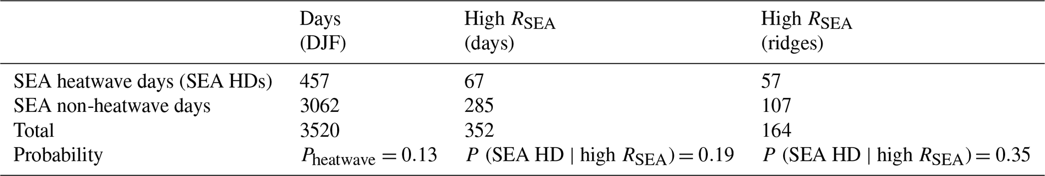
Figure D1 shows PV anomalies for all SEA heatwaves days identified in this study. The PV anomalies for SEA heatwaves feature anticyclonic PV anomalies over SEA with cyclonic PV anomalies to the north and south of it, which is similar to Fig. 2 in Parker et al. (2014b), who show PV anomalies for Victorian heatwaves. However, the wavenumber pattern seen in Fig. 8a for SEA HDs and high R_SEA is not clear for all SEA HDs in Fig. D1b.

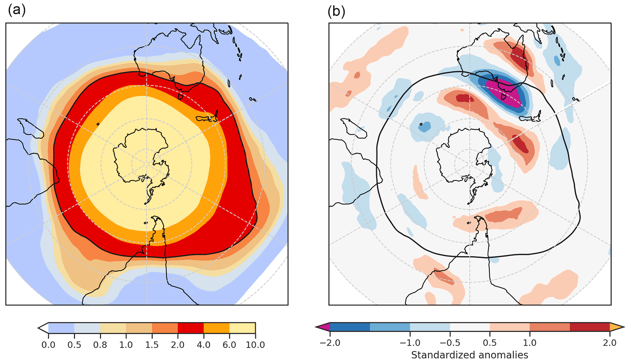
Figure D1 (a) PV composite mean at 350 K isentrope for SEA heatwave days and (b) the respective anomalies with DJF mean climatology.

Appendix E: Relationship between blocks and RRWPs in the South Pacific and Indian oceans

To further analyse the spatial distribution of RRWPs relative to blocks in the SH, we focus on two longitudinal subdomains that show a high blocking frequency in the DJF climatological mean: the South Pacific (130–50^∘ W) and Indian oceans (0–90^∘ E). We use time-lagged composite R anomalies with respect to the centroid of the blocks at the time of the maximum blocking amplitude in the two domains similar to Röthlisberger et al. (2019; see Fig. 12 in their paper). Here, R anomalies are calculated with respect to the day-of-year climatology.

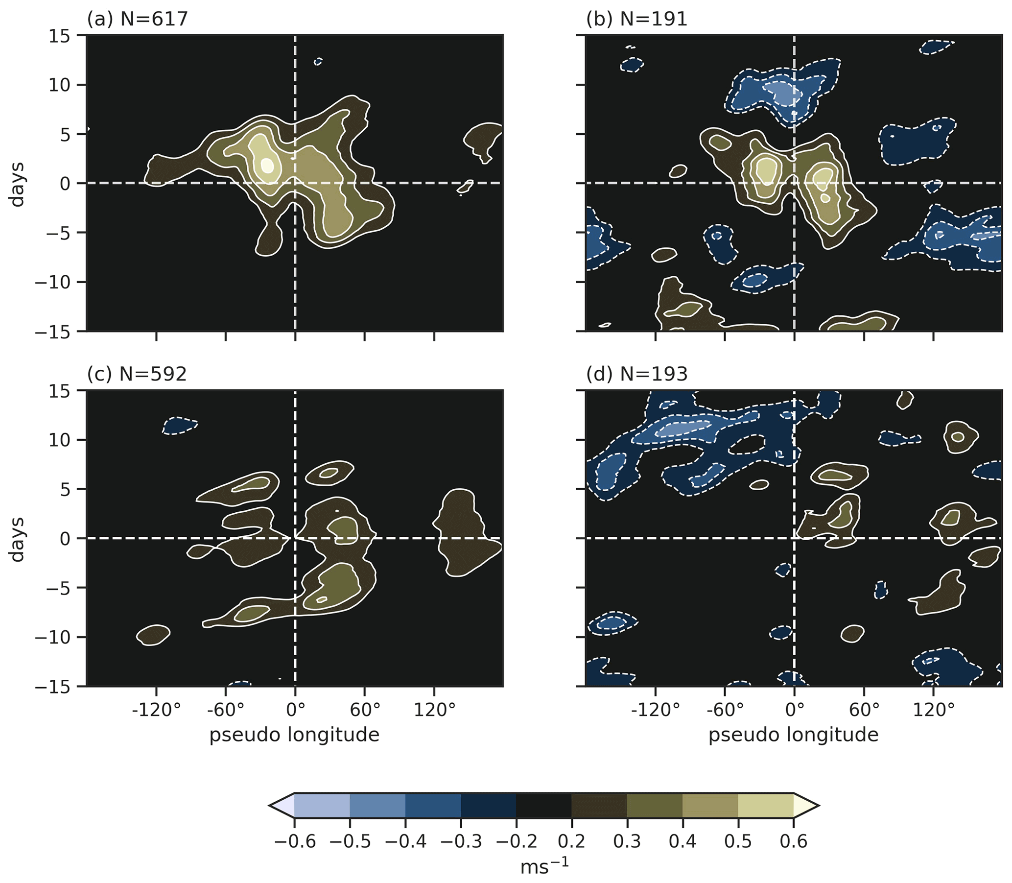
Figure E1 Time-lagged Hovmöller composites of R anomalies centred on the mean longitude and time of maximum amplitude of blocks located in the Pacific Ocean (180–60^∘ W, 30–80^∘ S) in panels (a) and (b) and Indian Ocean (60–180^∘ E, 30–80^∘ S) in panels (c) and (d). Left column includes blocks for all seasons, and right column shows them for DJF. N denotes the number of blocks for each category.

In the Pacific Ocean, blocks coincide with positive R anomalies in a longitudinal band from ∼60^∘ upstream to ∼60^∘ downstream of the blocks (Fig. E1a, b) from 5 to 8 d before the time of maximum blocking amplitude; this resembles a butterfly pattern, similar to blocks in the NH (Fig. 12 in Röthlisberger et al., 2019). Similar to the NH, R anomalies in the Pacific Ocean are not high at the centroid of the block. This could be because the wavelength of the upper-level ridge associated with the block may be too wide to be captured by the R metric because the R metric only has contributions from k=4 and higher. R anomalies are consistent for DJF and blocks for all seasons in the Pacific. In contrast, in the Indian Ocean, seasonal variation is seen in R anomalies (Fig. E1c, d), where DJF blocks show R anomalies downstream of the centroid of the block only and possibly shows weak association with RRWPs.