Identification of high-wind features within extratropical cyclones using a probabilistic random forest – Part 1: Method and case studies

Strong winds associated with extratropical cyclones are one of the most dangerous natural hazards in Europe. These high winds are mostly associated with five mesoscale dynamical features: the warm (conveyor belt) jet (WJ); the cold (conveyor belt) jet (CJ); cold frontal convection (CFC); strong cold-sector winds (CS); and, at least in some storms, the sting jet (SJ). The timing within the cyclone's life cycle, the location relative to the cyclone core and some further characteristics differ between these features and, hence, likely also the associated forecast errors. Here, we present a novel objective identification approach for these high-wind features using a probabilistic random forest (RF) based on each feature’s most important characteristics in near-surface wind, rainfall, pressure and temperature evolution. As the CJ and SJ are difficult to distinguish in near-surface observations alone, these two features are considered together here. A strength of the identification method is that it works flexibly and is independent of local characteristics and horizontal gradients; thus, it can be applied to irregularly spaced surface observations and to gridded analyses and forecasts of different resolution in a consistent way. As a reference for the RF, we subjectively identify the four storm features (WJ, CS, CFC, and CJ and SJ) in 12 winter storm cases between 2015 and 2020 in both hourly surface observations and high-resolution reanalyses of the German Consortium for Small-scale Modeling (COSMO) model over Europe, using an interactive data analysis and visualisation tool. The RF is then trained on station observations only. The RF learns physically consistent relations and reveals the mean sea level pressure (tendency), potential temperature, precipitation amount and wind direction to be most important for the distinction between the features. From the RF, we get probabilities of each feature occurring at the single stations, which can be interpolated into areal information using Kriging. The results show a reliable identification for all features, especially for the WJ and CFC. We find difficulties in the distinction of the CJ and CS in extreme cases, as the features have rather similar meteorological characteristics. Mostly consistent results in observations and reanalysis data suggest that the novel approach can be applied to other data sets without the need for adaptation. Our new software RAMEFI (RAndom-forest-based MEsoscale wind Feature Identification) is made publicly available for straightforward use by the atmospheric community and enables a wide range of applications, such as working towards a climatology of these features for multi-decadal time periods (see Part 2 of this paper; Eisenstein et al., 2022d), analysing forecast errors in high-resolution COSMO ensemble forecasts and developing feature-dependent post-processing procedures.

1 Introduction

In the midlatitudes, extratropical cyclones can produce some of the most severe natural hazards, especially during wintertime. These winter storms can cause high wind speeds, heavy precipitation, storm surges and, thus, considerable damage. Prominent examples for central Europe are the storms Lothar (December 1999; Wernli et al., 2002) and Kyrill (January 2007; Fink et al., 2009). The development of extratropical cyclones is usually portrayed on the basis of the Norwegian cyclone (NC; Bjerknes, 1919) or the Shapiro–Keyser cyclone (SKC; Shapiro and Keyser, 1990) model. Both types of cyclones evolve along a frontal wave and include the formation of a warm front followed by a cold front with a warm sector in between. While the cold front in NCs slowly catches up with the warm front, resulting in an occluded front, SKCs develop a frontal fracture (as illustrated in Fig. 1) and ultimately a warm seclusion when the warm front (then often referred to as a bent-back front) wraps around the cyclone centre.

High winds are typically associated with four mesoscale features within the synoptic-scale cyclone (Fig. 1): the warm conveyor belt jet or, in short, warm jet (WJ); the cold conveyor belt jet or, in short, cold jet (CJ); cold frontal convection (CFC); and the sting jet (SJ), which only occurs within SKCs. Furthermore, high wind speeds are often detected within the cold sector (CS) without the formation of a distinct mesoscale feature. As the cold front itself, the cold sector is usually convectively active, leading to downward momentum transport in the vicinity of showers or even thunderstorms. Distinctive characteristics will be discussed in Sect. 2.

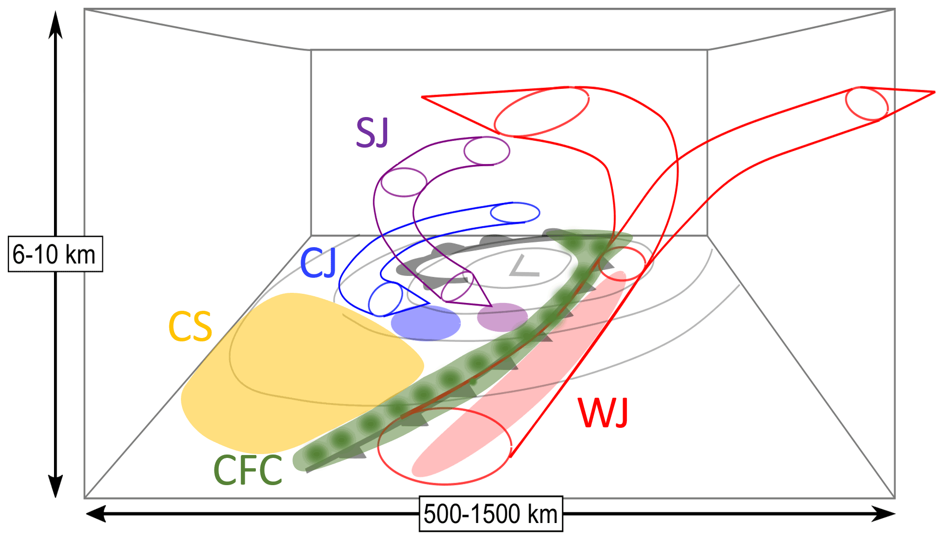
Figure 1 Conceptual model of the 3D structure of a SKC showing the WJ (red), CJ (blue) and SJ (magenta). In each case, the region of strong surface winds is indicated by an ellipse. The figure and caption have been adapted from (Clark and Gray, 2018; their Fig. 7) to include the CFC (green) and CS (gold).

All features can cause damage due to strong gusts; thus, it is important to accurately forecast them and their associated wind fields. A widely employed approach to improve forecasts (not only of wind) is statistical post-processing (Vannitsem et al., 2021), during which the model output is corrected on the basis of past forecast errors. The performance of various ensemble post-processing methods for wind gusts has been discussed in a recent paper by Schulz and Lerch (2022), who found that approaches ranging from classical statistical methods to novel neural-network-based techniques significantly improve forecast reliability and accuracy. However, Pantillon et al. (2018), who applied one of the classical statistical methods to ensemble forecasts of wind gusts and analysed the performance for several winter storms over Germany, found that post-processing can actually considerably worsen the forecast in some cases, as it did, for example, for storm Christian (October 2013), which is known to have developed an SJ (Browning et al., 2015). Similar results were also found for storm Friederike in January 2018 (not shown). This can generally come from a “misprediction” of the cyclone track or intensity but could also indicate that the characteristics of individual mesoscale high-wind features are not well represented. If that was the case, a feature-dependent post-processing could lead to further improvement, as it could consider the specific dynamical characteristics and how they are treated in the forecast model. By developing an objective identification algorithm for the wind features shown in Fig. 1, this work lays the foundation for further exploring this idea.

Hewson and Neu (2015) analysed observations and reanalysis data of 29 wind storms with a focus on the three low-level jets: WJ, CJ and SJ. They included CFC in their WJ analysis instead of treating it as an independent feature. They showed that the three wind features differ in their location of occurrence relative to the cyclone centre, in their timing within the cyclone life cycle, and in their duration, strength and surface footprint, among others. Furthermore, Earl et al. (2017) looked at the most common causes of high surface gusts in UK extratropical cyclones and, besides WJ, CJ and SJ, included several convection-induced high-wind features. They based the identification of SJs on satellite images, the location of the gusts within the cyclone and the deepening rate. As no confirmation with Lagrangian trajectory analysis was done, the identified features are referred to as “potential SJs”. Earl et al. (2017) found that, although WJs and CJs are the most common causes of high winds, the strongest gusts are caused by CFC and potential SJs. Parton et al. (2010) categorised strong wind events captured by a wind-profiling radar in Wales over a 7-year period into cold frontal events (similar to our definition of CFC), warm-sector winds (similar to WJ), tropopause folds/warm fronts, SJs and unclassified events. They found that warm-sector events were the cause of around 40 % of all strong winds, followed by cold frontal events (around 24 %).

As all of these approaches are purely subjective, relatively time-consuming and, thus, hard to automate, we aim to develop an objective analysis of the different mesoscale wind features that can flexibly be applied to station and gridded data and, therefore, serve as a basis for climatological studies, forecast evaluation and post-processing development. The strategy that we follow is to start with a subjective identification (as in previous studies) but to use the results to then train a probabilistic random forest (RF) to develop an objective procedure that can be applied to cases outside of the training data set. The identification is designed to be independent of horizontal gradients (and hence resolution) and can principally be applied to observations from a single weather station. In addition, the identification is based on tendencies over 1 h only, making it applicable to time series with gaps. Our newly developed method is referred to as RAMEFI (RAndom-forest-based MEsoscale wind Feature Identification). Given that the provision of such a feature-dependent post-processing tool can enhance the forecasts of strong winds and wind gusts, it can potentially contribute towards better weather warnings and impact forecasting of such events (e.g. Merz et al., 2020). In this paper, we will show examples using surface stations and Consortium for Small-scale Modeling (COSMO) reanalysis data. A full long-term climatology is the focus of Part 2 of this paper (Eisenstein et al., 2022d). The output of the RF are feature probabilities, rather than binary identification, which allow for an evaluation of how well individual data points fit the typical feature characteristics as well as the identification of hybrid features or transition zones.

The paper is structured as follows: a short description of each wind feature is given in Sect. 2, based on results from previous studies; the used data sets and methods are discussed in Sect. 3; Sect. 4 details our new software RAMEFI, starting from the subjective labelling of wind features through the training of the RF to the display of areal feature information; Sect. 5 illustrates our approach with a case study; a statistical evaluation of the performance of the RF can be found in Sect. 6; strengths and weaknesses of the approach are discussed on the basis of specific case studies in Sect. 7; and Sect. 8 summarises our work and discusses future plans.

2 Characteristics of high-wind features

In this section, the most important high-wind features within extratropical cyclones are shortly described on the basis of the existing scientific literature. Figure 1 exemplarily shows a typical SKC; differences to an NC are discussed in the following. While WJs and CJs are common to both cyclone models, SJs can only occur in SKCs (Clark and Gray, 2018). On the other hand, SKCs are rarely accompanied by (strong) CFC, as their cold front is often weak (Schultz et al., 1998). The following descriptions of individual features are mostly based on Hewson and Neu (2015), Earl et al. (2017), and Clark and Gray (2018). For more details, the reader is referred to these publications.

2.1 Warm jet

An important feature in extratropical cyclones is the warm conveyor belt (WCB;  Wernli and Davies, 1997; Eckhardt et al., 2004; Madonna et al., 2014). It starts near the surface ahead of the surface cold front and later ascends above it. During the ascent, the WCB splits into a cyclonic and anticyclonic branch as seen by the red tubes in Fig. 1. While the cyclonic part forms the cloud head and usually causes heavy precipitation along a narrow region, the anticyclonic part rises above the warm front and causes more moderate precipitation over a wider area. Overall, the WCB is the main cause of long-lasting precipitation (Catto, 2016). Furthermore, the WCB can be the cause of strong convection along the cold front (Hewson and Neu, 2015).

Here, we focus on the early stages of the WCB while it is still near the surface and can cause high winds there, and we refer to it as the warm jet (WJ). Contrary to Hewson and Neu (2015), we define the WJ as the region ahead of the cold front and its convection, and hence ahead of the CFC feature (see Sect. 2.4), as displayed by the red shaded ellipse in Fig. 1. Located in the warm sector of the cyclone between the two rain-active fronts, the WJ is usually characterised by positive temperature anomalies, decreasing pressure with time, and little or no precipitation. The WJ is usually associated with the first strong winds starting in an early stage of a cyclone. Maximum gusts of around 25 m s⁻¹ are typical (Hewson and Neu, 2015). As the warm conveyor belt is an ascending airstream, the winds at the surface weaken and disappear in later stages when the warm conveyor belt no longer affects the boundary layer. The jet is long-lived with a duration of 24 to 48 h and can cause a large surface wind footprint with a width of 200 to 500 km and a length of up to 1000 km (Hewson and Neu, 2015). While the predictability was evaluated to be good with a relatively high coherence in space and time, Hewson and Neu (2015) found that the occurrence of very high winds within the warm sector was rather unusual, whereas Parton et al. (2010) associated 40 % of strong wind events with winds within the warm sector. Such a seeming contradiction can potentially be resolved with a climatological application of the identification algorithm that we have developed in this paper. Due to generally stable conditions in the warm sector, wind speeds above the boundary layer are usually much higher than surface gust speeds. Compared with the CJ and SJ, the WJ is the most long-lasting, but – as already mentioned – it typically does not cause the most destructive winds.

2.2 Cold jet

The CJ is associated with the main airflow of the cold conveyor belt that turns cyclonically around the centre of the low (blue tube in Fig. 1). At first, the CJ moves around the north-western flank behind the occluded or bent-back front beneath the cloud head. As it is travelling against the motion of the low-pressure system, the CJ is hard to see in Earth-relative winds until it wraps around the cyclone centre. Once wrapped around, the CJ can cause strong surface gusts near the tip of the front, as shown by the blue shaded ellipse in Fig. 1. This usually happens around the time the maximum intensity is reached. The CJ weakens when the low decays or shortly before that. The jet mainly stays close to the ground, i.e. below 850 hPa (Smart and Browning, 2014), or ascends slightly during its life cycle (Martínez-Alvarado et al., 2014). With typical maximum gusts of around 30 m s⁻¹, the CJ is stronger than the WJ but, with a typical lifetime of 12 to 36 h, does not last as long (Hewson and Neu, 2015). The impacted area expands with time, while the cold conveyor belt (and hence the CJ) wraps around the cyclone centre when the footprint can finally reach a width of around 100 to 800 km and a length of up to 2500 km (Hewson and Neu, 2015). Although forming later in the life cycle of the parent cyclone than the SJ, both jets can coexist. A damaging CJ is more common than an the SJ or WJ over Europe (Hewson and Neu, 2015).

2.3 Sting jet

The SJ is a distinct airstream that descends from mid-levels within the cloud head into the frontal fracture region of an SKC (magenta tube in Fig. 1). When the CJ wraps around the low, the SJ can be replaced by the CJ or merge with it. Hewson and Neu (2015) suggest an average surface footprint of less than 100 km in width and up to 800 km in length. SJs usually last just a few hours but can be active for up to 12 h in extreme cases. A detailed review can be found in Clark and Gray (2018). The most common way to identify SJs is to compute Lagrangian trajectories (e.g. Volonté et al., 2018; Eisenstein et al., 2020), for which a high resolution is required, horizontally and vertically as well as temporally. Recent work has tried to identify SJs using low-cost approaches. For example, Gray et al. (2021) introduced an instability-based precursor tool, while Manning et al. (2022) developed a kinematic approach looking for reversals in the vertical gradient of horizontal wind speed along streamlines.

2.4 Cold frontal convection

The passage of cold fronts is often accompanied by heavy precipitation, sometimes in the form of convective lines, which, in turn, can cause strong wind gusts associated with the downward transport of high momentum from above the boundary layer. CFC is displayed in Fig. 1 as an elongated line along the front with several darker spots representing individual convective events. Cold-front-related rain, snow and graupel are responsible for around 28 % of extreme precipitation events in the midlatitudes (Catto and Pfahl, 2013). The frontal zone is characterised by a marked change in wind direction and a decrease in temperature (Clark, 2013). In extreme cases, tornadoes can occur in association with CFC, causing even more hazardous winds (e.g. storm Kyrill; Fink et al., 2009). Earl et al. (2017) suggest a separation of CFC into convective lines and pseudo-convective lines. The latter do not strictly satisfy identification criteria for convective lines but show characteristics of organised, strong convection and may fulfil the criteria earlier or later. A convective line shows a clear signal in radar imagery at 3 to 10 km height (Parton et al., 2010). In the case of a kata cold front, CFC occurs at and ahead of the surface cold front (Lackmann, 2011). Although high winds might then, strictly speaking, occur within the warm sector, we have decided not to associate these high winds with the WJ due to their physically distinct characteristics. In case of an ana cold front, CFC occurs at and behind the cold front, and the distinction is therefore more straightforward. SKCs usually have a rather weak cold front; hence, high winds are less likely to be associated with CFC (Schultz et al., 1998).

2.5 Cold-sector winds and post-cold-front convection

The cold sector is the region behind the cold front (gold shading in Fig. 1). In this area, high winds can be caused by post-cold-front convection as well as by a so-called “dry intrusion”. This region of a cyclone is generally known for its instability and turbulent behaviour. A dry intrusion is, as for an SJ, a descending airstream; however, in this case, it is one that originates near the tropopause or even in the lower stratosphere. Thus, it transports dry air down to the middle and lower troposphere moving towards the cyclone centre (Raveh-Rubin, 2017). Dry intrusions – and, later in the cyclone's life cycle, a dry slot near the cyclone centre – can often be seen in water vapour satellite imagery. Raveh-Rubin (2017) state that dry intrusions can cause destabilisation and increased wind gusts. Furthermore, cold fronts show a stronger temperature gradient, higher winds and more precipitation when accompanied by a dry intrusion (Catto and Raveh-Rubin, 2019; Raveh-Rubin and Catto, 2019). Most publications consider all high winds on the colder side of a cyclone to be a CJ or SJ and do not distinguish these features from other cold-sector winds (e.g. Manning et al., 2022). Given the relatively large area of the cold sector in many cyclones and the appearance of discernible substructures, we decided to specifically separate out CFC, CJ and SJ here and then label the remaining strong winds as CS.

3 Data and method

This section introduces the observation and gridded data sets as well as 12 winter storm case studies used for the training and evaluation of RAMEFI. Furthermore, it describes how to assess the probability predictions obtained by the RF.

3.1 Surface observations

The main basis of our analysis is a data set of hourly surface observations from 2001 to mid-2020. This includes mean sea level pressure (p), 2 m air temperature (T), wind speed at 10 m (v), wind direction at 10 m (d) and precipitation amount (RR). Using T and p, we further compute the surface pressure using the barometric height formula to then calculate the potential temperature (θ). Our focus is on Europe – more specifically, stations within the area from −10 to 20 ^∘ E and from 40 to 60 ^∘ N. Around 1700 stations are included; however, of these aforementioned stations, less than 400 stations on average observe all five parameters. For the training of the RF (Sect. 4), we focus on stations that measure at least three of the five parameters. The most frequent missing parameter in the hourly data is RR, as many stations only measure 3- or 6-hourly precipitation. However, many stations, especially over Germany, measure RR only and, hence, are not usable for the training of the RFs (Sect. 4.2); nevertheless, they are still helpful to inform our subjective labelling (Sect. 4.1). In addition, we exclude mountain stations, i.e. those with a station height above 800 m, as we suspect these to be dominated by orographic influences that may blur the feature characteristics that we want to identify. This leaves around 750 stations per time step.

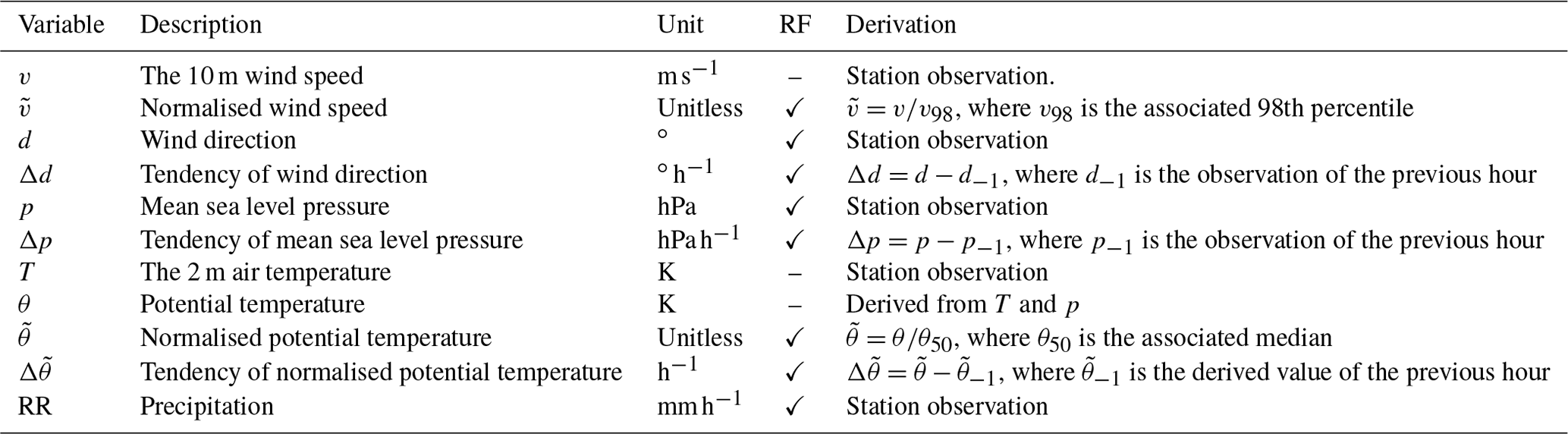
In order to take the diurnal and seasonal cycles as well as location-specific characteristics (e.g. exposed stations in coastal regions) into account in θ and v, we decided to normalise these parameters by their climatology. For θ, this means $\stackrel{\mathrm{̃}}{\mathit{\theta }}=\mathit{\theta }/{\mathit{\theta }}_{\mathrm{50}}$, where θ₅₀ is the median for the specific location, time of day and day of the year ±10 d. This is done analogously for v using the 98th percentile, $\stackrel{\mathrm{̃}}{v}=v/v_{\mathrm{98}}$, as we are mostly interested in high winds in this work. The 98th percentile is used in analogy to standard high-wind quantities such as the storm severity index (SSI), which is computed from stations where measured gusts exceed the local 98th percentile and provides an integral indication of the strength of the cyclone and the associated potential damage (see Appendix A for details). Both θ₅₀ and v₉₈ are computed for the time period from 2001 to 2019. Moreover, we are interested in temporal tendencies of p, $\stackrel{\mathrm{̃}}{\mathit{\theta }}$ and d, here represented simply by the difference between the current and the prior time step (Δp, $\mathrm{\Delta }\stackrel{\mathrm{̃}}{\mathit{\theta }}$ and Δd respectively). All parameters and their descriptions are listed in Table 1.

Table 1 Overview of the variables considered for the objective identification using the probabilistic RF. The fourth column indicates whether the variable is used as an input variable for the final version of the RF. The associated percentiles and medians are computed with respect to the location, time of day and day of the year ±10 d.

3.2 COSMO-REA6

As an example of a gridded data set, we use COSMO-REA6 data from the Hans-Ertel-Centre for Weather Research, which are a reanalysis based on the COSMO model from the German Weather Service (DWD) covering the European CORDEX domain with a grid spacing of 0.055 ^∘, i.e. roughly 6 km (Bollmeyer et al., 2015). Several parameters, including wind, temperature, humidity and pressure, are assimilated using a nudging technique. Observations from radiosondes, aircraft, wind profilers and surface stations are used for the nudging. However, precipitation is not assimilated, which can lead to larger deviations between the reanalysis and rain gauge or radar observations (Bach et al., 2016; Hu and Franzke, 2020). The reanalysis is available from 1995 to 2019. This means that one of our case studies, namely storm Sabine, is not included (Table 2). The same surface parameters as mentioned in Sect. 3.1 are used. The data set contains p, T, RR, and the zonal and meridional wind components, from which we can compute v and d. Again, we further calculate $\stackrel{\mathrm{̃}}{\mathit{\theta }}$ and the temporal tendencies Δp, $\mathrm{\Delta }\stackrel{\mathrm{̃}}{\mathit{\theta }}$ and Δd. Due to the computational cost, we compute θ₅₀ and v₉₈ for the 10-year time period from 2005 to 2015 only, but this should have a negligible effect on the final outcome. The data, originally on a rotated grid, are regridded to a latitude–longitude grid with a grid spacing of 0.0625 ^∘, i.e. roughly 7 km, for the area from −10 to 30 ^∘ E and from 40 to 65 ^∘ N.

3.3 Case studies

In this work, we focus on 12 winter storm case studies between the years 2015 and 2020, as listed in Table 2. The selection was based on their SSI over Germany (see Appendix C), the damage caused and the area impacted. This includes the eight winter storms with the highest SSI during this time period as well as four subjectively chosen more moderate storms to capture a healthy diversity of cyclones and features. The selected cases occurred during the extended winter half-year between the end of September and the end of March. They vary in terms of their cyclone tracks (Fig. 2) and their high-wind features, and they include both NCs and SKCs. Two case studies developed SJs, namely Egon (Eisenstein et al., 2020) and Friederike. We also include two storms, named Herwart and Sabine, with an exceptional large pressure gradient leading to a stronger background wind field, such that it is more difficult to distinguish the features and the contribution of them to the storm's wind footprint. Further, Sabine stands out as an extremely deep cyclone with a minimum core pressure of 944 hPa during its lifetime.

Table 2 Selected winter storm cases from 2015 to 2020 over central Europe, showing the name (as given by the Free University of Berlin), date, maximum observed gust speed (location), SSI over Germany and associated high-wind features including exceptional large pressure gradients (SPG). The cyclone tracks are displayed in Fig. 2.

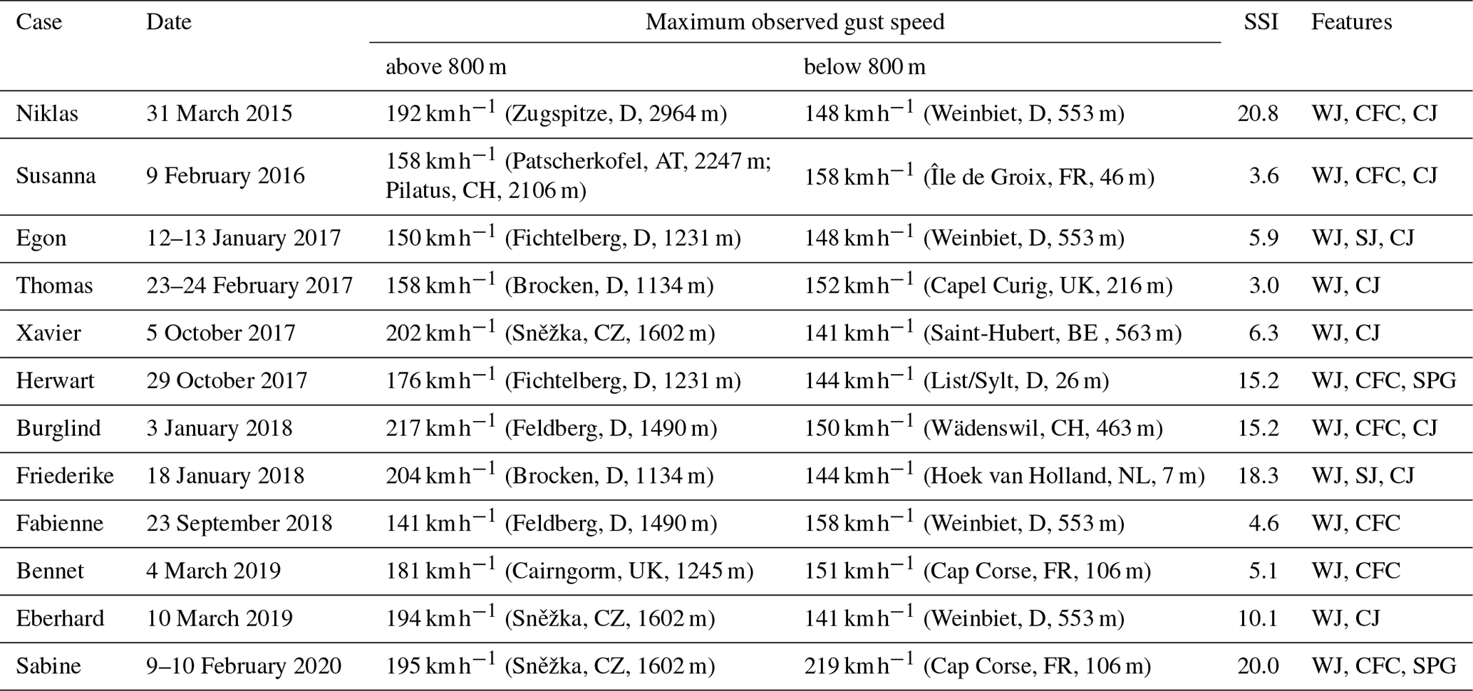
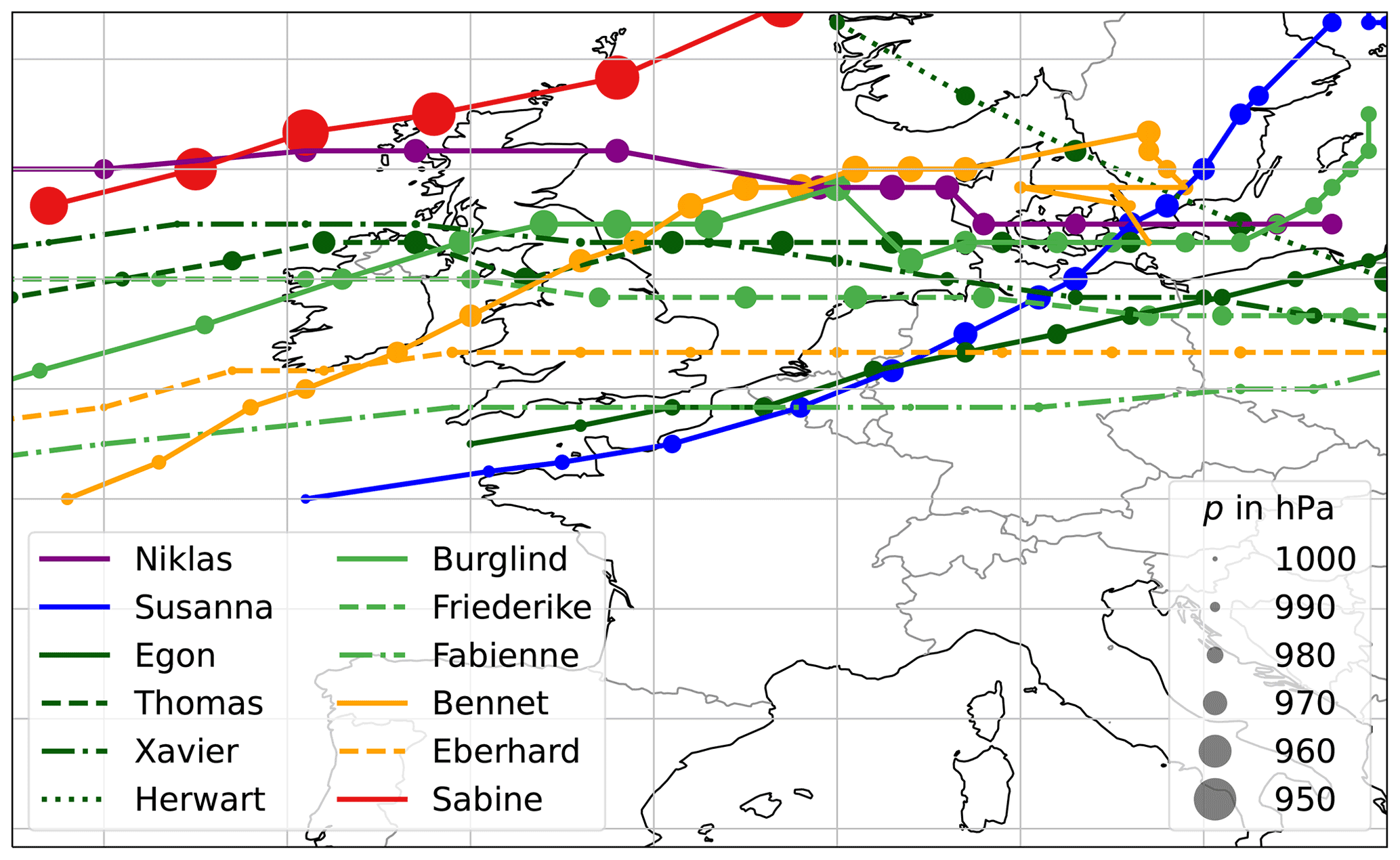
Figure 2 Cyclone tracks of case studies from Table 2. Colour indicates the year (purple – 2015, blue – 2016, dark green – 2017, green – 2018, orange – 2019 and red – 2020), and the line style indicates the order of occurrence in that year (solid – dashed – dot-dash – dotted). The size of the markers corresponds to the minimum mean sea level pressure (p).

3.4 Assessing probability predictions for multiple wind features

Probability predictions of three or more classes, such as the wind features, are typically evaluated by downscaling to two-class problems, of which the one-against-all and all-pairs approaches are two well-known examples (Zadrozny and Elkan, 2002). While the one-against-all approach compares the occurrence of one wind feature against all others grouped together, the all-pairs approach considers the conditional probabilities of each pair of classes – for example, the conditional probabilities of the WJ and the CJ when one of the two features materialises. The one-against-all approach is used to evaluate how well one specific wind feature is predicted, whereas the all-pairs approach is used to evaluate the ability to discriminate between two wind features.

The probabilities are evaluated based on the paradigm of Gneiting et al. (2007) that a prediction should aim to maximise sharpness subject to calibration. Calibration refers to the consistency of the prediction and the observation, while sharpness is a property of the prediction alone and refers to the associated uncertainty. In a nutshell, a probability f is called calibrated if the conditional event probability (CEP; conditional on f) matches f; for example, if a 20 % prediction is issued 100 times, the event should occur about 20 times. Further, a probability prediction is said to be sharper, the more confident the prediction is – that is, the closer to zero or one. Both calibration and sharpness can be assessed qualitatively via reliability diagrams, which display the calibration curve (Sanders, 1963; Wilks, 2011). The calibration curve is a plot of the CEP dependent on the probability f, which is close to the diagonal if the predictions are calibrated. In addition to the calibration curve, the frequency of the probabilities is illustrated by a histogram. The more U-shaped the histogram, the closer the predictions are to zero and one and, thus, the sharper the prediction. The reliability diagrams shown in this paper are based on the novel CORP (consistency, optimality, reproducibility, pool adjacent violators (PAV) algorithm) approach of Dimitriadis et al. (2021), which yields optimal calibration curves and eliminates the need for implementation decisions for the calculation of the calibration curve.

Quantitatively, calibration and sharpness can be assessed using the Brier score (BS; Brier, 1950): the lower the score, the better the prediction. Here, we compare our RF probabilities with the class frequencies observed in the training data of the RF using the Brier skill score (BSS), which denotes the improvement of the RF over a prediction based on the class frequencies in the RF training data, where a negative percentage corresponds to worse predictions, 0 % corresponds to no improvement and 100 % corresponds to an optimal prediction. Details on the evaluation of probability predictions are provided in Sects. B1 (practical implementation) and C1 (mathematical formulation) in the Appendix.

4 RAMEFI

Our new method, RAMEFI, focuses on strong but not exceptionally high wind speeds. These wind speeds are usually indicated by the 98th percentile. To obtain a sufficiently large storm area and to base that on a widely used reference, we decided to include stations reaching 80 % of their 98th percentile, i.e. $\stackrel{\mathrm{̃}}{v}\ge \mathrm{0.8}$. To capture usually narrow and fast-moving features such as CFC, RAMEFI requires hourly data. All used parameters are independent of the location of the station/grid point and horizontal gradients; hence, in principle, the approach can be applied to a single station and to data sets with differing horizontal resolution. The approach evaluates each 1 h interval independently.

RAMEFI includes three steps described in the following subsections: (1) we subjectively identify the features in surface observations in 12 selected case studies, such that each station is assigned to a specific feature; (2) these labels are then used to train RFs for feature prediction on the basis of a cross-validation approach; and (3) we obtain predictions on a grid by interpolating the predicted probabilities using a Kriging approach. For the COSMO-REA6 data, the features are identified analogously. Instead of training separate RFs, we apply the RFs trained on the surface observations. As the COSMO-REA6 forecasts are already grid-based forecasts, the Kriging step is obsolete.

4.1 Subjective labelling using an interactive tool

Given the sometimes unclear distinction between the high-wind features of interest in realistic cases, we decided to base our algorithmic development on how experienced meteorologists would identify the features on the basis of a wide range of parameters and their evolution in time and space. To accelerate and facilitate the subjective labelling of high-wind features, we developed an interactive tool using the open-source Bokeh (Bokeh Development Team, 2021) data visualisation package for Python, where one can switch between the available parameters (Table 1) in a graphical display and select an area to set labels using a mouse-controlled lasso tool. A screenshot is provided in Appendix D (Fig. D1).

The guiding principles for the labelling were extracted from the scientific literature (see Sect. 2) and are mainly based on the location relative to the cold front and cyclone core. For this, analysis charts of the DWD and the UK Met Office were used for orientation. For a more detailed analysis, we also used the 3D front detection of the Met.3D interactive visualisation software (Beckert et al., 2022; Rautenhaus et al., 2015). In our surface parameters, a cold front is then mostly identified through the characteristic change of the sign of Δp. It is labelled CFC if a larger area of precipitation along it is observed, while high winds ahead of the front within the warm sector are labelled WJ. The CJ is mostly detected through its hook-shaped wind footprint at the tip of a wrapped-around occlusion or bent-back front as well as through its proximity to the cyclone centre. An SJ is labelled when model-based trajectories analogous to Eisenstein et al. (2020) confirm a descending airstream. The area behind the cold front that is not associated with the CJ or SJ is labelled as the CS. An example of the reasoning behind the labelling is described for one time step of storm Burglind in Sect. 5.

The subjective labelling was done for the introduced 12 extratropical cyclone case studies (see Sect. 3.3). In total, 282 time steps have been analysed. As mentioned above, we excluded mountain stations and stations where less than three of the given parameters were measured. This leaves around 750 stations per time step for the subjective labelling. Overall, for the 12 case studies, we have 77 517 data points where $\stackrel{\mathrm{̃}}{v}\ge \mathrm{0.8}$, of which 19 200 (24.77 %) are not associated with a feature (NF), 21 809 (28.13 %) were labelled as CS, 19 501 (25.16 %) were labelled as WJ, 11 705 (15.1 %) were labelled as CJ, 3800 (4.9 %) were labelled as CFC and 1502 (1.94 %) were labelled as SJ. However, the SJ is a small, short-lived and rare feature, and the characteristics of SJs and CJs in surface parameters are very similar due to the proximity in both time and space. A first training with SJ and CJ as separate features showed that a clear distinction is not possible with the information at hand and that the SJ is mostly detected as CJ. Therefore, we decided to include it in the more frequent CJ feature, increasing the values for CJ to 13 207 data points (17.04 %).

The features were further labelled in all case studies (except for storm Sabine, which occurred outside of the reanalysis time period) using the interactive tool for COSMO-REA6 data. These labels are used to evaluate the predictions generated by the station-based RFs for a grid-based data set (Sects. 4.2 and 6.1). For computational reasons, i.e. as labels are set for every grid point rather than an area, we downsampled the COSMO grid to every third grid point in the zonal and meridional directions, resulting in a grid spacing of 0.1875 ^∘ (i.e. around 21 km). Moreover, we excluded ocean grid points, as the characteristics of the high-wind features might be different from land due to different surface friction and surface heat fluxes, among other factors. Regions with a high wind speed not directly associated with a winter storm, especially over Italy and the Balkans, were not labelled.

4.2 Probabilistic random forest

RF (Breiman, 2001) is a popular, robust machine learning method for classification and regression problems that does not rely on parametric assumptions but is instead based on the idea of decision trees (Breiman, 1984). Given data for which we want to generate predictions, a decision tree operates by assigning each sample to one of its so-called leaves, which is done by subsequent queries at the so-called nodes, where we check whether one of the input variables exceeds a certain threshold. Each leaf is associated with that subset of the training data that satisfies the criteria of the corresponding nodes. Tailored to the specific task, a prediction is then derived from the associated subset. Here, we obtain probability predictions by using the frequencies of the observed wind features among the samples in the corresponding leaf. The queries at the nodes, i.e. the specific input variables and corresponding thresholds, are chosen automatically such that the terminal leaves are as diverse as possible. The maximal depth, the minimal node size and the diversity criterion are tuning parameters and can be chosen by the user. An RF builds a randomised ensemble of decision trees, where the generation of each tree is based on a different subsample of the training data, and the generation of each node is based on a different subset of input variables. To obtain a final prediction from the ensemble, the individual predictions of the decision trees are aggregated. For further details on RFs, we refer to Breiman (2001) and Hastie et al. (2009). In a meteorological context, probabilistic RFs have already been applied to predict damaging convective winds (Lagerquist et al., 2017) and severe weather (Hill et al., 2020) as well as in a general form for a wide range of applications such as ensemble post-processing of surface temperature and wind speed (Taillardat et al., 2016).

Machine learning methods such as RF are often referred to as “black boxes” due to a lack of interpretability, although several techniques exist to understand what the models have learnt and how the predictions are related to the input variables, typically referred to as predictors (McGovern et al., 2019). We will apply two of these predictor importance techniques: one to find the most relevant predictors and one that illustrates the effect of the predictor values on the RF probabilities. The first is the permutation importance of a predictor (Breiman, 2001). Proceeding separately for each predictor, the values of that predictor are shuffled randomly within the test data in space and time such that the physical relation to the observed wind feature is broken. Then, based on these permuted predictor values, new predictions are generated and compared to those obtained with the original data. The worse the predictions become (with respect to an evaluation measure), the more important the predictor. Here, we measure predictive performance with the BS that was introduced in Sect. 3.4, and the importance measure is referred to as BS permutation importance. The second technique is given by the partial dependence plot (PDP; Greenwell, 2017), which illustrates the effect of a predictor on the prediction. Given a fixed predictor, a PDP shows the expected RF probability dependent on the value of the predictor variable while averaging out the effects of the other predictors. Hence, a PDP illustrates how the RF probabilities depend on the value of a specific predictor variable, on average. For more details, we refer to McGovern et al. (2019).

In this study, we apply RFs to generate probabilities of the wind features presented in Sect. 2. The input variables used are listed in Table 1. For the station-based observations, we use a cross-validation scheme on the different winter storm cases – that is, for each winter storm, the predictions are generated by an RF that is trained on the data of the remaining 11 winter storms. Training RFs in a similar cross-validation scheme for the COSMO-REA6 data becomes computationally infeasible, as the underlying data sets become too large. As the underlying processes should coincide for both the station- and model-based data, we instead apply the station-based RFs in the same scheme to generate probabilities using the COSMO-REA6 data. Details on the implementation, including the choice of the tuning parameters, can be found in Appendix B2.

Due to normalising θ and v, the trained RF is fairly independent of location-specific information, such that it can hopefully be applied successfully to other midlatitude regions around the world affected by extratropical cyclones. However, before doing that, we recommend a thorough sanity check, particularly when using it over the ocean and mountainous regions.

4.3 Kriging

As it is difficult to envision a coherent area of a certain wind feature from probabilities at single stations that are distributed irregularly over the study area, we interpolate the station-based probabilities to a regularly spaced grid in order to visualise the results. In geostatistics, this is generally achieved by Kriging (Matheron, 1963). In principle, the Kriging predictions (here, on the grid) are the weighted averages of the input data (here, the station data), where the specification of the weights is driven by the covariance of the underlying random process. Under the assumption of Gaussianity (Rasmussen and Williams, 2005), Kriging provides the optimal full predictive distribution. The key requirement for the implementation of Kriging in the context of Gaussian processes is the specification of the mean and the covariance function.

In this study, we perform univariate Kriging to obtain probability maps for each wind feature, where we specify the mean and covariance function by a constant mean function and the stationary Matérn covariance function (Matérn, 1986; Guttorp and Gneiting, 2006). For the estimation, we resort to the method of maximum likelihood estimation for Gaussian processes. However, as the input data are, in our case, probabilities and, thus, deviate from the Gaussianity assumption, we perform a data transformation for approximate Gaussianity. For the production of probability maps, we independently perform Kriging on each of the class probabilities (hence univariate Kriging) and normalise the resulting probabilities for each grid point such that, across the multiple wind feature, the probabilities sum to one. Note that the Kriging predictions are only obtained for areas over land, where our winter storms occurred and where a sufficient amount of data was available for a reliable interpolation. More details regarding the Kriging approach are provided in Sects. B3 (practical implementation) and C2 (mathematical formulation) in the Appendix C.

5 Illustrative case study: storm Burglind

In this section, a full case study for storm Burglind is presented to illustrate the functionality of the new RAMEFI feature detection method. Burglind is relatively close to a “textbook” cyclone and shows a feature evolution largely in concordance with the literature.

5.1 Synoptic evolution

Storm Burglind (also known elsewhere as Eleanor) developed as a secondary cyclone on 2 January 2018 over the North Atlantic and reached the British Isles at the end of that day. The core pressure dropped by more than 27 hPa in 24 h and, thus, exceeds the criteria for an explosive cyclogenesis after Sanders and Gyakum (1980). The minimum pressure occurred just east of the English North Sea coast around 03:00 UTC on 3 January. The cyclone then tracked mostly eastward across the North Sea and Baltic Sea before heading northeastward in later stages (Fig. 2). The cold front crossed France and Germany in the first half of 3 January and caused high winds due to CFC. Ahead of the front, high winds were associated with the WJ. Later, when the occlusion front wrapped around the cyclone centre, the CJ dominated as the cause of high winds in addition to CS winds further away from the cyclone core.

5.2 Application of feature identification

Figure 3 shows the most important parameters, namely p, RR and $\mathrm{\Delta }\stackrel{\mathrm{̃}}{\mathit{\theta }}$, to distinguish the high-wind features for one selected time step, i.e. 3 January 2018 at 06:00 UTC, to illustrate the subjective labelling process, as described in Sect. 4.1. The cyclone centre was located to the east of the UK over the North Sea (red “x” in Fig. 3). The cold front stretched from north-western Germany to France (see Fig. D4 in Appendix D). The highest winds were observed ahead of and along the cold front and over western France (contours in Fig. 3). Figure 3a shows p decreasing strongly with values of mostly above 3 hPa over southern and eastern Germany ahead of the cold front. The increase after the front is a lot weaker with some stations even still showing a weak decrease, which can, for example, be caused by small-scale processes like convection. Nevertheless, coinciding with the location of the front, several stations observe a p increase of around 2 hPa. This region also coincides with areas of heavy rain, with values of around 5 mm h⁻¹ to more than 8 mm h⁻¹ (Fig. 3b). Slightly lower amounts were observed along the occluded front and northern part of the warm front. Furthermore, we note a change in $\stackrel{\mathrm{̃}}{\mathit{\theta }}$ (Fig. 3c), with an abrupt decrease in the frontal region and a shift of d from south-westerly to westerly winds (not shown). While $\mathrm{\Delta }\stackrel{\mathrm{̃}}{\mathit{\theta }}$ indicates large tendencies over northern France and western Germany, it shows noisier behaviour further away from the highest winds. Following this, we set labels for a WJ in the region of negative Δp, positive $\mathrm{\Delta }\stackrel{\mathrm{̃}}{\mathit{\theta }}$ and ahead of the high values of RR. CFC is labelled in the frontal region, where the heavy precipitation occurred. As the occluded front is not wrapped around the core yet (cf. Fig. D4), implying that a CJ is not yet occurring at this point in time, the region behind the cold front is entirely labelled as CS. All set labels are displayed in Fig. 3d.

Figure 3 Storm Burglind on 3 January 2018 at 06:00 UTC. Scattered dots show station observations for (a) Δp, (b) RR, (c) $\mathrm{\Delta }\stackrel{\mathrm{̃}}{\mathit{\theta }}$, and (d) subjectively identified wind features for stations where $\stackrel{\mathrm{̃}}{v}\ge \mathrm{0.8}$ and at least three of the five initial parameters are measured (see Sect. 4.1). The contours show the interpolated $\stackrel{\mathrm{̃}}{v}$ (dotted $\stackrel{\mathrm{̃}}{v}=\mathrm{0.8}$, dashed $\stackrel{\mathrm{̃}}{v}=\mathrm{1}$ and solid $\stackrel{\mathrm{̃}}{v}=\mathrm{1.2}$) to display the regions where the highest winds occurred. The red “x” indicates the cyclone centre.

The predictions of feature probabilities by the RF, which is trained on the 11 other cases (Table 2), for 06:00 UTC and other time steps at a 3 h interval are shown in Fig. 4 after Kriging was applied to generate a gridded field of probabilities. Moreover, $\stackrel{\mathrm{̃}}{v}$ and p contours are added for orientation. An animation for the entire lifetime of Burglind is provided in the video supplement (Eisenstein et al., 2022c).

Comparing Fig. 3d (subjectively identified features) and Fig. 4b (RF predictions) shows that the features are mostly in consistent areas with high confidence. CFC is identified in a smaller region, which is partly due to missing precipitation observations, because this is the most important variable to predict CFC, as will be discussed in Sect. 6.2.

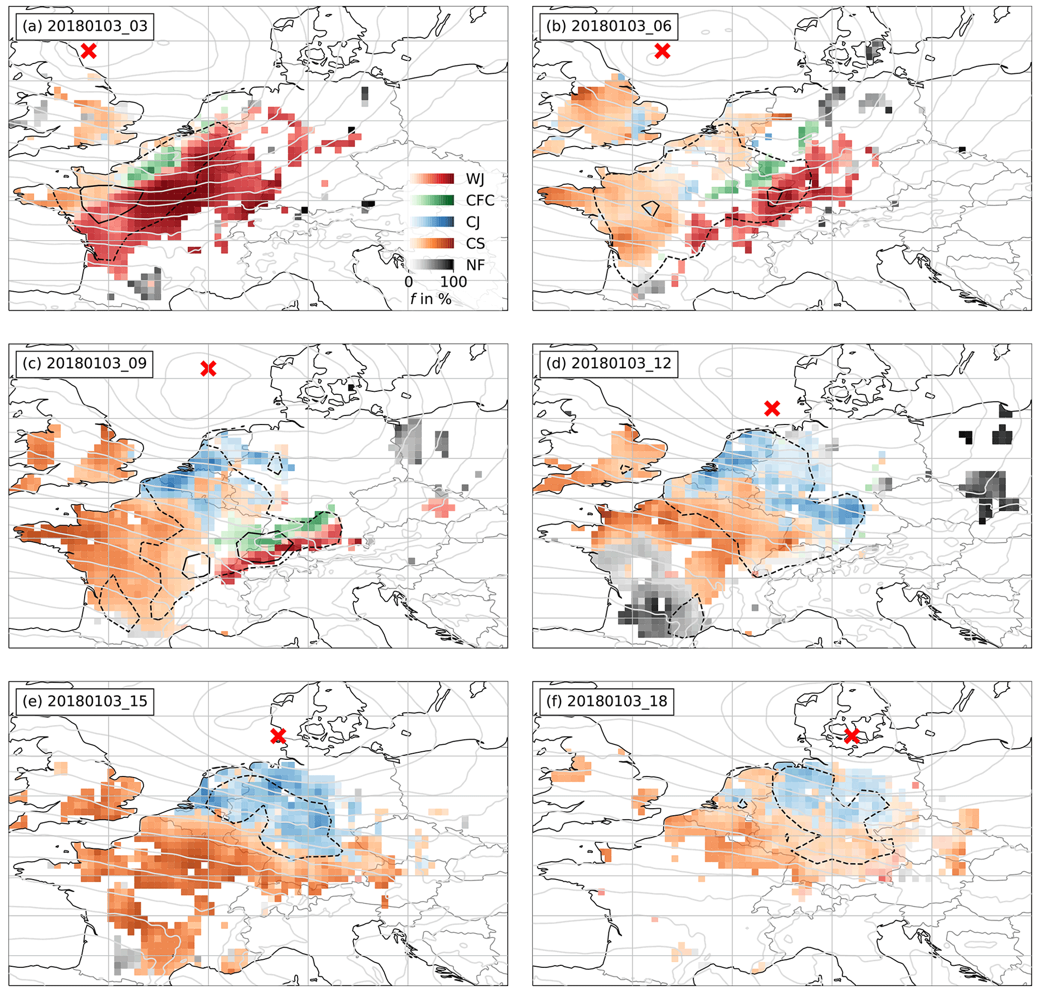
Figure 4 RF probabilities f for each high-wind feature after Kriging for storm Burglind on 3 January 2018 at (a) 03:00 UTC, (b) 06:00 UTC, (c) 09:00 UTC, (d) 12:00 UTC, (e) 15:00 UTC and (f) 18:00 UTC. The dashed contour shows $\stackrel{\mathrm{̃}}{v}=\mathrm{1}$, and the solid contour shows $\stackrel{\mathrm{̃}}{v}=\mathrm{1.2}$. The red “x” indicates the cyclone centre. Light grey contours show COSMO-REA6 p with a 4 hPa interval.

As stated, the WJ is the first feature to occur during the life cycle of a cyclone, as is the case for Burglind. Figure 4a shows the 3 January 2018 at 03:00 UTC, when high probabilities of a WJ are predicted for most of central France. This region is followed by a smaller region of CFC along the front and CS behind it. As the cyclone evolves further, the cyclone centre and the identified features coherently move further east, while the area affected by the WJ diminishes (Fig. 4b). A total of 3 h later the WJ dissolves north of the Alps while still being followed by a line of identified CFC (Fig. 4c). At this time step, which is also the time of minimum core pressure, the CJ is identified on the coasts of Belgium and the Netherlands, while CS is detected further away from the cyclone centre. The highest $\stackrel{\mathrm{̃}}{v}$ values are observed along the CFC and the remainder of the WJ. The WJ and CFC vanish completely until 12:00 UTC, when the CJ and the region of high $\stackrel{\mathrm{̃}}{v}$ extend to western Germany (Fig. 4d) and move further east following the cyclone centre during the next 3 h (Fig. 4e). At 18:00 UTC, when the storm and $\stackrel{\mathrm{̃}}{v}$ weaken, the CJ starts to diminish, and the probabilities of both CJ and CS decrease as well.

Even though the RF is only dependent on a few meteorological parameters and their development over the last hour, looking at all time steps together, the features are largely coherent, both spatially and temporally, and behave as described in the literature (see Sect. 2). While the WJ and CFC appear during earlier stages of the life cycle (Fig. 4a, b, c), they disappear during later stages, when CJ and CS dominate as the cause of high wind speeds. NF is mostly detected at the peripheries of a cyclone or not connected to one at all during all time steps, indicating that most of the high wind speeds in the vicinity of the cyclone are in fact associated with the introduced wind features and identified accurately.

5.3 Comparison to gridded data

One interesting application of our new algorithm is the comparison of gridded data sets with station observations. To do this successfully, we need to ascertain that such data sets can be fairly compared.

To provide a visual impression of the differences between station- and reanalysis-based results, Fig. 5 again shows the example of Burglind, such that it can be directly compared to Fig. 4b. Results are mostly consistent with even higher probabilities most of the time in the reanalysis. Note that COSMO-REA6 provides complete information on a dense regular grid, in contrast to the irregularly distributed stations that have to be interpolated. This leads to more coherent areas here. Particularly CFC covers a larger region with higher probabilities. This is due to the higher spatial resolution of the RR field in COSMO-REA6, the most important parameter for the detection of the CFC feature. Over the UK, high probabilities of a CJ are predicted by the RF. This contrasts with the identified CS in station data and the subjective analysis, where a CS was labelled, as no hook-shaped structure of high winds was discernible yet. However, the occurrence of a hook-shaped structure cannot be accounted for in the spatially independent approach of RAMEFI, making it difficult to distinguish these otherwise similar features. This is consistent with the more common over-prediction of CJ in the COSMO reanalysis than in observations, as will be discussed in Sect. 6.1.

Figure 5 RF-derived probabilities f for each feature for Burglind on 3 January 2018 at 06:00 UTC, as in Fig. 4b but for COSMO-REA6.

6 Statistical evaluation

In Sect. 3.4, we described how we evaluate probability predictions for the wind features. Here, we first apply this concept to the RF probabilities for the station data and the COSMO reanalysis. At the end of the section, we investigate the relationship between the predictors and the RF probabilities.

6.1 Evaluation of the RF probabilities

The evaluation of the station-based RF probabilities is split into three parts: (1) we quantitatively compare the RF predictions with the class frequencies in the training data, (2) we assess how well the RFs predict the individual wind features in the one-against-all approach and (3) we check how well the predictions distinguish two features with the all-pairs approach. For each storm that we predict, the class frequencies of the other 11 storms are used as a benchmark prediction. As expected, we find that the RF probabilities outperform the benchmark in terms of the BS for the prediction of each winter storm. The overall improvement is 24.7 %; for the different storms, it ranges from 11.8 % to 34.7 %, with 11.8 % being the skill for Xavier, which is discussed in some detail in Sect. 7.4.

Figure 6 shows the reliability diagrams of the RF probabilities in the one-against-all approach for the occurrence of NF and the four specific wind features (WJ, CFC, CJ and CS). We observe that the probabilities are generally well calibrated for all five cases, as the calibration curves closely follow the diagonal. The predictions are generally reliable, especially for small probabilities, which are most frequent in this setting, as the peaks of the histograms illustrate. Therefore, the RFs identify the non-occurrence of a specific wind feature with high confidence (Fig. 6a). For larger probabilities, the predictions of NF, the WJ and CFC are well calibrated, as the calibration curves stay reasonably close to the diagonal (Fig. 6a, b, c); for the CJ and CS (Fig. 6d, e), in contrast, larger deviations are evident. In both cases, the RF over-predicts the events – that is, the predicted probability is generally too large.

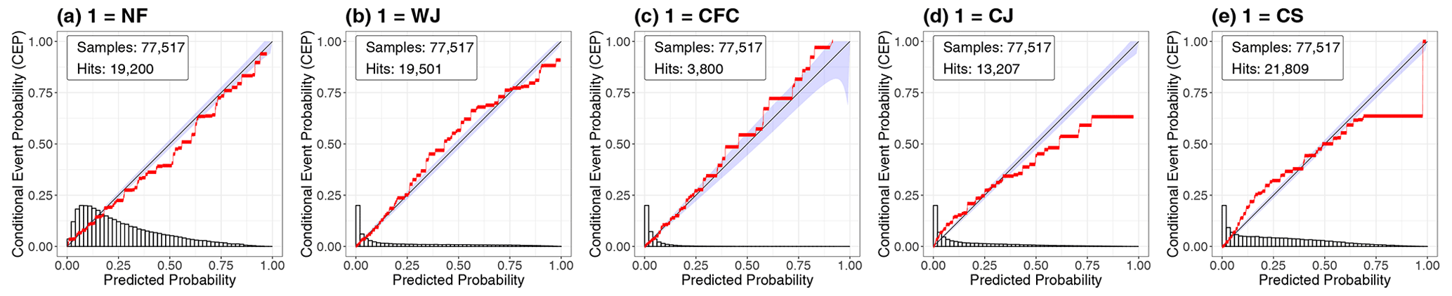
Figure 6 CORP reliability diagrams of the RF probabilities for the individual wind features in the one-against-all approach including all 12 storms.

The reliability diagrams of the all-pairs approach are displayed in Fig. 7 and show that the RFs yield well-calibrated probabilities for the distinction of all feature pairs except one. When the RF predicts that the CJ is more likely to occur than the CS (in case one of those two materialises), the RFs over-predict the CJ, meaning that the CS occurs more often than predicted (Fig. 7j). This is consistent with the results from the one-against-all approach, where we found that the CJ and CS predictions were not well calibrated for high probabilities, indicating that the RF fails to distinguish them for large conditional probabilities of the CJ. Further, the histogram of this pairwise comparison shows that the RF cannot discriminate between the two features with high confidence. This issue can be seen best for the storms Herwart and Sabine, which both did not develop a CJ, although a CJ was identified by the RFs (see Sect. 7.2). The main meteorological reason for this problem is the general similarity of the two features and that the hook-shaped structure, which is used for the subjective identification of a CJ, cannot be considered in the RF, such that the distinction is mainly based on p, as will be discussed in Sect. 6.2. Other than that, the calibration curves of the other pairs closely follow the diagonal. Moreover, we note that the WJ is distinguished well from the CJ and CS, as the U-shaped histograms of the probability distributions show (Fig. 7f, g).

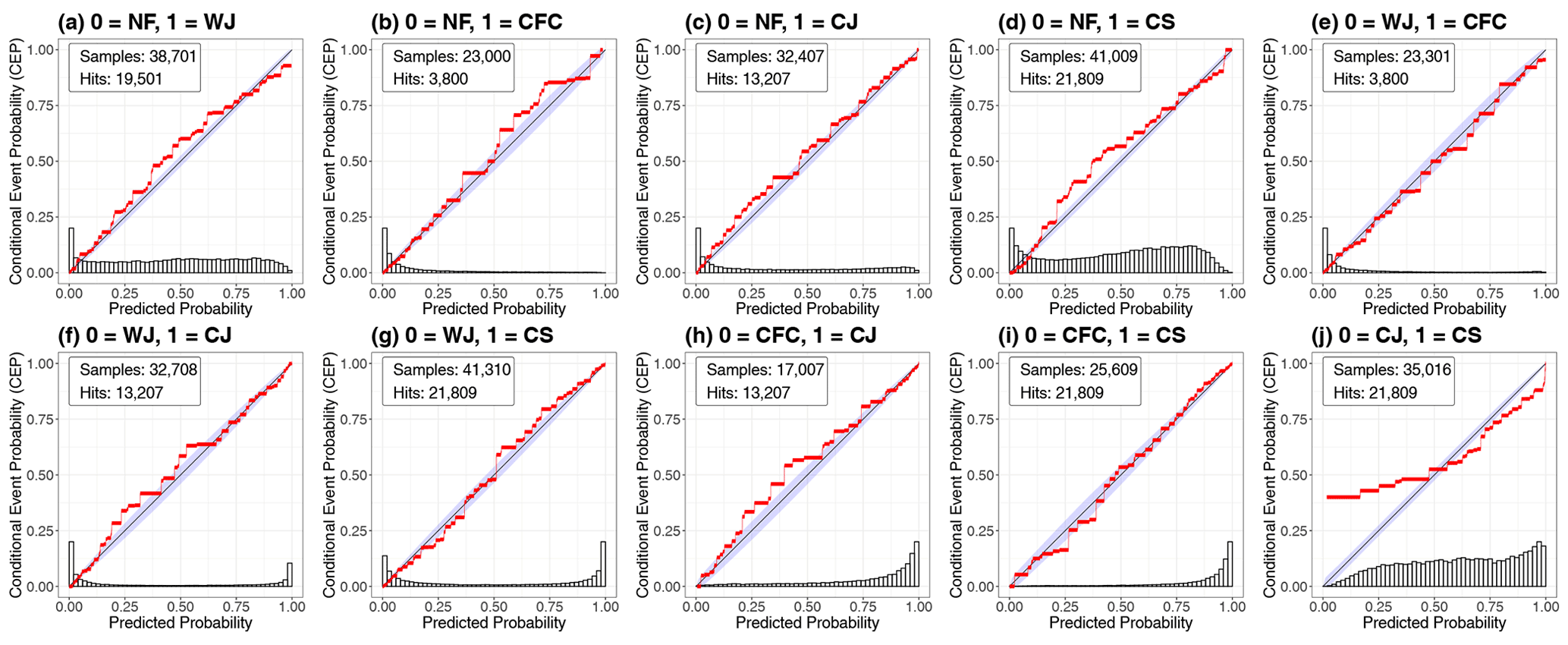
Figure 7 CORP reliability diagrams of the conditional RF probabilities comparing two wind features in the all-pairs approach including all 12 storms.

For the predictions derived from the COSMO-REA6 data, the RF probabilities are also able to distinguish the features well, although the RFs used were trained on station-based data. The predictions exhibit similar characteristics and perform (as expected) only slightly worse than for the station data. As before, the skill of the BS is calculated with respect to a benchmark prediction based on the class frequencies and is 19.6 % for all storms. For eight of the selected storms, we observe improvements ranging from 11.0 % to 37.5 %; however, for Herwart and Susanna, the skill scores are −0.8 % and −11.6 % respectively, indicating a decrease in predictive performance. For Susanna, this is due to a larger high-wind region ahead of but not directly connected to the cyclone for multiple time steps. While the predictions for Herwart look consistent in both data sets at first sight, fewer stations are available over Poland, where the CJ was over-predicted (see Sect. 7.2), such that the over-prediction in the gridded data carries more weight compared with the station data.

Further, at times, we find high probabilities of mostly the WJ in COSMO-REA6 in regions where winter storms are uncommon and where no features were labelled at all, e.g. in Italy and the Balkans (not shown). However, on the synoptic scale, the trough still affects some parameters in the region – that is, decreasing Δp on the eastern side of the core and d as the wind follows the isobars (not shown), which are the most important parameters to distinguish NF and the WJ (Fig. 9). Therefore, high winds caused by factors such as mountainous effects, including the foehn effect or land–sea breeze, might be falsely identified as a WJ. Thus, the RF should only be applied to regions affected by extratropical cyclones. As these regions have not been labelled (see Sect. 4.1), we excluded them from our evaluation.

The reliability diagrams of the one-against-all approach for the COSMO-REA6 data (see Fig. D2 in Appendix D) show that the calibration curves deviate more from the diagonal than for the station-based data (Fig. 6) but are still reasonably close to calibrated values. For the WJ and the CJ, we observe slight over-prediction (Fig. D2b, d), whereas we observe under-prediction for the CFC (Fig. D2c). For the CS, we observe a similar calibration curve to the station-based data (Fig. D2e). The distinction of the individual features, which we assess via the all-pairs approach in Fig. D3, results in mostly well-calibrated probabilities. The largest deviations from the calibration are observed again for the distinction of the CJ and the CS, as discussed above, and for the distinction of the WJ and the CFC (Fig. D3e), where the WJ is identified more frequently than observed. This might be caused by a spatially extended area of precipitation further into the warm sector at times due to missing data assimilation for that parameter (see Sect. 3.2). Overall, the predictions based on the COSMO-REA6 data are satisfactory considering that the RF models were trained on data from the station observations.

6.2 Predictor importance

To identify the predictors most relevant for the prediction of the wind features and the discrimination between two features, we calculate the BS permutation importance for the one-against-all and all-pairs approach. The BS permutation importance in the one-against-all approach is displayed in Fig. 8. In general, Δp is the most important predictor variable, especially for the WJ. Only for CFC is it not an important predictor, as it can occur slightly ahead of the cold-front-related pressure trough and, hence, in a region of positive Δp, as described in Sect. 2.4. On the other hand, the absolute values of p seem to be of less importance for the WJ and NF, which occur further away from the cyclone centre than the CJ and CS, for which p indicates the proximity to the cyclone centre. For CFC, we instead find that RR is the most relevant predictor variable (as expected), whereas it is less important for the WJ, CJ and CS. d seems to be relevant for most features, as it is a characteristic of the location relative to the cyclone centre. This also leads to a high importance for NF occurring more frequently north or west of the cyclone centre. However, d is not important for CFC, likely owing to the fact that convection leads to a more variable wind direction and due to the characteristic jump in d at cold fronts. On the contrary, Δd is of minor relevance for all features as well as $\mathrm{\Delta }\stackrel{\mathrm{̃}}{\mathit{\theta }}$. A more important temperature-based predictor seems to be $\stackrel{\mathrm{̃}}{\mathit{\theta }}$, although it is again less relevant for CFC. Lastly, $\stackrel{\mathrm{̃}}{v}$ shows its highest importance for NF, as higher wind speeds are less likely to be found at the boundary of a cyclone.

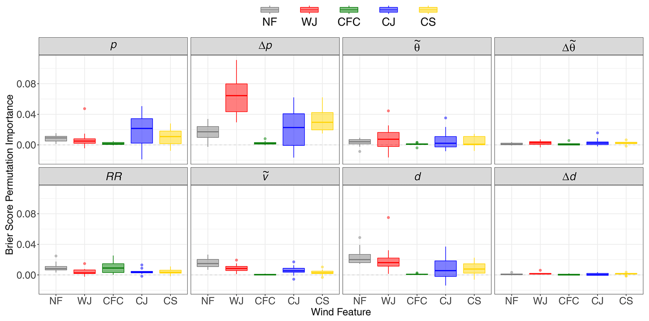
Figure 8 Boxplots of the BS permutation importance of the RF probabilities for the individual wind features and predictor variables in the one-against-all approach. The boxplots are calculated over the individual winter storms.

In the all-pairs approach (Fig. 9), we can attribute the importance of the predictor variables more accurately. The key to distinguish the WJ from all other features is Δp, especially from the CJ and CS. This is consistent with the one-against-all discussion above. The large outlier in Δp in the WJ vs. CJ is related to storm Herwart, as further discussed in the following section. Of secondary importance is d, particularly when compared to the CJ, CS and NF. Temperature also plays some smaller role in the distinction of the WJ. For CFC, the most important predictor by far is RR, but when compared against the CJ, p, Δp, $\stackrel{\mathrm{̃}}{\mathit{\theta }}$, $\mathrm{\Delta }\stackrel{\mathrm{̃}}{\mathit{\theta }}$ and d also contribute. The positive outlier in RR is related to storm Fabienne (not shown). The distinction of the CJ from other features is more complex. p is relevant in all CJ pairs, as already discussed. The distinction of CJ from NF additionally hinges upon Δp, $\stackrel{\mathrm{̃}}{\mathit{\theta }}$ and d.

The shortcomings of the RFs to distinguish CS and the CJ are also reflected in Fig. 9 by partly negative values of p, Δp and $\stackrel{\mathrm{̃}}{\mathit{\theta }}$. A negative value indicates that the RF probabilities perform better, when we break the link to the target variable by randomly permuting the predictor values. As discussed further in the following section, this is mostly due to storm Sabine, which reached an unusually low minimum core pressure of less than 950 hPa over the Norwegian Sea (see Fig. 2). Because of this, values of p in the CS over continental Europe were similar to values typical of a CJ.

Figure 9 Boxplots of the BS permutation importance of the RF probabilities comparing two wind features for the predictor variables in the all-pairs approach. The boxplots are calculated over the individual winter storms.

We do not only want to identify the most relevant predictors, we also want to investigate their effect on the predictions, which is illustrated for the eight predictor variables by the PDPs in Fig. 10. Again, the largest impact is found for Δp. The probability of observing a WJ is largest for small values of Δp and declines rapidly as the tendency increases and switches signs, while the probabilities of the CS and CJ increase. Probabilities of NF decrease slightly, while changes for CFC are small. For little RR, the probability of a CFC is close to zero, but it consistently increases with increasing precipitation. In turn, probabilities of other features slightly decrease with increasing precipitation. In general, the CJ and CS show high probabilities of low values of p, consistent with their occurrence during the most intense stage of a cyclone (see Sect. 2). However, surprisingly, CS shows higher probabilities than the CJ between 970 and 980 hPa, although the CJ is usually closer to the cyclone centre. This is again associated with the unusual behaviour of storm Sabine, with its deep pressure minimum but no subjectively identified CJ. As such intense cyclones are rare, we are confident that the RF performs well in most more ordinary cases. As discussed previously, d is dependent on the location relative to the cyclone centre. As the introduced features are all located south to west of the cyclone, we focus on values from 90 to 360^∘ only. Within the WJ, d values mostly show south-westerly winds and do not change drastically. Probabilities for CFC increase with a positive wind shift, leading to more westerly and north-westerly winds for CFC but also following features, i.e. the CJ and CS. Δd shows almost no change in probabilities for all features, consistent with its low BS permutation importance. $\stackrel{\mathrm{̃}}{\mathit{\theta }}$ shows an increasing trend for the WJ, while the probabilities decrease for the other features, most strongly for the CJ, as one would expect. For $\mathrm{\Delta }\stackrel{\mathrm{̃}}{\mathit{\theta }}$, we see indications of the air mass change at the cold front and, thus, higher probabilities in CFC for negative values. The CJ shows a slightly positive trend, whereas all of the others are flat.

Figure 10 Partial dependence plots for the predictor variables and wind features.

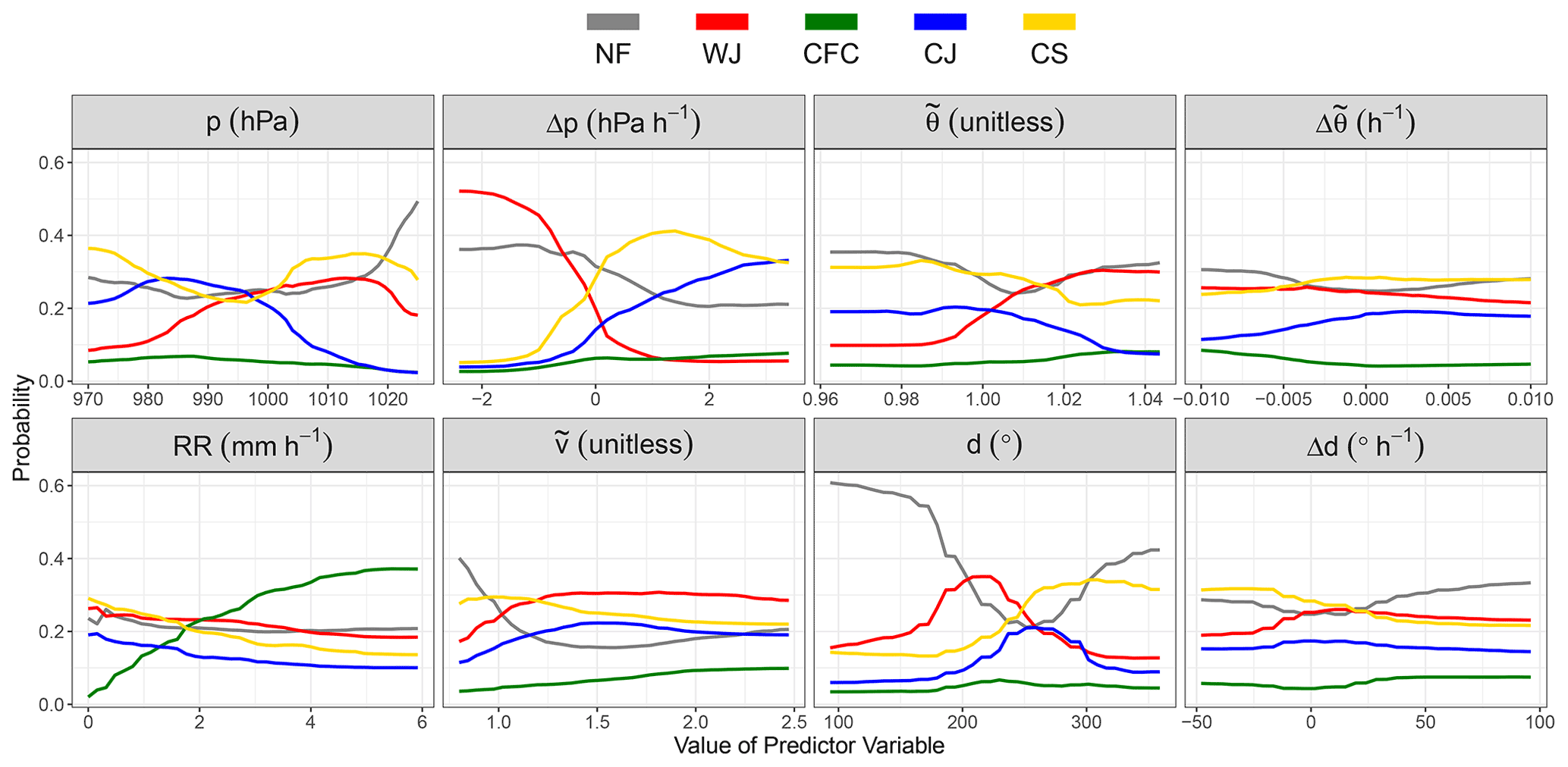
Overall, investigating the importance of the predictor variables for the predictions, we find that the RFs largely learn physically consistent relations, as described in Sects. 2 and 4.1.

7 Discussion

Section 5 showed a successful application of the introduced method to storm Burglind, both in station- and grid-based data sets. However, extratropical cyclones rarely follow the textbook NC model exactly. For example, sometimes high winds are mainly related to an exceptionally strong synoptic-scale pressure gradient rather than being associated with the mesoscale features that we have developed an objective identification algorithm for. As described in Sect. 4, we selected 12 windstorm case studies to train the RF based on surface observations with the diversity of cyclones and features in mind, such that the RF is representative for a climatology over a longer time period.

This section discusses how the trained RF deals with some well-known deviations from idealised cyclone models, such as double fronts and convergence lines (Sect. 7.1), large background pressure gradients (Sect. 7.2), and the specific characteristics of the SKC and SJ (Sect. 7.3). In addition, we further discuss the advantages and disadvantages of not using spatial dependencies in the feature identification (Sect. 7.4). A complete set of results for all case studies can be accessed in the Supplement (Eisenstein et al., 2022c).

7.1 Double fronts and convergence lines

Real-world frontal structures of extratropical cyclones can differ considerably from idealised conceptual models (e.g. in terms of complex vertical structure, strong tilts, or a secondary frontal zone parallel to the main front). Here, we are interested in synoptic systems with double cold fronts and convergence lines with high winds. While a cold front is associated with a second low-pressure trough, a convergence line develops where two airflows collide and can occur independently of a cyclone. The area between a primary and secondary cold front can have characteristics of a warm and/or cold sector; thus, high-wind features are predicted with higher uncertainty by the RF. This can also be the case for the area between a cold front and a convergence line.

The example from our selection of 12 cyclones that illustrates this best is Bennet. On 4 March 2019 at 12:00 UTC, the cyclone centre was located over the North Sea to the west of Denmark (Fig. 11a). The primary front was located at the north-eastern border of Germany and Bavaria and had already weakened (see Fig. D5 in Appendix D). A secondary strong temperature gradient could be found over north-western Germany, Luxembourg and France. However, it is uncertain, if this should be classified as a front or convergence line. While synoptic charts from the DWD show a convergence line, Met Office charts show an upper-level cold front at 06:00 UTC and an occluded front 6 h later. As this feature shows characteristics typical of CFC (see Sect. 2.4), it was ultimately labelled as such by the first author and is referred to as a secondary front.

Figure 11a shows the mesoscale wind features identified by the RF. At this time Bennet caused the highest winds slightly ahead of the secondary front and in a smaller region behind the primary front (see the dashed line in Fig. 11a). For the area between the fronts, the RF predicts both a CS and WJ with medium confidence. This is to be expected, as some parameters, especially Δp, $\stackrel{\mathrm{̃}}{\mathit{\theta }}$ and $\mathrm{\Delta }\stackrel{\mathrm{̃}}{\mathit{\theta }}$, show the behaviour of both features with a tendency towards a CS. RF predictions along the secondary front show only low probabilities of a CJ and CFC. However, at earlier and later time steps (i.e. ahead of the primary cold front and behind the secondary one), the prediction of the WJ, CJ and CS are accurate, as can be seen in the full animation provided in the Supplement (Eisenstein et al., 2022c). Thus, looking at the entire lifetime of the storm, satisfactory identification can be obtained from RAMEFI.

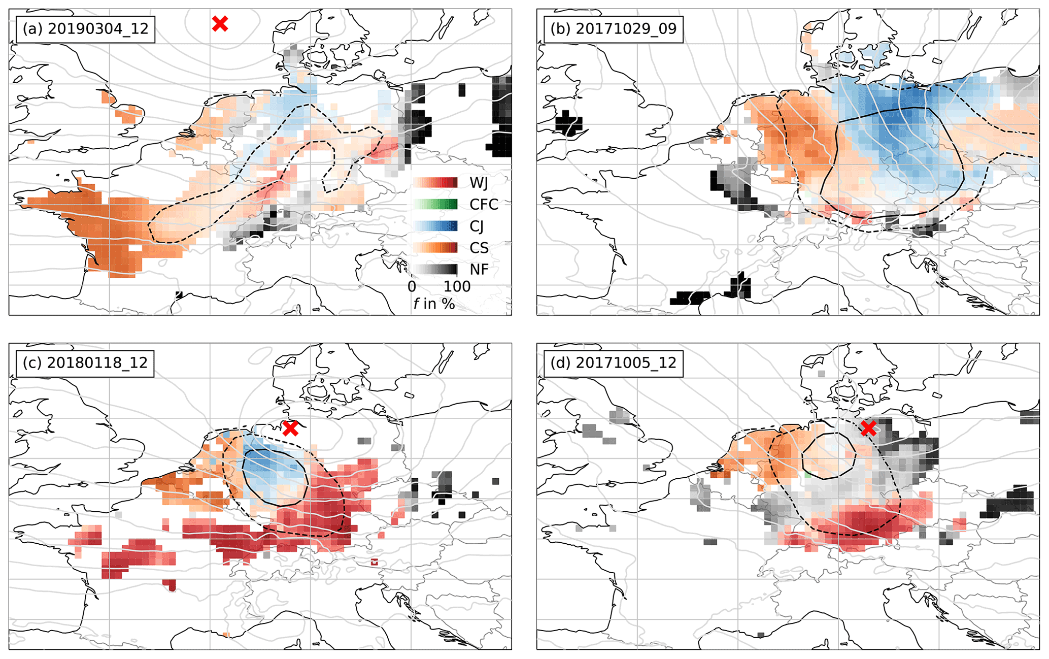
Figure 11 As in Fig. 4 but for (a) storm Bennet on 4 March 2019 at 12:00 UTC, (b) storm Herwart on 29 October 2017 at 09:00 UTC, (c) storm Friederike on 18 January 2018 at 12:00 UTC and (d) storm Xavier on 5 October 2017 at 12:00 UTC. Note that, at the time shown, storm Herwart had already exited the plot area to the east.

7.2 Strong background pressure gradients

Very intense cyclones are often accompanied by a strong large-scale pressure gradient (e.g. Fink et al., 2009), which, in turn, causes high wind speeds that are unconnected to one of the four mesoscale wind features under study but can be enhanced by them. With an underlying strong wind field, the detection and distinction of the features might be more complicated. Good examples from our list of case studies to illustrate this are the storms Herwart and Sabine. Figure 11b shows Herwart in a late development stage on 29 October 2017 at 09:00 UTC when the pressure gradient was already weakening (see the light grey contours). Around this time, the cyclone centre travelled over Poland (outside of the area shown in the figure). The occurrence of a CJ seems unlikely in that region, as a typical hook-shaped structure cannot be seen in wind observations (not shown). The occluded front was rather weak and did not fully wrap around the cyclone centre (see Fig. D6 in Appendix D). Therefore, ultimately, the already high wind speeds caused by a strong background pressure gradient over Germany (black lines in Fig. 11b) make the subjective labelling of additionally occurring features quite challenging. The RF shows high probabilities of a CJ for several hours in this region, although it was originally labelled to be CS. The main reason for this is that the proximity to the cyclone centre, reflected in the low value of p, is the most important predictor to distinguish the CJ and CS (Fig. 9). Nevertheless, even in this unusual case, the prediction by the RF is still reasonable, as both a subjective and objective identification of the two features here is ambiguous in surface observations alone.

In the case of Sabine, the cyclone centre did not cross continental Europe but moved through the Norwegian Sea (Fig. 2). The minimum pressure reached less than 950 hPa. Stations over central Europe still observed values of p below 970 hPa, which is lower than the cyclone centres of most of our other case studies, making Sabine a quite unusual case. As discussed in Sect. 6, this causes difficulties with respect to distinguishing the CJ and CS of Sabine, which is somewhat similar to Herwart. Although a CJ is identified in an area of low values of p, this region is not in the vicinity of the cyclone centre, as was the case for Herwart. An animation of the feature identification for all time steps of Sabine is provided in the Supplement (Eisenstein et al., 2022c). In this case the CJ–CS distinction issue could have been avoided to some extent by including spatial dependencies in the identification algorithm at the expense of losing the capability for flexible application, as discussed in Sect. 4. We will return to this issue in Sect. 7.4.

7.3 Shapiro–Keyser cyclones and sting jets

As already explained in Sect. 2, cold fronts of SKCs are usually weaker than those of NCs, such that CFC wind features hardly occur. A good example for this is storm Friederike. Figure 11c shows 12:00 UTC on 18 January 2018, when the cyclone centre just reached the North Sea coast of Germany. High probabilities of a WJ occur over central Germany, while a CJ is identified by the RF over north-eastern Germany. CFC probabilities are very low along the entire cold front. Lagrangian trajectories confirmed an SJ in the region where the CJ is identified during that time. As the CJ and SJ are considered together in this work (see Sect. 4.1), the area was labelled as CJ and, hence, identified accurately. This area also coincides with the highest wind speeds associated with Friederike (see the black lines in Fig. 11c). West of the identified CJ region, a CS feature is detected. This shows that a CJ and SJ indeed show similar characteristics in surface parameters and can be considered as one feature in this context.

7.4 Spatial independence

The decision not to use spatial (nor temporal beyond 1 h) dependencies in the identification algorithm makes our method highly flexible in its application, but the local approach can also cause issues where features deviate from their stereotypical characteristics. One example of the problem is the CJ of Sabine, as discussed in Sect. 7.2. Another example is storm Xavier, where many points within the vicinity of the cyclone show the highest probability of NF for several hours, rather than the probability of any of the mesoscale wind features (Fig. 11d). The main reason for this appears to be that Xavier was characterised by unusually cool $\stackrel{\mathrm{̃}}{\mathit{\theta }}$ and high p (not shown), generally two of the most important parameters to distinguish features (Fig. 8). While one predictor behaving in an unusual way could be compensated for, such as in the case of Fabienne (see  Eisenstein et al., 2022c), two anomalous behaviours unsurprisingly result in considerably greater uncertainty.

A possible solution to the issues described here on the basis of Sabine, Xavier and Fabienne is to not only regard anomalies from diurnal and seasonal cycles but also to include some kind of spatial background (e.g. by normalising p by the core pressure to detect the region close to the cyclone centre or by comparing $\stackrel{\mathrm{̃}}{\mathit{\theta }}$ to the mean state over Europe during the period of the storm to detect the warm sector). However, such a step would bring its own set of problems. Any spatial mean would require an arbitrary decision about the considered area, which may vary greatly from cyclone to cyclone. Moreover, spatial means computed from surface observations are not representative due to the irregular spacing of the stations. Essentially, as the features identified by the RF still occur in the expected areas, as described in Sect. 2, we conclude that a flexible local approach offers more advantages than disadvantages overall.

8 Conclusions

High wind and gust speeds can be caused by distinct mesoscale features within extratropical cyclones, which occur during different stages of the cyclone life cycle, in varying regions relative to the cyclone centre and have distinctive meteorological characteristics (e.g. Hewson and Neu, 2015). These differences likely imply differences in hazardousness, forecast errors and, hence, risk to life and property.

To better understand, monitor and predict these mesoscale features, we developed RAMEFI, a novel objective identification method that is able to reliably distinguish the four most important features: the WJ, the CJ, CFC and CS. The rare and often short-lived SJ is included in the CJ category, as the surface characteristics of these two features are often rather similar, and 3D trajectories are required for a clean distinction (Gray et al., 2021).

The first step was to build a browser-based, interactive tool to subjectively label surface stations over Europe for 12 selected winter storm cases between 2015 and 2020. Based on the outcome, we trained a probabilistic RF based on the following eight predictors: $\stackrel{\mathrm{̃}}{v}$, p, Δp, $\stackrel{\mathrm{̃}}{\mathit{\theta }}$, $\mathrm{\Delta }\stackrel{\mathrm{̃}}{\mathit{\theta }}$, RR, d and Δd. We note that we set a $\stackrel{\mathrm{̃}}{v}$ threshold of 0.8 to focus on high-wind areas. However, we do not expect the RF to be sensitive to small changes in the threshold, and, in principle, the RF can be applied to wind speeds below this level. Being independent of the spatial behaviour or gradients, the approach is very flexible and can be applied to single stations or grid points and various data sets with differing grid spacing. However, due to the fast movement of meteorological features in stormy situations, an hourly resolution is required, making the algorithm inapplicable to some climate data sets. To obtain areal information from irregular station data, Kriging was applied on the station-based probabilities generated by the RF.

The trained RFs are generally well calibrated. However, the distinction between a CJ and CS is more challenging, as the two features show similar characteristics in most parameters except for the fact that a lower value of p in the CJ is located nearer to the cyclone centre. Overall, the RFs learn physically consistent relations reflected in the importance of individual predictors. For example, while Δp appears to be most important for the WJ, CJ and CS, RR is substantial for the identification of CFC.

A detailed analysis of the RF feature probabilities for the selected cases shows a high consistency with the subjectively set labels with only a few disagreements, mostly in cases of large deviations from standard cyclone models. While the identification of WJs has the highest confidence, the identification of CFC is least certain due to relatively few surface stations reporting hourly precipitation and, thus, less training data. Even the distinction between the relatively similar CS and CJ works well in most cases and time steps. In some cases, however, high probabilities of CJs are predicted by the RF in areas where no CJ was subjectively identified due to a missing hook-shaped structure and occlusion front or owing to an overly large distance from the cyclone centre (e.g. Herwart and Sabine). Despite the spatial independence of the method, putting the predicted probabilities together on a horizontal map and following the storm evolution in time shows a high degree of coherence for each feature, demonstrating the success of our method.

The station-based RFs are also applied to COSMO reanalysis data without any adaptations to the new data set. Nevertheless, the obtained results are mostly consistent and only slightly less calibrated. This demonstrates that the method could be readily applicable to other analysis and forecast data sets. Although applying RAMEFI over regions other than that used in the training has not been examined yet, relying on location-independent predictors suggests that it should be possible with little or no modification.

Now that the RAMEFI method is fully developed, it enables a number of exciting follow-on studies (see Part 2 of this paper; Eisenstein et al., 2022d). In a next step, we plan to use the objective identification approach to compute a long-term climatology over Europe based on station observations and COSMO reanalysis data. Although, existing literature has discussed different causes of winds within extratropical cyclones, their climatologies have been based on more subjective categorisations for a limited sample size (e.g. Hewson and Neu, 2015; Earl et al., 2017). For the first time, RAMEFI will allow a statistically substantiated analysis of the characteristics of the mesoscale wind features in terms of size, lifetime, position relative to the cyclone core, occurrence relative to the life cycle of the cyclone and wind characteristics. Furthermore, a systematic forecast error analysis will reveal the extent to which forecast errors differ between the identified features and whether there are any significant, systematic deficits in their representation in models. Based on the outcome, we plan to subsequently work on a feature-dependent post-processing approach using the methods discussed in Schulz and Lerch (2022). This can ultimately improve the forecasts of strong winds and gust, thereby supporting the provision of better warnings with respect to top high wind gusts and timely forecasts of the associated impacts.

Appendix A: Storm severity index

The SSI was originally developed to estimate windstorm-related damage to buildings and infrastructure (Klawa and Ulbrich, 2003). With this aim, daily wind gust maxima (v_g,max) for DWD stations were first scaled by the 98th percentile (v_g,98,s) to take local conditions into account. Next, the exceedances above v_g,98,s are cubed to account for the wind destructiveness and are weighted by the population density as a proxy for the insurance values (damage covered by insurance). Later developments introduced formulations for grid-based data, i.e. reanalysis data and climate models, definition of affected areas (“windstorm footprints”), and feature tracking (e.g. Pinto et al., 2007; Leckebusch et al., 2008). Following Pantillon et al. (2018), we use the SSI formulation for station observations over Germany considering only the meteorological impact (no population weighting):

$$\begin{array}{}\text{(A1)}& \text{SSI}=\sum _{\text{station s}}{\left\{{\left({\displaystyle \frac{v_{\text{g,max,s}}}{v_{\text{g,98,s}}}}-\mathrm{1}\right)}^{\mathrm{3}}\right\}}_{v_{\text{g,max}}>v_{\text{g,98}}}.\end{array}$$

Daily maximum wind gusts over Germany are available from the DWD surface network (Deutscher Wetterdienst, 2022). The SSI is calculated for each single day and displayed in Table 2 for the 12 selected cases. If a storm affects the region for several days, the maximum SSI of the daily values is selected. As the aggregated SSI value is dependent on the number of stations, possible changes in the surface network need to be taken into account for when analysing longer time series. For the period of our case studies (2015–2020), the number of stations remained stable; thus, a comparison of the SSI values is largely fair. Still, the obtained SSI values only serve as a comparison for the selected case studies in this paper and should not be compared numerically to SSI values from other works.

Appendix B: Implementation details

In this section, we provide technical details on the evaluation of the RF probabilities, the probabilistic RFs and the Kriging.

B1 Evaluation of the RF probabilities

The CORP reliability diagrams were generated using the reliabilitydiag package (Dimitriadis et al., 2021), and the PDPs were generated using the pdp package (Greenwell, 2017). Each reliability diagram is based on the RF probabilities and observations of all storm cases. For the PDPs, one partial dependence curve has to be calculated for each RF generated in a fold of the cross-validation (i.e. for each winter storm). The final curves are then obtained by a weighted average depending on the sample size of the folds.

B2 Random forests

RF is implemented via the ranger package (Wright and Ziegler, 2017) in R (R Core Team, 2021). Table 1 summarises the predictors used, and Table B1 summarises the chosen tuning parameters. One question in the implementation is the handling of missing values, which an RF cannot process. The station-based samples frequently miss values of one or more predictor variables, especially precipitation is affected. We tried different strategies to handle missing values, such as leaving out instances with missing values or replacing the missing values with a mean value, and found similar results. Therefore, we decided to replace the missing values in order to use the largest sample size possible, which is desirable for the evaluation and the Kriging step. In each fold of the employed cross-validation scheme, the missing values (both in the training and test set) are replaced by the mean value of the associated predictor variable in the training set.

Table B1 Overview of the tuning parameters of the probabilistic RF.

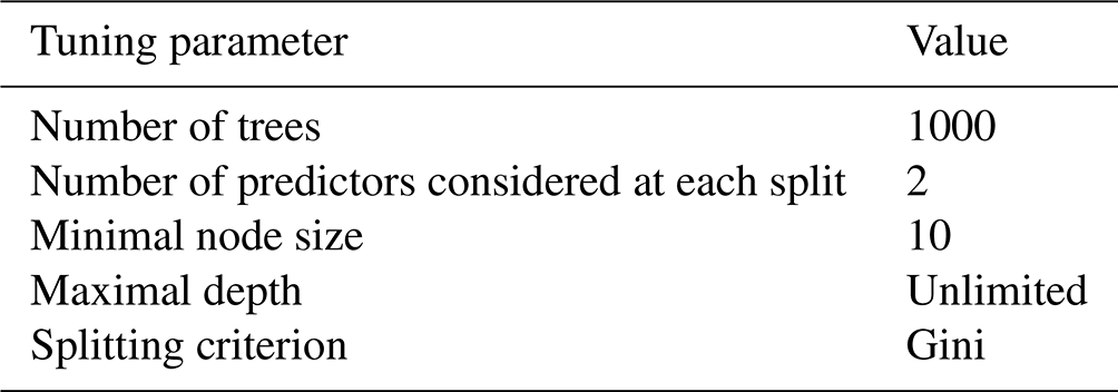
B3 Kriging

In our practical implementation of Kriging, we employ the fields (Nychka et al., 2017), mvtnorm (Genz et al., 2021), maps (Original S code by Richard A. Becker and Allan R. Wilks. R version by Ray Brownrigg. Enhancements by Thomas P Minka and Alex Deckmyn, 2018) and maptools (Bivand and Lewin-Koh, 2021) R packages. Additionally, we transform the probabilities by using the bestNormalize package (Peterson, 2021) to achieve approximate Gaussianity, which automatically chooses a suitable transformation from a set of commonly used transformations. The probabilities on the grid generated via the univariate Kriging need to be normalised such that they sum to one. However, at some grid cells distant from the cyclone track, the predicted probabilities are small for all of the wind feature and normalisation results in unrealistic predictions. Thus, we only perform the normalisation at grid cells where the accumulated probability is larger or equal to 20 %. For the visualisation, we further drop the grid cells where the largest normalised probability is smaller than 20 % (which includes the grid cells for which no normalisation was performed).

Appendix C: Mathematical details

In this section, we provide a more detailed description of the assessment of probability predictions and the Kriging approach.

C1 Assessing probability predictions of multiple classes

Consider a multi-class probability prediction $\mathit{f}=\left(f_{\mathrm{1}},\mathrm{\dots },f_k\right)$, where $f_{\mathrm{1}},\mathrm{\dots },f_k\in \left[\mathrm{0},\mathrm{1}\right]$ and ${\sum }_{i=\mathrm{1}}^k{f}_i=\mathrm{1}$, for a nominal target variable $Y\in \mathit{\{}\mathrm{1},\mathrm{\dots },k\mathit{\}}$ with k≥3 classes that are not ordered. In mathematical terms, f is called (auto-)calibrated if $\mathbb{P}\left(Y=i\mid \mathit{f}\right)=f_i$ for all $i=\mathrm{1},\mathrm{\dots },k$, where ℙ refers to the joint distribution of prediction and observation (Gneiting and Ranjan, 2013). The BS for a probability vector f and the realising class $i\in \mathit{\{}\mathrm{1},\mathrm{\dots },k\mathit{\}}$ is given by $S(\mathit{f},i)={\sum }_{j=\mathrm{1}}^k(f_j-\mathbb{1}\mathit{\{}i=j\mathit{\}}{)}^{\mathrm{2}}$, where 𝟙 denotes the indicator function (Brier, 1950). Now, consider a probability prediction $f\in \left[\mathrm{0},\mathrm{1}\right]$ for a dichotomous target variable $Y\in \mathit{\{}\mathrm{0},\mathrm{1}\mathit{\}}$. In mathematical terms, f is called calibrated if $\mathbb{P}\left(Y=\mathrm{1}\mid f\right)=f$ (Gneiting and Ranjan, 2013). The (binary) BS of a probability prediction f and realisation $y\in \mathit{\{}\mathrm{0},\mathrm{1}\mathit{\}}$ reduces to $S(f,y)=(f-y{)}^{\mathrm{2}}$. Both the binary and multivariate BS can be used to evaluate the improvement of a prediction method over a reference using the BSS. Given the mean BS of the predictions of interest ${\stackrel{\mathrm{‾}}{S}}_f$ and that of the reference predictions ${\stackrel{\mathrm{‾}}{S}}_{\mathrm{ref}}$, the skill score is calculated via ${\text{SS}}_f=\mathrm{1}-{\stackrel{\mathrm{‾}}{S}}_f/{\stackrel{\mathrm{‾}}{S}}_{\mathrm{ref}}$. Positive skill indicates improvement over the reference, with 100 % referring to a perfect prediction, 0 % referring to no improvement and a negative skill referring to a decrease in predictive performance with respect to the reference.

The one-against-all approach reduces the multi-class prediction problem to a set of k dichotomous problems. For each class $i\in \mathit{\{}\mathrm{1},\mathrm{\dots },k\mathit{\}}$, the probability f_i is a prediction for $\stackrel{\mathrm{̃}}{Y}=\mathbb{1}\mathit{\{}Y=i\mathit{\}}$, where 𝟙 denotes the indicator function. Note that evaluating the predictions f_i for $\stackrel{\mathrm{̃}}{Y}$ for each class is not equivalent to checking the multi-class calibration criterion, as the joint distribution of f_i and not that of f is considered in the one-against-all approach. The all-pairs approach reduces the multi-class prediction problem to a set of $k(k-\mathrm{1})/\mathrm{2}$ dichotomous problems. For each pair of classes (i,j), where $i,j\in \mathit{\{}\mathrm{1},\mathrm{\dots },k\mathit{\}}$ and i>j, we consider only samples with $Y\in \mathit{\{}i,j\mathit{\}}$. Then, the conditional probability ${\stackrel{\mathrm{̃}}{f}}_{i,j}$ is a prediction for $\stackrel{\mathrm{̃}}{Y}$, where

$${\stackrel{\mathrm{̃}}{f}}_{i,j}={\displaystyle \frac{f_i}{f_i+f_j}}\text{and}\stackrel{\mathrm{̃}}{Y}=\left\{\begin{array}{ccc}\mathrm{1}& \text{for}& Y=i,\\ \mathrm{0}& \text{for}& Y=j.\end{array}\right.$$

C2 Kriging

Let $\mathit{\left\{}X\right(\mathit{s}),\mathit{s}\in {\mathbb{R}}^{\mathrm{2}}\mathit{\}}$ be the spatial Gaussian process modelling the transformed probability of a certain wind feature, indexed by the spatial coordinates s that correspond to the latitude and longitude associated with the (transformed) probability. Further, we denote the mean function by 𝔼{X(s)}=μ(s) and the covariance function by $\text{Cov}\mathit{\left\{}X\right(\mathit{s}),X({\mathit{s}}^{\prime }\left)\mathit{\right\}}=C(\mathit{s},{\mathit{s}}^{\prime })$. Then, for a given set of station-based data $\mathit{x}=\mathit{\left\{}X\right({\mathit{s}}_{\mathrm{1}}),\mathrm{\dots },X({\mathit{s}}_n){\mathit{\}}}^T$, the spatial prediction at a grid cell s₀ is given as $\widehat{X}\left({\mathit{s}}_{\mathrm{0}}\right)=\mathit{\mu }\left({\mathit{s}}_{\mathrm{0}}\right)+{\mathbf{\Sigma }}_{\mathrm{12}}{\mathbf{\Sigma }}_{\mathrm{22}}^{-\mathrm{1}}(\mathit{x}-\mathit{\mu }),$ where $\mathit{\mu }=\mathit{\left\{}\mathit{\mu }\right({\mathit{s}}_{\mathrm{1}}),\mathrm{\dots },\mathit{\mu }({\mathit{s}}_n){\mathit{\}}}^T$, ${\mathbf{\Sigma }}_{\mathrm{12}}=\mathit{\left\{}C\right({\mathit{s}}_{\mathrm{0}},{\mathit{s}}_{\mathrm{1}}),\mathrm{\dots },C({\mathit{s}}_{\mathrm{0}},{\mathit{s}}_n\left)\mathit{\right\}}$ and ${\mathbf{\Sigma }}_{\mathrm{22}}=\mathit{\left\{}C\right({\mathit{s}}_i,{\mathit{s}}_j){\mathit{\}}}_{i,j=\mathrm{1}}^n$. Additionally, one can obtain the prediction variance as $\text{Var}\mathit{\left\{}\widehat{X}\right({\mathit{s}}_{\mathrm{0}}\left)\mathit{\right\}}=C({\mathit{s}}_{\mathrm{0}},{\mathit{s}}_{\mathrm{0}})-{\mathbf{\Sigma }}_{\mathrm{12}}{\mathbf{\Sigma }}_{\mathrm{22}}^{-\mathrm{1}}{\mathbf{\Sigma }}_{\mathrm{12}}^T$, and the full predictive distribution is obtained as $X\left({\mathit{s}}_{\mathrm{0}}\right)\mid \mathit{x}\sim \mathcal{N}\left(\widehat{X}\right({\mathit{s}}_{\mathrm{0}}),\sqrt{\text{Var}\mathit{\left\{}\widehat{X}\right({\mathit{s}}_{\mathrm{0}}\left)\mathit{\right\}}})$.

The choice and estimation of the mean function μ(⋅) and the covariance function $C(\cdot ,\cdot )$ are key elements of the Kriging implementation. While one can choose any parametric or nonparametric functional representation for μ(⋅), the valid choice for $C(\cdot ,\cdot )$ is limited to the class of positive semi-definite functions. In practice, the covariance function is often assumed to be stationary, which implies that the covariance function depends on the spatial locations only through spatial lags, i.e. $C({\mathit{s}}_i,{\mathit{s}}_j)=K({\mathit{s}}_i-{\mathit{s}}_j)$ for some positive semi-definite function K(⋅). In our implementation, we have specified the mean function $\mathit{\mu }(\cdot )=c,c\in \mathbb{R}$ to be a function with a constant value and the covariance function K(⋅) to be the Matérn class of stationary covariance function (Matérn, 1986).

Appendix D: Further figures

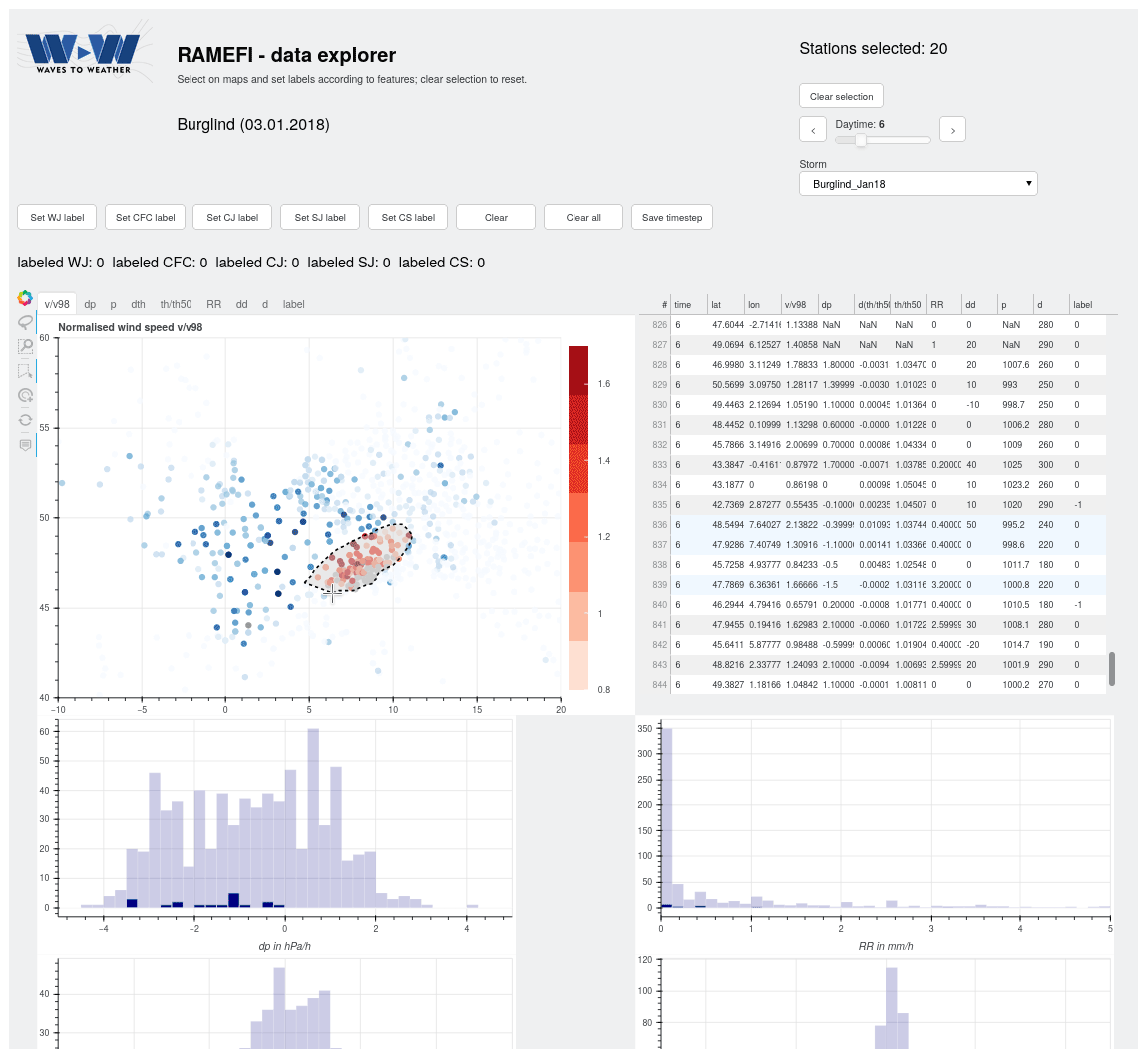
Figure D1 Screenshot of the interactive visualisation and labelling tool as part of RAMEFI (Eisenstein et al., 2022a) using the Bokeh (Bokeh Development Team, 2021) Python package. The user can switch between time steps and loaded winter storms. The top row shows a map of stations and their parameters, here $\stackrel{\mathrm{̃}}{v}$, where the user can select an area by mouse with the lasso tool or by clicking on single stations. Labels for the introduced features can be set for the selected stations. A table includes all data points and parameters. Histograms are shown for several parameters for the whole region (light blue) and for currently selected stations (dark blue).

Figure D2 As in Fig. 6 but based on COSMO-REA6 data.

Figure D3 As in Fig. 7 but based on COSMO-REA6 data.

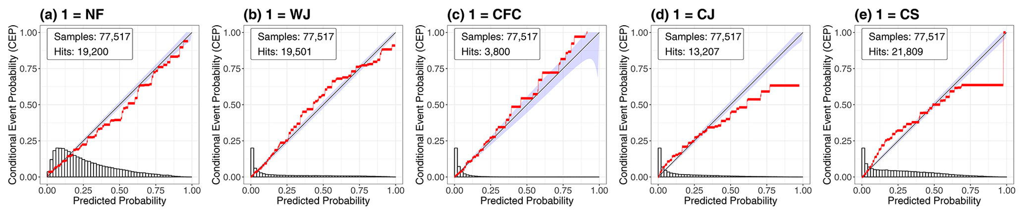
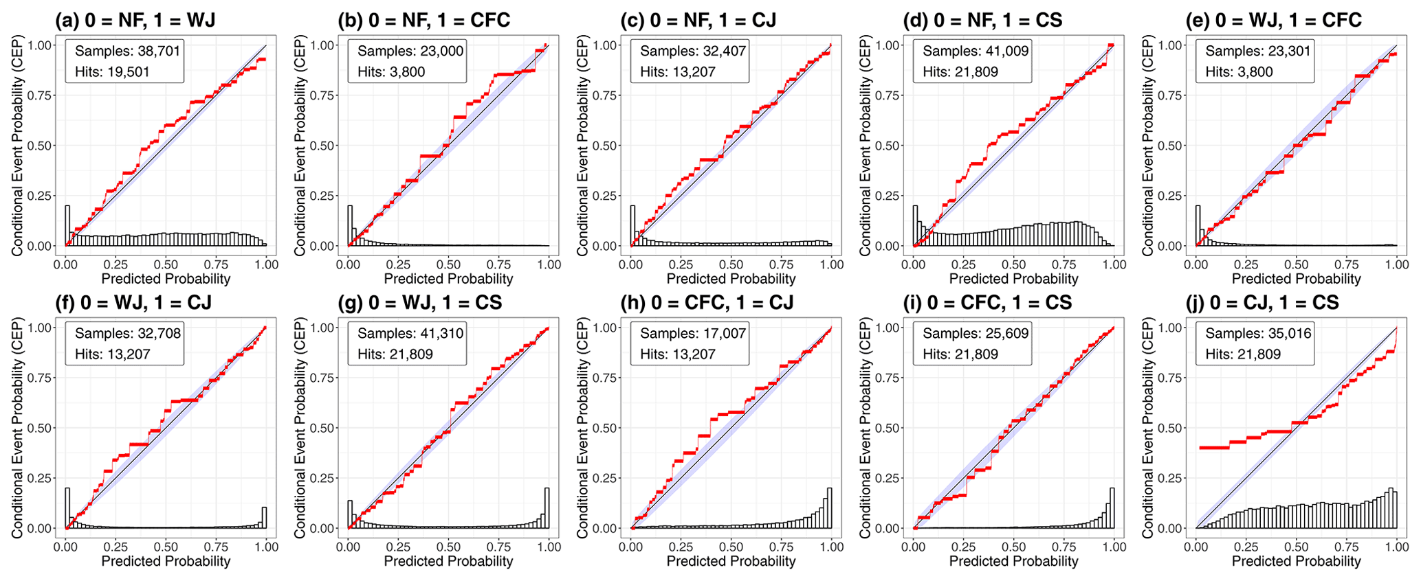
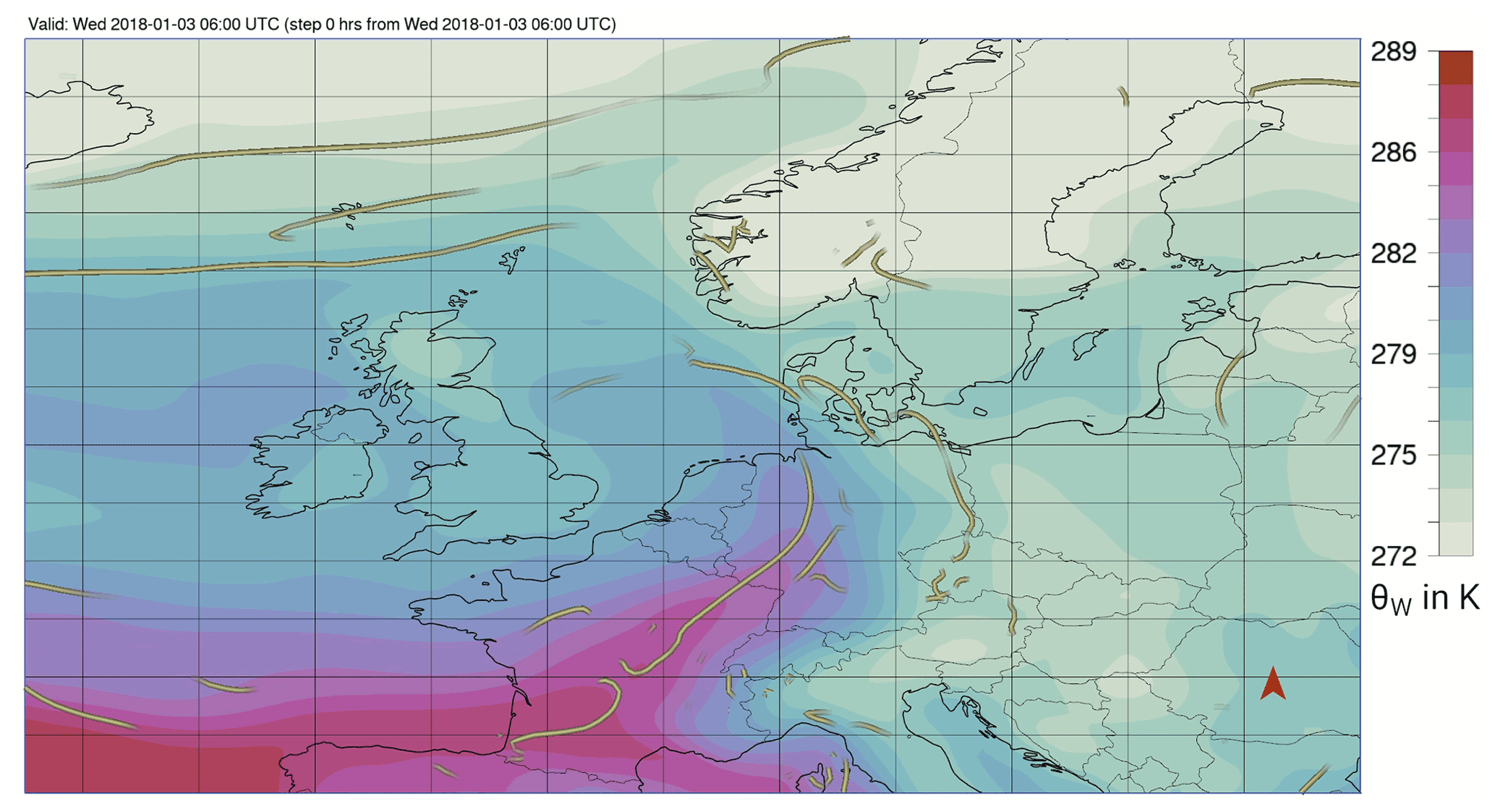
Figure D4 Detected fronts at 850 hPa (green tubes) and wet-bulb potential temperature θ_W (shading) for storm Burglind on 3 January 2018 at 06:00 UTC using the Met.3D visualisation software (Beckert et al., 2022; Rautenhaus et al., 2015). Data source: ERA5.

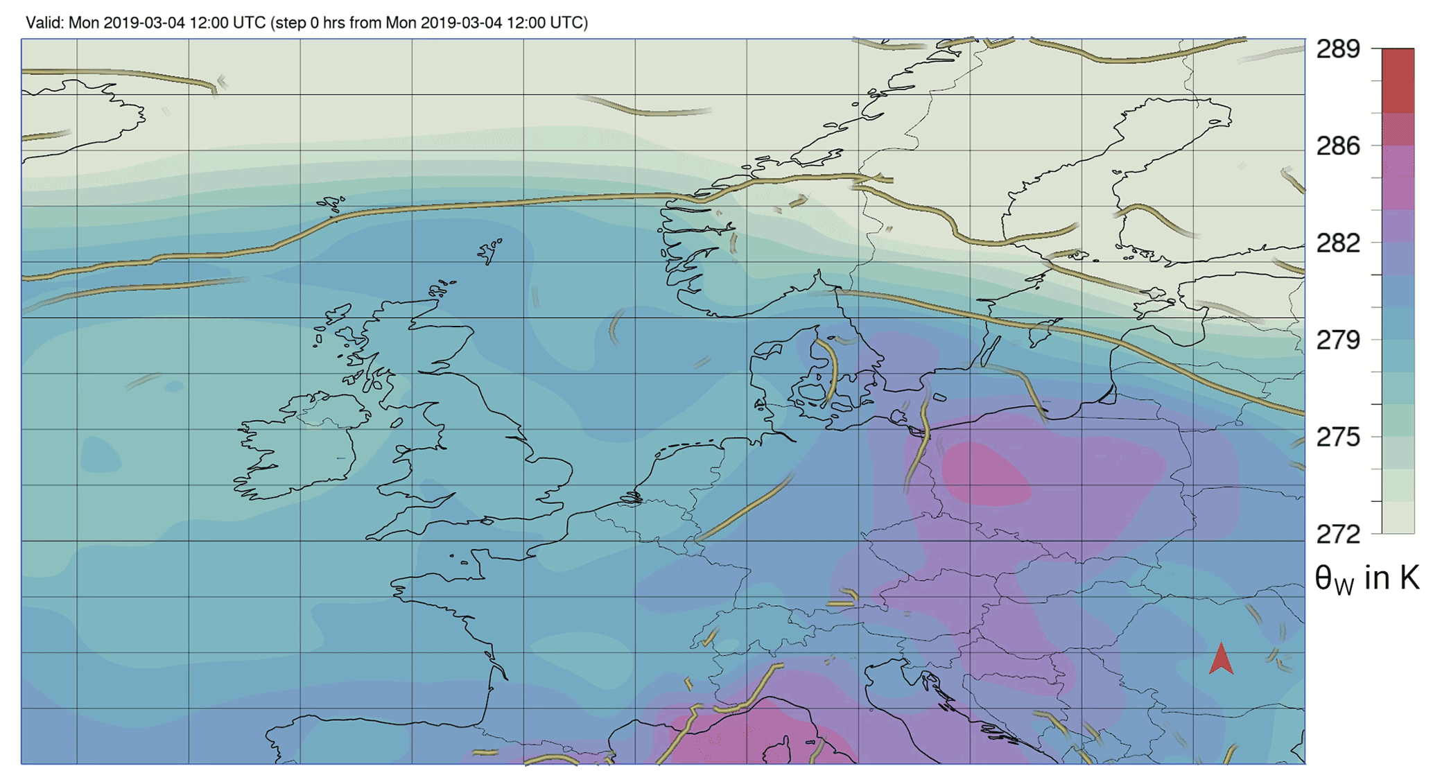
Figure D5 As in Fig. D4 but for storm Bennet on 4 March 2019 at 12:00 UTC.

Figure D6 As in Fig. D4 but for storm Herwart on 29 October 2017 at 09:00 UTC.