Stratospheric intrusion depth and its effect on surface cyclogenetic forcing: an idealized potential vorticity (PV) inversion experiment

Stratospheric intrusions of high potential vorticity (PV) air are well-known drivers of cyclonic development throughout the troposphere. PV anomalies have been well studied with respect to their effect on surface cyclogenesis. A gap however exists in the scientific literature describing the effect that stratospheric intrusion depth has on surface cyclogenetic forcing. Numerical experiments using PV inversion diagnostics reveal that stratospheric depth is crucial in the intensity of cyclonic circulation induced at the surface. In an idealized setting, shallow, high-PV intrusions (above 300 hPa) resulted in a marginal effect on the surface, whilst growing stratospheric depth resulted in enhanced surface pressure anomalies and surface cyclonic circulation. It is shown that the height above the surface that intrusions reach is more critical than the vertical size of the intrusion when inducing cyclonic flow at the surface. This factor is however constrained by the height of the dynamical tropopause above the surface. The width of the stratospheric intrusion is an additional factor, with broader intrusions resulting in enhanced surface cyclogenetic forcing.

1 Introduction

Potential vorticity (PV) has been well established as a highly useful and important parameter within dynamical meteorology (Hoskins et al., 1985). The usefulness of a PV framework for both operational and academic meteorological analyses is primarily drawn from two characteristics of PV. The first is the fact that PV is conserved for adiabatic and frictionless flow (Hoskins et al., 1985; Holton and Hakim, 2013). The second of these characteristics is the invertibility of PV (e.g. Røsting and Kristjánsson, 2012). PV inversion, under suitable balance and boundary conditions, allows for the calculation of other meteorological parameters such as pressure and wind velocity as a result of a distribution of PV (Lackmann, 2011; Davis, 1992b). Kleinschmidt (1950) introduced the initial ideas of PV invertibility for specific cases, attributing circulation patterns in the low levels to an upper-level PV anomaly and introducing the idea of deducing wind, pressure and temperature fields from PV distributions. PV invertibility became more refined and generalized through the development of quasi-geostrophic theory (Charney and Stern, 1962) and is still continually being developed and improved on today. PV frameworks and invertibility however only started to be a staple of dynamical meteorological analyses after the landmark paper by Hoskins et al. (1985).

PV invertibility has allowed for the study of different meteorological phenomena such as cyclogenesis from a PV perspective (e.g. Davis and Emanuel, 1991). A key principle in PV analyses is the definition of the dynamical tropopause. Traditionally, the tropopause separates the stratosphere, which is highly stratified, from the troposphere (Kunz et al., 2011). The strict definition from a dynamical or PV perspective is based on the gradient of isentropic PV contours (Reed, 1955). However, for simplicity, a PV iso-surface is often used. The exact value of PV often differs; however, −1.5 and −2.0 PVU (1 PVU = 10⁶ K m² s⁻¹ kg⁻¹) contours (in the Southern Hemisphere) are the most common (e.g. Lackmann, 2011). The identification of the dynamical tropopause is crucial in PV analyses. Tropospheric folds can reveal upper-tropospheric fronts and upper-level PV anomalies (Sprenger et al., 2003). Rossby wave breaking (RWB) is often associated with the isentropic transport of high-PV (large negative values in the Southern Hemisphere) anomalies of stratospheric air into the troposphere (e.g. Thorncroft et al., 1993; Ndarana and Waugh, 2011; Barnes et al., 2021a). PV inversion shows that these high-PV (large negative) anomalies result in cyclonic flow around the anomaly and cyclogenesis. Theories of high-PV anomalies have been discussed by various authors and basic meteorological texts (Hoskins et al., 1985; Holton and Hakim, 2013; Lackmann, 2011) and have led to the basic conceptual model for cyclonic PV anomalies as shown in Fig. 1. The conceptual model clearly shows the vast cyclonic motion around the upper-level PV anomaly. This also extends to the surface beneath the upper-level anomaly.

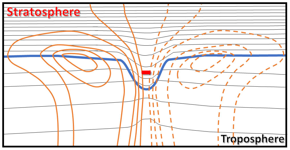
Figure 1 Conceptual model of a cross-section through a high-PV anomaly (negative sign in red) in the Southern Hemisphere (adapted from Lackmann, 2011). Black lines represent isentropes, whilst orange lines represent meridional wind velocities (dotted negative, solid positive). The bold blue line represents the dynamical tropopause (a constant PV contour).

Several studies have shown cases of cyclogenesis and their development in the presence of stratospheric intrusions of high PV (e.g. Davis and Emanuel, 1991; Davis, 1992a; Iwabe and Da Rocha, 2009; Barnes et al., 2021b). Bierly (1997) confirmed this link through composite analysis and showed the importance of the upper-level intrusion during cyclones' initial development. Many studies have focussed on rapid cyclogenesis. A landmark case study shows a tropopause fold that developed in relation to the President's Day cyclone over the east coast of the United States (Uccellini et al., 1985). Rapid cyclogenesis has since been linked to the presence of a PV tower – an alignment of three distinct PV anomalies, in the upper troposphere, lower troposphere and surface (e.g. Čampa and Wernli, 2012). PV inversion is the perfect tool to infer how various PV anomalies affect cyclogenetic forcing throughout the troposphere and stratosphere and has been used extensively throughout the scientific literature for this purpose. For example, extratropical cyclogenesis has been studied in the context of how different PV anomalies throughout the troposphere interact to influence cyclogenesis (Huo et al., 1999). Through the analysis of case studies, it was shown that the vertical alignment and phase of PV anomalies throughout the troposphere, together with interactions between the main upper-level anomaly and smaller anomalies within the upper-level mean flow, are important to cyclogenesis. PV inversion has also been used to show the effect of upper-level anomalies in a variety of other extra-tropical (Ahmadi-Givi et al., 2004; Pang and Fu, 2017) and tropical (Arakane and Hsu, 2020; Moller and Montgomery, 2000) settings. Other studies have used PV inversion to diagnose numerical weather prediction (NWP) errors (Brennan and Lackmann, 2005) and the effect on downstream precipitation (Baxter et al., 2011). Few studies have used PV inversion in an idealized setting to study the upper-level and stratospheric intrusion depth's influence on cyclogenesis, especially from a southern hemispheric point of view. A study of stratospheric depths in relation to surface cyclogenesis was performed in relation to cut-off lows (COLs) by Barnes et al. (2021a). This study was done from a climatological point of view in the Southern Hemisphere. The results show that stratospheric intrusions with a −1.5 PVU tropopause associated with COLs detected on the 250 hPa pressure level that extend to 300 hPa or below are more likely to result in surface cyclogenesis. The COL extension climatology by Barnes et al. (2021a) was based on real-case reanalysis data. As reanalysis data, climatological averages and composites were used; the isolated effect that the PV intrusions studied by Barnes et al. (2021a) had on surface cyclogenesis was not considered. Studying these processes in an idealized setting will add to our understanding of the effect that stratospheric intrusions have on surface processes.

In this study, the effect that the stratospheric intrusion depth has on surface cyclogenetic forcing is studied in an idealized setting. Although the effect that stratospheric intrusions have on surface cyclogenesis is not a new concept (e.g. Hoskins et al., 1985), this study examines the effect that stratospheric depth and intrusion characteristics have on surface cyclogenetic forcing in a systematic way. The systematic methodology utilized allows for a correlation between intrusion depths, widths and intensities with the intensity of cyclogenetic forcing at the surface. Although analytical-type analyses are possible in order to attempt to solve some of the issues addressed in this work, numerical experimentation is chosen due to the complexity of the analyses. The idealized numerical experimentation of PV intrusions aims to enhance our understanding of the effect PV intrusion depth has on surface cyclogenetic forcing as described in basic theoretical texts (e.g. Hoskins et al., 1985) and corroborate the findings and hypothesis of the climatology by Barnes et al. (2021a), which is that deeper intrusions are responsible for deeper COLs and surface cyclone development. A collection of numerical experiments using the power of PV inversion is used. Various experiments using variations in the depth and intensity of the simulated intrusion, as well as variations in the dynamical tropopause height, are performed. This paper is organized as follows. Section 2 introduces the piecewise PV inversion algorithms used for the experiment, as well as the various experimental setups for each test. The results of these tests are presented in Sect. 3. The results are finally discussed holistically, and conclusions are drawn in Sect. 4.

2 Methodology

2.1 Piecewise PV inversion algorithm

PV invertibility is a mathematical construct. The basic mathematical ideas have been fully described in many textbooks. From Holton and Hakim (2013), quasi-geostrophic PV (q) can be expressed mathematically by

$$\begin{array}{}\text{(1)}& q={\mathit{\zeta }}_{\mathrm{g}}+f+f{\displaystyle \frac{\partial }{\partial z}}\left({{\displaystyle \frac{\partial \stackrel{\mathrm{‾}}{\mathit{\theta }}}{\partial z}}}^{-\mathrm{1}}\mathit{\theta }\right),\end{array}$$

with ζ_g the geostrophic relative vorticity, f the Coriolis parameter (f<0 in the Southern Hemisphere), θ the potential temperature and $\stackrel{\mathrm{‾}}{\mathit{\theta }}$ the potential temperature of the reference state. The aim of the invertibility principle is to return a variable, say pressure p, by inverting Eq. (1).

In this study, numerical experiments are performed utilizing the PV inversion framework of Fehlmann (1997). The set of code is designed for reanalysis datasets to diagnose the effect that PV anomalies have on the surrounding meteorological parameters. In this study, however, we use an extension of these algorithms which allows for more idealized experimentation (Fehlmann, 1997; Sprenger, 2007). The set of numerical codes solve the Neumann boundary problem for potential vorticity q and the streamfunction ψ from which the wind components can be derived, given by the quasi-geostrophic PV:

$$\begin{array}{}\text{(2)}& q={\displaystyle \frac{{\partial }^{\mathrm{2}}\mathit{\psi }}{\partial x^{\mathrm{2}}}}+{\displaystyle \frac{{\partial }^{\mathrm{2}}\mathit{\psi }}{\partial y^{\mathrm{2}}}}+{\displaystyle \frac{f^{\mathrm{2}}}{\stackrel{\mathrm{‾}}{\mathit{\rho }}}}{\displaystyle \frac{\partial }{\partial z}}\left({\displaystyle \frac{\stackrel{\mathrm{‾}}{\mathit{\rho }}}{{\stackrel{\mathrm{‾}}{N}}^{\mathrm{2}}}}\cdot {\displaystyle \frac{\partial \mathit{\psi }}{\partial z}}\right),\end{array}$$

where $\stackrel{\mathrm{‾}}{\mathit{\rho }}$ and $\stackrel{\mathrm{‾}}{N}$ denote the density and Brunt–Väsälä for the reference state respectively. The boundary values of potential temperature at the lower and upper boundaries are given by

$$\begin{array}{}\text{(3)}& g\cdot {\displaystyle \frac{{\mathit{\theta }}^{\ast }}{\stackrel{\mathrm{‾}}{\mathit{\theta }}}}=f\cdot {\displaystyle \frac{\partial \mathit{\psi }}{\partial z}},\end{array}$$

whilst the lateral boundary condition for the u and v wind components are given by

$$\begin{array}{}\text{(4)}& u=-{\displaystyle \frac{\partial \mathit{\psi }}{\partial y}};v={\displaystyle \frac{\partial \mathit{\psi }}{\partial x}}.\end{array}$$

Using various partial differential equations and discretization techniques as shown in detail by Sprenger (2007) and Fehlmann (1997), the above problem can be solved numerically. For details about the numerical aspects of the PV inversion framework, based on successive over-relaxations, see Fehlmann (1997) and Sprenger (2007).

The idealized setup tool of Fehlmann (1997) allows the user to create an idealized basic state. This basic state is based on a user-defined jet stream (height, width, depth and intensity), dynamical tropopause height, static stability (of both the troposphere and stratosphere), latitude and surface baroclinicity. Potential temperature profiles are constructed from the available input by so-called “kink” functions (Fehlmann, 1997). Once defined and set up, a PV anomaly can be defined and introduced into the basic state. The code allows the user to define the intensity of the anomaly, vertical and horizontal dimensions, and positions.

2.2 Experimental setup

The idealized numerical experimental domain in this study has a zonal dimension of 7500 km and a meridional dimension of 5000 km with a 25 km horizontal resolution. In the vertical, 200 levels are specified with the upper limit at 20 000 m above ground level (a.g.l.) and the lower limit on the surface. The vertical levels have a resolution of 100 m. The PV inversion algorithm allows the user to specify the surrounding environment for the experiment. In this study, we aim to replicate the conditions of the climatology presented by Barnes et al. (2021a), where the dynamical tropopause is considered to be the −1.5 PVU iso-surface. The PV inversion algorithm however requires a dynamical tropopause height a.g.l. which corresponds to the −2 PVU contour. To comply with the convention of the code, the dynamical tropopause is set at a specific height value a.g.l. The height of the −1.5 PVU iso-surface (which is the defined dynamical tropopause used in this study) is calculated from the field after the simulation. The static stability parameters are then set by specifying Brunt–Väisälä frequencies of 0.01 and 0.03 s⁻¹ for the troposphere and stratosphere respectively such that the −1.5 PVU iso-surface can be considered the clear divide between the stratosphere and the troposphere. This is shown by the meridional PV cross-section of the basic state in Fig. 2. In this field, the dynamical tropopause was set to 12 500 m a.g.l., whilst the resulting −1.5 PVU contour (effective dynamical tropopause) was calculated to be at 11 285 m a.g.l.

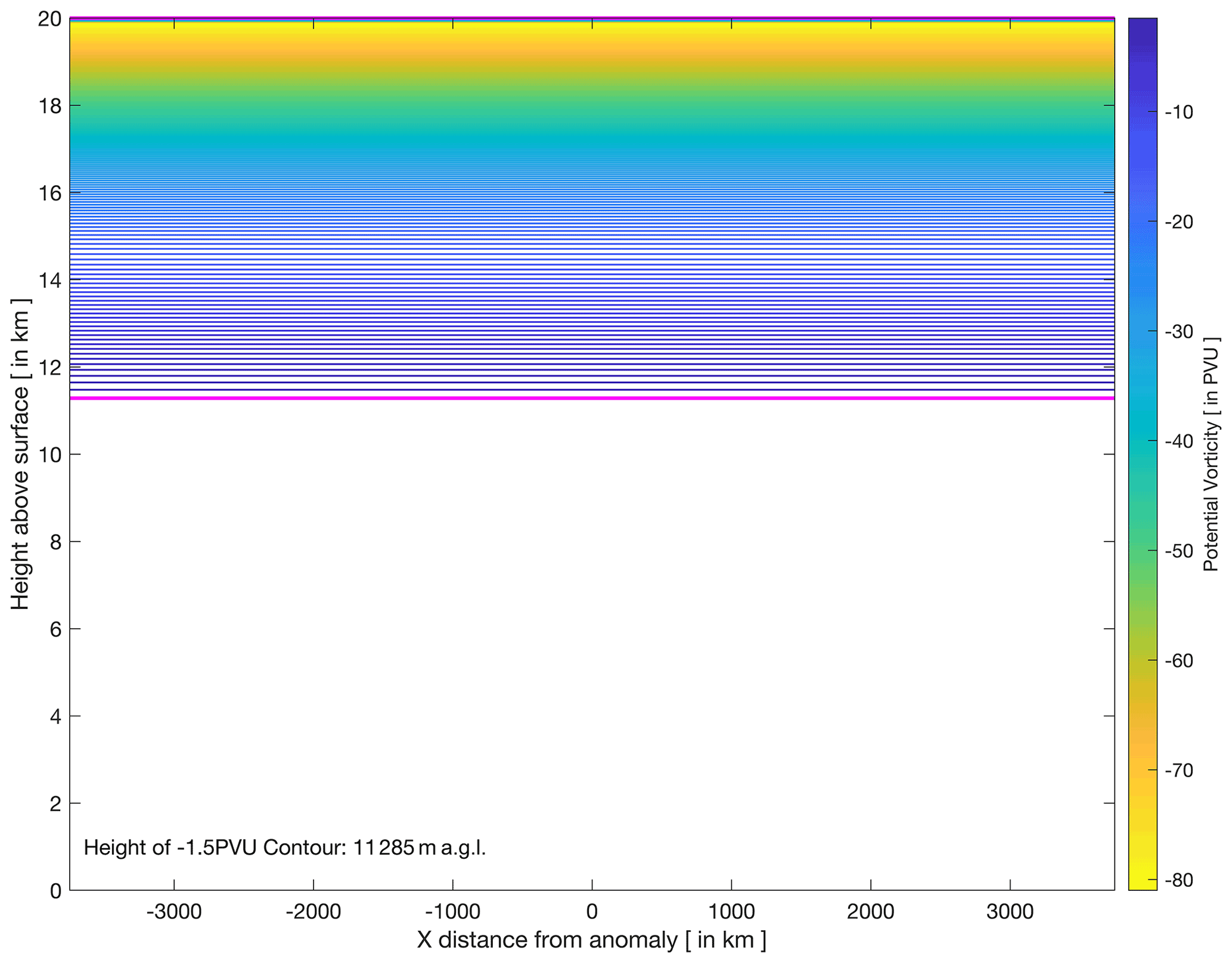
Figure 2 PV zonal cross-section through the centre of the domain. The −2 PVU tropopause was specified at a height of 12 500  m a.g.l. The −1.5 PVU contour (highlighted by a thick magenta line) was calculated to be 11 285 m a.g.l. A contour interval of 0.5 PVU is used.

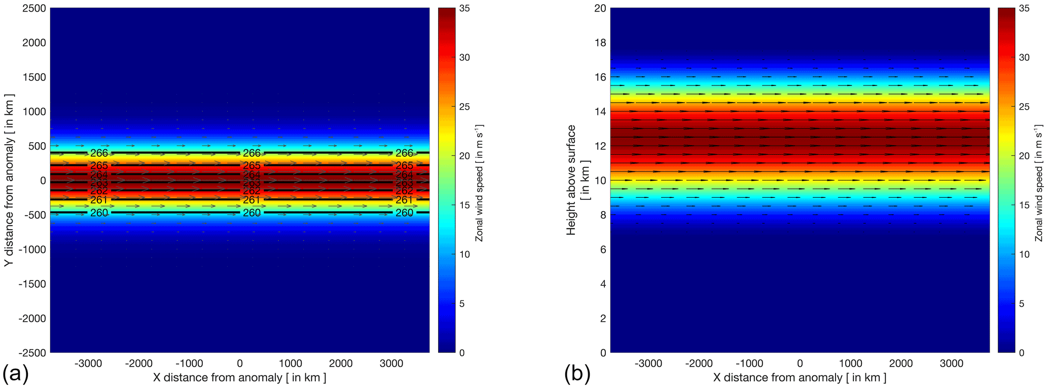
Figure 3 The jet stream of the model setup. (a) The zonal wind speed of the jet stream at the height of the given model's tropopause (12 500 m a.g.l.). Pressure contours (in hPa) are overlaid together with zonal wind quivers. (b) A cross-sectional view of the zonal wind associated with the jet stream through the centre of the domain overlaid with zonal wind quivers.

The algorithm also allows for the specification of the jet stream in the upper levels. The jet was centred around the specified dynamical tropopause with a 4000 m stratospheric depth and 6000 m tropospheric depth (Fig. 3). The westerly jet stream is specified to be zonal with the horizontal centre of the jet in the centre of the domain and a maximum velocity of 35 m s⁻¹. Figure 3a shows the zonal wind speed at the height of the specified dynamical tropopause. The Coriolis force is applied using a constant f-plane approximation. For the entirety of this study, this was deemed to be 42^∘ S. From the above parameters, the algorithm calculates all the basic state meteorological variables. The upper-level pressure field just below the dynamical tropopause and −1.5 PVU contour (at 10 000 m a.g.l.) that results from the preparation algorithm is shown in Fig. 3. No meridional flow exists throughout the basic state domain. Additionally, it is pertinent to point out that the surface field is set up in such a way that no baroclinicity is present. The lack of baroclinicity results in a surface with a constant pressure of 1000 hPa and no surface wind flow. This allows us to completely isolate the processes that are induced by the PV intrusion at the surface. The resulting environment from above and as shown in Figs. 2 and 3 is deemed to be the basic state for this study. Except for the specified dynamical tropopause height, this remains unchanged throughout the study.

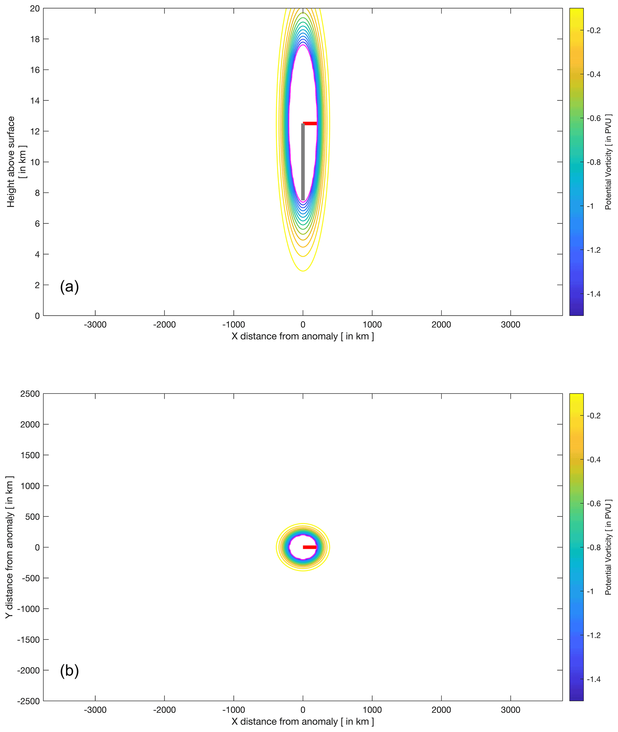
Figure 4 Example of a PV anomaly forced into the idealized domain by means of a longitudinal cross-section (a) and a horizontal cross-section (b) through the centre of the anomaly. The anomaly has a maximum horizontal width along the minor axis of 400 km and a height of 10 000 m. This excludes the “halo” of decreasing values to zero around it. The red line is defined as the anomaly radial width (x_size,y_size), whilst the grey line is defined as the anomaly radial height (z_size). The anomaly magnitude (in this case −1.5 PVU) is shown by the magenta contour.

The study examines how the meteorological fields changed based on a high-PV anomaly which is forced into the domain. It should be noted that this takes place in the southern hemispheric atmosphere where large negative values of PV are associated with cyclonic motion, contrary to the Northern Hemisphere where cyclonic motion is associated with large positive values. For the purposes of this study, high PV values are associated with large negative values of PV. The three-dimensional PV anomaly is given by

$$\begin{array}{}\text{(5)}& \begin{array}{rl}\mathrm{ANO}& =min\left\{-\mathrm{1.5},-\left(\mathrm{4}\times \left[e^{\frac{-(z-z_{\mathrm{pos}})}{z_{\mathrm{size}}}}\right]\times \left[e^{\frac{-(y-y_{\mathrm{pos}})}{y_{\mathrm{size}}}}\right]\right.\right.\\ & \left.\left.\times \left[e^{\frac{-(x-x_{\mathrm{pos}})}{x_{\mathrm{size}}}}\right]\right)\right\},\end{array}\end{array}$$

where x, y and z are its horizontal and vertical coordinates, x_pos, y_pos and z_pos are the x, y and z coordinates of the centre of the anomaly, and x_size, y_size and z_size are the horizontal and vertical radial dimensions. For this study, the anomaly magnitude is set at a standard value of −1.5 PVU. Equation (5) results in an anomaly with a minimum PV intensity of −1.5 PVU and which increases outward from the central minimum for a distance x_size, y_size and z_size. It is acknowledged that within real-world PV intrusions, there would likely be a decreasing PV gradient within the PV intrusion. However, within the experimental framework the interior of the PV intrusion is kept constant to more easily control the magnitude of the PV intrusion that results from the PV anomaly. An example of this anomaly is shown in the horizontal and vertical profiles in Fig. 4. The anomaly shown in Fig. 4 has x_size,y_size=200 km resulting in a total maximum width of 400 km. The specified z_size=5000 m results in a total vertical size of 10 000 km. This excludes a halo of increasing values around the specified anomaly. Applying an anomaly such as that shown in Fig. 4 results in a lowering of the values in the stratosphere. More importantly, the anomaly results in a tongue of high PV values emerging below the −1.5 PVU contour.

The control experiment (Experiment 0) is used as a reference. Experiment 0 uses the specified values above, namely a dynamical tropopause height of 12 500 m, an anomaly radial width of 200 km and an anomaly radial height of 5000 m. The meteorological changes that occur because of the introduction of the anomaly are then analysed, with special focus on surface cyclogenetic forcing as observed by the induced surface relative vorticity and surface pressure fields. Further, we test the effect of changes to four different parameters with respect to the anomaly and tropopause and their effect on cyclogenetic forcing at the surface. Surface cyclogenetic forcing is measured by means of changes in the induced relative vorticity and surface pressure for each intrusion scenario.

The first experiment (Experiment 1) systematically explores the effect of the depth of stratospheric intrusions on the induced cyclogenetic forcing at the surface. The effect that the depth of the stratospheric intrusion has on surface cyclogenetic forcing is tested by varying the anomaly radial height. Experiments are performed with anomaly radial height values lower (2500 m) and higher (7500 and 10 000 m) than the control experiment (Experiment 0, 5000 m). Experiment 1 is performed with a constant dynamical tropopause height of 12 500 m and a constant anomaly radial width of 200 km. The varied anomaly radial heights with a constant dynamical tropopause result in tongues of high-PV air extending further towards the surface, as observed in stratospheric intrusions and tropopause folds.

Secondly, the effect that the height of the dynamical tropopause above the surface has on surface cyclogenetic forcing is explored in Experiment 2. This experiment is comprised of three separate model experiments with varying dynamical tropopause heights with a constant anomaly radial height of 5000 m and a constant anomaly radial width of 200 km. Dynamical tropopause heights of 15 000 and 10 000 m are used and the results compared to the control experiment (Experiment 0, 12 500 m). This experiment gives us an indication of whether the depth of the stratospheric intrusion is more important than the proximity of the intrusion to the surface. This notion was hypothesized in Barnes et al. (2021a).

The third set of experiments, Experiment 3, reasserts the notion of stratospheric depth versus proximity to the ground. In Experiment 3, only the anomaly radial width is kept constant at 200 km. Both the dynamical tropopause height and the anomaly radial height are varied simultaneously such that the eventual height of the intrusion a.g.l. is similar. In this experiment we use dynamical tropopause heights of 15 000 and 10 000 m. Testing anomaly radial heights in 500 m intervals, we compare experiments that result in the closest stratospheric intrusion height a.g.l. compared to that of Experiment 0.

Experiment 4 considers the magnitude of the intruding anomaly and tests how it affects cyclogenetic forcing at the surface. For this experiment, the anomaly description remains the same as in Eq. (5). However, all values that are greater than the specified anomaly magnitude are assigned a value equivalent to the anomaly magnitude. A higher (−2 PVU) and lower scenario (−1 PVU) are tested and compared to the control experiment (Experiment 0, −1.5 PVU).

Table 1 Table of all experiments performed using the PV inversion algorithm. In each experiment, the basic state remains the same with varied dimensions of the PV anomaly, magnitude of the PV anomaly and the height of the dynamical tropopause a.g.l.

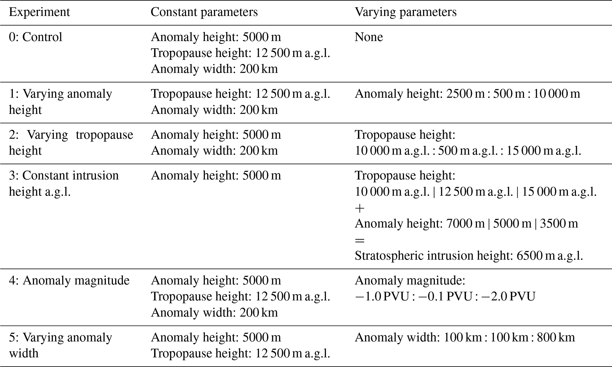
Finally, the effect that the horizontal size of stratospheric intrusions has on surface cyclogenetic forcing is tested by varying the anomaly radial width (Experiment 5). Tests with anomaly radial width values of 100, 200 and 400 km are performed with a constant dynamical tropopause height of 12 500 m and a constant anomaly radial height of 5000 m. All the above experiments are also provided in the flow chart shown in Table 1.

3 Results

3.1 Experiment 0: an idealized stratospheric intrusion and its effect on the domain

A basic, reference experiment is performed to reconstruct the conceptual model of a PV anomaly that extends from the stratosphere. Figure 5 shows a stratospheric intrusion simulated to a depth of 5000 m from the dynamical tropopause stipulated at 12 500 m a.g.l. The stratospheric intrusion has the standard horizontal radial width of 200 km. The −1.5 PVU contour is calculated to be at a height of 11 287 m a.g.l. (as described in Sect. 2.2). The stratospheric intrusion extends to a depth of 6594 m a.g.l. Figure 5 also shows the cyclonic motion that exists as a result of the stratospheric intrusion as is seen in the conceptual model in Fig. 1. The cyclonic motion is shown in Fig. 5 by the positive meridional wind velocities (wind flow “into the page”) shown by the solid grey contours to the west of the intrusion and the negative meridional wind velocities (wind flow “out of the page”) shown by the dashed grey contours. The resultant upper-level cyclonic motion emerges in the upper-level pressure fields as an amplified trough as shown in Fig. 6a. This re-emphasizes PV theory that shows that COLs are associated with high-PV intrusions of stratospheric air as shown by Hoskins et al. (1985). Although strong cyclonic rotation is confined to the area around the intrusion, weak cyclonic rotation is present throughout much of the cross-sectional domain, including the surface. This is shown by the outer-most wind velocity contours in Fig. 5.

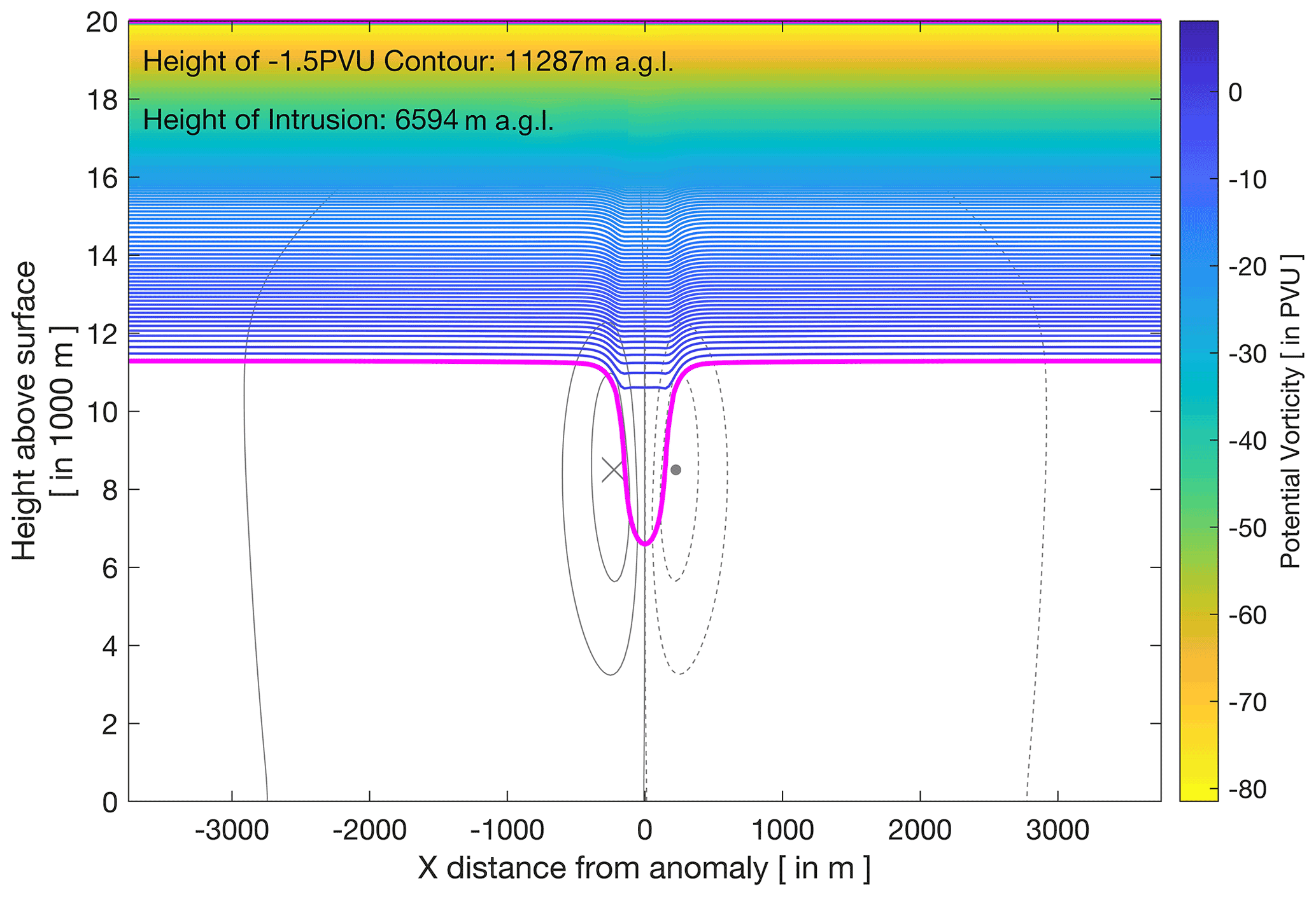
Figure 5 Stratospheric intrusion with a radial width of 200 km and depth of 5000 m from the dynamical tropopause specified at 12 500 m a.g.l. Meridional wind velocities are given in 4 m s⁻¹ intervals shown by the grey contours. Solid grey contours and the “X” indicate winds moving into the page, whilst dashed grey contours and the “dot” indicate winds coming out of the page.

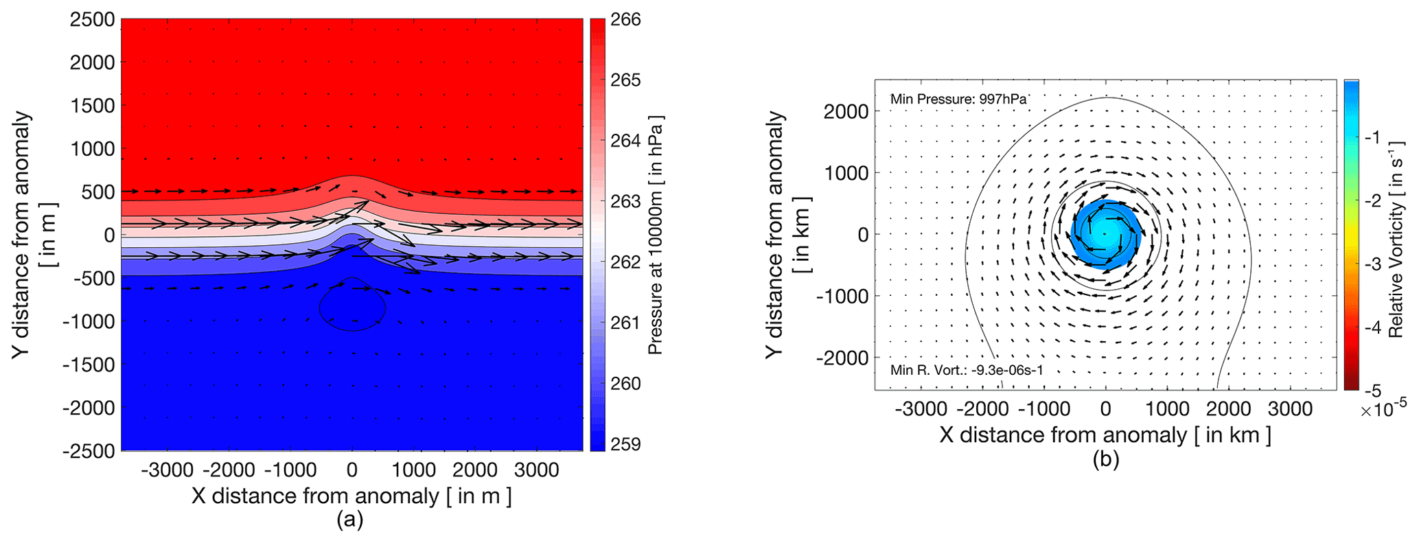
Figure 6 (a) Upper-level (10 000 m a.g.l., 2500 m below the experimentally defined dynamical tropopause) pressure field (shaded), together with wind vectors plotted as black arrows. (b) Surface pressure isobars (black lines) and surface relative vorticity (shaded), together with surface wind vectors plotted as black arrows.

Figure 6b shows the surface pressure isobars (black contours) together with the surface wind vectors. Before the introduction of the PV anomaly, this field is set at a constant 1000 hPa (see Sect. 2.2). It is clear that a surface pressure decrease and cyclonic rotation around the axis of the stratospheric intrusion is induced by the stratospheric intrusion, as predicted by theory. A drop of 3 hPa in surface pressure is observed after the introduction of the stratospheric intrusion. Relative vorticities within the centre of the surface circulation are shown by shaded colours in Fig. 6b. The lowest relative vorticity observed within the induced surface circulation is $-\mathrm{0.9}\times {\mathrm{10}}^{-\mathrm{5}}$ s⁻¹.

A similar intrusion was observed in the South Atlantic that resulted in a similar decrease in surface pressure and the development of a surface cyclone (Iwabe and Da Rocha, 2009). In that observational study, a similar pressure decrease was seen with the central surface pressure of the surface cyclone decreasing by 4 hPa within 6 h (Iwabe and Da Rocha, 2009; Table 1).

3.2 Experiment 1: varying stratospheric intrusion depth

The effect that the depth of the stratospheric intrusions has on surface cyclogenetic forcing is investigated by systematically varying the anomaly radial height (as defined in Sect. 2.2) of Experiment 0. The results of a selection of these varying stratospheric intrusion depth experiments are shown in Fig. 7, and a summary of the full set of experiments is shown in Fig. 8. Varying stratospheric intrusion depths are all compared to the control experiment as shown in Experiment 0. For ease of reference and comparison we show this experiment again in Fig. 7a2 and b2, and it is highlighted in green in Fig. 8.

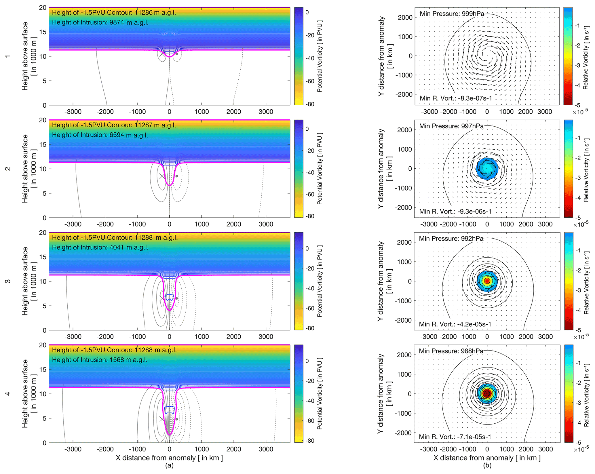
Figure 7 (a) Longitudinal PV cross-sections through the centre of the forced anomaly. The −1.5 PVU contour (our definition of the dynamical tropopause for this study) is highlighted by a thick magenta line. Meridional wind velocities are given in 4 m s⁻¹ intervals shown by grey contours. Positive velocities (into the page) are represented by solid contours, whilst negative velocities are represented by dashed contours (out of the page). (b) The effect of the intrusion on the surface pressure and relative vorticity are shown in the right panels. Pressure isobars at a 1 hPa contour interval are shown by black lines, whilst relative vorticity is shown by the shading. The panels in rows 1–4 represent different varying stratospheric depths introduced into the domain. For this experiment (Experiment 1), radial anomaly depths given to the system are 2500 m (row 1), 5000 m (row 2), 7500 m (row 3) and 10 000 m (row 4). By convention, in-text figure references refer to the column letter and the row number of the panel referenced (i.e. b2 refers to the panel in column b and row 2).

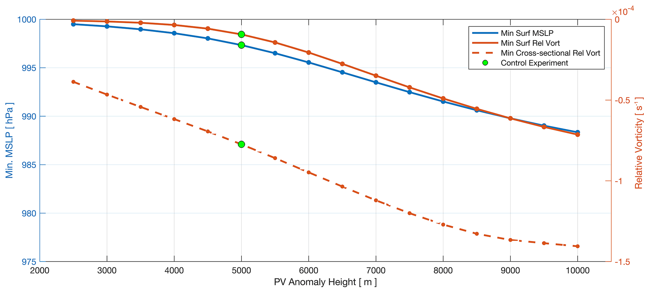
Figure 8 Changes to surface parameters (solid lines) as a function of anomaly radial height (depth of intrusion). The minimum mean sea level pressure (MSLP) (blue) and relative vorticity (orange) on the surface pressure level are recorded and plotted. The cross-sectional minimum relative vorticity as a function of anomaly depth is also shown by the dashed line. The results in Experiment 0 are highlighted in green for convenience.

A shallower intrusion depth compared to that in Experiment 0 resulted in weaker (lower velocity) cyclonic rotation around the stratospheric intrusion as shown in the shallow intrusion experiment in Fig. 7a1. Maximum meridional wind velocities are in fact almost half of that of Experiment 0 using half the anomaly depth (6 m s⁻¹ in Fig. 7a1 and b1 compared to 11 m s⁻¹ in Fig. 7a2 and b2). The area of the surrounding troposphere affected by even weak cyclonic flow is also smaller compared to that of the standard, deeper intrusion with a standard value of 5000 m (Experiment 0; Fig. 7a2 and b2).

In comparison, the converse is true for tropospheric intrusions which reached greater depths (as depicted in Fig. 7a3 and a4). Maximum meridional wind velocities of the deeper examples in Fig. 7 in fact strengthened to 17 m s⁻¹ (Fig. 7a3) and 22 m s⁻¹ (Fig. 7a4) using 7500 and 10 000 m anomaly depths respectively. The enhanced cyclogenetic forcing is also shown in Fig. 8 by the increase in the minimum cross-section relative vorticity (dashed lines). For the purposes of this work minimum cross-section relative vorticity is defined as the lowest value of relative vorticity in the longitudinal cross-section through the PV anomaly. Minimum cross-sectional relative vorticity increases almost linearly with a constant increase in PV anomaly depth but increases at a slower rate with anomaly depth greater than 8000 m. The growth in mid-level cyclogenetic forcing is stunted as the anomaly and mid-level jet core stretch closer to the surface. The location of the maximum mid-tropospheric meridional velocity (or mid-level jet core) is located closer to the surface for increased stratospheric intrusion depth.

Similar observations can be made when analysing the induced surface flow with changing stratospheric intrusion depth. As expected, shallower intrusions (less than the 5000 m used in Experiment 0) induce a weaker circulation occurring on the surface compared to Experiment 0 shown by increased relative vorticities for decreased intrusion depth. A smaller surface pressure anomaly is also induced with the smallest intrusion depth inducing a less than 1 hPa decrease in the surface pressure field (as seen in Fig. 7b1).

Increasing the depth of the high-PV anomaly conversely induces greater cyclogenetic forcing with a lowering in the central surface pressure anomaly and increased cyclonic rotation at the surface (Fig. 8). The centre of the induced surface pressure anomaly decreases sharply with increasing intrusion depth. The 7500 and 10 000 m anomaly radial heights (depicted in Fig. 7a3 and a4) induce an 8 and 12 hPa decrease (compared to 3 hPa in Experiment 0) in their associated surface pressures respectively. The observational study of Cape Storm in Barnes et al. (2021a) showed a decrease of 6 hPa on 7 June 2017 collocated with a stratospheric intrusion to the 550 hPa level. The intrusion, similar to that shown in Fig. 7a3, results in a similar response in the surface pressure. The enhanced cyclonic circulation is also depicted through the increasing relative vorticity present at the surface with increased PV anomaly depth.

The enhanced pressure decreases and cyclonic vorticity induced around deeper intrusions in this idealized framework echo the findings of Barnes et al. (2021a), who show that, in a climatological sense, deeper intrusions are associated with COLs that extend to the surface. It should however be noted that the study by Barnes et al. (2021a) includes a temporal aspect to the growth and development of surface cyclones induced by intrusions of different depths that this numerical experiment does not. Despite the lack of a temporal aspect, it is clear from within this experimental framework that surface cyclogenetic forcing and general tropospheric cyclonic motion are enhanced with intrusion depth. It also emphasizes the findings of Barnes et al. (2021a), which are that COL extension to the surface is a vertically coupled process, with cyclonic flow developing throughout the troposphere as the COL and surface low develop. This set of numerical experiments imply that deeper intrusions are more likely to induce enhanced cyclonic forcing in the surrounding troposphere and therefore result in a COLs extension to the surface.

3.3 Experiment 2: varying tropopause height with constant intrusion depth

The height of the tropopause is variable both spatially and seasonally (Kunz et al., 2011). In the austral summer months the meteorological Equator is situated south of the geographical Equator resulting in a raised tropopause, with the converse being true for the austral winter months. Additionally, the temperature differences between the Equator and the poles result in the dynamical tropopause being situated closer to the surface in the higher latitudes compared to the lower latitudes (Kunz et al., 2011). Barnes et al. (2021a) showed a distinct seasonality and latitudinal discrepancy in the number of COLs that extend to the surface, linking this variability to the height of the tropopause. Conditions with a lower tropopause (as found in winter and closer to the poles) tend to produce a greater number of COL extensions in the Southern Hemisphere than when the tropopause is further from the surface (in the summer months and closer to the Equator).

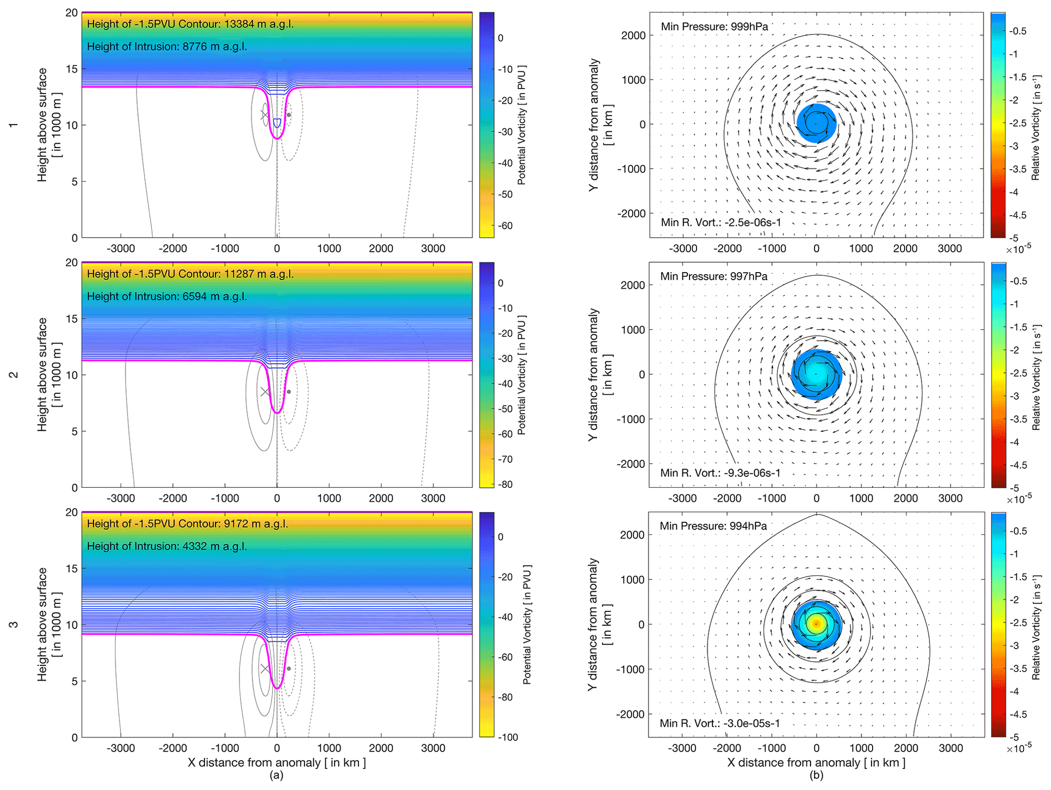
Figure 9 Same as in Fig. 7 with the exception that in this case the anomaly radial height is kept constant at 5000 m with varying tropopause heights of 15 000 m (row 1), 12 500 m (row 2), as in Experiment 0, and 10 000 m (row 3).

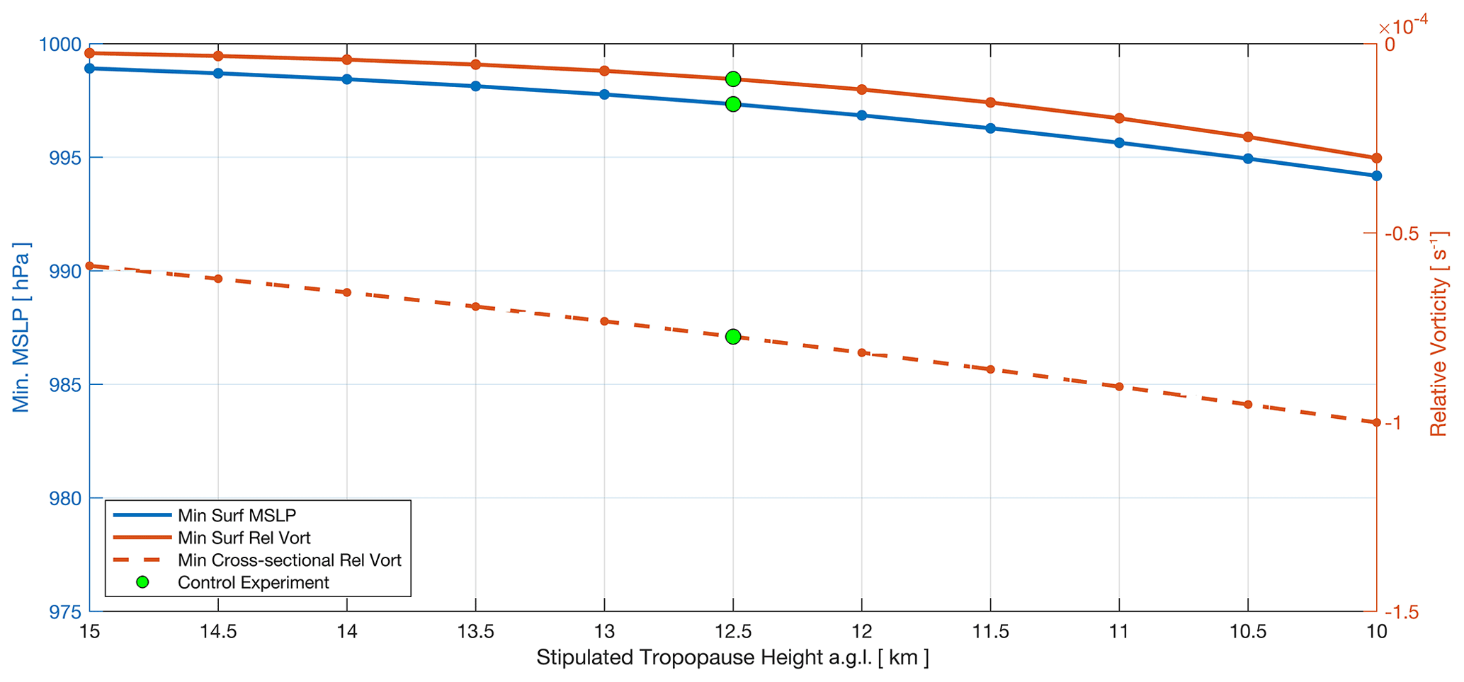
Figure 10 Similar to Fig. 8 but for Experiment 2 (varying tropopause height experiments) with tropopause height a.g.l. shown on the x axis.

The dependence of tropopause height on surface cyclogenetic forcing is explored here in a systematic and idealized way by changing the height of the specified tropopause with a constant anomaly radial height of 5000 m. The constant anomaly radial height simulates stratospheric intrusions of similar vertical extent (radial height) in different tropopause height regimes. The standard 12 500 m tropopause height a.g.l. (as seen in Experiment 0) is depicted by a higher scenario (tropopause height of 15 000 m) and a lower scenario (tropopause height of 10 000 m) in Fig. 9. A full set of experiments comprising various higher- and lower-tropopause scenarios and the induced cyclogenetic forcing are shown in Fig. 10. It should be noted that the tropopause height stipulated and the resulting −1.5 PVU contours (which denote our definition of the dynamical tropopause) do differ (see Sect. 2.2). The actual dynamical tropopause heights (−1.5 PVU contours) for the middle (Experiment 0), high (15 000 m tropopause) and low scenarios (10 000 m tropopause) are situated at 11 287, 13 384 and 9172 m a.g.l.

Figure 9a depicts the PV intrusions in the middle-, high- and low-tropopause scenarios. The decreasing height of the dynamical tropopause results in the stratospheric intrusions effectively being in closer proximity to the surface but with no change in the vertical extent (radial height) of the intrusion. The difference in tropopause height results in different heights of the associated stratospheric intrusion a.g.l. reaching 6594 m a.g.l. (Experiment 0), 8776 m a.g.l. (higher scenario) and 4332 m a.g.l. (lower scenario). The resulting effects on the surrounding troposphere and surface are shown in Figs. 9 and 10.

Similarly to Experiment 1, Fig. 9a shows the differences in the induced cyclonic circulation around the PV anomaly in the upper levels. The increasing dynamical tropopause height, even with a similar vertical PV intrusion extent (radial height), has a similar effect on the circulation around the anomaly as seen in Experiment 1. The enhanced mid-tropospheric circulation is readily seen in the decreasing minimum cross-sectional relative vorticities from the highest-tropopause to the lowest-tropopause scenarios (Fig. 10). Minimum cross-sectional relative vorticities show a decrease of about $\mathrm{4}\times {\mathrm{10}}^{-\mathrm{5}}$ s⁻¹ in the minimum cross-sectional relative vorticity between the high- and low-tropopause height scenarios. Maximum meridional velocities increase from 9 m s⁻¹ in the highest-tropopause scenario (Fig. 9a1) to 12 m s⁻¹ in the control (Experiment 0) and intermediate scenario (Fig. 9a2). The lowest-tropopause scenario (Fig. 9a3) contains a maximum meridional velocity of 15 m s⁻¹. The increased vorticity from one scenario to the next is not a function of the intensity of the anomaly since the amplitude of the anomaly is kept constant in Experiment 2. With no difference in the PV environment, it follows from Eq. (1) that

$$\begin{array}{}\text{(6)}& {\mathit{\zeta }}_{\mathrm{g}}+f=q-f{\displaystyle \frac{\partial }{\partial z}}\left({{\displaystyle \frac{\partial \stackrel{\mathrm{‾}}{\mathit{\theta }}}{\partial z}}}^{-\mathrm{1}}\mathit{\theta }\right).\end{array}$$

The environmental potential temperature gradient is set as constant since the tropospheric and stratospheric static stability values are kept constant throughout Experiment 2 (as explained in Sect. 2.2). Therefore, the term ${\frac{\partial \stackrel{\mathrm{‾}}{\mathit{\theta }}}{\partial z}}^{-\mathrm{1}}$ in Eq. (6) does not change between the high- and low-tropopause cases. As a result, the change in relative vorticity is controlled by a local change in the potential temperature gradient $\left(\frac{\partial \mathit{\theta }}{\partial z}\right)$. Calculation of this term within the intrusion shows that there is an increase in the local potential temperature gradient between three scenarios in Experiment 2. In fact, in the centre of the intrusion at the height of the maximum meridional velocity, the potential temperature gradient $\left(\frac{\partial \mathit{\theta }}{\partial z}\right)$ increases from 0.44 K m⁻¹ in the higher-tropopause scenario to 0.47 K m⁻¹ in lower-tropopause scenario. Since $\frac{\partial }{\partial z}\left({\frac{\partial \stackrel{\mathrm{‾}}{\mathit{\theta }}}{\partial z}}^{-\mathrm{1}}\right)<\mathrm{0}$ and both q and f are negative in the Southern Hemisphere, it follows that an increase in $\frac{\partial \mathit{\theta }}{\partial z}$ will result in a decrease in relative vorticity in the Southern Hemisphere. The more tightly packed potential temperature contours within the intrusion (higher static stability) in the scenario where the dynamical tropopause is closer to the surface result in a decreased cross-sectional relative vorticity compared to the higher-tropopause scenario.

Figure 10 shows that the induced cyclogenetic forcing increases at the surface with decreased tropopause height. This is seen by both the sharp decrease in pressure and relative vorticity at the surface. The intermediate scenario (Experiment 0) with an intrusion depth of 6594 m resulted in a 3 hPa drop in surface pressure. In contrast, with the same vertical intrusion depth, the intrusions from the higher dynamical tropopause (Fig. 9a1 and b1) induce only a 1 hPa decrease in the surface pressure. A stark contrast is seen in the scenario from the dynamical tropopause situated closer to the surface (Fig. 9a3 and b3​​​​​​​). The lower tropopause scenario resulted in a doubling of the pressure decrease at the surface (6 hPa) compared to Experiment 0 (3 hPa). Enhanced cyclonic circulation is induced at the surface in the lower-tropopause scenario as shown by an increase in the cyclonic surface relative vorticity.

The results of Experiment 2 clearly show that the effective height of the intrusion a.g.l. is a factor in the induced surface cyclogenetic forcing. With the same intrusion vertical depth, the experiments with lower intrusion height a.g.l. result in more intense lowering of the surface pressure. It should be noted that these tests were also repeated with different vertical depths of intrusion by using different anomaly radial heights of 2500 and 7500 m (not shown). The tests show a similar result in that intrusions associated with the higher tropopause result in a decreased cyclogenetic forcing than those associated with the lower tropopause.

3.4 Experiment 3: constant intrusion height from varying tropopause height and intrusion depth

The results in Experiments 1 and 2 imply that the proximity of a stratospheric intrusion to the surface has a larger impact on inducing deeper and enhanced cyclonic circulation at the surface than the vertical extent or size of the intrusion itself. This was also hypothesized by Barnes et al. (2021a) with respect to COL vertical extensions. In order to confirm this concept, anomalies are created such that they extend to a similar height a.g.l. from a varying tropopause height and are compared to Experiment 0 (Fig. 11a2 and b2). In this case anomalies with radial heights of 7000, 5000 and 3500 m were introduced into the fields with tropopause heights of 15 000, 12 500 and 10 000 m a.g.l. respectively. The resulting intrusions heights a.g.l. were calculated to be at 6750, 6594 and 6350 m a.g.l. respectively. All three of these intrusions induce cyclonic motion around the anomaly of similar vertical extent (radial height), with maximum meridional wind velocities between 11–12 m s⁻¹. The intrusions also all induce a similar surface level pressure deepening resulting in about a 3 hPa surface central pressure drop.

Figure 11 Same as in Fig. 7 but with variable anomaly radial heights such that the heights of the stratospheric intrusions a.g.l. are similar from varying tropopause heights of 15 000 m (row 1) and 10 000 m (row 3). Experiment 0 is given in row 2 for ease of reference.

Some small but noticeable differences can however be seen between the different scenarios in Experiment 3. The larger intrusion emanating from a higher dynamical tropopause (Fig. 11a1) results in a slightly deeper penetration of the high-velocity core around the simulated anomaly compared to anomalies with less vertical extent (radial height) in Fig. 11a2 and a3. In Fig. 11a1 the 4 m s⁻¹ contour extends to a depth 1000 m deeper than in Fig. 11a2 and a3. The effect of this is also noticeable on the surface. Relative vorticities on the surface increase slightly with intrusion vertical extent (radial height) with a decrease of $\mathrm{3}\times {\mathrm{10}}^{-\mathrm{6}}$ s⁻¹ from the lowest-tropopause (small anomaly vertical extent) scenario in Fig. 11a3 to the highest-tropopause scenario (large anomaly vertical extent) in Fig. 11a1. A major difference between these scenarios is the presence of a −2 PVU anomaly within the intrusion in Fig. 11a1 that does not appear in Fig. 11a2 or a3. This is an artefact of the basic state setup but could be influencing and enhancing the additional rotation at the surface. The influence of anomaly magnitude will be further investigated in Experiment 4.

3.5 Experiment 4: varying anomaly magnitude

Experiment 3 brings forth the question of the magnitude of the stratospheric intrusion with respect to its effect on the cyclonic circulation at all tropospheric levels around the anomaly. Experiment 4 tests this effect by changing the magnitude of the intrusion, i.e. by varying the anomaly amplitude. A lower (−1.0 PVU) and higher (−2.0 PVU) scenario are tested and shown in Fig. 12. For ease of reference, the −1.0 PVU contour is also plotted as a dashed magenta line in Fig. 12. As our definition of the tropopause continues to be −1.5 PVU, the resulting intrusion of the lower scenario is very shallow but does contain a small anomaly close to the depth of Experiment 0 (Fig. 12a2). Figure 13 shows that the magnitude of the intrusion has some effect on the mid-tropospheric cyclogenetic forcing. Minimum cross-sectional relative vorticity decreases by $\mathrm{3}\times {\mathrm{10}}^{-\mathrm{5}}$ s⁻¹ from the low to high anomaly amplitude scenarios, whilst the maximum meridional velocity decreases by 1 m s⁻¹ around the anomaly. Anomalies of all magnitudes tested induce similar cyclogenetic forcing upon the surface. Both the induced surface pressure and relative vorticity are comparable throughout the scenarios tested.

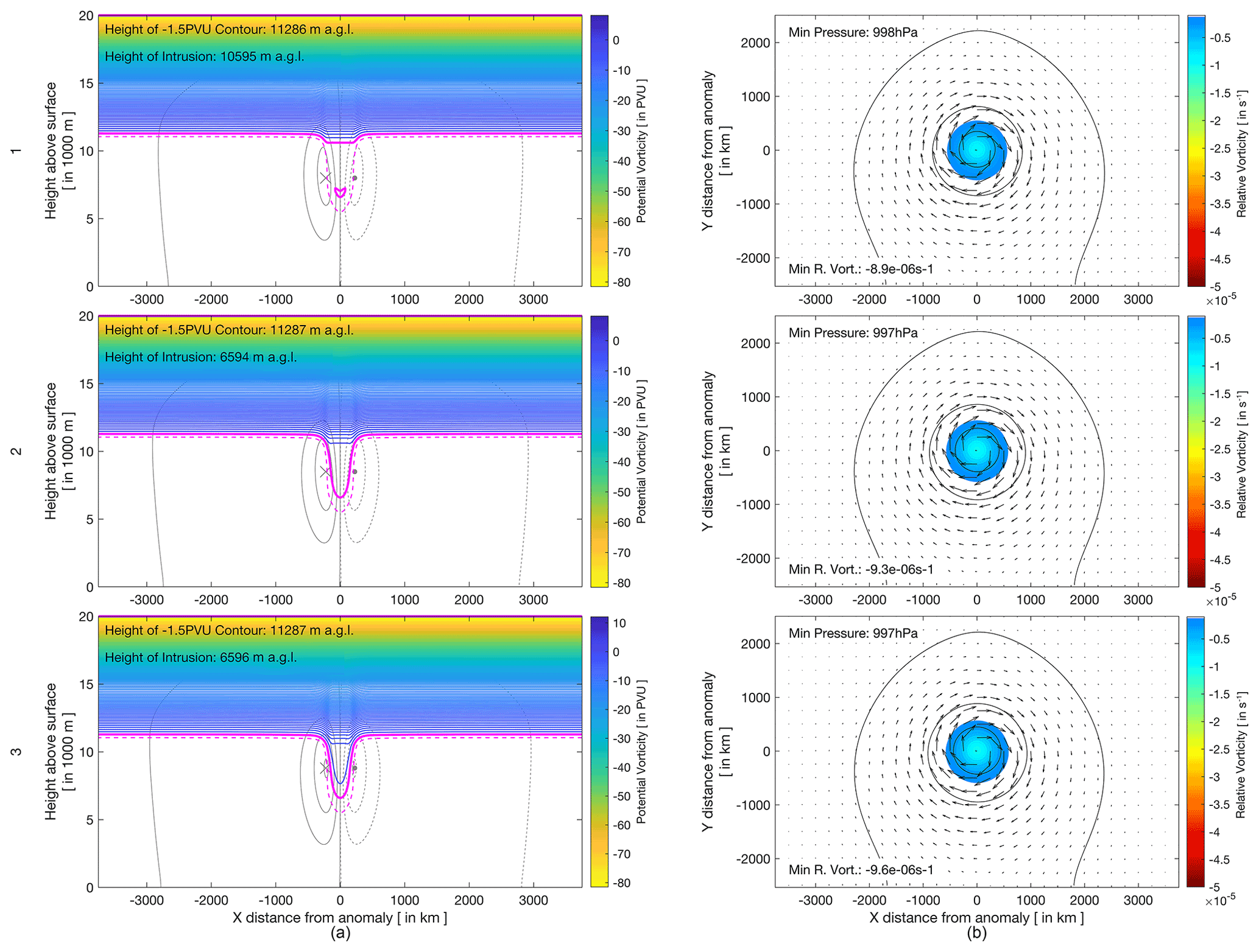
Figure 12 Same as in Experiment 0 with varying anomaly magnitudes of −1.0 PVU (row 1) and −2.0 PVU (row 3). Experiment 0 (with an anomaly magnitude of −1.5 PVU) is shown in row 2. In addition to the −1.5 PVU contour (thick magenta line), the −1.0 PVU contour is also provided for context by a dashed magenta line.

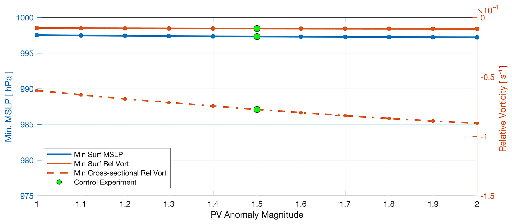
Figure 13 Same as in Fig. 8 but for Experiment 4 (varying stratospheric intrusion magnitude experiments).

The intrusions created as a result of this experimental setup are relatively flat anomalies with no gradient within the anomaly itself. As such the PV gradient structure between the different magnitude anomalies will be relatively similar between each of the scenarios and therefore will have little effect on the induced cyclonic circulation around the anomaly. In the real-world atmosphere, the anomaly is likely to have more of a gradient within the intrusions with a specified contour boundary. However, it is unlikely the maximum PV value within an intrusion would be an extreme PV value that is far greater than the PV value of the dynamical tropopause (see examples in Sprenger, 2007; Barnes et al., 2021b). The result therefore implies that it is less crucial which dynamical tropopause PV value an intrusion is analysed with than the geometric characteristics of the PV contour itself. The results of Experiment 4 reaffirm the findings in Experiment 3, i.e. that the vertical extent of the stratospheric intrusion could play a more vital role in affecting surface circulation than the magnitude of the PV intrusion.

3.6 Experiment 5: varying anomaly horizontal width

RWB events, which are associated with isentropic transport of stratospheric air into the troposphere, have been classified into four distinct categories, namely cyclonic equatorward breaking (LC2), cyclonic poleward breaking (P1), anticyclonic equatorward breaking (LC1) and anticyclonic poleward breaking (P2) (Thorncroft et al., 1993; Peters and Waugh, 1996). These different types of RWB events are associated with differing characteristics of the isentropic PV filaments produced and therefore differences in the geometric characteristics of the PV intrusions and the weather patterns they produce. Elongated, thin filaments of stratospheric air are produced by LC1-type breaking events because of the anticyclonic shear on the equatorward side of the PV structure (Thorncroft et al., 1993). These associated PV filaments eventually roll up and often produce cut-off PV structures. P1 events are also associated with thinner filaments of high-PV air (Peters and Waugh, 1996). Similarly to P2 events, LC2 events are associated with broader high-PV streamers which, under the influence of cyclonic shear, wrap cyclonically and do not result in cut-offs (Thorncroft et al., 1993). Recent examples of the different breadths of these streamers can be seen in Barnes et al. (2021b), where a thin PV streamer (of ∼ 1^∘ ≈ 100 km) and broader streamer (of ∼ 10^∘ ≈ 800 km) affected and deepened a surface cyclone.

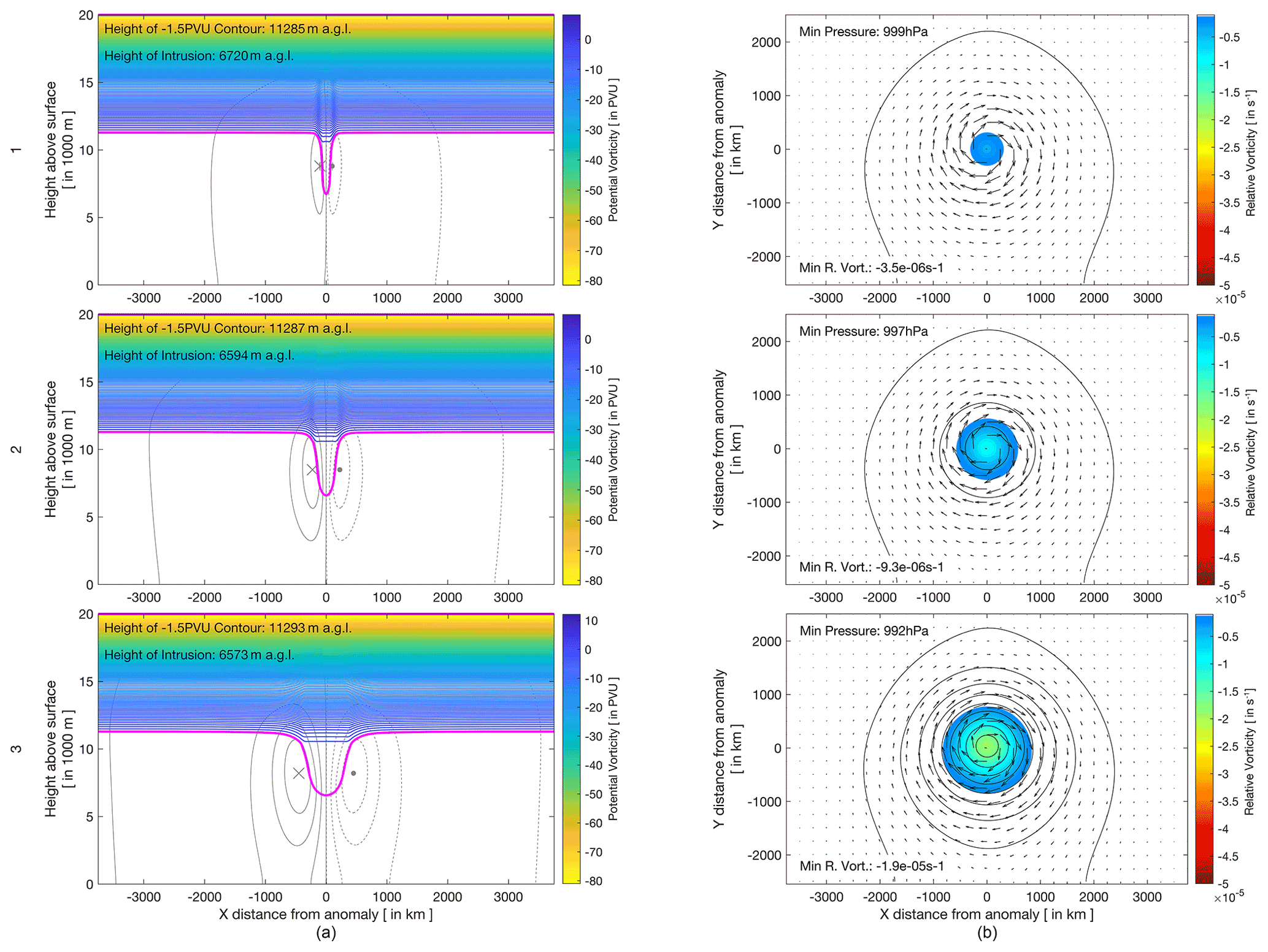
Figure 14 Same as in Fig. 7 but with variable anomaly radial widths such that the heights of the stratospheric intrusions a.g.l. are similar from a constant dynamical tropopause depth of 12 500 m. The thinner intrusion is created by an anomaly with a 100 km radial width (row 1), whilst the broader intrusion is created by a 400 km radial width (row 3). Experiment 0 (200 km radial width) is provided in row 2 for convenience and comparison.

Figure 15 Same as in Fig. 8 but for Experiment 5 (varying anomaly radial width experiments).

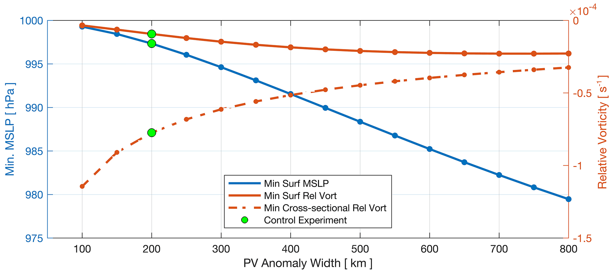
The effect that the width of the intrusion has on surface cyclogenesis is tested with a numerical setup similar to that of Fig. 4 with varying anomaly radial widths. Selected width experiments are shown in Fig. 14, and a summary of the effect of all experiments effect on surface parameters is shown in Fig. 15. All stratospheric intrusions were defined such that they reach a similar depth (using a constant 5000 m anomaly radial height from the 12 500 m a.g.l. dynamical tropopause).

Clear differences in the circulation around the anomaly can be seen in Figs. 14a and 15. The thinner intrusion (100 km width) in Fig. 14a1 results in a decrease in the maximum mid-tropospheric meridional velocities compared to the standard configuration (8 m s⁻¹ compared to 11 m s⁻¹ in Experiment 0). Conversely, the wider intrusion results in an increase in the maximum mid-tropospheric meridional velocities compared to the standard configuration (15 m s⁻¹ compared to 11 m s⁻¹ in Experiment 0). The corresponding cyclonic circulation is augmented by the breadth of the intrusion. The change in intrusion width results in a change in the geometry of the resultant jet core which appears thinner and shorter for the thinner anomaly. In contrast, the broader anomaly results in a visibly broader and longer jet core, affecting almost the entire cross-sectional domain. Although stronger velocities are observed in the troposphere as a result of broader intrusions, the mid-tropospheric relative vorticity increases sharply for broader intrusions (Fig. 15). The larger-magnitude mid-tropospheric relative vorticities induced by thinner intrusions are the result of the enhanced circulation in the mid-troposphere being confined to a smaller horizontal region around the anomaly.

The width of the intrusion is also important for surface parameters. The thinner intrusion results in a reduction in the cyclonic rotation as shown by the induced surface relative vorticity in both Figs. 14 and 15. The surface pressure field additionally responds to the width of the intrusion. The thinner PV intrusion results in a shallower surface pressure anomaly with a surface anomaly of 1 hPa induced by the thinner intrusion (compared to 3 hPa in the control experiment). Conversely, the broader intrusion induces a deeper surface pressure anomaly (to 8 from 3 hPa). Figure 15 shows that the surface pressure minimum decreases quasi-linearly with linear increasing PV anomaly width. In contrast to the mid-tropospheric relative vorticity, enhanced surface cyclonic rotation is induced by the broader PV anomaly as shown by with decreases in the surface relative vorticity. Decreases in the relative vorticity on the surface are however much less significant compared to the deepening experiments conducted in Experiments 1 and 2. Only a slight decrease in the minimum relative vorticity on the surface is discernible between the thin and broad scenarios (Fig. 15). The broader anomaly results in a wider (horizontal) distribution of surface pressures. An enhanced surface pressure gradient is therefore necessarily induced by increasing the radial width of the PV anomaly, resulting in a similar degree of cyclonic vorticity at the surface.

4 Discussion and conclusion

The study by Barnes et al. (2021a) showed a climatological link between COL depth and stratospheric intrusion depth. Deep COLs, those associated with surface cyclones, were generally found to be associated with deeper stratospheric intrusions. The reanalysis-based climatology of Barnes et al. (2021a) is performed in the context of the real-world atmosphere, where a host of processes at various levels of the atmosphere can affect the development of cyclones at all levels. Therefore, it is pertinent to isolate the link between the depth of their associated upper-level high-PV anomalies with the induced surface cyclogenetic forcing in an idealized setting. An initial numerical experiment using PV inversion diagnostics (Experiment 0) shows that the numerical model and PV inversion algorithms produce results as we expect from the conceptual model (Fig. 1) of a high-PV anomaly in the upper levels: a core of cyclonic flow is present around the PV anomaly, with general cyclonic motion prevalent, although weak, through the majority of the domain. The longitudinal cross-section and upper-level pressure and wind field show that the high-PV anomaly results in a trough, as is expected by theory. In the real-world atmosphere, the trough with continual amplification could develop into a COL. Cyclonic flow and low-pressure signatures are also observed on the surface. This re-emphasizes that upper-level processes induce both the surface cyclone and its associated COL. For Experiment 0, cyclogenetic forcing is very weak or negligible, although relative vorticities indicate that we are on the precipice of surface cyclogenetic forcing being induced. The anomaly does however induce a closed low pressure on the surface.

Experiment 1 varies the depth of a stratospheric intrusion (i.e. the closest distance of a −1.5 PVU point to the surface). This experiment reveals that the depth that a stratospheric intrusion reaches is an important factor in the induced surface cyclogenetic forcing. Very shallow intrusions result in a minimal pressure decrease on the surface, whilst extremely deep intrusions resulted in a pronounced decrease in surface pressure. Cyclonic circulation as measured by meridional velocities and relative vorticities is enhanced by deeper intrusions. This confirms the findings of Barnes et al. (2021a) that COLs associated with deeper high-PV intrusions are more likely to extend towards the surface. Barnes et al. (2021a) showed that COLs are more likely to be associated with a surface low if a stratospheric intrusion reaches below the 300 hPa level. Using a simple barometric conversion from altitude to pressure with standard sea level pressure and temperature reveals that the stratospheric intrusions shown in Experiment 1 (Fig. 7) extend to roughly the 270, 430, 610 and 840 hPa levels. This corresponds well with the findings of Barnes et al. (2021a) with the only intrusion extending to less than 300 hPa, inducing little cyclogenetic forcing on the surface.

Barnes et al. (2021a) showed that shallow COLs, COLs which only extend into the mid-levels, occur most frequently in the summer months and the lower latitudes. This corresponds to seasons and regions where the dynamical tropopause is furthest away from the surface. This finding, together with the finding that shallow COLs are most often associated with shallow intrusions, suggested that the height a.g.l. of the stratospheric intrusion is more important than the vertical depth of the intrusion itself. Experiments 2 and 3 show that this is indeed the case. Intrusions from high tropopause heights, as would be seen closer to the tropics and in summer, resulted in negligible cyclogenetic forcing at the surface and initiated very little pressure decrease at the surface (Experiment 2). Conversely, lower dynamical tropopauses induce enhanced surface cyclogenetic forcing and a large surface pressure decrease. Differing intrusion depths to a similar intrusion height a.g.l. were also shown to result in similar pressure deepening (Experiment 3). It was however shown the cyclonic motion at the surface was more enhanced, however slight, for the larger vertical intrusions compared to the smaller vertical intrusion. The enhanced relative vorticity in the large intrusion suggests that the vertical height of intrusion could play a role in the extreme windstorms (e.g. Liberato, 2014). Of course, it should also be noted that anomalies at the surface and in the low levels can also enhance cyclogenetic forcing when in phase, as shown in the example of Cape Storm by Barnes et al. (2021a).

The relative contribution of different factors to surface cyclogenetic forcing is highlighted in this study. Experiments 1–3 show that it is the depth that the stratospheric intrusion reaches that is the major factor in surface cyclogenetic forcing. Larger intrusions induce greater cyclogenetic forcing in the mid-levels than smaller intrusions. However, if the PV intrusions are situated further away from the surface (from a tropopause further away from the surface), the resulting relative vorticity on the surface is diminished and is comparable to that of a smaller intrusion extending to a similar height a.g.l. from a tropopause height closer to the surface. In terms of surface relative vorticity, wider intrusions are found to have a small but largely negligible effect despite the dramatic effect that these differences have in the mid-troposphere. The widths of these intrusions do still have a large effect on the surface pressure beneath them. With constant stratospheric depth (5000 m) and constant tropopause height a.g.l. (12 500 m), a thin filament intrusion with a radius of 100 km resulted in a minimal pressure decrease at the surface. Interestingly, the degree of surface pressure was comparable to that of the intrusion of double the width (200 km) and half the vertical extent (2500 m) as seen in Experiment 1 (Fig. 7, top panels).

Conversely, an intrusion with a large area and with a radius of 400 km resulted in a slightly deeper surface low pressure comparable to that of the intrusion with half the width and 50 % more depth as shown in Experiment 1 (Fig. 7, bottom panels). The resulting surface pressure and relative vorticity patterns together provide a picture of the weather systems being forced on the surface. Wider intrusions produce wider, deeper cyclonic circulations, whilst thinner filaments of PV produce shallower, smaller cyclonic circulations.

Conceptually, there is a distinct difference between the surface cyclonic circulations induced by the idealized intrusions presented here and which occur in reality. This is explained fully in Hoskins et al. (1985) and was touched on in Barnes et al. (2021a). Surface lows are generally found to the east of the COL and upper-level PV anomaly axis. In these idealized cases, however, the centre of the induced surface cyclonic motion is directly beneath the PV anomaly. In the real atmosphere, the surface cyclonic motion induced by the upper-level anomaly acts as a mechanism for warm surface temperature advection to the east of the upper-level anomaly. This surface temperature (and therefore potential temperature) anomaly has PV-like properties and can induce its own surface cyclonic circulation. Deeper intrusions will therefore drive more intense warm-air advection to the east of the trough axis, inducing enhanced cyclogenesis. One of the major limitations of this work is the lack of a temporal aspect in the experimental framework. Surface cyclones are not produced instantaneously but grow over time. Additionally, in the real-world atmosphere, upper-level PV anomalies are also influenced by the vertical structure of the air column and thermodynamic properties of the air beneath it. Future work should include the use of a numerical dynamical core which will have a temporal element and include processes such as upper-level induced surface warm-air temperature advection in a more realistic baroclinic environment. This would also improve the general analysis of the temporal aspect of intrusions as they grow and decay and the resulting effect on surface cyclogenesis. A dynamical core would also allow for the study of more complex vertical structures such as the inclusion of temperature inversions beneath the PV inversion.